Life-cycle expenditure allocations and the consumption costs of …uctp39a/BanksBlundellPrestonEEA... · 2011-03-20 · European Economic Review 38 (199-t) 1391-1410. North-Holland

European Economic Review 38 (199-t) 1391-1410. North-Holland

Life-cycle expenditure allocations and the consumption costs of children*

James Banks

Institute for Fiscal Studies, London, UK

Richard Blundell

Institute for Fiscal Studies, London, UK and University College London, London, UK

Ian Preston

Institute for Fiscal Studies, London, UK and University College London, London, UK

Received October 1991, final version received March 1993

In this paper we assess whether it is changing needs or intertemporal substitution that dominate household expenditure responses to the presence of children over the life-cycle. We construct lifetime expenditure paths for households with different demographic proliles and consider the shape of these paths and some possible implications for welfare measures. Simulated expenditure paths based on consistent single-period and multi-period models indicate that it is indeed changing needs that dominate such paths in periods when children are present in the household. However, allowing for intertemporal substitution is still shown to be important since it can introduce new information relevant to the calculation of household welfare.

1. Introduction

Attempts to estimate the ‘costs of children’ from household responses to differences in demographic type have concentrated attention largely upon observing differences in the composition of spending in a single period. The

Correspondence to: James Banks, Institute for Fiscal Studies, 7 Ridgmount Street, London WCIE 2AE, U.K.

*An earlier version of this paper was presented at the IFS conference on the Measurement of Household Welfare. This research was supported by funding from the Rowntree Foundation and from the Economic and Social Research Council. Research on the paper by Ian Preston was mainly carried out while working at Nuffteld College, Oxford. We are grateful to the Department of Employment for providing the Family Expenditure Survey. Paul Johnson provided extensive asistance with the creation of our dataset. and the paper has benefited from the useful comments of Guglielmo Weber, Arthur Lewbel and three anonymous referees. We alone, however, are responsible ‘for any errors.

0014-2921/94/%07.00 0 1994 Elsevier Science B.V. All rights reserved

SSDI 0014-2921(93)EOO51-L

1392 J. Banks et al.. Lfe-qcle expenditure and costs of children

question we ask here is to what extent the presence of children coincides with a reallocation of life cycle expenditure, and not simply a reallocation of ‘within-period’ expenditure shares. To the extent that life-cycle reallocations are made, we argue that standard measures of the consumption costs of children can be severely misleading.

It would seem natural to expect household expenditure paths and consumption growth to be influenced by anticipated demographic change, and the results of this paper suggest that this is indeed the case. Households clearly save in anticipation of times when children are present and, given this behaviour, expenditure in all periods of the life-cycle will depend upon the complete demographic profile of the household in all time periods. One of the main issues raised in this paper will be whether it is changing needs or intertemporal substitution that dominate the response of life-cycle expenditure profiles to demographic change. If children make consumption more expensive, then they would tend to lead to substitution away from child- rearing periods. However, increases in needs in periods when children are present will tend to counteract (and, we find, dominate) this effect. We estimate consistent life-cycle expenditure and single-period expenditure-share models that allow us to simulate life-cycle expenditure profiles for households with differing demographic futures. To the extent that we can associate welfare levels with these expenditure paths, one can also use them in an analysis of the costs of children.

The costs of children can be seen as the additional expenditure needed by a household with children to restore its standard of living to what it would have been without them. To implement this one might think of comparing the expenditures of two households, one with and one without children, yet sharing a common level of welfare. The difficulty in this is in finding a criterion which might allow one to identify when two households of different composition are at a common living standard. While economic analysis of demand behaviour can provide important information on the way household expenditure patterns change in response to demographic change, it cannot identify preferences over composition itself and cannot identify costs of children without making assumptions about these preferences [see Pollak and Wales (1979), Blackorby and Donaldson (1991a, b), Blundeil and Lewbel (1991), for example]. The placing of consumption costs in an intertemporal context highlights the problem of identifying the costs of children from observed demand behaviour by providing information on costs that are not recoverable from standard demand analysis.

The technique that we choose is sequential. We first estimate a standard demand system that is quadratic in the logarithm of total expenditure using a large sample of U.K. households for the period 1970-1988. We then use parameters from this system in estimating a model of intertemporal expenditure allocations using a time series of cohort-level data from the same

J. Banks et al.. Lift-cycle expendirurr and costs oj children 1393

sample. Together, these two stages of estimation provide all the parameters necessary to identify household expenditure decisions over time.

The layout of the paper is as follows. In the next section we consider the theoretical specification of a life-cycle framework for expenditure allocations that is consistent with a model of single-period spending, and section 3 discusses the implications of such a framework for the calculation and measurement of equivalence scales. Section 4 describes our usage of the pooled cross-sections of the U.K. Family Expenditure Survey to recover within-period and intertemporal preferences for households of different composition. In section 5 we outline our simulation methodology and present some simple simulation results. Section 6 concludes.

2. Model specification

2.1. Expenditure allocations and household composition

Suppose household preferences can be characterised as satisfying intertemporal additive separability. That is to say that the household’s preferences can be represented by a function U =C; u,(qt,z,) where qt represents the vector of consumption goods, I, a vector of household characteristics in period t and the function u,(.) incorporates the household’s subjective discount rate. We assume that consumers choose their most preferred allocation of expenditures over time subject to the constraint that the discounted value of life-time expenditures equals the present value of life-time wealth. The additive separability assumption over time allows us to separate the optimisation problem into two stages. Total consumption is first allocated between time-periods, and then, subject to this upper stage allocation, each period’s consumption is distributed between commodity groups [Gorman (1959)].

Under such assumptions, within-period preferences may then be represented by a function u,(x,,~,,t,) where x, is the (discounted) total expenditure allocation to period t and pt is the vector of discounted commodity prices. Moreover, intertemporal utility is given by

where F, now incorporates the subjective discount rate. As Blundell et al. (1989) show, within-period behaviour can only identify the indirect utilities u,(.) while intertemporal expenditure allocation may allow us to recover F,(.).

Optimisation, subject to perfect capital markets, leads to a chosen consumption path along which the marginal utility of within period (discounted) expenditure, i.,r i3F,/ax,, remains constant [see, for instance, Browning et al. (1985)]. The implied equation describing the dynamics of

1394 J. Banks et al., Life-cycle expenditure and costs of children

- 3.5 4.0 4.5 5.0 5.5 6.0

LOGX

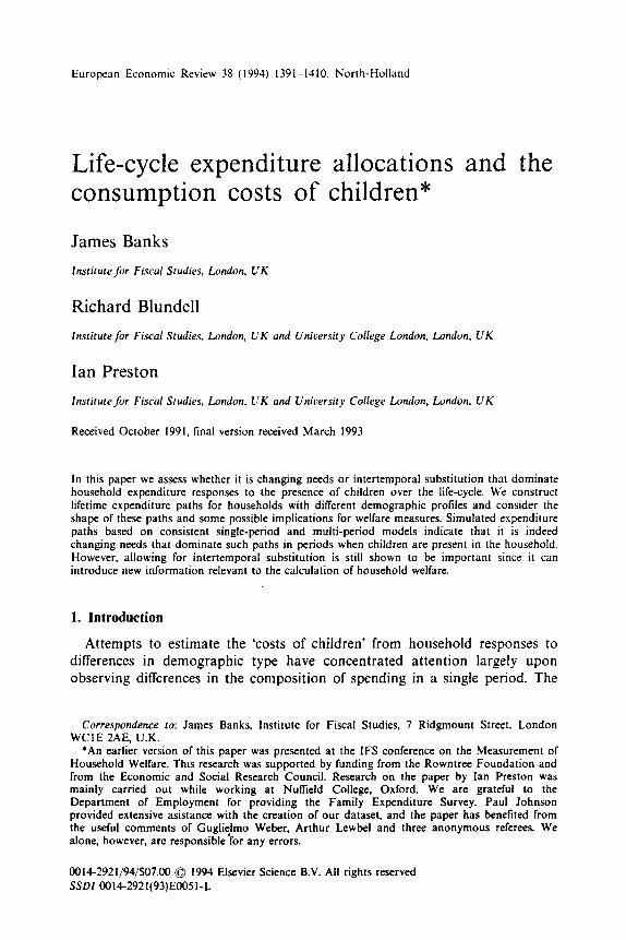
Fig. 1. Non-parametric Engel curve for ‘necessities’ (food, fuel and clothing).

consumption provides a means, given suitable data, of estimating the information necessary to identify F,(.). With uncertainty,’ about future real incomes for instance, R, evolves according to the familiar stochastic Euler equation [see Hall (1978) or MaCurdy (1983) for example]:

E,_,i.,=1,_,~-AlnI,~&,, (2.2)

where E, has a positive expectation’

2.2. Within-period expenditures

The empirical specification we adopt below involves a choice of functional form for within-period indirect utility which reflects the need for quadratic Engel curves in line with the growing body of empirical evidence. Fig. 1 illustrates the need for nonlinearity by showing a kernel regression of the share of expenditure spent on ‘necessities’ (i.e. food, fuel and clothing) on the logarithm of deflated total household expenditure within one demographi-

‘What has been said above has ignored uncertainty for simplicity of exposition, but nothing in our estimation methods is undermined if we allow for it.

‘If E, is normally distributed this expectation is equal to half its variance conditional on the given information [see Blundell et al. (1989)]. For a simple proof apply Jensen’s inequality to (2.2) and write -E,_,s,=E,-,(ln[I,/I.,_,])cIn[E,_,(I,/I,_,)]=O.

J. Bunks er ~1.. Lij+cycle expenditurr and costs of children 1395

tally homogeneous population. 3 The appropriateness of a quadratic speciti- cation is more fully argued in Banks et al. (1992) where the underlying indirect utility function is also derived.

In particular the indirect utility function underlying quadratic Engel curves takes the form

u,(.GP,, z,) = [b,lln c, + #+I - ‘, where c, = x,/a@,, z,), (2.3)

where c, is real expenditure, a, = a(~,, t,) is a linear homogeneous price index. and 6, = b(p,, I,) and 4,= (Pbr, z,) are zero homogeneous in prices.” The demographics in the a,, b, and 4, functions reflect the possibility that demographic variables may shift within-period preferences. Such a specitica- tion reduces to the convenient Almost Ideal type form [see Deaton and Muellbauer (1980)] if 4, is omitted, but otherwise leads to within-period budget shares w, that are quadratic in the log of total expenditure,’ and given by

C?lnp, ahip, ’ dlnp, b, ’

= xi(PI; t,) + pi@,; Z,) In C, + l+!li(Pr, tl) In C:. (2.4)

The specification in (2.4), however, remains flexible enough to sustain linear Engel curves for some goods (if t+Qi=O) and also allow demographic variables z, to alter the shape of these Engel curves.

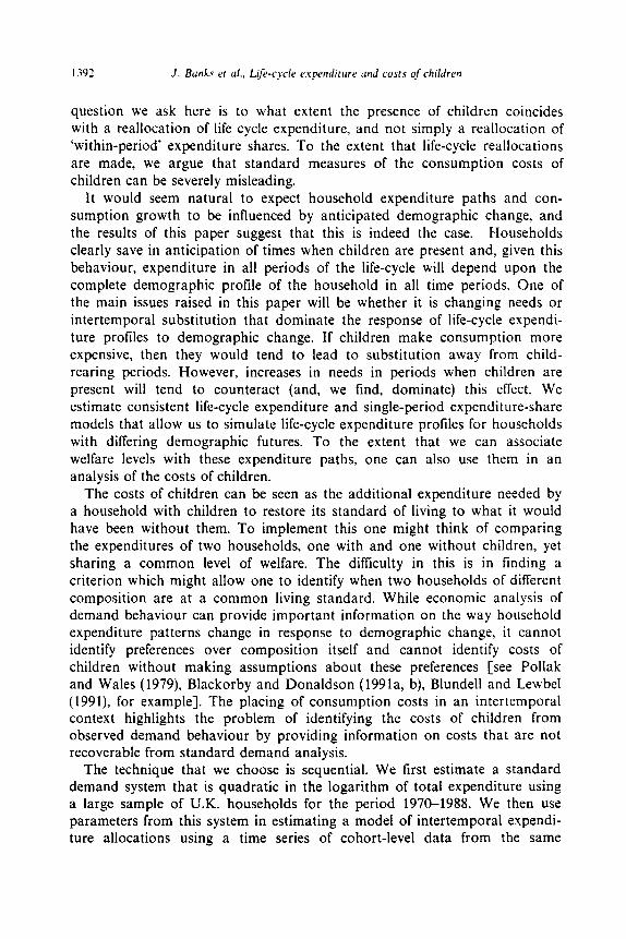
The need for such elements is graphically illustrated in fig. 2 where we present non-parametric Engel curves for food using the same data as fig. 1. We show kernel regressions that are split by the number of children in the household and there is clear need to allow the presence of children to shift at least the intercept of any Engel curve. Incidentally, the near-linearity of the food Engel curves indicated here (and the relative size of the food budget share) also implies that the underlying curvature in fuel and clothing expenditures must be strong to generate a kernel regression such as that in fig. 1.

2.3. Intertemporal expenditure allocations

Intertemporal preferences are specified by the following parameterisation of (2.1):

‘The data for this figure is a sub-sample of married couples without children from the Family Expenditure Survey data described in section 4.1 below. In addition we have simply chosen three years of data (1980-1982) to abstract from issues of comparability of prices and incomes across time. The points marked with crosses show pointwise contidence intervals evaluated at the nine decile points of log expenditure.

4Note that since b,, 4, and c, are zero homogeneous it is only when working with II, that we need to be careful with discounting considerations.

sThis is, in fact, shown by Lewbel (1988) to be the only integrable rank three demand system with budget shares linear in a constant, log expenditure and any other function of expenditure.

J. Banks et al.. L&r-cycle rxpenditurr and costs qf childrrn 1396

t 0 1 2 3 Split by TOT-KIDS

. 6

OL,,,,,,,,,,,,,,,,,,,,,,,,,

' 3.6 3.8 4.0 4.2 4.4 4.6, 4.a 5.0 5.2 5.4 5.6 5.8 6.0

LN_EXP Fig. 2. Non-parametric Engel curves for food split by number of children.

Here, information in 6, = 6(z,) and pt = p(z,) is important and identifiable only within an intertemporal framework.6 The parameters of both are concerned with intertemporal preferences, as explored (with a different within-period specification) by Blundell et al. (1993). The presence of a term like 6, is attractive because we wish to allow for the possibility that the presence of children in certain periods may make spending in those periods more or less appealing independently of the impact of children on the within-period composition of spending. Such an effect cannot be picked up by traditional single-period analyses.

The term pt is included to allow us to estimate the degree to which parents are prepared to substitute expenditure away from the relatively expensive periods when children are in the household. The within- and cross-period parameters jointly establish the concavity of F,(e) and hence the intertemporal elasticity of substitution, c,, defined as the reciprocal of the elasticity of marginal utility with respect to period t expenditure [see Browning (1987, 1989)]:

6We have omitted any component to F,(.,z,) that cannot be identified from expenditure data alone.

J. Bunks et al.. Lije-cycle e.rpenditure mul costs of children 1397

S( SFJSX,) - l sx,

] =[ Cd+-Wlnc,l

Cb, + 4, In ~1 In c, , -‘. 1 (2.6)

The only possible constant value is - 1 if pt and 4, are set everywhere to zero, as has been shown by Browning (1989). With values of p,sO and c#J~, b,zO, as we find below, willingness to substitute is higher for the better Off.

The marginal utility of within-period expenditure is

(In cJpt i., = (6,b,) -(l +P,)[ 1 + 4, In c,/b,] -c2 ‘PC) ~

c&r*

so that the Euler equation (2.2) takes the form

A In c, - Ap, In In c, + A(2 + p,) In [ 1+ 4, In c&l

Z-A(l-p,)ln6,-A(l+p,)lnb,+r,_,+s,,

(2.7)

(2.8)

where rt-, is the real interest rate in the previous period.’

3. Life-cycle welfare and equivalence scale measurement

To estimate the costs of children in the sense mentioned in the introduction, i.e. the additional expenditure needed by a household with children to restore its welfare to what it would have been without them, requires knowledge not only of preferences over goods but of joint preferences over goods and demographic characteristics. Any specification in which household utility took the form

where F, incorporates the subjective discount rate, would be compatible with the preferences over goods detailed above. Expenditure behaviour can at best, however, help us to identify only the parameters of U. The manner in which %(U,z) varies with z conditional upon U has no implications for expenditure decisions and is therefore beyond econometric identification. This is Pollak and Wales’ (1979) point; consumer behaviour is at best

‘Given that a, is written in present value terms, A In a, is approximately equal to minus the real interest rate, i.e. the proportional change in the non-discounted (composition specific) price index less the nominal interest rate.

1398 J. Banks er al., Lij&cycle rxprnditure and costs of children

indicative only of preferences over goods conditional upon household composition and cannot tell us anything about preferences over demographic attributes themselves. As Blundell and Lewbel (1991) establish, ‘... demand equations can be used to construct distinct cost of living indices for households of any given composition, but demand equations alone provide no information about the relative cost of living of changing household composition in any selected reference price regime’.

Define within-period and lifetime expenditure functions as

e,(td,,p,, z,) = min (.u, I F,(~,(-w+, z,), z,) 2 u,), (3.1)

4U,p, z) = min 1 .K, 11 F,(u~(-GP,, z,), z,) 2 U . (3.2) I I

Let z” denote the demographic characteristics of a childless household and LI those of a household with children, say in period k. Let us suppose %!(U, z) = Cl and consider the cost of having children in period k to a household at utility U. If the Hicksian demand for within-period expenditure is

-K*(u,p, z) = argmin 1 x, 1 C FI(ut(xI,pI, z,), z,) 2 U > , (3.3) X I I

then a childless household would pursue a stream of within-period utilities

(3.4)

and a household with children would follow

11,’ = F,(u,(-~:(U,P, Z’),P,,z:), z:,. (3.5)

Measurements of the cost of children have typically concentrated on the within-period cost of keeping a household at a given within-period utility level:*

(3.6)

but if households are free to transfer spending between periods by borrowing or saving this could be highly misleading. For one thing, if one is more

‘This notion of within-period cost requires a notion of within-period utility which would seem readily recognisable only for a limited class of preferences, such as the intertemporally additive specification adopted here. Even here the notion is ambiguous - though the ensuing comments assume F, as the relevant notion, analysis of within-period behaviour could not allow a researcher to distinguish between F, or V, as an indicator of period-specilic welfare.

J. Banks et al.. Lifr-cycle expendirure and costs of children 1399

interested in the lifetime welfare of the household, the within-period cost will overstate’ the amount needed to restore lifetime utility:

(3.7)

given the possibility of advantageous cross-period reallocation of utility.” Households clearly can engage in this sort of behaviour, perhaps delaying foreign holidays until children leave home. It is the full lifetime costs allowing for intertemporal adjustment to the utility stream which would be of most interest, for instance, to a policy-maker interested in compensating a household for the costs of a child.”

One could also distinguish between the standard measure of within-period cost and a life-cycle consistent measure. We define the latter as the difference between spending in a particular period for households at points along different paths that are consistent with intertemporal reallocation ing, and yield similar lifetime well-being,

of spend-

(3.8)

Either of (3.7) or (3.8) might suggest itself as a useful tool for adjusting within-period incomes of different households onto a common basis for welfare comparison in, say, a study of poverty or income distribution. The former though, is seemingly of limited interest other than in the study of households with no possibility of borrowing or saving in any period and will coincide with the latter only under very restrictive assumptions on household willingness to engage in intertemporal substitution. If we take it that intertemporal reallocation of utility will be away from the periods when children make consuming expensive, i.e. u,O>u: and u: <u: for t# k, then the life-cycle consistent cost for the period when the child is present will lie below the full lifetime cost and therefore also below the standard measure.

Costs of children are most usually reported in the form of equivalence scales, which is to say as ratios, rather than as differences, between the expenditures of respective households. The above-mentioned comparisons between different measures of cost can easily be seen still to apply.

Of course, in practice, length of period appropriate to the data used is

‘This is not to say that our methodology need imply lower scales than others have found in studies ignoring intertemporal issues, since there may be factors aNecting within-period utility which can only be picked up from intertemporal estimation.

“‘The concept of a lifetime cost of children was recognised by Pashardes (1991) although some of his analysis is true only when households do not substitute intertemporally.

“The significance of intertemporal reallocation upon lifetime utility is, in a sense, second- order given the envelope theorem - a point made by Keen (1990, p. 55) as regards the impact of price changes. This is far from implying their unimportance, however, since demographic changes cannot be considered as small.

l-too J. Bunks et al., Li/&cycle expenditure und costs of children

unlikely to be the same as the length of a child’s stay in the household. In that case, the most interesting concepts of lifetime and period-specific life- cycle consistent costs will relate to the cost across the whole period of parental responsibility and the details of the above formulation will require obvious modification. Nonetheless, it is clear that simply adding up standard measures of within-period cost will still give a very misleading picture of the true financial burden.

4. Data and estimation

4.1. Data

The data are drawn from the U.K. Family Expenditure Survey for the period 1969-1988. Selecting all households with two adults of opposite sex gives a total of 83,698 observations. From these we select all households not resident in Northern Ireland that are characterised by the presence of one male and one female adult, both being between the ages of 18 and 65. The size of the remaining sample - 61,216 households - allows us to split the data into four demographic groups on which we estimate separate demand systems: childless households (23,331), households with one child (12,140), households with two children (17,288), and households with three or more children (8,457), where sample sizes are given in brackets.

These individual level data are pooled within each group to estimate the Quadratic Almost Ideal system. That is to say we estimate a share model which is quadratic in the logarithm of real expenditure on 20 years of observations in five categories - food, fuel, clothing, alcohol and other goods - with monthly price variation. Although this does not represent a very tine level of disaggregation, our grouping does allow us to address all the usual questions associated with the equivalence scale literature. The relative price movement over time allows ail parameters of a($,, z,), b(p,, z,) and 4(p,, tt) to be identified. This estimation process is described fully in Banks et al. (1992) where the Quadratic Almost Ideal model is also derived and the parameters of our estimated system for childless households (the largest of the five demographic groups) are presented.

Intertemporal parameters are estimated from constructed cohort data, aggregating consistently from the same individual data on the basis of parameters estimated at the earlier stage. Joint estimation across the two stages imposes formidable computational costs and so we follow the methodology of Blundell et al. (1993) and construct lower stage estimates conditional on our within-period demand system parameters.

Cohorts are constructed on the basis of birthdate of head of household. We construct eleven cohorts each covering a five-year band, resulting in group sizes of between 200 and 500 households with a mean of 354 observations in each cohort. Of these cohorts, five are present for the full

J. Banks et al., Life-cycle expenditure and cosrs cfchildren

AGE OF HEAD OF HOUSEHOLD

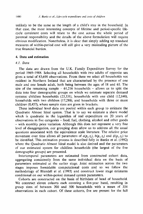
Fig. 3. Number of children in household over the life-cycle.

sample (i.e. 20 years), while young or old cohorts only exist for shorter periods at either end of the sample.

Within-period sampling error in construction of cohort averages leads to a resulting framework econometrically equivalent to errors-in-variables (though with an estimable variance-covariance structure to the measurement errors) as outlined in Deaton (1985). With sufficiently large cohort sizes, such as those here, it becomes nonetheless admissible to disregard this sampling error and treat the data as genuine panel data [see Verbeek and Nijman (1990)]. After allowing for the different periods in which each cohort is observed, and the loss of observations due to lagging the instrument set and taking first differences, the resulting dataset comprises 133 data points. For the (individual specific) real interest rate we take the after-tax Building Society lending rate if the household has a mortgage, and the borrowing rate if they do not. This interest rate is then deflated by inflation - which we define as the change in the cohort average of the non-discounted value of the individual specific linear homogeneous price index a(Pt,z,) described in the previous section.

Cohort average data for number of children and total expenditure are illustrated in figs. 3 and 4. The pattern of child bearing over the life-cycle appears from fig. 3 to be fairly stable across cohorts with little variance over the business cycle. This contrasts somewhat with the expenditure profiles in

1402 J. Banks et al., Life-cycle espendirure and costs of‘childrm

80

20 40 60 AGE OF HEAD OF HOUSEHOLD

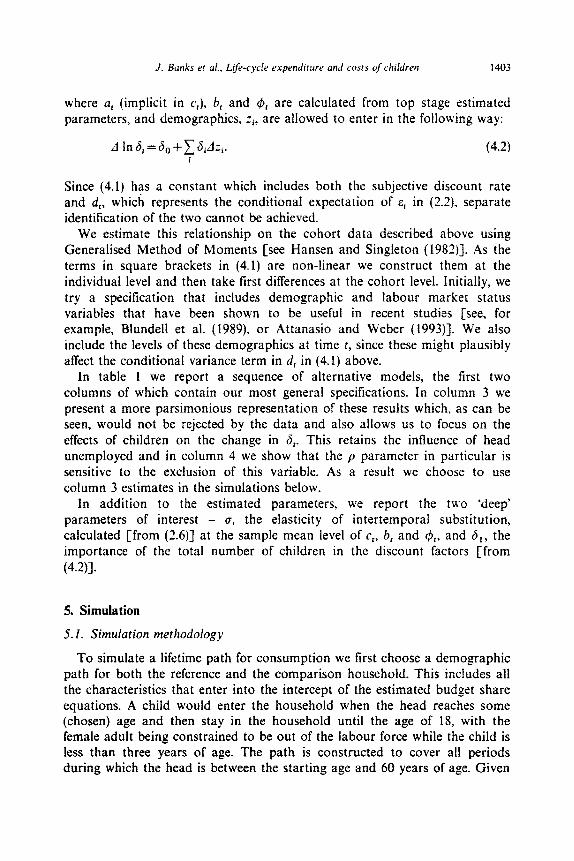
Fig. 4. Real expenditure over the life-cycle.

fig. 4 in which business cycle variation is clearly visible.‘* It should be noted that conditioning, as we do, on labour market status in the estimation of both the demand system and Euler equation may capture some of these business cycle effects.

4.2. Estimation

To estimate the intertemporal parameters that govern the evolution of dynamic expenditure paths we assume that pr is independent of demographics (i.e p,=p) which allows us to rearrange (2.7) and write down the estimable equation

=p[dlninc,dln(l+~)-dlnb,]-(*+p)dInb,+d,+r,.

(4.1)

“There is some question as to the reliability of the data underlying a sharp upturn in expenditures in the 6nal year. Consequently in these figures we plot 1969-1986 data onI>-. Even so, some cohorts can still be tracked for the full 18 years.

J. Bunks et al., Lifr-cycle e.~pendirure und costs of children 1403

where a, (implicit in c,), 6, and (p, are calculated from top stage estimated parameters, and demographics, I~, are allowed to enter in the following way:

A In dt=60 +I SiA=i. (4.2)

Since (4.1) has a constant which includes both the subjective discount rate and d,, which represents the conditional expectation of E, in (2.2). separate identi~cation of the two cannot be achieved.

We estimate this relationship on the cohort data described above using Generalised Method of Moments [see Hansen and Singleton (1982)]. As the terms in square brackets in (4.1) are non-linear we construct them at the individual level and then take first differences at the cohort level. Initially, we try a specification that includes demographic and labour market status variables that have been shown to be useful in recent studies [see, for example, Blundell et al. (1989), or Attanasio and Weber (1993)]. We also include the levels of these demographics at time t, since these might plausibly affect the conditional variance term in d, in (4.1) above.

In table 1 we report a sequence of alternative models, the first two columns of which contain our most general specifications. In column 3 we present a more parsimonious representation of these results which, as can be seen, would not be rejected by the data and also allows us to focus on the effects of children on the change in 6,. This retains the influence of head unemployed and in column 4 we show that the p parameter in particular is sensitive to the exclusion of this variable. As a result we choose to use column 3 estimates in the simulations below.

In addition to the estimated parameters, we report the two ‘deep’

parameters of interest - (r, the elasticity of calculated [from (2.6)] at the sample mean level importance of the total number of children in

(4.2~1.

5. Simulation

5.1. Simulation methodology

intertemporai substitution, of c,, b, and & and 6,, the the discount factors [from

To simulate a lifetime path for consumption we first choose a demographic path for both the reference and the comparison household. This includes all the characteristics that enter into the intercept of the estimated budget share equations. A child would enter the household when the head reaches some (chosen) age and then stay in the household until the age of 18, with the female adult being constrained to be out of the labour force while the child is less than three years of age. The path is constructed to cover all periods during which the head is between the starting age and 60 years of age. Given

1404 J. Banks et al.. Liji+cycle expenditure mri costs of children

Table 1”

(1) (2) (3) (4)

Constant

ATotkids

AHunemp

AWWife

AMortg

TotKids

Hunemp

P

Sargan d.f. Std Error of Eqn

0.0435 (0.0117)

0.2629 (0.1022)

- 1.2745 (0.6282)

0.5734 (0.4397)

-0.3612 (0.3758)

-2.5817 (0.8634)

-0.651 I (0.1716)

0.1662 (0.0776)

18.4270 16 0.0070

0.0606 0.0402 (0.03OQJ (0.0095)

0.1685 0.1903 (0.0766) (0.0826)

0.053 1 - 1.4135 (0.7170) (0.4562)

-0.0039 (0.0177)

-0.3721 (0.1718)

- 1.3357 (0.973 1)

-0.7771 (0.1914)

0.5019 (1.3387)

24.0889 16 0.0042

- 2.2264 - 1.4775 (0.7165) (0.6475)

-0.6827 -0.7604 (0.1445) (0.1309)

0.1551 0.3774 (0.0804) (0.4468)

24.7710 37.3044 18 19 0.0059 0.0054

0.02 19 (0.007 1)

1.1802 (0.0792)

“Standard errors are given in brackets. Variables are levels at time t. or lirst differences (indicated by A). Hunemp is a dummy for head of household unemployed; WWife is a dummy for working female; Mortg is a dummy for presence of a mortgage; Totkids is the total number of children of all ages. Instruments are no. of children in each of four age groups, Age of Head, Age of Spouse, Working male and Working female dummies. lending and borrowing interest rates, tenure and region dummies; all instruments are dated t - 2. D is calculated at the mean In c, for the sample of 4.76714 (at January 1987 prices).

such a profile, it is possible to construct a,, 6, and 4, for each period from the estimated ‘top stage’ parameters, and 6, and pr from the estimated Euler equation parameters.

To simulate we solve forward from the Euler equation to construct complete expenditure paths. Given the absence of an explicit solution with p#O we solve each step through iterated Nevvton-Raphson approximations to

which stems from the expression for i in periods t and t+ 1 derived as eq.

J. Banks et al., Lije-cycle expenditure and costs of children 1405

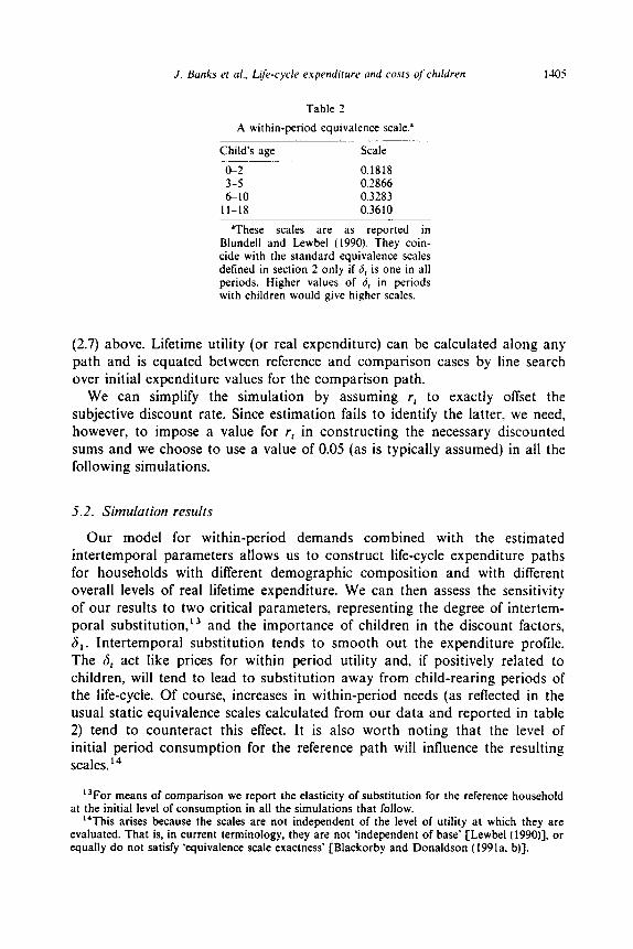
Table 2

A within-period equivalence scale.”

Child’s age Scale

ck2 0.1818 3-5 0.2866 610 0.3283

II-18 0.3610

‘These scales are as reported in Blundell and Lewbel (1990). They coincide with the standard equivalence scales detined in section 2 only if 6, is one in all periods. Higher values of 6, in periods with children would give higher scales.

(2.7) above. Lifetime utility (or real expenditure) can be calculated along any path and is equated between reference and comparison cases by line search over initial expenditure values for the comparison path.

We can simplify the simulation by assuming I, to exactly offset the subjective discount rate. Since estimation fails to identify the latter. we need, however, to impose a value for rl in constructing the necessary discounted sums and we choose to use a value of 0.05 (as is typically assumed) in all the following simulations.

S.2. Simulation results

Our model for within-period demands combined with the estimated intertemporal parameters allows us to construct life-cycle expenditure paths for households with different demographic composition and with different overall levels of real lifetime expenditure. We can then assess the sensitivity of our results to two critical parameters, representing the degree of intertemporal substitution,13 and the importance of children in the discount factors, 6,. Intertemporal substitution tends to smooth out the expenditure profile. The 6, act like prices for within period utility and, if positively related to children, will tend to lead to substitution away from child-rearing periods of the life-cycle. Of course, increases in within-period needs (as reflected in the usual static equivalence scales calculated from our data and reported in table 2) tend to counteract this effect. It is also worth noting that the level of initial period consumption for the reference path will influence the resulting scales. r4

13For means of comparison we report the elasticity of substitution for the reference household at the initial level of consumption in all the simulations that follow.

IdThis arises because the scales are not independent of the level of utility at which they are evaluated. That is, in current terminology, they are not ‘independent of base’ [Lewbel (1990)], or equally do not satisfy ‘equivalence scale exactness’ [Blackorby and Donaldson (1991a. b)].

1406 J. Bunks et al., Life-cycle expenditure and costs of‘ children

. Path-3

h

ni 20 40 60

Age Of Head Of Household Fig. 5. Life-time expenditures equivalent paths: 6, =0.155, (r= -0.683.

40 60

Age Of Head Of Household

Fig. 6. Life-time expenditure paths: 6, =0.310, CJ= -0.683.

Path-0

Path_ 1

Path-2

Path,3

Figs. 5 and 6 present comparisons of ‘life-cycle expenditure constant’ paths for households of differing demographic profiles. Using the functional form in (2.2) we take our estimate of the base elasticity of substitution and simulate expenditure paths for two different values of 6,. The reference household

J. BANS et ~1.. Q/e-cycle e.rpendirure and costs ot’children 1107

Path-0

Path-1

Path-2

Path-3

cv 20 40 60

Age Of Head Of Household Fig. 7. Life-time expenditure paths: d, =0.155, CJ= -0.622.

(Path 0) has no children at any point, but its (nominal) expenditure path slopes slightly upward. The demographics of Path 1 are identical in every way except that a child is born when the Head of Household is 26 years of age. Path 2 has two children - born when the head is 26 and 28 - and Path 3 has three children, born at the ages of 26, 28, and 30. We see that households with more children re-allocate expenditure into periods with children, and therefore (since total lifetime expenditure is constant) spend less in the periods before and after the children. Remember that we are considering anticipated changes only so, that households expecting higher costs in the future due to the presence of children will try to save in anticipation of that event. It is clear, however, that a higher value of 6, causes household re-allocation of expenditures to be more extreme.

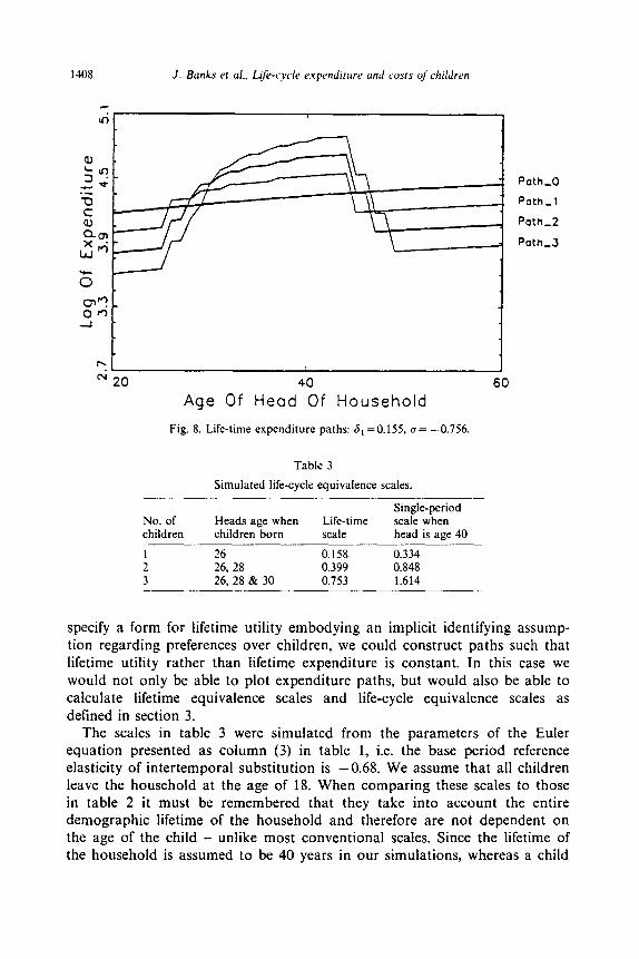
Figs. 7 and 8 present similar paths for demographic profiles with elasticities of intertemporal substitution roughly one standard deviation either side of our estimated values. Households are encouraged to substitute expenditure away from periods with children if the elasticity of substitution is large enough, and this could, in theory, be sufficiently extreme to mean that expenditure paths may actually dip as children enter the household. How- ever, in all cases that we simulate expenditure arches upward in the child- bearing periods, though for a base substitution elasticity close to - 1 (fig. 8) the comparison paths are markedly smoother as one might expect.

Finally, we turn to the calculation of equivalence scales. If we choose to

1408 J. Banks et al.. Lij>-cycle expenditurr and costs ofchildrrn

Age Of Head Of Household

Fig. 8. Life-time expenditure paths: 6, =0.155, o= -0.756.

Table 3

Simulated life-cycle equivalence scales.

No. of children

Single-period Heads age when Life-time scale when children born scale head is age 40

1 26 0.158 0.334 2 26, 28 0.399 0.848 3 26, 28 & 30 0.753 1.614

60

Poth_O

Path_ 1

Path_2

Path,3

specify a form for lifetime utility embodying an implicit identifying assumption regarding preferences over children, we could construct paths such that lifetime utility rather than lifetime expenditure is constant. In this case we would not only be able to plot expenditure paths, but would also be able to calculate lifetime equivalence scales and life-cycle equivalence scales as defined in section 3.

The scales in table 3 were simulated from the parameters of the Euler equation presented as column (3) in table 1, i.e. the base period reference elasticity of intertemporal substitution is -0.68. We assume that all children leave the household at the age of 18. When comparing these scales to those in table 2 it must be remembered that they take into account the entire demographic lifetime of the household and therefore are not dependent on the age of the child - unlike most conventional scales. Since the lifetime of the household is assumed to be 40 years in our simulations, whereas a child

J. Banks et al.. Life-cycle expenditure and costs of children 1439

is in the household for only 18 of those years, the scales in table 3 need to be more than double to be comparable with those of table 2. Of course, in constructing these scales we have made an arbitrary assumption about the household utility that cannot be captured by demand analysis. In fact the arbitrariness of any identifying assumption is highlighted in this multi-period setting since it is possible to get very different scales with reasonably similar functional forms.

6. Conclusions

Our purpose in this paper has not been to estimate a new set of equivalence scales - we have reasserted that, even within a life-cycle setting. full comparisons of inter-personal welfare are not possible from demand data alone. This point applies equally to all equivalence scales estimates based on expenditure survey data. What we have shown, however, is the importance of children in the allocation of expenditures, and therefore consumption costs. over the life-cycle. This pattern is also shown to be extremely sensitive to assumptions about intertemporal parameters. By considering the behaviour of household expenditure over time we have exploited the Euler condition to estimate such parameters of interest.

Given our discussion of the equivalence scale identification problem we would prefer to stress the simulated paths of expenditure (which are completely identified) as opposed to the utilities associated with the expenditures (which are not) as the important result of this study. Any form of equivalence scale that recognized the intertemporal aspects of household decision making would depend on the shape of these lifetime expenditure profiles. We believe that these intertemporal processes are important, and therefore for policy purposes (given the need for some monetary level of compensation) we need to look outside simple current period models and acknowledge the intertemporal factors that influence the household decision making process.

The main reason why households do not substitute expenditures over time may well not be because they are unwilling, but because they are unable. In particular this may be true at the lower end of the income distribution. where indeed our model suggests willingness to substitute may be lower anyway, and may reduce the importance of these considerations for poorer households. Arguably the most important application of the equivalence scale literature relates to the compensation of households in poverty which one might therefore think should be greater than that which the methodology of this paper would suggest. In addition, any such ‘failure’ in the market for credit (e.g. households being unable to borrow against their human capital) could be one justification for the existence of period-specific compensation such as child benetit.

1410 J. Banks er al., Lift-cycle expenditure and cosfs of children

References

Attanasio. O.P. and G. Weber, 1993, Consumption growth, the interest rate and aggregation, Review of Economic Studies 60, 631-650.

Banks, J.W., R.W. Blundell and A. Lewbel, 1992, Quadratic Engle curves, welfare measurement and consumer demand, Working paper series, no. 92/14 (Institute for Fiscal Studies, London).

Blackorby, C. and D. Donaldson, 1991a. Adult-equivalence scales, interpersonal comparisons of well-being, and applied welfare economics, in: J. Elster and J. Roemer, eds., Interpersonal comparisons and distributive justice (Cambridge University Press, Cambridge).

Blackorby. C. and D. Donaldson, 1991b. Equivalence scales and the cost of children, Discussion paper (University of British Columbia, Vancouver, BC).

Blundell, R.W. and A. Lewbel, 1991, The information content of equivalence scales, Journal of Econometrics 50, 49-68.

Blundell, R.W., M.J. Browning and C. Meghir, 1993, Consumer demand and the life-cycle allocation of household expenditures, Review of Economic Studies, forthcoming.

Blundell, R.W., P. Pashardes and G. Weber, 1993, What do we learn about consumer demand patterns from micro-data? American Economic Review 83, 576597.

Browning. M.J., 1987, Anticipated changes and household behaviour: A theoretical framework, Working paper (McMaster University, Hamilton, Ont.).

Browning, M.J., 1989, The intertemporal allocation of expenditure on nondurables, services and durables, Canadian Journal of Economics 22, 22-36.

Browning, M.J., 1991, Children and household economic behavior, Journal of Economic Literature.

Deaton, AS., 1985, Panel data from time series of cross sections, Journal of Econometrics 30, 109-126.

Gorman. 1959, Separable utility and aggregation, Econometrica 27, 469-481. Hall, R.E., 1978, Stochastic implications of the life-cycle permanent income hypothesis: Theory

and evidence, Journal of Political Economy 86, 971-988. Hansen, L.P. and K.J. Singleton, 1982, Generalised instrumental variable estimation of non-

linear rational expectations models, Econometrica 50, 1269-1286. Keen, M.J., 1990, Welfare analysis and intertemporal substitution, Journal of Public Economics

42, 47-66. Lewbel, A., 1988, Quadratic logarithmic Engel curves and the rank extended translog, Working

paper no. 231 (Brandeis University, Waltham, MA). Lewbel, A., 1990, Household equivalence scales and welfare comparisons, Journal of Public

Economics 39, 377-39 I. MaCurdy, T.E., 1983, A simple scheme for estimating an intertemporal model of labour supply

and consumption in the presence of taxes and uncertainty, International Economic Review 24, 265-289.

Moffttt, R.. 1989, Estimating dynamic models with a time series of repeated cross-sections, Journal of Econometrics.

Pashardes, P., 1991, Contemporaneous and intertemporal child costs: Equivalent expenditures vs. equivalent income scales, Journal of Public Economics 45, 191-213.

Pollak, R.A. and T.J. Wales, 1979, Welfare comparisons and equivalence scales, American Economic Review 69, 216221.

Verbeek, M. and T. Nijman, 1990, Can cohort data be treated as genuine panel data?, Mimeo. (Tilburg University, Tilburg).

Documents

Life-cycle expenditure allocations and the consumption costs of …uctp39a/BanksBlundellPrestonEEA... · 2011-03-20 · European Economic Review 38 (199-t) 1391-1410. North-Holland