CAIT-UTC-013

Life Cycle Assessment of Asphalt Pavement

Maintenance

FINAL REPORT January 2014

Submitted by: Hao Wang

Assistant Professor

Rashmi Gangaram Graduate Research Assistant

Center for Advanced Infrastructure & Transportation Rutgers, The State University of New Jersey

100 Brett Road, Piscataway, 08854

External Project Manager Sue Gresavage

New Jersey Department of Transportation

In cooperation with

Rutgers, The State University of New Jersey And

State of New Jersey Department of Transportation

And U.S. Department of Transportation Federal Highway Administration

2

Disclaimer Statement

The contents of this report reflect the views of the authors,

who are responsible for the facts and the accuracy of the

information presented herein. This document is disseminated

under the sponsorship of the Department of Transportation,

University Transportation Centers Program, in the interest of

information exchange. The U.S. Government assumes no liability for the contents or use thereof.

3

1. Report No.

CAIT-UTC-013

2. Government Accession No. 3. Recipient’s Catalog No.

4. Title and Subtitle

Life Cycle Assessment of Asphalt Pavement Maintenance

5. Report Date

January 2014 6. Performing Organization Code

CAIT/Rutgers University

7. Author(s)

Hao Wang, Rashmi Gangaram

8. Performing Organization Report No.

CAIT-UTC-013

9. Performing Organization Name and Address

Center for Advanced Infrastructure and Transportation

Rutgers, The State University of New Jersey

96 Frelinghuysen Road, Piscataway, 08854

10. Work Unit No.

11. Contract or Grant No.

DTRT12-G-UTC16

12. Sponsoring Agency Name and Address 13. Type of Report and Period Covered

Final Report 09/01/2012 – 12/31/2013

14. Sponsoring Agency Code

15. Supplementary Notes

U.S. Department of Transportation/Research and Innovative Technology Administration

1200 New Jersey Avenue, SE

Washington, DC 20590-0001

16. Abstract

This study aims at developing a life cycle assessment (LCA) model to quantify the impact of pavement preservation

on energy consumption and greenhouse gas (GHG) emissions. The construction stage contains material,

manufacture, transportation and placement phases. The Highway Development and Management (HDM-4) model

and the Motor Vehicle Emission Simulator (MOVES) were used to analyze fuel consumption and emissions treated

by different preservation treatments. Surface characteristics such as roughness, texture and deflection were taken

into account in tire rolling resistance. The thin overlay was found to have the highest energy consumption and

emissions among four preservation treatments during construction stage, but at the same time resulted in the greatest

reduction of energy and emission at usage stage. If only construction stage is considered, energy and emissions are

ruled by use of amount of material and manufacture process. The reductions of GHG emission at usage stage are

much greater than the GHG emission produced at construction stage for all preservation treatments. Excluding the

usage stage will omit the fact that construction stage has less impact on pavement LCA than usage stage. The study

results provide valuable insights in selecting sustainable pavement maintenance strategies from an environmental

view point.

17. Key Words

Life Cycle Assessment; Pavement Preservation; Construction

Stage; User Stage

18. Distribution Statement

19. Security Classification (of this report)

Unclassified 20. Security Classification (of this page)

Unclassified 21. No. of Pages

67 22. Price

Center for Advanced Infrastructure and Transportation

Rutgers, The State University of New Jersey

100 Brett Road

Piscataway, NJ 08854

Form DOT F 1700.7 (8-69)

T E C H NI C A L R E P OR T S T A NDA RD TI TLE P A G E

4

Table of Contents

Chapter 1 INTRODUCTION ......................................................................................................... 8

1.1 Background ............................................................................................................................ 8

1.2 Problem Statement ............................................................................................................. 10

1.3 Objective ............................................................................................................................. 10

1.4 Outline of Report ................................................................................................................. 11

Chapter 2 LITERATURE REVIEW ............................................................................................... 12

2.1 LCA Overview ...................................................................................................................... 12

2.2 LCA Approaches ................................................................................................................... 13

2.3 LCA Studies on Pavement Type Selection ........................................................................... 14

2.4 LCA Studies on Sustainable Pavement Materials ................................................................ 19

2.5 LCA Studies on Pavement Maintenance and Preservation ................................................. 21

2.6 Summary ............................................................................................................................. 24

Chapter 3 EMISSION AND ENERGY AT CONSTRUCTION STAGE .............................................. 25

3.1 Pavement Preservation Treatments ................................................................................... 25

3.2 Life Inventory Data .............................................................................................................. 26

3.3 Energy and Emission of Different Preservation Treatments............................................... 31

Chapter 4 EMISSION AND ENERGY AT USAGE STAGE OF PAVEMENT .................................... 34

4.1 MOVES (Motor Vehicle Emission Simulator) Overview ...................................................... 34

4.2 Consideration of Road Surface Characteristics in MOVES .................................................. 35

4.3 Pavement Factors Affecting Vehicle Emission and Energy ................................................. 37

4.4 Summary ............................................................................................................................. 43

Chapter 5 LIFE-CYCLE ENERGY AND EMISSIONS OF PAVEMENT PRESERVATION ................... 44

5.1 Effect of Preservation on Pavement Roughness ................................................................. 44

5.2 Effect of Pavement Preservation on Energy and Emissions at Usage Stage ....................... 46

5.3 Life-Cycle Emission and Energy ........................................................................................... 48

5.4 Effect of Preservation on User Costs ................................................................................... 50

5.5 Effect of Pavement Preservation on Emission Cost ............................................................ 55

5

5.6 Summary ............................................................................................................................. 57

Chapter 6 CONCLUSIONS AND RECOMMENDATIONS ............................................................. 58

6.1 Major Findings ..................................................................................................................... 58

6.2 Future Research Recommendations ................................................................................... 59

REFERENCES .................................................................................................................................. 60

6

LIST OF FIGURES

Figure 2.1 Life Cycle Assessment Framework ............................................................................... 12

Figure 4.1 Effect of MTD on Energy and Emission ........................................................................ 38

Figure 4.2 Effect of IRI on Energy and Emission ........................................................................... 40

Figure 4.3 Effect of Deflection on Energy and Emission ............................................................... 42

Figure 5.1 Roughness data at Site 17 from LTPP- SPS3 ................................................................ 45

Figure 5.2 Roughness Data at Site 27 from LTPP- SPS3 ................................................................ 46

7

LIST OF TABLES

Table 3.1 Percentage Passing For Different Sieve Size for Slurry Seal Type I, II and III

(Maintenance Technical Advisory Guide (MTAG)) ....................................................................... 26

Table 3.2 Energy Data for Construction Materials and Processes................................................ 29

Table 3.3 Emission Data for Construction Materials and Processes ............................................ 30

Table 3.4 Energy Consumption and Emission for One Lane-Mile HMA Overlay .......................... 31

Table 3.5 Energy Consumption and Emission for One Lane-Mile Slurry Seal .............................. 32

Table 3.6 Energy Consumption and Emission for One Lane-Mile Chip Seal ................................. 32

Table 3.7 Energy Consumption and Emission for One Lane-Mile Crack Seal ............................... 33

Table 4.1 Parameters for CR2 model in HDM 4 Model ................................................................ 37

Table 4.2 Sensitivity Analysis of Energy Consumption at Different MTDs ................................... 38

Table 4.3 Sensitivity Analysis of Emission at Different MTDs ....................................................... 39

Table 4.4 Sensitivity Analysis of Energy Consumption at Different IRIs ....................................... 40

Table 4.5 Sensitivity Analysis of Emission at Different IRIs .......................................................... 41

Table 4.6 Sensitivity Analysis of Energy Consumption at Different Deflections .......................... 42

Table 4.7 Sensitivity Analysis of Emission at Different Deflections .............................................. 43

Table 5.1 Energy Consumption in MJ during Usage Stage ........................................................... 46

Table 5.2 Energy Consumption Using Truck Percentage during Usage Stage .............................. 47

Table 5.3 Emission Values with Truck Percentage during Usage Stage ....................................... 47

Table 5.4 Change of Energy and Emission after Pavement Preservation for Site 17 ................... 49

Table 5.5 Change of Energy and Emission after Pavement Preservation for Site 27 ................... 50

Table 5.6 Effect of Roughness on Fuel Consumption Cost ........................................................... 51

Table 5.7 Effect of Roughness on Repair and Maintenance Cost ................................................. 52

Table 5.8 Effect of Roughness on Tire Wear Costs ....................................................................... 52

Table 5.9 User Costs Analysis for Site 27 ...................................................................................... 53

Table 5.10 User Costs Analysis for Site 17 .................................................................................... 54

Table 5.11 User Cost Saving by 10 Million Vehicles for Site 27 .................................................... 54

Table 5.12 User Cost Saving by 10 Million Vehicles for Site 17 .................................................... 54

Table 5.13 Urban Emission Cost in Dollars per Ton by Kendall et al (2005) ................................. 55

Table 5.14 Emission Cost at Usage Stage for Site 27 and Site 17 ................................................. 56

Table 5.15 Emission Cost at Construction Stage........................................................................... 56

Table 5.16 Cost Saving for Site 27 and Site 17 With 10 Million Annual Traffic ............................ 57

8

Chapter 1 INTRODUCTION

1.1 Background

The basic definition of sustainability includes three interrelated elements: economy, environment

and society. As the importance of environmental sustainability becomes increasingly

recognized, public agencies and private contractors are embracing the need to adopt

sustainable products, processes, and technologies in all aspects of building and infrastructure.

With regards to transportation infrastructure, this includes the consideration of sustainability in

the design, construction, operation, and maintenance of highways, airports, and railroad,

including pavements.

There are approximately 4.2 million kilometers (2.6 million miles) of paved public roads

in the United States, including concrete and asphalt pavements. Pavements pose a particular

challenge to achieving the goal of sustainable transportation infrastructure because the

construction and maintenance of pavements requires the consumption of large quantities of

non-renewable materials and creates significant energy and environmental impacts. For

example, 320 million metric tons (350 million tons) of raw materials go into the construction,

rehabilitation, and maintenance of pavements annually in the United States (Holtz and Eighmy

2000).

A sustainable pavement comes with the combination of durability, cost effectiveness,

eco-efficiency and high performance. Many sustainable practices have been implemented in

pavements through improved or innovative design and the utilization of recycled material and

industry by-products. For example, long-lasting pavements are designed to increase

sustainability through long service lives, minimum maintenance and repair, and reduced traffic

disruptions. Porous pavements have been designed to reduce the need for storm-water

retention basins and improve the quality of storm-water runoff. As another example, recycled

asphalt pavement (RAP) and recycled asphalt shingles (RAS) are becoming commonly recycled

materials in flexible pavements to reduce construction costs and the use of non-renewable

resources. Similarly, the increasing use of high percentages of supplementary cementitious

materials (SCMs) in rigid pavements cannot only recycle the waste material but also replace

cement in the concrete mix that is very energy intensive and emits significant greenhouse gas

(GHG) emissions. Recently, the use of warm mix asphalt (WMA) has been promoted because

9

of its energy and environmental benefits brought by the lowered production and placement

temperatures.

Despite that a lot of sustainable practice has been implemented in the pavement system, an

assessment tool to properly quantify environmental sustainability in the pavement system is still

missing and required. There are currently a number of gaps in measurement and quantification

of the on-going sustainable activities that make it difficult to include sustainability as an

integrated part in the decision-making process for public agencies or private contractors.

Furthermore, the pavement system contributes directly to vehicle operating costs and fuel

economy due to the rolling resistance at tire-pavement interface, which also affects GHG

emissions significantly. In 2008, the road transport produced 33 percent of the GHG emissions

in the U.S. (1,946 million tons of carbon dioxide equivalent [CO2eq]), second only to that

produced by the electrical power generation industry (EPA 2010). Therefore, a refined

systematic approach for a pavement system is needed to quantify the environmental impacts of

the pavement system during its whole life cycle including the usage stage.

In the building industry, the U.S. Green Building Council’s LEED certification program

provides building owners and operators with a framework for identifying and implementing

practical and measurable green building design, construction, operations and maintenance

solutions. Recently, rating systems have been developed to promote green highway

construction, such as Greenroad (University of Washington), GreeLITES (New York DOT),

GreenPave (Ontario Ministry of Transportation), and INVEST (FHWA). However, these rating

systems mainly focus on design and construction elements of highways. Specific methods are

still needed to quantify the impacts that the pavement system may have on urban or rural

environments and on the energy sector.

Life Cycle Assessment (LCA) is an analytical technique for assessing potential

environmental burdens and impacts throughout a product’s life from raw material acquisition

through production, use and disposal (ISO 2006). LCA is an appropriate tool for assessing the

environmental impacts and helps to identify which impacts are the most significant across the

life cycle. It provides metrics that can be used to measure progress toward environmental

sustainability. Therefore, a systematic approach is needed to evaluate the environmental

impacts of pavement system on its whole life cycle.

As such, the LCA should be based on an understanding of all the pavement-related

processes, including material extraction and processing, construction, operation, preservation,

rehabilitation, and disposal that go into all phases of the life cycle of pavement. The impact of in-

10

service use of the pavement on the environment and on society - including vehicle operations,

surface run-off, urban heat island effect, noise, and emissions - is of critical importance and

should be considered.

1.2 Problem Statement

Construction, rehabilitation, and maintenance of highway pavements require obtaining,

processing, transporting, manufacturing, and placement of large amounts of construction

materials. A better pavement comes with the combination of durability, cost effectiveness, eco-

efficiency and high performance. Many practices have been implemented in pavement

construction to increase the sustainability of pavement through reduced energy consumption

and utilization of recycled material and industry by-products.

The Federal Highway Administration (FHWA) has started to increase the focus on

preservation and to address the deterioration of the nation’s highways. Compared to

rehabilitation, preventive maintenance treatments mainly focus on surface refreshment to

alleviate functional indicators of pavement deterioration such as friction, minor cracking or oxide

of the asphalt pavement, rather than structural deterioration. Preventive maintenance can be

used to prevent minor deterioration, retard pavement failures, and reduce the need for

corrective maintenance or rehabilitation and thus prolong pavement service life.

The economic and environmental impacts of different pavement maintenance and

preservation activities are important for the selection of pavement repair alternatives. A lot of

studies have been conducted to evaluate the cost-effectiveness of pavement preservation using

life cycle cost analysis (LCCA) (Chan 2007). However, little research has been conducted to

evaluate and select appropriate pavement maintenance treatments considering its energy and

environmental impacts. Pavement maintenance projects consume massive amounts of

nonrenewable resources and energy and generate greenhouse gas (GHG) emission. The

various maintenance techniques also provide different pavement surface conditions that affect

the usage cost of vehicle operation. Therefore, a systematic approach is needed to evaluate the

environmental impacts of pavement maintenance at its whole life cycle.

1.3 Objective

Life Cycle Assessment (LCA) is an analytical technique for assessing potential environmental

burdens and impacts throughout a product’s life from raw material acquisition through

production, use and disposal. LCA is an appropriate tool for assessing the environmental

impacts and helps to identify which impacts are the most significant across the life cycle. The

main research objective is to develop a LCA methodology to consider the energy and

11

environmental impacts of pavement maintenance at its construction and usage stage, which can

be used by state agencies for the appropriate selection of a maintenance strategy.

The general process, methodology, and state of practice of LCA and the application of

LCA in pavement including both the construction and usage phases are reviewed. Different

types of pavement maintenance and preservation treatments consume different amounts of

energy and produce GHG emissions. Maintenance treatments considered in this study included

thin hot-mix asphalt (HMA) overlay, chip seal, slurry seal and crack seal. The analysis of energy

and GHG emissions considered the entire process for each treatment, including raw materials,

construction, service life extension, and the usage stage as appropriate. Particularly, the

effectiveness of pavement maintenance on pavement roughness is investigated using the data

in the long-term pavement performance (LTPP) database for analyzing the effect of pavement

maintenance on vehicle fuel consumption and pollutant emission.

1.4 Outline of Report

This report is divided into six chapters. The first chapter introduces the background, problem of

statement, and objective. The second chapter summarizes the literature review of various LCA

studies on pavement type selection, sustainable pavement materials, and pavement

maintenance and preservations. The third chapter compares energy consumption and pollutant

emission of four preservation treatments at the construction stage. The fourth chapter quantifies

energy consumption and pollutant emission of four preservation treatments at the usage stage

considering the effect of pavement preservation on tire-pavement rolling resistance. The

combined life-cycle energy consumption and pollutant emission at construction and usage

stages are calculated. The final chapter presents the analysis’ findings, conclusions and future

study recommendations.

12

Chapter 2 LITERATURE REVIEW

2.1 LCA Overview

Life Cycle Assessment (LCA) is a technique to assess environmental effects associated with a

product’s life cycle. This technique starts with the start of a product/process and finishes with

the end of the product/process. It includes raw material extraction, material production,

processing, manufacturing, distribution, transportation, maintenance, and disposal/recycle (ISO

1997).

The formal structure of LCA was framed by International Standards Organization (ISO).

It shows three basic stages: Goal and scope definition, inventory analysis, impact analysis as

shown in Figure 2.1.

Figure 2.1 Life Cycle Assessment Framework

(Adapted from ISO 14040)

Goal Definition and Scope

The first and basic step in LCA is definition of goal and scope of the process. In any process for

LCA consideration, the goal is to quantify and characterize the flow of all the materials involved

in the process which helps in identifying the environmental impact of the material and find an

alternative approach to reduce the impact. LCA has emerged as a widely practiced process to

reduce the harmful environmental effects and it has given many beneficial results. Defining the

goal of any process is considered to be the most critical step in beginning a LCA evaluation.

Goal, Definition

& Scope

Inventory

Analysis

Impact

Assessment

Interpretation

13

Goal is to define the questions that are to be answered followed by choosing the evaluation’s

scope. Scope includes defining what and how the whole process will be portrayed, what

alternatives need to be defined. The assessment of the resources should also be done which

can also be applied to analysis. This step involves defining the system boundaries, assumptions

and limitations of the system.

Inventory Analysis

The next stage following goal and scope definition is inventory analysis, sometimes also known

as life cycle inventory (LCI). Inventory analysis is analyzing an inventory flow for a product or

process from cradle stage to end stage. It includes inputs from water, energy and raw materials

to air water and soil. Inventory model is constructed as a flow chart and it includes input and

output data about the system being considered, a flow model is made using the data of the

technical system. These data are collected according to the technical system boundaries. Data

consists of products initial form as raw material to the end of life/recycle stage. Data is directly

related to the goal defined for the LCA.

Impact Assessment

LCA’s impact assessment constitutes of influences of the activities conducted by LCA inventory

analysis on specific environmental properties and relative seriousness of the changes in the

affected environmental properties. Assessing environmental impact of process is a complicated;

but it can be performed by employing relationships between environment and elements affecting

the environment, which are the items listed in the inventory analysis that have potential to

produce harmful effects to the environment. The relationships between stressors (element

producing stress to a system) and environment can be developed by combining LCA inventory

results with its effects.

As the name ‘impact’ suggests, this step assesses impact of any product and process on

environment and human health. The assessment categories include global warming potential,

acidification, eutrophication, criteria air pollutants, photochemical smog and etc.

2.2 LCA Approaches

There are three major types of LCA models which depends on the source of information used in

the LCA process. The first is Economic Input-Output model (EIO), known as EIO-LCA, which is

developed by Carnegie Mellon University.

14

The Economic Input-Output Life Cycle Assessment (EIO-LCA) method is used to

estimate the materials and energy resources required activities and the environmental

emissions resulting from, activities in our economy. This method uses transactions done by

industries, like one industry buying from other industries and information about each involved

industry’s environmental emissions to calculate the total emission throughout the supply chain.

This method can be applied to any transactions between industries related to the economy of

the sectors.

The second is process-based LCA which is based on the methodology set by

International Standards Organization (ISO) 14040 and 14044 for LCA and known as ISO-LCA

too. In process based LCA, specific process data and a computational tool or matrix analysis is

used to form a model for the assessment of the process. The third method is called Hybrid LCA

in which an EIO model is integrated with process based data to produce more comprehensive

representations for environmental effects of the processes (Greenroads Manual v1.5).

2.3 LCA Studies on Pavement Type Selection

Pavements have been divided into two broad categories including rigid and flexible pavements.

A flexible pavement consists of a wearing surface of asphalt concrete built over a base course

and a sub-base course. Base and Sub-base courses are generally made up of granular material

and rest on the compacted subgrade. A rigid pavement consists of concrete slabs placed on

base course and subgrade. Flexible pavement has better ability to ride and lower noise, while

rigid pavement has greater rigidity and stiffness. Concrete pavements usually comprise of less

layers and total thickness than asphalt pavements.

Previous LCA studies on pavements focused on comparing the impacts of two or more

alternative designs often asphalt versus concrete.

A study of LCA of asphalt and concrete pavements was performed by Athena Institute

(2006). This study presented embodied primary energy and global warming potential (GWP)

over an analysis period of 50 years for the construction and maintenance of asphalt and

concrete alternatives. The design alternatives include pavement structures respectively using a

200-mm concrete slab and a 175-mm asphalt layer. All pavement designs were developed

using the AASHTO 1993 design method and Cement Association of Canada design method.

The study did not include traffic operational considerations. Feedstock energy was considered

in the analysis for asphalt. Feedstock energy is the chemical energy stored in material when not

in use, it is considered as a part of embodied energy (Santero et al., 2011). Results show that

the asphalt pavement consumes greater energy than the concrete pavement. The feedstock

15

energy was found to have the highest contribution to the total energy for asphalt pavements.

The GHG emissions are in higher values for concrete alternatives than asphalt alternatives.

Said et al. (2011) presented a tool developed by the Athena Sustainable Material

Institute and Morrison Hershfield that is called the ATHENA Impact Estimator for Highways for

LCA. It was found that asphalt pavement had approximately 83% more global-warming potential

(GWP) effect during the rehabilitation stage as compared to the concrete pavement. Results

suggest that the flexible pavement embodies approximately 2.9 times more primary energy than

the rigid pavement.

Chan (2007) built a Life Cycle Inventory (LCI) to develop the environmental impacts of

asphalt and concrete alternatives. Material production and waste treatment; material

transportation to and from construction site; and construction and maintenance process are the

activities for road construction/rehabilitation considered as system boundaries in this study. The

environmental impacts of asphalt and concrete alternatives for 13 highway construction

rehabilitation projects were computed in Michigan. The results included the impacts from

construction, maintenance and equipment process and shows that concrete alternatives had

higher GHG emissions than asphalt alternatives. The primary energy consumption of asphalt

pavements is higher than concrete pavements and also the reconstruction process has yielded

more GHG emissions than the rehabilitation process.

Hakkinen and Makela (1996) performed a similar study comparing stone-mastic asphalt

(SMA) and jointed plain reinforced cement concrete (JPCP). They used a process-based LCA

considering each phase of the life cycle of pavement excluding end of life module. Both types of

pavements were evaluated using 18 different environmental criteria including CO2 emissions,

energy consumption, air pollutants. The construction phase includes fuel consumption and

onsite paving equipment and does not consider traffic delays as it assumes completely new

pavement construction. They concluded that the concrete pavement produced 40-60% more

CO2 emission as compared to the asphalt pavement.

Horvath and Hendrickson (1998) performed a study using EIO-LCA developed by

Carnegie Melon University to compare the energy consumption of hot-mix asphalt (HMA) and

continuously reinforced concrete pavement (CRCP). This study focused on extraction and

production of different surface materials and qualitative analysis of construction phase and end

of life. It did not consider feedstock energy of asphalt and concluded that the asphalt pavement

consumes 40% more energy than the concrete pavement.

Roudebush (1999) compared concrete and asphalt pavements. They emphasized on

emergy which is explained as a summation method for life cycle energy consumption to

16

accommodate the quality and source of energy. A 24-feet wide and 3281-feet long pavement

section was analyzed for a period of 50 years. Roudebush examined materials, construction,

maintenance and end-of-life phases in this study, ignoring the use phase completely. This report

concluded that the asphalt pavement structure requires 90.8% more energy than the concrete

pavement. This huge difference is because emergy transformity for asphalt is double that of

concrete per mass of material. Transfromity is explained to convert different types of energy into

their solar energy equivalents and named as solar emjoules. Transformity calculation is not

included in the report.

Berthiaume and Bouchard (1999) compared asphalt and concrete pavements by using a

criteria called exergy. Exergy is a form of energy which is available to be used and even after

system and surroundings reach equilibrium. Exergy can also be explained as a measurement of

the work and accounts for differences in energy quality. It was concluded that concrete has

higher exergy consumption for the three traffic levels -residential, urban and highways when

compared to asphalt. This study had a narrow approach as it neglects construction, use and

end of life phases and only considers the material production phase.

Mroueh et al., (2000) examined seven structures that used coal ash, crushed concrete

waste, and blast furnace slag as substitutes for virgin materials. This study considered material,

construction and maintenance phases, excluding use and end of life phases. This allowed

combining all environmental burdens together into a single score. This report concludes energy

and air emissions, raw materials, leaching water use and noise effect.

Stripple (2001) performed a study on a jointed plain concrete pavement (JPCP) and

asphalt pavements constructed using hot and cold production techniques respectively. The

study considered several environmental metrics, including energy consumption, various water

and air pollutants, waste generation, and resource consumption. This study concludes that

without feedstock energy, JPCP consumes more energy than asphalt pavements. The CO2

emission results are same between JPCP and asphalt pavements.

Nisbet et al., (2001) compared an asphalt pavement to a doweled JPCP pavement for

urban collector and highway routes. They compared energy consumption, various air emissions

like particulate matter, CO2, SO2, NOx etc. This study included all the phases except the use

phase. They concluded that for the urban collector and highway scenarios, concrete pavements

require less overall material and have a lower embodied primary energy, and thus produce

lower air emissions, it includes the feedstock energy in bitumen.

17

Park et al., (2003) used a hybrid LCA method to analyze asphalt concrete and ready mix

concrete, because this study lacks data and documentation so it becomes difficult to interpret

and firm result from the study. All the phases except use phase were included in the study.

Treloar et al. (2004) performed a hybrid LCA analysis on eight pavement types including

a CRCP, an un-doweled JPCP, a composite pavement and various asphalt pavements. Study

includes materials, construction, use and maintenance and rehabilitation phases and excludes

end of life phase. They concluded that the un-doweled JPCP had the lowest energy input, while

the full depth asphalt had the highest energy input.

Zapata and Gambatese (2005) analyzed the materials production and construction

phases of the life cycle for energy consumption of a CRCP and an asphalt pavement. The study

thoroughly analyzed each process associated with materials extraction, manufacturing, and

construction by collecting energy data from various studies. This study concluded that the

CRCP consumed the most energy over material extraction and construction phases, which

supports the result drawn by Stripple (2001).

Various literatures suggest that rigid pavements provide better fuel efficiency than

flexible pavements. A flexible pavement consists of various layers – the sub-base, base course

intermediate course, surface course and sometimes a friction course. A rigid pavement is

composed of Portland cement concrete placed on granular sub-base. As flexible pavements

have less flexural strength compared to rigid pavements, they are deflected more as vehicle

pass overhead, thus absorbing energy that would otherwise be used for accelerating the vehicle

(Zaniewski, 1989).

Zainewski et al. (1982) evaluated various factors that influence vehicle fuel consumption

such as speed, grade, curves, pavement condition, and pavement type. Fuel consumption

reading were performed on eight vehicles, tests were done at 10 mph to 70 mph on 12

pavement sections. This study focused on the impact of pavement type (asphalt, Portland

cement concrete, and gravel) on fuel consumption. Changes were found in fuel consumption

between asphalt and concrete pavement up to 20%.

Ardekani and Sumitsawan (2009) used two pairs of asphalt and concrete pavements

with identical gradient and roughness measurements to perform fuel consumption

measurements for two driving conditions (constant speed of 48 km/h (30 mph) and acceleration

from stand still). It was concluded that passenger vehicles used significantly less fuel on

concrete pavements compared to asphalt pavements. Fuel consumption rates per unit distance

were lower for Portland cement concrete (PCC) pavement at all times. A saving of 3% to 17%

was recorded on the PCC pavement.

18

Zaabar and Chatti (2010) performed tests to determine the impact of pavement type on

fuel consumption in U.S. conditions. The authors used five vehicles (passenger car, van, SUV,

light truck, articulated truck) at speeds of 56 km/h (35 mph), 72 km/h (45 mph) and 88 km/h (55

mph). They determined that only a change in fuel consumption of light and articulated trucks in

summer conditions and at low speed could be detected between pavement types. The change

in fuel consumption between asphalt and concrete pavement was found around 5%. They

concluded that although pavement structure appeared to play a role in fuel consumption

differences were only measurable for heavy vehicles travelling at low speeds during

summertime conditions.

Milachowski et al. (2012) studied the environmental impact of concrete and asphalt

pavement for motorway construction and maintenance. A usage period of 30 years was

considered for the pavements with normal traffic conditions. Two maintenance conditions were

taken into account (minimum and maximum maintenance scenarios). By comparing all the

impact categories it is deduced that that the maintenance measures applied on both pavements

for rehabilitation show much less environmental impact for the concrete pavement than for the

asphalt pavement. The largest potential impact reduction lies in lowering fuel consumption since

the impact is mainly due to the combustion of fossil fuel. Both concrete and asphalt pavements

show similar environmental impacts on GWP. They concluded that the potential environmental

impact due to traffic is 100 times more than construction and maintenance together.

American concrete pavement association (ACPA) (2002) studied albedos of pavement

surfaces according to pavement types. Albedo is the ratio of reflected solar radiation back to

the total amount of radiation falling on the surface. A perfect absorber has an albedo value of

zero and perfect reflectors have value of 1. It is concluded in the report that concrete material

affects the reflectance of the concrete pavements. Asphalt surfaces are not very good reflectors

because of the color of the materials. Concrete pavements can be made a better reflector by

using white cement and lighter aggregate.

Researches by Adrian and Jobanputra (2005) suggested that asphalt pavements

required almost 50% more lighting power than concrete pavements to achieve proper

illumination. Asphalt pavements require more lighting than concrete pavements as the color of

the structure plays an important role. Reflectance property of aged pavements may become

moderate as asphalt pavement gets lighter with the time while concrete pavement gets darker.

AASHTO (2005) roadway lighting design guide recommends that asphalt pavements need

approximately 33%-50% more light power than concrete pavements to achieve sufficient

illumination (Santero et al., 2011).

19

2.4 LCA Studies on Sustainable Pavement Materials

A handful of studies have used LCA or similar techniques to evaluate the environmental impacts

of using by-products and recycled materials in pavements. These waste streams include

products such as foundry slag, bottom ash, fly ash, reclaimed asphalt pavement (RAP),

shredded rubber tires, crushed glass, plastics, and crushed concrete.

Reclaimed asphalt pavement (RAP) is the removed and/or processed materials containing

asphalt and aggregates. These materials are generated when asphalt pavements are removed

for construction, resurfacing, or to obtain access to buried utilities. When properly crushed and

screened, RAP consists of high-quality, well-graded aggregates coated by asphalt cement.

There are many advantages in using RAP in new mixtures like environmental friendliness and

higher resistance to some type of pavement distress.

Copple et al. (1981) studied the energy saving by the use of recycled concrete in new

concrete. They concluded that based on a 15-mile hauling distance for virgin aggregate when

compared to concrete with virgin aggregate, and concrete with RCA save 10% energy.

Chui et al., (2007) performed a study to evaluate the environmental impact of

rehabilitating pavement using different recycled materials that are traditional hot-mix asphalt,

RAP, asphalt rubber, and glassphalt. This analysis indicated that the reduction of the amount of

asphalt and the consumption of heat were the main factors to lower the eco-burden of

rehabilitation work. The amount of reduced or increased asphalt usage can also affect the

service life of pavement. Just reducing the amount of asphalt without considering its effect on

pavement life would increase the amount of rehabilitation work and increase the eco-burden.

This study concluded that using recycled hot mix asphalt could reduce the eco-burden by 23%;

while Glassphalt increased the eco-burden by 19%. The majority of eco-burden came from two

sources that were asphalt and heat required.

Lee et al. (2011) used PaLATE to quantify the energy consumption and GHG emissions

of RAP. RAP was milled from existing pavements and reused in new mixtures by proper curing

and sieving. In this study, the life cycle of pavement was divided into four parts: materials

manufacture; construction; maintenance and operation; and rehabilitation or reconstruction. The

environmental impact of using different percentages of RAP in the asphalt mixture was

evaluated using PaLATE. The information needed to calculate energy emissions and GHG

emissions includes the amount of material transported to and from construction site, material

20

production and also the transport of recycled material to the manufacturing plant. Results show

that 30% RAP content only requires 84% energy consumption and 80% GHG emissions higher

the RAP content higher the environmental benefits can be obtained.

Lie and Wien (2011) evaluated costs, energy and greenhouse gas emissions of different

base materials that were used in the test road cells built on MnROAD facility in Minnesota. The

test cells have same asphalt layer, sub-base courses, sub grade but different bases courses

such as the untreated recycled pavement materials (RPM), conventional crushed aggregate,

and cementitious high carbon fly ash (CHCFA) stabilized RAP. The life cycle analysis indicates

that the cost, energy and GHG emission impacts. The energy and greenhouse emissions are

evaluated using PaLATE. The energy consumption consists of consumption of construction

energy, transportation energy and processing energy. The GHG emissions were converted to a

direct Global Warming Potential (GWP) using the well accepted CO2 equivalence method

developed by International panel on climate change. The LCA results indicate that the usage of

fly ash stabilized RPM as base course in flexible pavements can significantly reduce the life

cycle cost, energy consumption, and GHG emissions compared to the untreated RPM and

conventional crushed aggregate.

Kalman (2013) did the study with an aim of developing innovative technologies for end of

life strategies for asphalt road by recycled asphalt. LCA methodology was used to analyze the

environmental impacts of different materials. The life cycle includes installation, maintenance,

use and deconstruction of asphalt. Aim of this project is to analyze the environmental criteria

like assessment of risks and benefits to the environment with use of the recycled asphalt.

Use of warm mix asphalt (WMA) has grabbed attention in asphalt industry to reduce

energy consumption and air emissions (Hasan, 2009). By using WMA additives, the viscosity of

asphalt binder can be reduced and asphalt mixture can be compacted and paved at cooler

temperatures. Warm mix asphalt can be made by adding asphalt emulsion, waxes or water to

asphalt binder prior to mixing. When compared to HMA, WMA allows production and placement

of asphalt paving at cooler temperature. Composition of WMA is same as HMA except the

additive added to lower the viscosity. (Broadsword, 2011)

A study by Tatari et al. (2011) developed a thermodynamic based hybrid life cycle

assessment model to evaluate the environmental impacts of different types of WMA pavements

and compare it to conventional hot mix asphalt (HMA) pavements. The Eco-LCA methodology

was utilized to calculate the resource consumption of HMA and WMA mixtures. Four pavement

sections with intermediate traffic volumes were designed in the study. Transportation emissions

were quantified based on the emission factors provided by National Renewable Energy

21

Laboratory life cycle inventory database for a single unit track (National Renewable Energy

Laboratory, 2010). The Aspha-min warm mix asphalt (AWMA) pavement was found to be less

sustainable in terms of total energy. AWMA consumes more ecological resources and have the

highest proportion of consumption of renewable ecological resources while Evotherm warm mix

asphalt (EWMA) consumes the highest amounts of CO2. Only Sasobit warm mix asphalt

(SWMA) had lower CO2 emissions than the HMA pavement.

A similar study that compares WMA to HMA was done by Hassan et al. (2009). They

conducted a life cycle assessment of WMA technology as compared to conventional HMA. A life

cycle inventory (LCI) that quantifies the energy, material inputs and emission during aggregate

extraction, asphalt binder production and HMA production and placement was developed. The

use of WMA brings environmental benefits in three categories: air pollution, fossil fuel depletion

and smog formation. Based on this analysis it was found that compared to HMA, WMA provided

a reduction of 24% on the air pollution and a reduction of 18% on fossil fuel consumption. Warm

mix asphalt also reduces smog formation by 10%. Overall, the use of WMA is estimated to

provide a reduction of 15% on the environmental impacts of HMA. This study did not consider

maintenance and rehabilitation activities, and end of life recycling options.

2.5 LCA Studies on Pavement Maintenance and Preservation

Yu and Lu (2011) compared environmental effects of three overlay systems by considering six

modules- material, distribution, construction congestion, usage and end of life (EOL). They

considered International Roughness Index (IRI), pavement structure effect, albedo and

carbonation in their LCA model. Fuel economy is found to be one of the important factors

influencing energy consumption. This study focused on material, congestion and usage

modules. In conclusion the overlays were ranked as Portland cement concrete (PCC) >

Cracking seating and overlaying with hot mix asphalt (CSOL) > Hot mix asphalt (HMA) in terms

of energy consumption and GHG emission. They found that in usage phase material,

congestion and usage are the main factors for energy consumption and air emissions and

recycling materials reduces energy consumption for HMA and CSOL options.

Chehovits and Galehouse (2010) studied energy usage and GHG emission of pavement

preservation process for asphalt concrete pavements. Different maintenance techniques were

considered including slurry seal, chip seal, hot-mix asphalt, hot in-place recycling (HIR), crack

seal and fog seal. Results show that on an annualized basis, different maintenance treatments

consume different amounts of energy per year of pavement life. New construction, thin HMA

overlay and HIR have the highest energy use that ranges from 5000 to 10,000 BTU/yd2-yr. Chip

22

seal, slurry seal, micro-surfacing and crack filling utilize lower amounts of energy per year of

extended pavement life that ranges from 1000 to 2500 BTU/yd2-yr. Crack seal and fog seals use

the least amount of energy per year of extended pavement life at less than 1000 BTU/yd2-yr.

Energy use and GHG emission depend upon the type and quantity of the material placed per

unit area. For example, the treatment that requires aggregates with heating uses high amount of

energy.

An integrated LCA and LCCA model was developed by Zhang et al. (2008) to provide

sustainability indicators for pavement overlay systems. Rehabilitation of pavement is a major

activity for all highway pavements to prolong its life and improve pavement performance. The

primary energy consumption for 10 kilometers of the concrete, Engineered cementitious

composites (ECC) and Hot mix asphalt (HMA) overlays are 6.8×105 GJ, 5.8×105 GJ and

2.1×105 GJ, respectively. ECC overlay is an ultra-ductile fiber reinforced cement based

composite that has metal like features when loaded in tension (Li 2003). They concluded that

over 40 years of service life compared to concrete and HMA overlays system, ECC overlays

had lower environmental burden. In their study, traffic and roughness effects were identified as

the greatest contributor to environmental impacts throughout the life cycle of overlay system.

Pavement maintenance causes traffic delay, which is caused by lane and road closures

necessary to construct and maintain a pavement. Highway construction requires closures and

traffic delays for longer time while small projects like rural roads takes less closure time and

traffic delays. Traffic delays cause more fuel consumptions which eventually increase air

emissions. Traffic delay causes heavy traffic on substitute roads and cause traffic jams and

queues.

A study done by Wang et al. (2012) proved that during the use phase of pavement, the

savings in energy and GHG emission is increased as the tire rolling resistance is decreased.

This increment in saving can be far more than the saving that could be done in material

production and construction phases. They found that rehabilitating a rough pavement segment

with higher volume traffic has a higher potential of decreasing fuel consumption and GHG

emissions as compared to the pavement with low volume traffic. The Highway Development

and Management model HDM-4 was used for accounting the effect of pavement surface

characteristics on tire rolling resistance. The Motor Vehicle Emission Simulator (MOVES) was

used to calculate vehicle fuel consumptions and pollutant emissions. Author concluded that

when a rough pavement with higher traffic volume is rehabilitated it has more probability of

reducing fuel consumption and GHG emission. While for a low traffic road construction quality

and material plays an important role in payback time for energy consumption and emissions.

23

Thenoux et al. (2006) studied different asphalt pavement maintenance and rehabilitation

techniques used in Chile. Three different structural pavement rehabilitation techniques were

considered including asphalt overlay, reconstruction, and cold in-place recycling (CIR) with

foamed asphalt. This study found that the lowest amount of energy is utilized by the CIR when

compared with reconstruction or an asphalt overlay in all the scenarios studied. The study also

concluded that aggregate haulage distance was the most sensitive factor on total energy

consumption when comparing the three alternatives. The lowest impact on environment is

achieved by cold in-place recycling with foamed bitumen.

National Technology Development, LLC (2009) prepared a report for New York State

Energy Research and Development Authority, to quantify the energy and environmental effects

of using recycled asphalt and concrete for pavement construction. They considered that energy

impact and GHG emission of using RAP was affected by the moisture content, discharge

temperature and RAP content. They concluded that using RAP in HMA saved energy at any

RAP and moisture content. When a low content of RAP was used in HMA, it increased CO2

emission and the emission decreased when a high content of RAP was used in HMA. When

concrete production was considered and recycled concrete aggregate (RCA) was used, the

impacts on energy consumption and GHG emission heavily depended on transporting

distances.

Weiland and Muench (2010) developed a LCA approach to compare the energy and

emissions (and their impacts) associated with three different rehabilitation options: 1) remove

the existing PCC pavement and replace it with new PCC pavement; 2) remove the existing PCC

pavement and replace it with a new hot-mix asphalt (HMA) pavement; 3) crack and seat the

existing PCC pavement and then overlay it with HMA The results show that the high amount of

energy is consumed in the HMA option among the three options while the global warming

impact is highest in the PCC option.

Chappat and Billal (2003) studied 20 different construction techniques for calculating

energy consumption and GHG emissions. They found that heavier traffic loads require a better

bearing capacity and also has an increased need for maintenance operations. GHG emission is

affected by the change in traffic intensity and heavier traffic loads produce more emissions. Use

of bitumen emulsion and high modulus asphalt mixes helps in reducing GHG emission and

optimizing energy use. In this study, the energy was calculated using vehicles on per section of

the pavement, considering the traffic to be bidirectional. It was concluded that the energy and

GHG emission caused by traffic was far more than the energy and emission at the construction

phase.

24

Hoang et al. (2005) studied asphalt pavement and CRCP for energy use, emission of

CO2, and use of natural aggregates and bitumen. Analysis period is 30 years and the results

show that CRCP consumes around 40% more energy than asphalt pavement and produces

three times more CO2 emission. The differences in energy consumption and CO2 emission were

mainly induced at the construction phase.

2.6 Summary

The literature review of previous research studies in this chapter gave a detailed summary

about the LCA of pavement in the past and indicated the gaps left by other researchers, which

need to be filled. Most of previous LCA studies mainly focused on material, construction and

rehabilitation phases; but neglected the analysis on usage phase of pavement life cycle. Very

few studies considered pavement surface characteristics and vehicle factors during the usage

stage of LCA. Most of the research work was based on comparisons between concrete

pavement and asphalt pavement, virgin and recycled materials, hot-mix asphalt, cold-mix

asphalt and warm mix asphalt.

25

Chapter 3 EMISSION AND ENERGY AT CONSTRUCTION STAGE

3.1 Pavement Preservation Treatments

Pavement preservation (or preventive maintenance) is a cost-effective maintenance activity,

which includes treatments that are applied to pavements mainly to prevent distress

development and restore pavement serviceability. Preservation activities are focused mainly on

improving pavement functional performance and prolonging pavement life. In this study, four

major treatment types of flexible pavements are considered:

1) Hot mix asphalt (HMA) thin overlay is one of the most commonly used preservation

treatments in pavement preservation. It prolongs pavement structure’s life and adds more

strength. It is applied in different thicknesses 0.5, 1.0, 1.5 and 2.0 inches. (Carvalho, 2011). Thin

overlay is a popular approach in preservation of pavements as it reduces pavement distress,

noise level, life cycle cost, improves ride quality, maintain surface geometrics and provide long

lasting service. It can withstand heavy traffic and is easy to maintain. Thin overlays are

expected to stay for 7 years on a good low distress pavement surface (Guistizzo, 2011).

2) Crack seal is one of the most common preservation treatments because it is cost-

effective and can be easily applied. It extends the service life of the pavement by reducing the

amount of moisture that can infiltrate a pavement structure. Crack sealing prevents intrusion of

water and foreign material into the pavement surface (MTAG, 2003). This method requires a

process of preparing cracks with cleaning and properly filling it with the filling materials. It’s

important to make it moisture free as this will make the material adhere to the crack surface

effectively.

3) Slurry seal is a mix of polymer-modified emulsion and fine crushed aggregate that is

spread simultaneously in one pass over the road at a particular thickness. There are three types

of slurry seal such as Type I, Type II and Type III. They are distinguished according to the size

of the aggregate used. Slurry seal is very effective in sealing sound, oxidizing pavements, and

restoring surface texture by providing an anti-skid surface and giving better water proofing

characteristics. Environmental conditions and temperature play an important role in curing and

setting of the slurry. Slurry seal should not be applied at night or in rainy and cold conditions

(MTAG, 2003).

Table 3.1 shows details of all the 3 types of slurry seal depending upon the aggregates

percentage passing through different sieves. Type I aggregate is primarily used to correct minor

26

surface defects like cracks and voids. It is mainly used for airfields and parking lots. Type II

aggregate is used on pavements with medium textured surface and can correct surface voids

and moderate surface defects. It can be applied to a surface which needs weathering correction

and raveling and surface prone to medium to heavy traffic. Type III the largest gradation is used

to improve friction and skid resistance, increases durability and its best suited for higher traffic

pavements like collectors, arterials and major highways and is best for rut filling and corrects

minor surface irregularities.

4) Chip seal is a surface treatment in which pavement surface is sprayed with asphalt

and then immediately covered with aggregate and rolled by roller. Chip seals are used primarily

to seal a pavement with non-load-associated cracks, and to improve surface friction. They are

also common as a wearing course on low volume roads (Guistizzo, 2011). In chip seal, the

adhesion of emulsion and aggregate is crucial and aggregates should be completely dry and

clean to prevent the adhesion failure. Failure of chip seal occurs mainly because of two

reasons: stripping and bleeding.

Table 3.1 Percentage Passing For Different Sieve Size for Slurry Seal Type I, II and III

(Maintenance Technical Advisory Guide (MTAG))

Sieve Type I Type II Type III

3/8 in (9.5 mm) - 100 100

No.4 (4.75 mm) 100 94-100 70-90

NO.8 (2.36 mm) 90-100 65-90 45-70

No.16 (1.18 mm) 60-90 40-70 28-50

No.30 (600- um 40-65 25-50 19-34

No.200 (75 um) 10-20 5-15 5-15

3.2 Life Inventory Data

In order to quantify energy consumption and emission of preservation treatments, the first step

is to determine the material components and manufacturing processes for each treatment.

Materials are obtained in raw forms and then manufactured to the final form as required by the

construction demand. For most pavement maintenance activities, raw materials contain asphalt,

emulsion, aggregate, crack sealant, and water. Manufacturing of material includes handling,

drying, mixing and preparation of materials for placement, such as production of hot-mix

asphalt. The manufactured material will then be transported to the construction site for

placement. Placement of materials depends on types of construction requirement on the project

site and is accomplished using different equipment.

27

In this study, life inventory data of raw material, manufacturing and placement were

mainly collected from published reports from previous research. Although multiple data sources

are available for life cycle inventory data of typical construction materials, discrepancies may

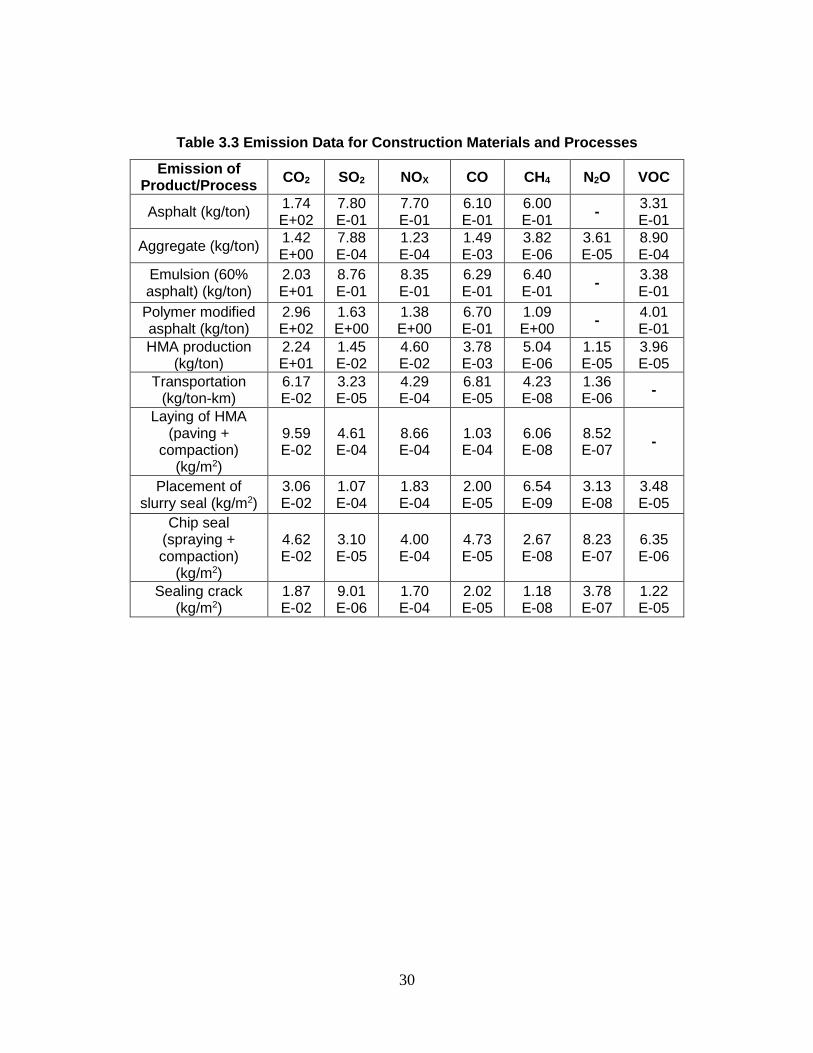
exist due to different local conditions, technologies, and system boundaries. Tables 3.2 and 3.3

list the inventory data for energy and emission, respectively for construction materials and

processes used in four preservation treatments considered in this study. Life inventory of

asphalt product was obtained from a report published by the European bitumen industry

(Eurobitume, 2012) that covers extraction of crude oil, manufacturing of bitumen or emulsion,

storage, and construction of production facility. A report published by the Swedish

Environmental Research Institute (IVL) (Stripple, 2001) was used to get energy consumption

and emission data for aggregate production, manufacturing of HMA, transportation, and

machinery used in construction. The life cycle inventory of crushed aggregates was based on

the production of crushed aggregates including rock blasting, stone breaking, crushing and

screening. Oil and natural gas are the greatest sources of energy consumption as they are used

during the production of raw materials.

Hot-mix asphalt thin overlay was constructed by using an asphalt paver which evenly

distributes the asphalt and aggregate mixture on the pavement surface. Asphalt was added by

a material transfer unit into the paver’s hopper. A conveyor then carries the asphalt from hopper

to auger after which the auger places a stockpile of material in front of the screed and then the

screed spreads the material over the width of the road and gives initial compaction. A very

important task of the paver is to provide a smooth uniform surface behind the screed. For this

task a screen is provided to smooth the surface. The screen is a free floating type device

attached at the end. The height of the screen can be managed and so can the effect of it. In this

study the asphalt paver used is the model Dynapac F16 from Dynapac. The final step in

construction of the thin overlay was compaction of the layer using a Dynapac 142 CC asphalt

compactor. The engine data has been taken from model data presented in the Stripple (2011)

inventory data report. Calculations were according to Dynapac’s product program. Laying speed

was assumed constant at 4 m/min. The width of the screen can be varied according to the

project’s requirement. For Dynapac F16, the fuel consumption is 22 liter/ hour and the paving

speed is 240 m/h.

The slurry seal is made with a consistency that can be spread over the pavement by

using a spreader box. The surface is wetted before spreading the slurry which makes a better

bonding between the pavement and the slurry seal material. In this study, type II slurry seal was

used with a thickness of 0.25 inches. Slurry seal should not be applied during nighttime and rain

28

because water evaporation is very important for the final strength of the slurry seal surface.

Emulsified asphalt, water and aggregate were mixed in a mixer. The sequence of adding is as

follows: aggregate, water, additives and then emulsion. The mixer shall be capable of mixing

ingredients together in a proper consistency and should prevent foaming. The spreader is

attached to the surface of the slurry mixing unit. Slurry was introduced into the spreader box

which lays down the slurry coating onto the surface (International slurry surfacing association).

The slurry seal machine used for construction was a Bergkamp M206, it is a diesel driven

machine and specifications are used mentioned in Guistizzo (2010).

In crack seal, the first step is to clean the cracks on the pavement. Sealant was made up

of emulsion based asphalt. In this study, polymer modified bitumen was considered as the

sealant for the crack seal preservation method. Laying sealant can be manual using a hose

pipe. In this study a diesel driven machine, which is used for sawing and sealing joints in

concrete road construction, An application rate of 0.37 kg/m with a crack density of 0.37 m/km

was considered for this study. A Skanska sealing machine, which operates on diesel fuel, was

used for this process. Diesel consumption for this sealing machine is 0.141 liter/m2.

Chip seals were constructed by laying a layer of asphalt emulsion or bitumen evenly and

then distributing a layer of aggregates over it. The asphalt emulsion was spread over the

pavement surface and then aggregate was laid. Asphalt emulsion was spread using an asphalt

spreader of type HM 10HD. Layer was compacted using the asphalt compactor, Dynapac 142

CC. The asphalt spreader HM 10HD consumes 3 liter/hour with an energy consumption of

3.44E-03 MJ/m2 and laying speed of 7.65 Km/h with a laying capacity of 30600 m2/h. The

compactor’s working weight is 3.6 tonnes, fuel consumption is 6.7 liter/ hour and roller width is

1.3 meter.

The transportation of the materials to the construction site was assumed to be done by a

distribution truck with a max load of 14-ton. It was assumed that the travel would include a

100% full front haul and an empty backhaul. Diesel oil is used as fuel in all of the equipment

used for construction and transportation.

29

Table 3.2 Energy Data for Construction Materials and Processes

Energy of Product/Process

Natural gas

Oil Hydro power

Electricity Coal Total

Asphalt (J/ton) 8.65 E+08

2.17 E+09

- - 4.10 E+07

3.08 E+09

Aggregate (J/ton) - 2.10 E+07

1.00 E+07

- 1.00 E+06

3.20 E+07

Emulsion (60% asphalt) (J/ton)

9.42 E+08

1.93 E+09

- - 2.13 E+08

3.09 E+09

Polymer modified asphalt (J/ton)

2.25 E+09

2.97 E+09

- - 7.20 E+08

5.94 E+09

HMA production (J/ton)

3.40 E+05

2.85 E+08

4.60 E+07

3.60 E+07

1.40 E+06

3.69 E+08

Transportation (J/ton-km)

- 9.01 E+05

- - - 2.90 E+07

Laying of HMA (paving +

compaction) (J/m2) -

1.30 E+06

- - - 1.30 E+06

Placement of slurry seal (J/m2)

- 4.20 E+05

- - - 4.20 E+05

Chip seal (spraying +

compaction) (J/m2) -

6.00 E+05

- - - 6.00 E+05

30

Table 3.3 Emission Data for Construction Materials and Processes

Emission of Product/Process

CO2 SO2 NOX CO CH4 N2O VOC

Asphalt (kg/ton) 1.74 E+02

7.80 E-01

7.70 E-01

6.10 E-01

6.00 E-01

- 3.31 E-01

Aggregate (kg/ton) 1.42 E+00

7.88 E-04

1.23 E-04

1.49 E-03

3.82 E-06

3.61 E-05

8.90 E-04

Emulsion (60% asphalt) (kg/ton)

2.03 E+01

8.76 E-01

8.35 E-01

6.29 E-01

6.40 E-01

- 3.38 E-01

Polymer modified asphalt (kg/ton)

2.96 E+02

1.63 E+00

1.38 E+00

6.70 E-01

1.09 E+00

- 4.01 E-01

HMA production (kg/ton)

2.24 E+01

1.45 E-02

4.60 E-02

3.78 E-03

5.04 E-06

1.15 E-05

3.96 E-05

Transportation (kg/ton-km)

6.17 E-02

3.23 E-05

4.29 E-04

6.81 E-05

4.23 E-08

1.36 E-06

-

Laying of HMA (paving +

compaction) (kg/m2)

9.59 E-02

4.61 E-04

8.66 E-04

1.03 E-04

6.06 E-08

8.52 E-07

-

Placement of slurry seal (kg/m2)

3.06 E-02

1.07 E-04

1.83 E-04

2.00 E-05

6.54 E-09

3.13 E-08

3.48 E-05

Chip seal (spraying + compaction)

(kg/m2)

4.62 E-02

3.10 E-05

4.00 E-04

4.73 E-05

2.67 E-08

8.23 E-07

6.35 E-06

Sealing crack (kg/m2)

1.87 E-02

9.01 E-06

1.70 E-04

2.02 E-05

1.18 E-08

3.78 E-07

1.22 E-05

31

3.3 Energy and Emission of Different Preservation Treatments

Tables 3.4, 3.5, 3.6 and 3.7 show the calculated energy use and emissions at the construction

stage for one lane-mile of surface area, respectively, for thin overlay, slurry seal, chip seal and

crack seal. The energy consumption was summed up with the break-up of energy resources

such as natural gas, oil, electricity, and coal fuel. The emission values were calculated for

carbon dioxide (CO2), sulfur oxide (SOx), nitrogen oxide (NOx), carbon monoxide (CO), nitrous

oxide (N2O), methane (CH4), and volatile organic component (VOC).

Table 3.4 shows energy and emissions for hot mix asphalt thin overlay with 1.5 inch

thickness and the proportion of asphalt and aggregate is 5% and 95% respectively. Table 3.5

shows energy and emissions for the type II slurry seal made of emulsion 14% and aggregate

86%, with an application rate of 1.218 kg/m2 and 7.482 kg/m2 for emulsion and aggregate

respectively. Table 3.6 shows energy and emissions for chip seal with an application rate of

1.632 kg/m2 and 15 kg/m2 respectively. Table 3.7 shows energy and emissions for energy and

emissions for crack seal using polymer modified bitumen with an application rate of 0.37 kg/m2

and crack density of 0.37 m/m2.

Table 3.4 Energy Consumption and Emission for One Lane-Mile HMA Overlay

Process Raw Material

Manufacture Transport

Placement Total Asphalt Aggregate (20 mile)

Amount (ton)

26 492 518 518

Energy (J)

Natural Gas 2.25E+10 - 1.76E+08 - - 2.27E+10

Oil 5.65E+10 1.03E+10 1.48E+11 1.50E+10 7.49E+09 5.22E+11

Hydropower energy

- - 2.38E+10 - - 2.87E+10

Electricity - - 1.86E+10 - - 1.86E+10

Fuel 1.07E+09 4.92E+08 7.25E+08 - - 2.28E+09

Total 8.00E+10 1.57E+10 1.91E+11 1.50E+10 7.49E+09 5.95E+11

Emissions to Air (kg)

SOx 1.03E+00 1.97E+01 7.54E+00 5.39E-01 2.67E-01 2.90E+01

NOx 1.00E+00 1.91E+01 1.97E+00 7.16E+00 5.02E+00 3.42E+01

CO2 2.61E+02 4.97E+03 1.16E+04 1.12E+03 5.56E+02 1.85E+04

CO 8.34E-01 1.58E+01 1.97E+00 1.14E+00 5.99E-01 2.04E+01

N2O - - 5.98E-03 2.27E-02 4.94E-03 3.36E-02

CH4 1.47E+01 2.79E+02 2.62E-03 7.10E-04 3.51E-04 2.94E+02

VOC 8.18E+00 1.55E+02 2.06E-02 - - 1.64E+02

32

Table 3.5 Energy Consumption and Emission for One Lane-Mile Slurry Seal

Process Material

Transport Placement Total Emulsion Aggregate

Amount (ton)

11 67 78

Energy (J)

Natural Gas 1.04E+10 1.32E+07 - - 1.04E+10

Oil 2.12E+10 1.41E+09 2.26E+09 2.42E+09 7.03E+10

Hydropower energy

- 6.67E+08 - - 6.67E+08

Electricity - - - - -

Fuel 2.33E+09 6.33E+07 0.00E+00 0.00E+00 2.40E+09

Total 3.39E+10 2.15E+09 2.26E+09 2.42E+09 8.37E+10

Emissions to Air (kg)

SOx 8.71E-01 5.35E+00 5.22E-02 6.19E-01 6.89E+00

NOx 8.26E-01 5.07E+00 6.94E-01 1.06E+00 7.65E+00

CO2 2.10E+02 1.29E+03 1.09E+02 1.77E+02 1.79E+03

CO 6.31E-01 3.87E+00 1.54E+00 1.16E-01 6.16E+00

N2O 2.19E-04 1.35E-03 5.50E-03 1.82E-04 7.25E-03

CH4 6.33E-01 3.89E+00 6.88E-05 3.79E-05 4.52E+00

VOC 3.39E-01 2.09E+00 - 2.02E-01 2.63E+00

Table 3.6 Energy Consumption and Emission for One Lane-Mile Chip Seal

Process Material Transport

(20 mile) Placement Total

Emulsion Aggregate

Amount (ton)

10 87 97

Energy (J)

Natural Gas 9.42E+09 1.71E+07 - - 9.44E+09

Oil 1.93E+10 1.83E+09 2.82E+09 3.46E+09 8.09E+10

Hydropower energy

- 8.67E+08 - - 8.67E+08

Electricity - - - - -

Fuel 2.13E+09 8.20E+07 - - 2.21E+09

Total 3.09E+10 2.79E+09 2.82E+09 3.46E+09 9.34E+10

Emissions to Air (kg)

SOx 8.29E+00 6.85E-02 9.98E-02 1.80E-01 8.63E+00

NOx 7.90E+00 1.07E-02 1.33E+00 2.32E+00 1.16E+01

CO2 1.92E+03 1.23E+02 2.08E+02 2.68E+02 2.52E+03

CO 5.95E+00 1.30E-01 2.95E+00 2.74E-01 9.30E+00

N2O 0.00E+00 3.14E-03 4.21E-03 4.77E-03 1.21E-02

CH4 6.05E+00 3.32E-04 1.32E-04 1.55E-04 6.05E+00

33

VOC 3.20E+00 7.74E-02 - 3.78E-02 3.31E+00

Table 3.7 Energy Consumption and Emission for One Lane-Mile Crack Seal

Process Material –

sealant (ton) Transport (20 mile)

Placement Total

Amount (ton) 1 16

Energy (J)

Natural Gas 2.25E+09 - - 1.79E+09

Oil 2.97E+09 4.57E+08 7.50E+07 4.93E+09

Hydropower energy

- - - -

Electricity - - - -

Fuel 7.20E+08 - - 5.71E+08

Total 5.94E+09 4.57E+08 7.50E+07 5.71E+08

Emissions to Air (kg)

SOx 1.31E+00 8.22E-04 5.22E-02 1.36E+00

NOx 1.11E+00 1.09E-02 9.80E-01 2.10E+00

CO2 2.38E+02 1.71E+00 1.08E+02 3.48E+02

CO 5.40E-01 2.43E-02 1.17E-01 6.81E-01

N2O - 3.46E-05 2.19E-03 2.23E-03

CH4 8.73E-01 1.08E-06 6.86E-05 8.73E-01

VOC 3.23E-01 - 7.05E-02 3.93E-01

3.4 Summary

In this chapter the inventory analysis and the impact assessment were conducted for the

construction stage of pavement preservation. Energy consumption and different emissions were

quantified for construction of thin overlay, slurry seal, crack seal and chip seal using life

inventory data obtained from the previous studies. The construction stage analysis contains

energy consumption and GHG emissions at material, manufacture, transportation and

placement phases.

34

Chapter 4 EMISSION AND ENERGY AT USAGE STAGE OF PAVEMENT

4.1 MOVES (Motor Vehicle Emission Simulator) Overview

MOVES2010b is the highway vehicle emissions model developed by the U.S. Environmental

Protection Agency (EPA). It calculates on-road emissions of all on-road vehicles including

motorcycles, cars, different trucks and buses on different types of roads such as - rural

restricted access, rural unrestricted access, urban restricted access and urban unrestricted

access. It calculates various emissions like running exhaust, start exhaust, various evaporative

emissions, tire wear and break wear. The classification system of the Federal Highway

Administration’s Highway Performance Monitoring System (HPMS) was used in MOVES.

MOVES can be used in different geographic scales such as national, county, state or

multi state level. The user provides information related to the project like specific geographical

area, vehicle type, road type, and time frame. It performs series of calculations to estimate

emissions and energy consumption based on the user input and default information present in

the model. It factors in Vehicle Specific Power (VSP), Vehicles Miles Travelled (VMT), rolling

resistance coefficient, rolling factors, drag force, fixed mass factors, and vehicle age distribution.

One of the important factors in calculating the energy consumption and GHG emission is the

condition of the vehicle, which is called the operating mode i.e. start, idle, running. For

determining a specific emissions profile, a run specification is prepared defining place, time,

vehicle, road, fuel type, GHG emission, producing process and pollutant parameters

(MOVES2010b user guide, 2012).

The MOVES model considers various parameters like speed, grade, roughness, texture

depth, traffic volume, engine running status and analyzes them together to get the output. The

power of the vehicle has an impact on the fuel consumption, which eventually impacts the

emissions and energy consumption. The Vehicle Specific Power (VSP) factors in the running

status of the engine for unit vehicle at various speeds. It has various operating modes that

represent the various stages of the vehicle operating mode like acceleration, braking, idling,

speed coasting, soaking time, tire-wear, break-wear as well as the various speeds. With

changing conditions of the vehicle from start to acceleration or from deceleration and eventual

stop, the power demand changes. This change is measured in MOVES with the operating

modes defined in the VSP data. The vehicle’s engine needs power to overcome the

35

aerodynamic drag, rolling resistance, friction, engine’s drag, and gradient forces. VSP connects

the effects of the rolling resistance to the energy consumption and emissions.

4.2 Consideration of Road Surface Characteristics in MOVES

As discussed previously, MOVES uses vehicle specific power (VSP) as one of the important

factors to calculate the engine running status. VSP is the factor that distinguishes between

running activity modes.

MOVES works by calculating the speed of the vehicle second by second to calculate various

emissions. The relationship between VSP and factors associated with the vehicle is shown in

Equation (4.1).

VSP = (A/M) * ν + (B/M) * ν2 + (C/M) * ν3 + (α+g *sinθ) * ν ……………… (4.1)

Where, A, B, and C are coefficients in kW·s/m, kW·s2/m2 and kW·s3/m3, respectively;

A coefficient represents the rolling resistance component;

B describes higher order rolling resistance factor in addition to mechanical rotating

friction losses;

C coefficient represents the air drag coefficient component;

M is the fixed mass factor in metric tons;

g is the acceleration due to gravity (9.8 m/s2);

ν is the vehicle speed in meter/second;

α is the vehicle acceleration in meter/second2; and

sin θ is the (fractional) road grade.

Default values of A, B and C are derived from track load horsepower from Mobile source

observation database (MSOD) (U.S.EPA, 2010a). These values are obtained by dynamometer

tests of the vehicles.

The Highway Development and Management (HDM-4) model is a tool developed by

PIARC (World Road Association) to perform a cost analysis for maintenance and rehabilitation

of roads. It also has a model with rolling resistance based on IRI and MPD and was calibrated to

North American vehicles by Zaabar and Chatti (2010). This model also takes account of the

effects of rolling resistance caused by pavement deflection. The HDM-4 model is unable to

consider speed variations and works only with the steady speed of vehicles, which is unrealistic

in real driving conditions. In this study, equations 4.2, 4.3 and 4.4 by the HDM-4 model were

used to calculate rolling resistance and then the MOVES model was used to calculate the fuel

consumption and emissions.

In the HDM-4 model rolling resistance is calculated using equations (4.2) and (4.3)

36

Fr = CR2 x FCLIM x [b11 x Nw + CR1(b12 x M + b13 x v2)] …….. (4.2)

CR2 = Kcr2 x (a0 + a1 x MTD + a2 x IRI + a3 x DEF) …………..... (4.3)

Where, Fr is the rolling resistance;

CR1 is the function of tire type;

CR2 is the factor of surface characteristics;

FCLIM is the climatic factor related to the percentage of driving snow and rain;

b1, b12, and b13 are the coefficients related to tire type and other technologies;

Kcr2 is a calibration factor;

a0, a1, a2 and a3 are coefficients for pavement surface characteristics from HDM-4;

MTD is mean texture depth;

IRI is the international roughness index;

DEF is Benkelman Beam rebound deflection; M is the mass of the vehicles;

Nw is the number of wheels; and

v is the speed.

The MOVES model is equipped with an inbuilt database with lots of default data to

execute runs to calculate emissions. The MOVES model default data needs to be combined

with the other input data of the project to get emission outputs. The default data is derived from

dynamometer tests of vehicles. In this test, the vehicle is made to run on a smooth surface,

mostly steel (Wang et al. 2011). Both IRI and MPD values are zero because this surface is

much smoother than the real pavement. Thus, the contribution of pavement surface

characteristics to vehicle operation is considered by updating the rolling resistance coefficient

(A) in MOVES. The relationship between Aupdated and Adefault is shown in equation (4.4). This

relationship is established by Wang et al. (2012) in their study.

Aupdated= Adefault *(CR2pavement/CR2dynamometer) …….. (4.4)

Where, CR2 is same as Equation (4.3).

IRI and MTD were assumed to be zero for the dynamometer test in this study, while for

the passenger car DEF is also zero. By updating IRI values for different preservation cases for

both the sites in CR2pavement equation 4.3, we get the Aupdated which is further updated into

“sourceusetype” file in MOVES to calculate the emissions. This factor is combined with the

MOVES default data of the rotating friction losses. The data represents the roughness and the

traffic volume of the sites with different preservations for over 10 years. The IRI varies from 0.8

to 3.2 m km-1 for all the vehicle cases. For this study, the deflection value was assumed to be

zero for passenger cars while it is 0.3556 mm for the other two vehicle types. In this analysis,

37

the IRI and MPD values were varied for different pavement preservation treatments. Using the

HDM-4 model Aupdated was calculated. Then by changing the traffic volume and Aupdated, energy

and emissions were calculated by putting the values in MOVES for execution. The HDM-4

model was used to get rolling resistance values; the equations were based on changing the IRI,

MPD and MTD values for various types of vehicles. These updated values were used to

develop input for MOVES (U.S. EPA, 2010b). Finally traffic information for specific sections of

pavements and with roughness data for different preservation treatments were used by MOVES

to calculate the vehicle fuel consumption and GHG emissions.

Table 4.1 Parameters for CR2 model in HDM 4 Model

(Bennett and Greenwood, 2003)

Vehicle Adefault Vehicle weight

(kg)

a0 a1 a2 a3

Passenger Car 0.1565 <=2500 0.5 0.02 0.1 0

Passenger Truck 0.2212 >2500 0.57 0.04 0.04 1.34

Single Unit Haul Truck 0.5619 >2500 0.57 0.04 0.04 1.34

4.3 Pavement Factors Affecting Vehicle Emission and Energy

The surface of a pavement consists of different kinds of textures, grainy texture of fine

aggregates and micro-texture of coarse aggregate that are less than 0.5 mm in length. Macro-

texture is measured as one of the features of the pavement that approximately ranges from 0.5

mm to 50 mm in length (McGhee et al., 2003). MTD values were calculated using the traditional

sand patch method. IRI is the International roughness index which is used to measure

roughness of longitudinal road profile. IRI came into existence in 1986, since then it has become

the most commonly used evaluation and management tool for road systems. When

preservations methods are applied on any pavement, it affects the road surface characteristics.

Comparable to the application of thin overlay, it decreases the roughness significantly in the

starting days but then roughness again increases with usage. When crack seal is applied, it has

almost no effect as we just cover the cracks and not the whole surface of pavement. Chip seal

may produce a very rough texture on the road surface since fine aggregates are used to cover

the pavement surface.

Tables 4.11 and 4.12 represent energy and emissions for three vehicles at different

values of MTD. Figure 4.2 shows the percentage change in total energy and emissions (CO2),

38

respectively for passenger cars, passenger trucks and single unit haul trucks. IRI and deflection

were kept constant to perform the sensitivity analysis of total energy and GHG emissions based

on changing MTD. The IRI value is kept constant at 2 m/km and deflection is taken as 0.457

mm. The results represented in Figure 4.2 show that the energy and CO2 emission increases

from 0% to 0 .83% for passenger cars, 0% to 1.7% for passenger trucks and 0% to 1.08% for

single unit haul trucks when MTD was increased from 0.79 mm to 2.63 mm.

Table 4.2 Sensitivity Analysis of Energy Consumption at Different MTDs

MTD (mm)

Type of vehicles 1.10 1.40 1.71 2.01 2.32 2.63

Energy (J)

Passenger Car 1.58E+11 1.58E+11 1.58E+11 1.58E+11 1.58E+11 1.59E+11

Passenger Truck 2.01E+12 2.01E+12 2.02E+12 2.02E+12 2.03E+12 2.03E+12

Single Unit Haul Truck 9.31E+13 9.33E+13 9.35E+13 9.36E+13 9.37E+13 9.39E+13

Figure 4.1 Effect of MTD on Energy and Emission

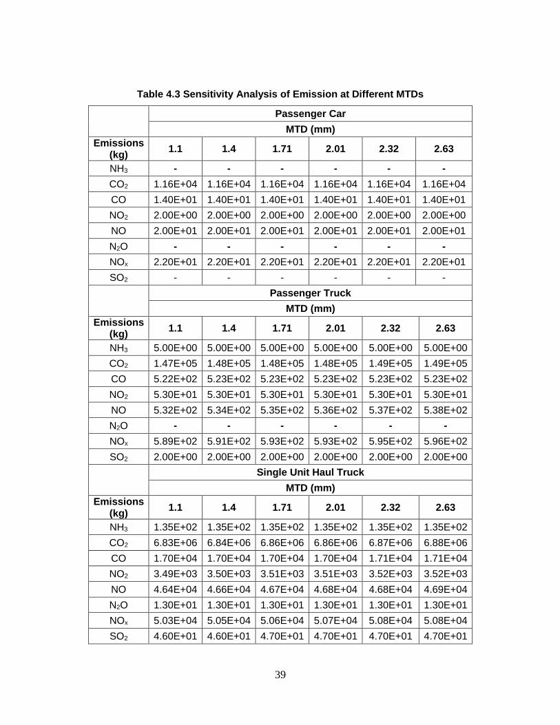
39

Table 4.3 Sensitivity Analysis of Emission at Different MTDs

Passenger Car

MTD (mm)

Emissions (kg)

1.1 1.4 1.71 2.01 2.32 2.63

NH3 - - - - - -

CO2 1.16E+04 1.16E+04 1.16E+04 1.16E+04 1.16E+04 1.16E+04

CO 1.40E+01 1.40E+01 1.40E+01 1.40E+01 1.40E+01 1.40E+01

NO2 2.00E+00 2.00E+00 2.00E+00 2.00E+00 2.00E+00 2.00E+00

NO 2.00E+01 2.00E+01 2.00E+01 2.00E+01 2.00E+01 2.00E+01

N2O - - - - - -

NOx 2.20E+01 2.20E+01 2.20E+01 2.20E+01 2.20E+01 2.20E+01

SO2 - - - - - -

Passenger Truck

MTD (mm)

Emissions (kg)

1.1 1.4 1.71 2.01 2.32 2.63

NH3 5.00E+00 5.00E+00 5.00E+00 5.00E+00 5.00E+00 5.00E+00

CO2 1.47E+05 1.48E+05 1.48E+05 1.48E+05 1.49E+05 1.49E+05

CO 5.22E+02 5.23E+02 5.23E+02 5.23E+02 5.23E+02 5.23E+02

NO2 5.30E+01 5.30E+01 5.30E+01 5.30E+01 5.30E+01 5.30E+01

NO 5.32E+02 5.34E+02 5.35E+02 5.36E+02 5.37E+02 5.38E+02

N2O - - - - - -

NOx 5.89E+02 5.91E+02 5.93E+02 5.93E+02 5.95E+02 5.96E+02

SO2 2.00E+00 2.00E+00 2.00E+00 2.00E+00 2.00E+00 2.00E+00

Single Unit Haul Truck

MTD (mm)

Emissions (kg)

1.1 1.4 1.71 2.01 2.32 2.63

NH3 1.35E+02 1.35E+02 1.35E+02 1.35E+02 1.35E+02 1.35E+02

CO2 6.83E+06 6.84E+06 6.86E+06 6.86E+06 6.87E+06 6.88E+06

CO 1.70E+04 1.70E+04 1.70E+04 1.70E+04 1.71E+04 1.71E+04

NO2 3.49E+03 3.50E+03 3.51E+03 3.51E+03 3.52E+03 3.52E+03

NO 4.64E+04 4.66E+04 4.67E+04 4.68E+04 4.68E+04 4.69E+04

N2O 1.30E+01 1.30E+01 1.30E+01 1.30E+01 1.30E+01 1.30E+01

NOx 5.03E+04 5.05E+04 5.06E+04 5.07E+04 5.08E+04 5.08E+04

SO2 4.60E+01 4.60E+01 4.70E+01 4.70E+01 4.70E+01 4.70E+01

40

The IRI is the International Roughness Index, which is used for measuring the

roughness of longitudinal road profile. The IRI’s value range of 0.8 to 3.2 m/km was used for

calculations in this study. Tables 4.13 and 4.14 represent values for total energy and emissions

for passenger car, passenger truck and single unit haul truck, for different IRI values of

pavement.

Figure 4.3 shows the percentage change of total energy change and GHG emission,

respectively for passenger cars, passenger trucks and single unit haul trucks. MTD and

deflection were kept constant at 1.4 mm and 0.203 mm to perform the sensitivity analysis of the

total energy and GHG emission based on changing the IRI. The results represented in Figure

4.3 show that the energy and CO2 emission increased from 0% to 5.65% for passenger cars,

0% to 2.1 % for passenger trucks and 0% to 1.72% for single unit haul trucks when the IRI was

increased from 0.8 m/km to 3.2 m/km.

Table 4.4 Sensitivity Analysis of Energy Consumption at Different IRIs

IRI (m/km)

Type of vehicles 0.8 1.4 2 2.6 3.2

Energy (J)

Passenger Car 1.53E+11 1.56E+11 1.58E+11 1.60E+11 1.65E+11

Passenger truck 1.86E+12 1.87E+12 1.87E+12 1.89E+12 1.90E+12

Single Unit Haul Truck

8.76E+13 8.81E+13 8.84E+13 8.87E+13 8.91E+13

Figure 4.2 Effect of IRI on Energy and Emission

41

Table 4.5 Sensitivity Analysis of Emission at Different IRIs

Passenger Car

IRI (m/km)

Emissions (kg)

0.8 1.4 2 2.6 3.2

NH3 - - - - -

CO2 1.13E+04 1.14E+04 1.16E+04 1.18E+04 1.19E+04

CO 1.40E+01 1.40E+01 1.40E+01 1.50E+01 1.50E+01

NO2 2.00E+00 2.00E+00 2.00E+00 2.00E+00 2.00E+00

NO 1.90E+01 2.00E+01 2.00E+01 2.00E+01 2.10E+01

N2O - - - - -

NOx 2.10E+01 2.20E+01 2.20E+01 2.20E+01 2.20E+01

SO2 - - - - -

Passenger Truck

IRI (m/km)

Emissions (kg)

0.8 1.4 2 2.6 3.2

NH3 5.00E+00 5.00E+00 5.00E+00 5.00E+00 5.00E+00

CO2 1.36E+05 1.37E+05 1.37E+05 1.38E+05 1.39E+05

CO 5.13E+02 5.14E+02 5.14E+02 5.14E+02 5.15E+02

NO2 4.90E+01 4.90E+01 4.90E+01 4.90E+01 5.00E+01

NO 3.28E+02 3.30E+02 3.31E+02 3.33E+02 3.35E+02

N2O - - - - -

NOx 3.64E+02 3.66E+02 3.67E+02 3.69E+02 3.71E+02

SO2 1.00E+00 1.00E+00 1.00E+00 1.00E+00 1.00E+00

Single Unit Haul Truck

IRI (m/km)

Emissions (kg)

0.8 1.4 2 2.6 3.2

NH3 1.35E+02 1.35E+02 1.35E+02 1.35E+02 1.35E+02

CO2 6.42E+06 6.46E+06 6.48E+06 6.50E+06 6.53E+06

CO 1.67E+04 1.67E+04 1.68E+04 1.68E+04 1.68E+04

NO2 3.25E+03 3.27E+03 3.29E+03 3.30E+03 3.32E+03

NO 4.31E+04 4.34E+04 4.36E+04 4.38E+04 4.40E+04

N2O 1.30E+01 1.30E+01 1.30E+01 1.30E+01 1.30E+01

NOx 4.68E+04 4.71E+04 4.73E+04 4.75E+04 4.77E+04

SO2 4.40E+01 4.40E+01 4.40E+01 4.40E+01 4.40E+01

42

Every time a vehicle moves over a pavement, its wheels put load on the underneath

surface and it results in a deflection on the pavement surface. A single vehicle only causes a

very small deformation of the pavement but when it is combined for a large amount of vehicle

traffic, it plays an important role while considering the contribution of pavement surface

deflection to the tire rolling resistance.

The deflection range used in this analysis was 8 mils (0.2032 mm), 14 mils (0.3556 mm),

18 mils (0.4572 mm) and 20 mils (0.5080 mm). IRI was 2 m/km and MTD was 1.4 mm with

varying deflection values. Tables 4.15 and 4.16 represent energy and emissions for three

vehicles at different values of deflections. The results represented in Figure 4.4 show that the

energy and CO2 emissions increased from 0% to 8.8 % for passenger trucks and 0% to 6.67%

for single unit haul trucks when deflection was increased from 0.2032 mm to 0.5080 mm. The

effect of deflection on the tire rolling resistance was neglected for passenger cars because the

value of a3 is zero in CR2 (Equation 4.4).

Table 4.6 Sensitivity Analysis of Energy Consumption at Different Deflections

Deflection (mm)

Type of vehicles 0.2032 0.3556 0.4572 0.5080

Energy (J)

Passenger Car - - - -

Passenger truck 1.87 E+12

1.96 E+12

2.01 E+12

2.04 E+12

Single Unit Haul Truck 8.84 E+13

9.12 E+13

9.33 E+13

9.44 E+13

Figure 4.3 Effect of Deflection on Energy and Emission

43

Table 4.7 Sensitivity Analysis of Emission at Different Deflections

Deflection (mm)

0.2032 0.3556 0.4572 0.508

Emissions (kg)

Passenger Truck

NH3 5.00 E+00

5.00 E+00

5.00 E+00

5.00 E+00

CO2 1.37 E+05

1.44 E+05

1.48 E+05

1.49 E+05

CO 5.14 E+02

5.19 E+02

5.23 E+02

5.24 E+02

NO2 4.90 E+01

5.10 E+01

5.30 E+01

5.30 E+01

NO 4.97 E+02

5.18 E+02

5.34 E+02

5.40 E+02

NOx 5.50 E+02

5.74 E+02

5.91 E+02

5.98 E+02

SO2 1.00 E+00

1.00 E+00

1.00 E+00

1.00 E+00

Emissions (kg)

Single Unit Haul Truck

NH3 1.35 E+02

1.35 E+02

1.35 E+02

1.35 E+02

CO2 6.48 E+06

6.69 E+06

6.84 E+06

6.92 E+06

CO 1.68 E+04

1.69 E+04

1.70 E+04

1.71 E+04

NO2 3.29 E+03

3.41 E+03

3.50 E+03

3.54 E+03

NO 4.36 E+04

4.53 E+04

4.66 E+04

4.72 E+04

N2O 1.30 E+01

1.30 E+01

1.30 E+01

1.30 E+01

NOx 4.73 E+04

4.91 E+04

5.05 E+04

5.12 E+04

SO2 4.40 E+01

4.50 E+01

4.60 E+01

4.70 E+01

4.4 Summary

The HDM-4 and MOVES 2010 EPA model were used to analyze the sensitivity of vehicle

emissions and fuel/energy consumption affected by different factors. The HDM-4 model was

used to calculate the changes in tire rolling coefficients due to pavement surface characteristics

and then different rolling resistance coefficients were used in MOVES. Road surface factors like

MTD, IRI and deflection were used to evaluate their effects on vehicle emissions and energy

consumption.

44

Chapter 5 LIFE-CYCLE ENERGY AND EMISSIONS OF PAVEMENT PRESERVATION

5.1 Effect of Preservation on Pavement Roughness

It is expected that the pavement preservation could improve pavement surface smoothness. Lu

and Tolliver (2012) performed a study and designed an optimization model based on the Pareto

optimal concept to solve all types of constraints to minimize costs and maximize benefits. They

studied short-term effectiveness in the IRI change, using long term pavement program data and

found that the pavement treatment short-term effectiveness in IRI follows a polynomial

relationship with pre-treatment condition. They observed average reductions of 1.44 m/km IRI

for hot mill overlay, average reduction of 0.27 m/km IRI for crack sealing and average

reductions of 0.72 m/km for chip seal.

Wang et al. (2012) performed a study on preservation treatments using the roughness

data from experiment sites in the long-term pavement performance program (LTPP). State

maintenance engineers were included in a survey to obtain experience of utilizing pavement

treatments. HMA overlay was found to have the highest performance time of 9 years followed

by micro-surfacing with chip seal (6 years), slurry seal (4 years), crack filling (4 years) and crack

sealing (3 years). Thin overlay was found to be the most expensive followed by micro-surfacing,

chip seal tied with slurry seal. The authors used a paired t-test to compare the roughness of the

treatment section with that of the control sections. By using a paired t-test the authors found that

all the treatments significantly reduced long term roughness of the pavement. The order of

effectiveness is as follows: HMA overlay followed by chip seal, crack seal and slurry seal. When

control section and crack sealing were compared for roughness factor, mean difference of ΔIRI

was found to be 0.124 with a standard deviation of 0.269. The mean difference of ΔIRI between

control sections and slurry sealing section is 0.083, with a standard deviation of 0.04. Finally,

the mean difference of ΔIRI between control section and overlay section is 0.407 with a

standard deviation of 0.618.

Carvalho et al. (2011) studied impacts of design features in pavement response and

performance in rehabilitated flexible and rigid pavements. They used a performance indicator

named weighted distress, which represents the total normalized area (per year) under the

distress versus time curve. Particular site sections were surveyed for 8 years for IRI values. All

the sections were observed with a similar IRI for the experiment. In the analysis period, thin

overlay performed better than other treatments with a Weighted Distress-IRI (WD-IRI) value of

45

4.80 Ft/mi (0.91 m/km) while slurry seal was found to have a WD-IRI value of 7.66 ft/mi (1.45

m/km) and shows the worst performance over an 8 year time period.

In this study, pavement roughness data was collected from the specific pavement

studies (SPS) of the long-term pavement performance program (LTPP). Two sites were

selected from LTPP-SPS3 where preservation treatments were applied once during the whole

period for the study. Each site was provided with four preservation treatments – thin overlay,

slurry seal, crack seal and chip seal; they are applied with average length of 500ft with an extra

control section to monitor the difference and effects. Figures 5.1 and 5.2 represent roughness

values from the LTPP-SPS3 project for two sites, site 17 and site 27, for different preservation

and control sections used in this study. The effect of pavement preservation on surface

roughness is more significant at site 27 because it has the greater initial roughness.

Figure 5.1 Roughness data at Site 17 from LTPP- SPS3

46

Figure 5.2 Roughness Data at Site 27 from LTPP- SPS3

For the emission and energy analysis in this study, the MTD was assumed to be 1.4 mm

and the deflection value was assumed to be 0.3556 mm for the whole analysis.

5.2 Effect of Pavement Preservation on Energy and Emissions at Usage Stage

Table 5.1 shows the total energy consumption obtained by running input data on MOVES for

site 17 and site 27 with an annual traffic volume of 10 million, respectively for the different

preservation treatments along with the control section. Energy consumption is in Joules for all

the vehicles and the preservation treatment types. The traffic percentage considered was 45%-

45% each for the passenger cars and the passenger trucks and 10% for the single unit haul

trucks. Table 5.2 shows the total energy for both sites considering the truck percentage for the

traffic.

Table 5.1 Energy Consumption in MJ during Usage Stage

(10 Million Annual Traffic Volume)

Energy (J) Control Chip seal

Crack seal

Slurry seal

Thin overlay

Passenger Car

Site 17 2.1772 E+12

2.1739 E+12

2.1742 E+12

2.1733 E+12

2.1613 E+12

Site 27 1.1312 E+12

1.1193 E+12

1.1157 E+12

1.1159 E+12

1.0785 E+12

Passenger Truck

Site 17 2.7293 E+13

2.7272 E+13

2.7274 E+13

2.7268 E+13

2.7498 E+13

Site 27 1.3715 1.3661 1.365 1.3648 1.3484

47

E+13 E+13 2E+13 E+13 E+13

Single Unit Haul Truck

Site 17 1.2756 E+15

1.2752 E+15

1.2752 E+15

1.2753 E+15

1.2717 E+15

Site 27 6.3764 E+14

6.3560 E+14

6.3512 E+14

6.3504 E+14

6.2983 E+14

Table 5.2 Energy Consumption Using Truck Percentage during Usage Stage

Energy (J)

Control Chip seal

Crack seal

Slurry seal

Thin overlay

Site 17 1.4082 E+14

1.4077 E+14

1.4078 E+14

1.4078 E+14

1.4052 E+14

Site 27 7.0445 E+13

7.0211 E+13

7.0157 E+13

7.0148 E+13

6.9536 E+13

Table 5.3 shows the emission for both sites 17 and 27 with the truck percentage

mentioned for different preservation treatments and the control section. For both sites the

highest amount of CO2 was observed for control section and the lowest was observed for thin

overlay. N2O and SO2 emissions were same for all the preservation treatments.

Table 5.3 Emission Values with Truck Percentage during Usage Stage

Site 17

Emissions (kg)

CO2 CO NO2 NO NOx NH3 N2O SO2

Control 1.033 E+07

2.707 E+04

5.097 E+03

6.669 E+04

7.236 E+04

2.21 E+02

3.1 E+01

6.9 E+01

Chip seal 1.032 E+07

2.706 E+04

5.095 E+03

6.663 E+04

7.233 E+04

2.21 E+02

3.1 E+01

6.9 E+01

Crack seal 1.032 E+07

2.706 E+04

5.096 E+03

6.667 E+04

7.234 E+04

2.21 E+02

3.1 E+01

6.9 E+01

Slurry seal

1.032 E+07

2.706 E+04

5.096 E+03

6.667 E+04

7.234 E+04

2.21 E+02

3.1 E+01

6.9 E+01

Thin overlay

1.029 E+07

2.705 E+04

5.081 E+03

6.645 E+04

7.210 E+04

2.21 E+02

3.1 E+01

6.9 E+01

Site 27

CO2 CO NO2 NO NOx NH3 N2O SO2

Control 5.166 E+06

1.342 E+04

2.553 E+03

3.342 E+04

3.627 E+04

1.09 E+02

1.5 E+01

3.5 E+01

Chip seal 5.152 E+06

1.341 E+04

2.543 E+03

3.329 E+04

3.613 E+04

1.09 E+02

1.5 E+01

3.5 E+01

Crack seal 5.131 E+06

1.339 E+04

2.533 E+03

3.316 E+04

3.598 E+04

1.09 E+02

1.5 E+01

3.5 E+01

Slurry seal

5.119 E+06

1.338 E+04

2.525 E+03

3.305 E+04

3.587 E+04

1.09 E+02

1.5 E+01

3.4 E+01

48

Thin overlay

5.112 E+06

1.337 E+04

2.524 E+03

3.303 E+04

3.584 E+04

1.09 E+02

1.5 E+01

3.4 E+01

5.3 Life-Cycle Emission and Energy

After getting data for both phases, the construction and usage phase were summed up to get

the total value of energy consumption and CO2 emissions. The results in Table 5.4 are a

combination of energy consumption and emissions from the construction stage and the usage

stage for site 17. As expected, the highest amount of energy consumption and emission at the

construction stage was observed for thin overlay, while at the usage stage the highest energy

consumption and emission was observed for the control section. After adding up both stages,

the most sustainable preservation method in terms of energy was thin overlay with the lowest

energy consumption.

The reduction during the usage stage was calculated by comparing the preservation

sections to the control section. For site 17, thin overlay shows the highest energy reduction of

3.044 E+11 J, followed by chip seal, crack seal, and slurry seal. GHG emission reduction was

the highest for thin overlay 32.28 tons, followed by chip seal, crack seal, and slurry seal. The

reduction of energy consumption at the usage stage due to preservation is smaller than the

energy consumed at the construction stage, while the reduction of GHG emission at the usage

stage is much greater than the GHG emission produced at the construction stage.

The results in Table 5.5 are a combination of energy consumption and emissions from

the construction stage and the usage stage for site 27. Thin overlay shows the highest energy

reduction of 9.091E+11 J, followed by slurry seal, crack seal, and chip seal. GHG emission

reduction was highest for the thin overlay 54.14 tons, followed by slurry seal, crack seal and

chip seal. The reduction of energy consumption and GHG emission at the usage stage due to

preservation are much greater than the ones consumed at the construction stage. This

environmental benefit at the usage stage due to pavement preservation is greater at site 27

than the one at site 17 because of the effect of pavement preservation on surface roughness.

This again clearly indicates that the usage stage cannot be neglected in the LCA of pavement

and the importance of pavement surface characteristics on fuel consumption and GHG

emission.

49

Table 5.4 Change of Energy and Emission after Pavement Preservation for Site 17

Site 17 Control Thin overlay

Chip seal

Slurry seal

Crack seal

Energy (J) Construction / 5.950 E+11

9.340 E+10

8.370 E+10

5.710 E+08

Usage 1.4082 E+14

1.4052 E+14

1.4077 E+14

1.4078 E+14

1.4078 E+14

Reduction in usage

/ 3.044 E+11

5.183 E+10

4.391 E+10

4.458 E+10

CO2 (kg) Construction / 1.85 E+04

2.52 E+03

1.79 E+03

3.48 E+02

Usage 1.033 E+07

1.029 E+07

1.032 E+07

1.032 E+07

1.032 E+07

Reduction in usage

/ 3.228 E+04

3.802 E+03

3.222 E+03

3.269 E+03

CO (kg) Construction / 2.04 E+01

9.30 E+00

6.16 E+00

6.81 E-01

Usage 2.707 E+04

2.705 E+04

2.706 E+04

2.706 E+04

2.706 E+04

Reduction in usage

/ 2.300 E+01

4.142 E+00

4.000 E+00

4.000 E+00

NOx (kg) Construction / 3.423 E+01

1.16 E+01

7.655 E+00

2.10 E+00

Usage 7.236 E+04

7.210 E+04

7.233 E+04

7.234 E+04

7.234 E+04

Reduction in usage

/ 2.600 E+02

2.747 E+01

2.300 E+01

2.300 E+01

GHG (Ton) Construction / 1.887 E+01

2.650 E+00

1.880 E+00

3.700 E-01

Usage 1.034 E+04

1.030 E+04

1.033 E+04

1.033 E+04

1.033 E+04

Reduction in usage

3.228 E+01

3.802 E+00

3.222 E+00

3.269 E+00

50

Table 5.5 Change of Energy and Emission after Pavement Preservation for Site 27

Site 27 Control Thin overlay

Chip seal

Slurry seal

Crack seal

Energy (J)

Construction / 5.95 E+11

9.34 E+10

8.37 E+10

5.71 E+08

Usage 7.044 E+13

6.953 E+13

7.021 E+13

7.015 E+13

7.016 E+13

Reduction in usage

/ 9.091 E+11

2.339 E+11

2.966 E+11

2.877 E+11

CO2

(kg) Construction / 1.85

E+04 2.52 E+03

1.79 E+03

3.48 E+02

Usage 5.166 E+06

5.112 E+06

5.152 E+06

5.119 E+06

5.131 E+06

Reduction in usage

/ 5.41 E+04

1.38 E+04

4.70 E+04

3.46 E+04

CO (kg) Construction / 2.04 E+01

9.30 E+00

6.16 E+00

6.81 E-01

Usage 1.342 E+04

1.337 E+04

1.341 E+04

1.338 E+04

1.339 E+04

Reduction in usage

/ 4.400 E+01

1.232 E+01

3.800 E+01

3.100 E+01

NOx (kg)

Construction /

3.423 E+01

1.16 E+01

7.655 E+00

2.10 E+00

Usage 3.627 E+04

3.584 E+04

3.613 E+04

3.587 E+04

3.598 E+04

Reduction in usage /

4.290 E+02

1.380 E+02

4.010 E+02

2.840 E+02

GHG (Ton)

Construction / 1.887 E+01

2.650 E+00

1.880 E+00

3.700 E-01

Usage 5.171 E+03

5.116 E+03

5.157 E+03

5.124 E+03

5.136 E+03

Reduction in usage

/ 5.414 E+01

1.381 E+01

4.702 E+01

3.461 E+01

5.4 Effect of Preservation on User Costs

Fuel Consumption Costs

Fuel consumption depends on the factors affecting fuel consumption including vehicle type,

class, age, vehicle technology, pavement surface type and condition, speed, roadway geometry,

environmental condition and road grade. Factors like aerodynamic, rolling resistance, gradient,

curvature and inertial forces effect fuel consumption. Billions of dollars could be saved annually

by improving rolling resistance through maintaining pavement surface smoothness (NCHRP

report 720). Various models are available for calculating vehicle fuel consumption. These

models are also known as vehicle operating cost (VOC) models. Some of the models are the

51

Texas research and development foundation model, the World Bank’s HDM-4 model, the

Saskatchewan Canada model, the Australian road fuel consumption model, the New Zealand

VOC model, the South African VOC model and the Swedish mechanistic model for simulation

on road traffic (Chatti and Zaabar , 2012).

Among these models, the HDM-4 model is the most recent VOC model. It provides the

pavement roughness effect on fuel consumption of a vehicle (Morosiuk G., et al 2002). Zaabar

and Chatti (2010) calibrated the HDM-4 model according to the USA conditions by estimating

the increase in fuel consumption according to the pavement roughness for different vehicle

types.

In this study, the base values developed by Chatti and Zaabar (2012) in the NCHRP

report 720 were used for all the user cost calculations. The base values for user costs were

calculated for a medium car, SUV and light truck at 35 mph speed. Table 5.6 shows base

values for three vehicle types and according to the different IRI values used for calculating effect

of roughness on fuel consumption.

Table 5.6 Effect of Roughness on Fuel Consumption Cost

Vehicles

IRI (m/km)

1 2 3 4 5 6

Base value ($/mile)

Medium Car 0.089 0.092 0.094 0.096 0.098 0.102

SUV 0.100 0.102 0.106 0.108 0.109 0.113

Light Truck 0.158 0.160 0.162 0.165 0.167 0.169

Repair and Maintenance (R&M) Cost

The R&M cost includes parts and labor cost (user cost) which are required because of vehicular

wear and tear. In this study, the method proposed by Chatti and Zaabar (2012) in the NCHRP

report 720 was used to calculate the R&M cost. It gives base values in $/mile for IRI values from

1m/km to 6m/km for various vehicle types. As per the HDM-4 model, the repair and

maintenance cost is negligible for low IRI values (193 in/mile). In this study, R&M’s NPV values

for all preservation treatments are the same and positive which implies that it is expected to

produce more income than what could be gained by earning the discount rate, which shows that

the project is profitable. Table 5.7 shows base values for three vehicle types according to the

base IRI values used for calculating the effect of roughness on repair and maintenance cost.

52

Table 5.7 Effect of Roughness on Repair and Maintenance Cost

Vehicles

IRI (m/km)

1 2 3 4 5 6

Base value ($/mile)

Medium Car

0.0021 0.00212 0.00212 0.00214 0.00214 0.00216

SUV 0.0017 0.00172 0.00173 0.00175 0.00177 0.00179

Light Truck 0.0020 0.00202 0.00204 0.00206 0.00208 0.00210

Tire Cost

The HDM-4 model was calibrated according to the cars and truck for U.S. conditions by Chatti

and Zaabar (2012). The study done by Haugodegard et al. (1994) proved that there is an

increasing trend of tire wear with pavement roughness. In this study, the net present value for all

IRI values for the tire wear cost of all preservation treatments are positive which imply that the

project is profitable. Table 5.8 shows base values according to IRI values that were used for

calculating the effect of roughness on tire wear costs.

Table 5.8 Effect of Roughness on Tire Wear Costs

Vehicles IRI (m/km)

1 2 3 4 5 6

Base value ($/mile)

Medium Car 0.024 0.024 0.024 0.0264 0.0336 0.0408

SUV 0.032 0.032 0.032 0.0384 0.0544 0.0736

Light Truck 0.034 0.034 0.034 0.0408 0.0578 0.0748

Tables 5.9 and 5.10 represent values for fuel cost, repair and maintenance cost, tire cost

for different pavement sections using the pavement roughness data at site 27 and site 17,

respectively. Tables 5.11 and 5.12 represent total cost savings by preservation treatments at

the usage stage for site 27 and site 17, respectively. The user cost was calculated using the

roughness data every year after pavement preservation and then converted to the net present

value at the year of construction.

Net present value (NPV) is defined as the difference between the present value of the

cash inflows and the present value of cash outflows. Net present value measures the total

amount of gain or loss a project will produce compared to the amount that could be earned

simply by saving the money in a bank or investing it in some other opportunity that generates a

return equal to the discount rate. The discount rate is the rate of return which could be earned in

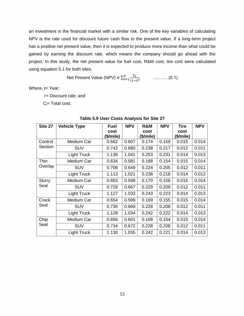
53

an investment in the financial market with a similar risk. One of the key variables of calculating

NPV is the rate used for discount future cash flow to the present value. If a long-term project

has a positive net present value, then it is expected to produce more income than what could be

gained by earning the discount rate, which means the company should go ahead with the

project. In this study, the net present value for fuel cost, R&M cost, tire cost were calculated

using equation 5.1 for both sites.

Net Present Value (NPV) = ………. (5.1)

Where, t= Year;

r= Discount rate; and

Ct= Total cost;

Table 5.9 User Costs Analysis for Site 27

Site 27 Vehicle Type Fuel cost

($/mile)

NPV R&M cost

($/mile)

NPV Tire cost

($/mile)

NPV

Control Section

Medium Car 0.662 0.607 0.174 0.159 0.015 0.014

SUV 0.742 0.680 0.238 0.217 0.012 0.011

Light Truck 1.136 1.041 0.253 0.231 0.014 0.013

Thin Overlay

Medium Car 0.634 0.581 0.168 0.154 0.015 0.014

SUV 0.708 0.649 0.224 0.205 0.012 0.011

Light Truck 1.113 1.021 0.238 0.218 0.014 0.013

Slurry Seal

Medium Car 0.653 0.598 0.170 0.156 0.015 0.014

SUV 0.728 0.667 0.229 0.209 0.012 0.011

Light Truck 1.127 1.033 0.243 0.223 0.014 0.013

Crack Seal

Medium Car 0.654 0.599 0.169 0.155 0.015 0.014

SUV 0.730 0.669 0.228 0.208 0.012 0.011

Light Truck 1.128 1.034 0.242 0.222 0.014 0.013

Chip Seal

Medium Car 0.656 0.601 0.168 0.154 0.015 0.014

SUV 0.734 0.672 0.228 0.208 0.012 0.011

Light Truck 1.130 1.035 0.242 0.221 0.014 0.013

54

Table 5.10 User Costs Analysis for Site 17

Site 17 Vehicle Type Fuel cost ($/mile)

NPV R&M cost

($/mile)

NPV Tire cost

($/mile)

NPV

Control Section

Medium Car 0.900 0.790 0.240 0.211 0.240 0.211

SUV 1.008 0.885 0.320 0.281 0.017 0.015

Light Truck 1.587 1.394 0.340 0.299 0.020 0.018

Thin Overlay

Medium Car 0.895 0.786 0.240 0.211 0.021 0.018

SUV 1.004 0.882 0.320 0.281 0.017 0.015

Light Truck 1.584 1.392 0.340 0.299 0.020 0.018

Slurry Seal

Medium Car 0.899 0.790 0.240 0.211 0.240 0.211

SUV 1.007 0.885 0.320 0.281 0.017 0.015

Light Truck 1.587 1.394 0.340 0.299 0.020 0.018

Crack Seal

Medium Car 0.899 0.790 0.240 0.211 0.240 0.211

SUV 1.007 0.885 0.320 0.281 0.017 0.015

Light Truck 1.587 1.394 0.340 0.299 0.020 0.018

Chip Seal

Medium Car 0.899 0.790 0.240 0.211 0.240 0.211

SUV 1.007 0.884 0.320 0.281 0.017 0.015

Light Truck 1.586 1.394 0.340 0.299 0.020 0.018

Table 5.11 User Cost Saving by 10 Million Vehicles for Site 27

Thin overlay Slurry seal Crack seal

Chip seal

Cost Saving by 10 Million Vehicles ($/mile)

Medium Car 3.03.E+05 1.18.E+05 1.13.E+05 1.03.E+05

SUV 4.28.E+05 2.11.E+05 2.04.E+05 1.66.E+05

Light Truck 3.38.E+05 1.69.E+05 1.74.E+05 1.55.E+05

Table 5.12 User Cost Saving by 10 Million Vehicles for Site 17

Thin overlay

Slurry seal

Crack seal

Chip seal

Cost Saving by 10 Million Vehicles ($/mile)

Medium Car 1.97.E+06 2.84.E+03 3.69.E+03 8.93.E+03

SUV 2.94.E+04 2.11.E+03 2.73.E+03 6.61.E+03

Light Truck 2.47.E+04 1.65.E+03 2.13.E+03 5.17.E+03

55

5.5 Effect of Pavement Preservation on Emission Cost

Little research in the past has considered emission cost in the life cycle assessment. Islam and

Butlar (2013) studied the assessment of emission costs due to maintenance and rehabilitation

phase to reduce roughness. They calculated emission costs based on the data reported by

Kendall et al. (2005). They proved that the emission cost increases with an increase in the

roughness value and the traffic volume. In a technical report by Mallela and Sadasivam (2011),

vehicle emission costs were calculated as a function of vehicle miles traveled and unit costs

($/ton) by the emission type. They included VOC, CO, PM10. NOx, SOx and CO2 for calculating

air pollutant emissions and GHG emission. As mentioned in this report, they estimated that

emission costs were a function of vehicle miles travelled (VMT) and unit costs (dollar by tons).

Yanowitz et al. (2000) did a review on in-use emission from over-the-road heavy duty diesel

vehicle. Methods for measuring emissions like chassis dynamometer, tunnel studies, and

remote sensing were included in this study. They concluded that the relation between CO and

PM emissions increased significantly with an increase in the inertial weight. They observed a

small change in the average emissions between vehicles of different sizes and NOx remained

the same. Table 5.13 shows the unit costs for each emission used in this study.

Table 5.13 Urban Emission Cost in Dollars per Ton by Kendall et al (2005)

Cost $ per ton

NH3 CO2 CO NOx SO2 PM10 VOC Pb

2750 26 100 8712 208 7826 2750 4845

The net present value for emission costs was calculated by using the individual cost for

all the emission categories for both the sites with a discount rate of 3% for all the pavement user

costs and the emission costs. Table 5.14 represents the emission costs at the usage stage at

site 27 and site 17, respectively, for three vehicle types. Table 5.15 shows the emission costs

for all treatments at the construction stage. Table 5.16 shows the total cost savings due to

pavement preservation with the assumed traffic mix percentage of 45% for passenger cars,

45% for passenger trucks and 10% for single unit haul trucks. At the usage stage the highest

net present value for site 17 and site 27 was observed for the control section and the lowest net

present value was observed for thin overlay in all treatments. During the usage stage the

highest cost saving was observed for thin overlay. The total cost savings was observed for thin

overlay at site 17 but slurry seal at site 27.

56

Table 5.14 Emission Cost at Usage Stage for Site 27 and Site 17

With 10 Million Annual Traffic

Site 27 Site 17

Treatments Vehicle Type NPV

($/mile) NPV ($/mile)

Control Section

Passenger Car 3146 5743

Passenger Truck 55123 104518

Single Unit Haul Truck

3780629 7195491

Thin Overlay

Passenger Car 3001 5720

Passenger Truck 54204 104221

Single Unit Haul Truck

3740341 7170542

Slurry Seal

Passenger Car 3119 5738

Passenger Truck 54846 104426

Single Unit Haul Truck

3740719 7193725

Crack Seal

Passenger Car 3119 5741

Passenger Truck 54883 104468

Single Unit Haul Truck

3752598 7193572

Chip Seal

Passenger Car 3125 5738

Passenger Truck 54915 104469

Single Unit Haul Truck

3767323 7193086

Table 5.15 Emission Cost at Construction Stage

CO2 (kg)

CO (kg)

NOx

(kg) SO2 (kg)

VOC (kg)

Cost ($/mile)

Thin Overlay 18537 20 56 29 9 1003

Slurry Seal 1894 6 8 6.9 2.4 121

Crack Seal 348 1 2 0.68 0.3 27

Chip Seal 2520 9 12 8.6 3.3 173

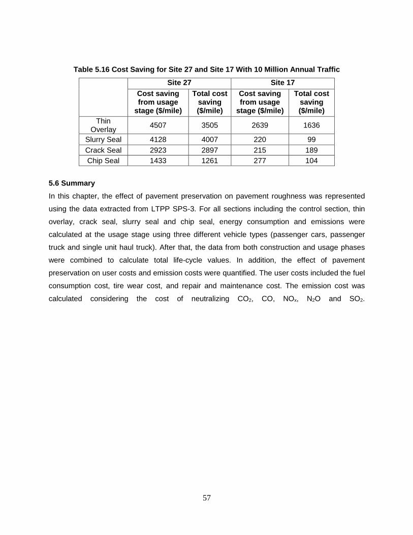
57

Table 5.16 Cost Saving for Site 27 and Site 17 With 10 Million Annual Traffic

Site 27 Site 17

Cost saving from usage

stage ($/mile)

Total cost saving ($/mile)

Cost saving from usage

stage ($/mile)

Total cost saving ($/mile)

Thin Overlay

4507 3505 2639 1636

Slurry Seal 4128 4007 220 99

Crack Seal 2923 2897 215 189

Chip Seal 1433 1261 277 104

5.6 Summary

In this chapter, the effect of pavement preservation on pavement roughness was represented

using the data extracted from LTPP SPS-3. For all sections including the control section, thin

overlay, crack seal, slurry seal and chip seal, energy consumption and emissions were

calculated at the usage stage using three different vehicle types (passenger cars, passenger

truck and single unit haul truck). After that, the data from both construction and usage phases

were combined to calculate total life-cycle values. In addition, the effect of pavement

preservation on user costs and emission costs were quantified. The user costs included the fuel

consumption cost, tire wear cost, and repair and maintenance cost. The emission cost was

calculated considering the cost of neutralizing CO2, CO, NOx, N2O and SO2.

58

Chapter 6 CONCLUSIONS AND RECOMMENDATIONS

6.1 Major Findings

In this study, energy and emissions of four pavement preservation treatments were quantified at

the construction and usage stages. At the usage stage, pavement surface characteristics and

vehicle factors were considered in the analysis of vehicle fuel consumption and emissions. The

HDM-4 Model and the MOVES 2010 EPA model were used to consider the effect of pavement

roughness on fuel consumption (energy consumed) and emissions. Major findings are as

follows:

1. The thin overlay was found to have the highest energy consumption and emissions

among four preservation treatments during construction stage. If only construction

stage is considered, energy and emissions are ruled by use of amount of material

and manufacture process.

2. The effect of pavement surface characteristics (roughness, texture, and deflection)

on fuel consumption and emissions varies depending on vehicle type.

3. Among four preservation treatments, the thin overlay resulted in the greatest

reduction of energy consumption and emission at usage stage due to improvement

of pavement surface smoothness when compared to the control section.

4. The reductions of GHG emission at usage stage are much greater than the GHG

emission produced at construction stage for all preservation treatments. Excluding

the usage stage will omit the fact that construction stage has less impact on

pavement LCA than usage stage. Combining both construction and usage stages

gave a life-cycle impact of pavement preservation on energy and GHG emission.

5. The effect of pavement roughness on user cost was more significant than on

emission cost. This indicates that the user cost cannot be neglected when

quantifying the benefit of pavement preservation.

In summary, this whole study provides a deep insight of including usage stage in life

cycle assessment of pavement. The results show that there is a significant amount of

change in energy consumption and emissions when traffic factors and pavement surface

characteristics are considered during usage stage.

59

6.2 Future Research Recommendations

1. Only four pavement preservation treatments were considered in this study, future

studies should include other preservation and rehabilitation techniques to get a

broader view on this subject, such as micro-surfacing, milling and overlay.

2. More construction materials like cold mix asphalt, warm mix asphalt, reclaimed

asphalt pavement and rubber sealant should be included in future studies.

3. The analysis period was fixed for preservation treatments considered in this study. In

future studies multiple preservation treatments applied at different timing in the

pavement life cycle should be considered.

4. In addition to pavement roughness, other factors like albedo, concrete carbonation,

leachate etc., should be considered at usage stage of LCA.

60

REFERENCES

AASHTO. (2005). “Roadway Lighting Design Guide”. American Association of State Highway

and Transportation Officials. Washington, DC.

American Concrete Pavement Association, (ACPA). (2002). “Albedo: A Measure of Pavement

Surface Reflectance”. Concrete Pavement Research & Technology, Issue 3.05, 1-2.

Akbarian, M., Franz-Josef Ulm. (2012). “Model Based Pavement-Vehicle Interaction Simulation

for Life Cycle Assessment of Pavements”. Thesis (S.M.), Dept. of Civil and Environmental

Engineering, Massachusetts Institute of Technology.

Ardekani, S., and Sumitsawan P., (2010). “Effect of Pavement Type on Fuel Consumption and

Emissions in City Driving”. Department of Civil Engineering, The University of Texas at

Arlington, Arlington, TX, 4-32.

Bennett, C. R, and Greenwood, I. D. (2003). “Modeling Road User and Environmental Effects in

HDM-4”. Version 3.0. International Study of Highway Development and Management Tools

(ISOHDM), World Road Association (PIARC), Cedex, France.

Berthiaume, R., and Bouchard, C., (1999). “Exergy Analysis Of The Environmental Impact of

Paving Material Manufacture”. Trans Can Soc Mech Eng;23, 96-187.

Beuving, E., De Jonghe, T., Goos, D., Lindhal, T., Stawiarski, A. (2004). “Environmental Impacts

and Fuel Efficiency of Road Pavements”. Europe Asphalt Pavement Association and

Eurobitume, 4-21.

Carlson, A. (2011). “Life Cycle Assessment of Roads and Pavement- Studies Made in Europe”.

VTI Rapport 736A, 9-19.

Carvalho, R., Ayres, M., Shirazi, H., Selezneva, O., and Darter, M. (2011). “Impact of Design

Features on Pavement Response and Performance in Rehabilitated Flexible and Rigid

Pavements”. Federal Highway Administration (FHWA), FHWA-HRT-10-066, pp 78-102.

Cass, D., Mukherjee, A. (2011). “Calculation of Greenhouse Gas Emissions for Highway

Construction Operation by Using a Hybrid Life Cycle Assessment Approach: Case Study for

Pavement Operations”. Journal of Construction Engineering and Management ASCE pp. 1-11.

61

Copple, F. (1981). “Cost and Energy Consideration”. National Seminar on PCC Pavement

Recycling and Rehabilitation. Transportation Research Board, 134-139

Chatti, K. Zaabar, I. (2012). "Estimating the Effects of Pavement Condition on Vehicle Operating

Costs". Transportation Research Board, Washington, D.C.

Chan, W.C. (2007). “Economic and Environmental Evaluations of Life-Cycle Cost Analysis

Practices”. A Case Study of Michigan DOT Pavement Projects. University of Michigan, Ann

Arbor, USA.

Chappat, M. and Bilal, J. (2003). “The Environmental Road of the Future: Life Cycle Analysis”.

Energy Consumption and Greenhouse Gas Emissions. Colas Group, 2-34.

Chehvoits, J., Galehouse, L. (2010). “Energy Usage and Greenhouse Gas Emissions of

Pavement Preservation Processes for Asphalt Concrete Pavements”. First International

Conference on Pavement Preservation, Transportation Research Board, 27-42.

Chui, T., Hsu, T., and Yang, W., (2008). “Life Cycle Assessment On Using Recycled Materials

For Rehabilitating Asphalt Pavements”. Resources, Conservation and Recycling 52, 545–

556.Eurobitume. (2012). “Life Cycle Inventory: Bitumen 2nd Edition July”. European Bitumen

Association. Brussels, Belgium. 4-31

Guistizzo, F. (2011). “Preventive Maintenance Treatments on Road Pavements: Multi-Approach

Life-Cycle Assessment”. Politecnico Di Milano.

Hakkinen, T., Makela, K. (1996). “Environmental Impact of Concrete and Asphalt Pavements in

Environmental Adaptation of Concrete”. Technical Research Center of Finland, 56-67.

Hassan, M. M. (2009). “Life-Cycle Assessment of Warm-Mix Asphalt: An Environmental and

Economic Perspective”. Transportation Research Board, 1-15.

Hoang, T., Jullien, A. and Ventura, A. (2005). “A Global Methodology for Sustainable Road –

Application to The Environmental Assessment of French Highway”. 10th International

Conference on Durability of Buildings Materials and Components, April 17th - 20th, Lyon, 1-10.

International Slurry Surfacing Association (ISSA). (2010).” Recommended Performance

Guideline for Emulsified Asphalt Slurry Seal”, A105, 2-16.

62

Haugodegard, T., J. Johansen, D. Bertelsen, and K. Gabestad. (1994). “Norwegian Public

Roads Administration: A Complete Pavement Management System in Operation”. Third

International Conference on Managing Pavements, San Antonio, Vol. 2, Transportation

Research Board , National Research Council, Washington, D.C.

Horvath, A. and Hendrickson, C. (1998). “Comparison of Environmental Implications of Asphalt

and Steel-Reinforced Concrete Pavements”. Transportation Research Record. Vol.1626, 105-

113.

Huang, Y., Bird, R., and Margaret, B. (2009). “A Comparative Study of The Emission By Road

Maintenance Works And The Disrupted Traffic Using Life Cycle Assessment And Micro

Simulation”. Transportation Research Part D: Transport and Environment, Volume 14, Issue

3,197–204.

Huang, Y., Bird, R., and Heidrich, O. (2008). “Development of A Life Cycle Assessment Tool For

Construction And Maintenance of Asphalt Pavements”. Journal of Cleaner Production 17, 283–

296.

ISO 14040, (1997). “Environmental Management – Life Cycle Assessment – Principles and

Framework”. American National Standards Institute, International Organization for

Standardization, Geneva, 1-7.

Islam, S., Butlar, W., (2012). “Effect of Pavement Roughness on User Costs”. Transportation

Research Record: Journal of the Transportation Research Board,No. 2285, pp 47-55.

Kalman, B. (2013). “RE-ROAD – End of Life Strategies of Asphalt Pavements”. re-

road.fehrl.org/.

Kendall, A., G. A. Keoleian, & G. E. Helfand. (2005) “Integrated Life-Cycle Assessment and Life-

23 Cycle Cost Analysis Model for Concrete Bridge Deck Applications”. Journal of Infrastructure

24 Systems, Vol. 14, No. 3, 2008, pp. 214-222.

Kralsson, R., Carlson, A., and Dolk E. (2012). “Energy Use Generated By Traffic and Pavement

Maintenance”. www.vti.se/publications.

63

Kristjánsdóttir, Ó., Muench, T.S., Michael, L., and Burke, G. (2007). “Assessing Potential for

Warm-Mix Asphalt Technology Adoption”. Transportation Research Record: Journal of the

Transportation Research Board, 91–99.

Leng, Z., and Imad, A. (2011). “Comparative Life Cycle Assessment Between Warm SMA and

Conventional SMA”. Research Report ICT-11-090, Illinois Center for Transportation Series no.

11-090, 4-16.

Lee, N., (2012). “Benefits in Energy Savings and CO2 Reduction by using Reclaimed Asphalt

Pavement”. Transportation Research Board, 2012 Annual Meeting, 2-18.

Lippiatt, C. B. (2007). “Building for Environmental and Economic Sustainability Technical

Manual and User Guide”. National Institute of Standards and Technology, Gaithersburg, MD.

307p.

Lu, P. and Tolliver, D. (2012). “Pavement Treatment Short-Term Effectiveness in IRI Change

Using Long-Term Pavement Program Data”. J. Transp. Eng., 138(11), 1297–1302.

Mallela, J. and Sadasivam, S. (2011). “Work Zone Road User Costs – Concepts and

Applications”. FHWA-DTFH61-06-D-00004,Federal Highway Administration, Washington, DC.

Marceau, M.L., Nisbet, M.A., and Van Geem, M.G. (2007). “Life Cycle Inventory of Portland

Cement Concrete”. Portland Cement Concrete Association. Skokie. 118p.

Maintenance Technical Advisory Guide (MTAG), (2003) State of California Department of

Transportation.

McGhee K K., and Flintsch G W., (2003). “High-Speed Texture Measurement of Pavements”.

Virginia Transportation Research Council. Charlottesville, Virginia USA, 3-23.

Milachowski, C., Stengel, T., and Gehlen, C. (2012). “Life Cycle Assessment for Roads

Construction and Use”. Center for Building Material, Techische University Munchen, Germany,

3-18.

Morosiuk, G., Riley, M. and Toole, T., (2002) HDM-4 Highway Development &

Management.Volume Two, Application Guide.PIARC, World Road Association. 2-133.

64

Motor Vehicle Emission Simulator (MOVES) (2012). “User Guide for MOVES2010b”. U.S.

Environmental Protection Agency (EPA), 2-101.

Mroueh, U.M., Mäkelä, E., Wahlström, M., Kauppila, J., Sorvari, J., Heikkinen, P.,Salminen, R.,

Juvankoski, M., and Tammirinne, M., (2000). “By-Products in Earth Construction: Assessment

of Acceptability”. National Technology Agency. Technology Review 96/2000.

Muench, T. S. (2010). “Roadway Construction Sustainability Impacts- Review of Life-Cycle

Assessments”. Transportation Research Record: Journal of the Transportation Research Board,

No. 2151, 36–45.

National Technology Development, LLC. (2009). “Quantify the Energy and Environmental

Effects of Using Recycled Asphalt and Recycled Concrete for Pavement Construction. Phase I

Final Report”. Albany (NY), USA, Report No.: C-08-02, 2-46.

Noellette, Conway-Schempf. (1998). “Case Study: Economic Input-Output Life Cycle

Assessment of Asphalt versus Steel Reinforced Concrete for Pavement Construction”. ,

Pittusburg, PA. 2-12.

Nisbet, MA., Marceau, ML., VanGeem, MG., and Gajda, J., (2001). “Environmental Life Cycle

Inventory Of Portland Cement Concrete And Asphalt Concrete Pavements”. Portland Cement

Association. Skokie, IL . PCA R&D Serial No. 2489.

Park, K., Hwang, Y., Seo, S., and Seo, H., (2003). “Quantitative Assessment of Environmental

Impacts on Life Cycle of Highways”. J Construct Eng Manage,129, 25–31.

Roudebush, WH., (1999). “Environmental Value Engineering Assessment of Concrete and

Asphalt Pavement”. Portland Cement Association Skokie, IL.

Said, D., Trusty, B. W., Geomans, C., Finlayson, G., and Portalupi, F. (2011). “Life Cycle

Assessment Of Roadways Using A Pavement Sustainability Too”l. Transportation Research

Board 91st Annual Meeting, Washington, DC, 15p.

Santero, N., Masanet, E., and Horvath, A. (2011). “Life-Cycle Assessment of Pavements Part II:

Filling The Research Gaps”. Resources, Conservation and Recycling 55, 810–818.

Santero, N., and Horvath, A. (2009). “Global Warming Potential of Pavements”. Department of

Civil and Environmental Engineering, University of California, Berkely, 2-7.

65

Santero, N., Masanet, E., and Horvath, A. (2011). “Life-Cycle Assessment of Pavements. Part I:

Critical review”. Resources, Conservation and Recycling, 55(9), 801-809.

Santero, N., Loijos, A., Akbarian, M., and Ochsendorf, J. (2011). Methods, Impacts and

Opportunities in the Concrete Pavement Life Cycle. Concrete Sustainability Hub Massachusetts

Institute of Technology, 15-55.

Santero, N., Loijos, A., Akbarian, and M., Ochsendorf, J. (2011). “Methods, Impacts, and

Opportunities in the Concrete Pavement Life Cycle”. Massachusetts Institute of Technology.

MA, 13-23.

Santero, N., Masanet, E., & Horvath, A. (2011). “Life-Cycle Assessment of Pavements. Part I:

Critical Review”. Resources, Conservation and Recycling, 55(9), 801-809.

Stripple, H. (2001). “Life Cycle Assessment of Road, A Pilot Study for Inventory Analysis”,

Second Revised Edition. IVL Swedish National Road Administration. Gothenburg, Sweden. 96p.

Sweeney, A., West, R.P., and O’Connor C. (2011). “Parameters Affecting The Albedo Effect in

Concrete”. Department of Civil, Structural and Environmental Engineering, Trinity College,

Dublin 2, Ireland, 1-8.

Tatri, O., Nazzal, M., and Kucukvar, M. (2011). “Comparative Sustainability Assessment of

Warm-Mix Asphalts: A Thermodynamic Based Hybrid Life Cycle Analysis”. Resources,

Conservation and Recycling Volume 58, 18–24

Theonux, et al. (2006). “Energy Consumption Comparison For Different Asphalt Pavements

Rehabilitation Techniques used in Chile”. Resources, Conservation and Recycling 49, 325–339.

Victor, C. Li. (2003). “Durable Overlay Systems with Engineered Cementitious Composites”.

International Journal for Restoration of Buildings and Monuments Vol. 9, No 2, 215-234.

Wang, T., Lee, I., Kendall, A., Harvery, A., Lee E., Kim C. (2013). “UCPRC Life Cycle

Assessment Methodology and Initial Case Studies on Energy Consumption and GHG

Emissions for Pavement Preservation Treatments with Different Rolling Resistance”. University

of California Pavement Research Center UC Davis, UC Berkeley, 144p.

Wang, T., Lee I., Kendall A., Harvery A., and Lee E., Kim C. (2012). “Life Cycle Energy

Consumption and GHG Emission from Pavement Rehabilitation with Different Rolling

Resistance”. Journal of cleaner production 33. 89-96

66

Wang, Y., Wang, G., and Mastin, N. (2012). “Costs and Effectiveness of Flexible Pavement

Treatments: Experience and Evidence”. J. Perform. Constr. Facil., 26(4), 516–525.

Weiland, C., Muench, S. (2010). “Life Cycle Assessment of Portland Cement Concrete

Interstate Highway Rehabilitation and Replacement”. Washington State Department of

Transportation Research Report, 105p.

Weiland, C., and Muench, S. (2010). “Life-Cycle Assessment of Reconstruction Options for

Interstate Highway Pavement in Seattle, Washington”. Transportation Research Board of the

National Academies, Washington, D.C, 18–27.

Yanowitz, J., McCormick, R. L., & Graboski, M. S. (2000). “In-Use Emissions From Heavy-Duty

Diesel Vehicles”. Environmental Science & Technology, 34(5), 729-740

Yu, B., Lu, Q. (2011). “Life Cycle Assessment of Pavement Overlay Systems with Focus on

Usage phase”. Transportation research part D, 380-388.

Yu, B., and Lu, Q., (2012). “Life Cycle Assessment of Pavements: Methodology and Case

Study”. Transportation Research Part D 17,380–388.

Zaabar, I., Chatti, K., 2010. “Calibration of HDM-4 Models for Estimating the Effect of Pavement

Roughness on Fuel Consumption for U.S. Conditions”. Transportation Research Record:

Journal of the Transportation Research Board, 105-116.

Zaabar, I., Chatti, K., 2012. “Estimating the Effect of Pavement Conditions on Vehicle Operating

Costs”. National Cooperative Highway Research Program, Report 720. Transportation

Research Board, 50-57.

Zaniewski, J. P., Butler, B. C., Cunningham, G. E., Elkins, G. E., Paggi, M. S., and Machemehl,

R. (1982). “Vehicle Operating Costs, Fuel Consumption, and Pavement Type and Condition

Factors”. U.S. Department of Transportation, Federal Highway Administration Washington

D.C.375p.

Zaniewski, JP. (1989). “Effect of Pavement Surface Type on Fuel Consumption”. Portland

Cement Association, PCA Skokie, IL, 1-4.

67

Zhang, H., Keoleian, A G. and Lepech, M.D. (2008). “An Integrated Life Cycle Assessment and

Life Cycle Analysis Model for Pavement Overlay Systems”. Life-Cycle Civil Engineering –

Biondini & Frangopol (eds),Taylor & Francis Group, London, 1-5.

Zhang, H., Keoleian, A.G., Lepech, D. M., and Kendall, A. (2010). “Life-Cycle Optimization of

Pavement Overlay Systems”. Journal of Infrastructure Systems Vol. 16, No. 4, 310-322.

Zhang, H. (2009). “Sustainable Pavement Asset Management Based on Life Cycle Models and

Optimization Methods”. Doctoral Dissertation, University of Michigan, Ann Arbor, 1- 125.