Leverage, Default, and Forgiveness: Lessons from the ...dido.econ.yale.edu/~gean/art/p1419.pdf · Leverage, Default, and Forgiveness: ... limitation, hampering the ability of the

LEVERAGE, DEFAULT, AND FORGIVENESS: LESSONS FROM THE AMERICAN AND EUROPEAN CRISES

by

John Geanakoplos

COWLES FOUNDATION PAPER NO. 1419

COWLES FOUNDATION FOR RESEARCH IN ECONOMICS YALE UNIVERSITY

Box 208281 New Haven, Connecticut 06520-8281

2014

http://cowles.econ.yale.edu/

Journal of Macroeconomics 39 (2014) 313–333

Contents lists available at ScienceDirect

Journal of Macroeconomics

journal homepage: www.elsevier .com/locate / jmacro

Leverage, Default, and Forgiveness: Lessons from the Americanand European Crises

http://dx.doi.org/10.1016/j.jmacro.2014.01.0010164-0704/� 2014 Elsevier Inc. All rights reserved.

⇑ Address: Department of Economics, Yale University, Box 208281, New Haven, CT 06520-8281, United States.E-mail address: [email protected]

John Geanakoplos ⇑Yale University, United StatesSanta Fe Institute, United States

a r t i c l e i n f o

Article history:Available online 19 February 2014

JEL classification:G01G18E44

Keywords:Leverage cycleAmerican and European crisesCredit surfaceDebt forgiveness

a b s t r a c t

This paper argues that macroeconomic stability depends less on riskless interest rates thanon leverage and other measures of credit conditions, like average FICO scores of borrowers.It suggests that the leverage cycle played a central role in the recent American and Europeanfinancial crisis. In the leverage cycle, asset prices and leverage rise when volatility is low andthen fall as volatility rises. Sometimes asset prices fall so far below debt levels that it wouldbe better for everybody if debt were partially forgiven. The paper recommends that centralbanks regularly monitor and forecast the whole credit surface, and in extreme casesintervene to regulate risky interest rates and impose partial debt forgiveness.

� 2014 Elsevier Inc. All rights reserved.

1. Introduction: The credit surface

The American debt crisis that began in February 2007 with the collapse of the subprime mortgage market is now nearlyseven years old. The European debt crisis that began in late 2009 in Greece is now over four years old. That two such majordebt crises could occur and be so slow to cure suggests that the models and tools policymakers and central bankers havetraditionally used before and even after the crisis need to be reconsidered.

Central bankers talk about many aspects of the economy, but when it comes to action, they essentially concernthemselves exclusively with the short term riskless interest rate. Recently, in what is regarded as a radical departure thatproves the point, they have tried to influence expectations of future short term riskless interest rates via forward guidanceand the purchase of long term assets. This age old preoccupation with riskless interest rates seems to me an old fashionedlimitation, hampering the ability of the central banks to prevent crises and to help extricate economies from their aftermath.

I believe that credit plays a central role in the booms and busts of market economies, and even in milder fluctuations. But Ido not believe that the credit conditions influencing booms and busts are driven primarily by fluctuations in riskless interestrates, or by the wrong riskless interest rates. When bankers say credit is tight, they do not simply mean that riskless interestrates are so high they are choking off demand for loans. They mean that many businesses and households who would like toborrow at the current riskless interest rates cannot get a loan. They are referring to the supply side of the credit market, notjust the demand side.

http://crossmark.crossref.org/dialog/?doi=10.1016/j.jmacro.2014.01.001&domain=pdf

http://dx.doi.org/10.1016/j.jmacro.2014.01.001

mailto:[email protected]

http://dx.doi.org/10.1016/j.jmacro.2014.01.001

http://www.sciencedirect.com/science/journal/01640704

http://www.elsevier.com/locate/jmacro

314 J. Geanakoplos / Journal of Macroeconomics 39 (2014) 313–333

The reason some borrowers cannot get a loan at the same (riskless) interest rate that others do is that their lenders areafraid they may default. Risky interest rates (or spreads to riskless interest rates on loans that might default) are often moreimportant indicators of economic conditions than riskless interest rates. Nevertheless, central bankers have paid scant atten-tion to default in their macroeconomic models.1 In my opinion, central banks should pay attention to, and influence, riskyinterest rates if they want to preserve financial stability.

When lenders are afraid of default they often ask for collateral to secure their loans. How much collateral they require is acrucial variable in the economy called the collateral rate or leverage. Lenders also worry about the credit worthiness of theborrowers, which in the case of households is often represented by their FICO credit score.2 The credit conditions of the econ-omy cannot be summarized accurately by a single riskless interest rate, but rather by an entire surface, where the offered inter-est rate from lenders can be thought of as a function of the collateral and the FICO score: r = f(collateral, FICO).3 The higher thecollateral, or the higher the FICO, the lower will be the interest rate. For sufficiently high collateral and FICO, the interest ratemay stabilize at a constant called the riskless interest rate. If we compare two different economic climates, represented by twodifferent surfaces f and g, it might well be the case that both of them give precisely the same riskless interest rate, but never-theless g depicts much tighter credit conditions than f. For example in g the riskless interest rate might only be attained withmuch higher levels of collateral and FICO.

In my opinion, central banks should be trying to estimate the existing credit surfaces on a monthly basis. They could getthe data to do much of this if they looked at individual transactions to see how the rates change as the terms change. Part ofthe surface would have to be estimated by extrapolation, since it covers conditions at which no trades (or only a few trades)are observed. Estimating these surfaces explicitly would bring much clarity to the general credit climate. But much moreimportantly, it would force policy makers to predict what effect their interventions would have on the whole surface, notjust on the riskless interest rate. How clearly did the United States Federal Reserve Board of Governors understand thatits recent policy of Quantitative Easing (achieved partly by buying agency mortgages) would dramatically loosen the creditsurface for high yield bonds, but provide very little loosening in the credit surface for mortgage borrowers with average cred-it scores? In my opinion, policymaking would be enormously sharpened if it were disciplined by the question of the wholecredit surface.4

The theory of asset pricing is one area that would be radically improved by considerations of the credit surface. Econo-mists as far back as Irving Fisher have understood that the riskless interest rate influences the price of an asset by changingthe expected present value of its dividends, or its fundamental value. But economists have not sufficiently appreciated thatthe rest of the credit surface also influences risky asset prices: the looser the credit surface, the higher the asset prices of thecorresponding risky assets.

The riskless interest rates depend on the impatience of the agents in the economy, and on the expectations of futuregrowth, among other factors. The movements in the rest of the credit surface are driven primarily by the risk tolerance ofborrowers and lenders’ fears of default, in addition to the conventional determinants like impatience and growth, whichapply with or without uncertainty. The probability of default in turn depends on at least two factors: one is the volatilityof collateral prices, and the other is the indebtedness of the borrowers.

The higher the volatility of collateral prices (at least in the down tail), the more insecure the lenders will feel and the high-er the interest rate they will insist on for the same collateral. The higher the indebtedness of the borrowers, the less likelythey will be willing or able to repay a new loan, and the more insecure lenders will become. Higher volatility and higherindebtedness makes for a tighter credit climate.

If a very tight credit climate is unhealthy for the economic environment, then we are led to two radical sounding conclu-sions. First, central banks should intervene not only by influencing the riskless interest rate (fully cognizant of the indirecteffects on the rest of the credit surface, as we mentioned earlier), but also by directly influencing risky debt. In one direction,central banks could tighten overly hot credit markets by for example prohibiting loans at LTV exceeding some threshold, asthe Bank of Israel did in 2010 by banning mortgage loans at LTV above 60%. In the other direction, a central bank couldextend credit to borrowers at terms that no private investor would provide, as the Fed did in 2009, lending 95 cents againsta dollar’s worth of credit card collateral, and student loan collateral, and car loan collateral. The ECB has done the same withsovereign debt. Second, in extreme environments, such as the United States faced in 2007–2009, and as Europe faces now,debt forgiveness could also figure into the policy mix of central banks. Once it is admitted that there may be defaults againstthe central bank, one can consider the idea of partial forgiveness.5 I shall try to argue that in extreme circumstances, properlyimplemented forgiveness can actually recover more money for the lender, without creating any moral hazard for present orfuture borrowers. The stigma against default is so strong, that it has stymied rational discussion about forgiveness.

1 Of course central bankers pay a great deal of attention to the solvency of individual banks, but when it comes to their macroeconomic forecasts of demandand growth, it is my impression that default does not figure in.

2 FICO is a private company that provides credit scores to financial institutions to help them in their decision making. The FICO score is not the perfectrepresentation of credit worthiness. Ideally one would like a measure that represented the willingness of the borrower to repay even if there was no collateral,which would depend on the ratio between the internal penalty (in lost reputation and embarrassment, etc.) and the marginal utility of consumption or wealth.

3 There should be a different credit surface for each maturity. One could also imagine adding more variables beyond collateral and credit worthiness, such asdebt to income or debt to wealth.

4 This might lead to a whole new kind of policy, tailored to specific kinds of borrowers.5 In my view, in extreme situations policy makers should consider imposing debt forgiveness on private lenders, as well as extending debt forgiveness

themselves.

J. Geanakoplos / Journal of Macroeconomics 39 (2014) 313–333 315

I am fully aware that my notions of monitoring and forecasting the credit surface, influencing risky interest rates, andpartial debt forgiveness will not be accepted uncritically. Rather than presenting a formal model to make my case, I shalldescribe the ongoing American financial crisis, and briefly the European crisis, in terms of leverage, default, and the failureto forgive.

2. My Wall Street experiences

In the calendar year 1990 I decided to spend my Yale sabbatical at the Wall Street investment bank Kidder Peabody. As atheoretical economist I wanted to see what models real world practitioners used. Among other things, I learned for the firsttime about the securitization and tranching of mortgages. At the end of my sabbatical year, the head of Kidder’s Fixed IncomeDepartment asked me if I would help him hire a new, more mathematical research department. After I returned to Yale hesuggested that since I had hired all the people, I could lead its research direction from Yale, while leaving the details to theheads of the various divisions I had created. In those years Kidder Peabody became the dominant investment bank in themortgage market. This situation kept me thinking about collateral and the omnipresent role it played on Wall Street, at leastin fixed income markets. I realized that collateral and the potential for default were at the heart of financial transactions; yetneither collateral nor default appeared in any macroeconomic textbook I ever saw. In 1997 I published my paper ‘‘PromisesPromises’’ introducing collateral equilibrium. In that paper I showed the way supply and demand could determine leverageas well as interest rates, and I showed that assets like houses that were good collateral would be priced higher (and some-times too high) because they provided an additional service of facilitating borrowing.

In 1994 Kidder Peabody went out of business after 135 years as a result of a scandal in the government bond tradingdepartment. I didn’t quite realize it at the time, but the precipitating cause of the crisis was the bottom of a leverage cyclein Treasuries. I had to rush down to Kidder from Yale and call into my office each of the 75 people in the research departmentand say you’re fired. Then I got up and went into the office next door and the guy said to me you’re fired.

Michael Vranos, the head of Kidder’s mortgage operation, and five more of us, decided to found a hedge fund called Elling-ton Capital Management that would buy the very same mortgage securities that Kidder and the other Wall Street firms hadbeen creating. After the leverage cycle crisis of 1994, we made tremendous returns at Ellington. But at the end of 1997another gigantic collapse, this time in emerging markets and in mortgages, brought down the famous hedge fund Long TermCapital. Two of its principals had just won the Nobel Prize in economics earlier that year. We ourselves at Ellington got amargin call that put us in jeopardy. We survived our crisis, and made tremendous returns for our investors just after the cri-sis, as we had just after the crisis in 1995. But it got me wondering what caused these ups and downs that had nearlywrecked the fixed income markets twice in five years? I presented my theory of the leverage cycle at the World Congressof the Econometric Society in 2000, which was published in the conference volume in 2003.6 I extended my analysis to multi-ple leverage cycles with my student Ana Fostel in a 2008 paper. All three of these papers were written before the current crisis.In 2010 and 2012 I published papers suggesting that the American crisis of 2007–2009 was another example of the leveragecycle. In the current paper I summarize these papers. I think the most recent crisis in the United States and in Europe is similarin many respects to the crises of 1994 and 1998, just bigger. From this later perspective, looking back on all three crises, I drawlessons for central banks about how to avoid another big leverage cycle crisis. I believe that a crisis is normal writ large, and solessons from crises are lessons for normal times as well.

3. Equilibrium leverage and volatility

Traditionally, governments, economists, as well as the general public and the press, have regarded the riskless interestrate as the most important policy variable in the economy. Whenever the economy slows, the press clamors for lower inter-est rates from the Federal Reserve, and the Fed often obliges. But sometimes, especially in times of crisis, collateral rates(equivalently, margins or leverage) are far more important than interest rates.

The use of collateral and leverage is widespread. A homeowner (or a big investment bank or hedge fund) can often spend$20 of his own cash to buy an asset like a house for $100 by taking out a loan for the remaining $80 using the house as col-lateral. In that case, we say that the margin or haircut or down payment is 20%, the loan to value (LTV) is $80/$100 = 80%, andthe collateral rate is $100/$80 or 125%. The leverage is the reciprocal of the margin, namely, the ratio of the asset value to thecash needed to purchase it, or $100/$20 = 5. All of these ratios are different ways of saying the same thing.

In standard economic theory, the equilibrium of supply and demand determines the interest rate on loans. But in real life,when somebody takes out a secured loan, he must negotiate two things: the interest rate and the collateral rate. A propertheory of economic equilibrium must explain both. Standard economic theory has not really come to grips with this problemfor the simple reason that it seems intractable: how can one supply-equals-demand equation for a loan determine two vari-ables – the interest rate and the collateral rate?

In Geanakoplos (1997) and Dubey et al. (2005) I showed how supply and demand do indeed determine both. Moreover, Ishowed how the two variables are influenced in the equilibration of supply and demand mainly by two different factors: the

6 See Geanakoplos (2003). Ana Fostel and I coined the phrase Leverage Cycle in Fostel–Geanakoplos (2008).


interest rate reflects the underlying impatience of borrowers, and the collateral rate reflects the perceived volatility of assetprices and the resulting uncertainty of lenders about default.7

The key to understanding the endogenous choice of leverage is to realize that there is a menu of potential loans, indexedby the collateral and the amount promised. If the credit worthiness of the borrower is observable, that will also figure intothe menu.8 Each potential loan will be priced in equilibrium, possibly all at different prices. For each potential loan, there is aseparate supply and demand equation which fixes its price. The paradox of one equation and two variables is resolved by notic-ing that there are exactly as many supply equals demand equations as there are kinds of loans and as there are prices. This givesthe credit surface described in the introduction.

An agent who wishes to borrow more can do so by increasing his promise on the same collateral, or by putting up morecollateral. In the former case he will face a worse price, that is, he will have to pay a higher interest rate, because lenders willbe more concerned about default. In the latter case he has to be willing to own and hold the extra collateral, which he mightnot want to do. Thus some borrowers might be constrained in equilibrium: they would like to borrow more at the sameinterest rate but cannot do so. This credit rationing is the reason we speak of tight or loose credit markets.

Each potential loan trades at a well-defined loan to value in equilibrium: the LTV of the loan is defined as the equilibriumprice of the loan divided by the equilibrium price of the collateral specified by the loan. The LTV of the collateral is the aver-age LTV over all loans backed by the same collateral. For example, if one borrower takes out a loan of $160 on his $200 house,while another (subprime) borrower takes out a loan of $98 on his $100 houser, then the average LTV on housing is86% = $258/$300. Some buyers purchase their homes with no debt at all. If we include these houses in the denominator,we get what is called the diluted LTV for the collateral. Investor leverage also emerges in equilibrium as the total amountborrowed over the total value of the assets owned by the investor.9

Sometimes the same collateral can back loans of different amounts, as we saw in the housing market where primeborrowers generally took out loans at lower LTVs than subprime borrowers. But at other times it seems that all borrowerssettle on a focal LTV, as in the early 1990s when the vast majority of borrowers seemed to take on 80% LTV housing loans. InFostel–Geanakoplos (2013) we showed that when there are only two possible future events each period, every financial assetwill back just one LTV loan in equilibrium. In this case of binomial economies, Fostel and Geanakoplos (2013) prove thatequilibrium LTV will always be determined by the worst case return of the asset. Under some conditions margins areproportional to the volatility of asset payoffs: the lower the volatility, the higher the leverage, and the higher the volatilityof the asset price, the lower the leverage on the asset.10

4. Leverage and asset prices

Practitioners, if not economists, have long recognized the importance of collateral and leverage. For a Wall Street trader,leverage is important for two reasons. The first is that if he is leveraged k times, then a 1% change in the value of the collateralmeans a k percent change in the value of his capital. (If the house in our example goes from $100 to $101, then after selling thehouse at $101 and repaying the $80 loan, the investor is left with $21 of cash on his $20 investment, a 5% return.) Leverage thusmakes returns riskier, either for better or for worse. Second, a borrower knows that if there is no-recourse collateral, so that hecan walk away from his loan after giving up the collateral without further penalty, then his downside is limited. The most theborrower can lose on the house loan is his $20 of cash, even if the house falls in value all the way to $0 and the lender loses $80.No-recourse collateral thus effectively gives the borrower a put option (to ‘‘sell’’ the house for the loan amount). Recently, sev-eral commentators have linked leverage to the crisis, arguing that if banks were not so leveraged in their borrowing theywould not have lost so much money when prices went down, and that if homeowners were not so leveraged, they wouldnot be so far underwater now and so tempted to exercise their put option by walking away from their house. Of course, thesetwo points are central to my own leverage cycle theory; I discuss them in more detail later. But there is another, deeper pointto my theory, that was not commonly understood by traders, which I think is the real story of leverage.

The main implication of my leverage cycle theory is that when leverage goes up, asset prices go up and when leveragegoes down, asset prices go down.11 For many assets, there is a class of natural buyers or optimists who are willing to pay muchmore for the asset than the rest of the public. They may be more risk-tolerant; or they may simply be more optimistic; or theymay get more utility from holding the collateral, as, for example, with housing.12 If they can get their hands on more money

7 Another factor influencing leverage in the long run is the degree of financial innovation. Since scarce collateral is often an important limiting factor, theeconomy will gradually devise ways of stretching the collateral, by tranching (so the same collateral backs several loans) and pyramiding loans (so the samecollateral can be used over and over to back loans backed by loans).

8 Other factors, such as the ratio of debt to wealth (or income) of the borrower, might also play a role in defining the loan.9 In conventional models of borrowing, leverage also emerges in equilibrium. The difference is that in those older models leverage is determined entirely by

how many loans the borrowers want to take at the fixed equilibrium interest rate. In my theory the equilibrium interest rate changes as the LTV changes, so thelending terms play a much more significant role in constraining the choices of borrowers.

10 Investor leverage, like diluted leverage, is more complicated than asset leverage even in binomial economies because of the possibility that some borrowersmight not fully use all their assets as collateral for loans.

11 Leverage is like more money in making prices go up, but unlike money it affects only prices of goods that can serve as collateral; printing more money tendsto increase all prices, including food and other perishables.

12 Two additional sources of heterogeneity are that some investors are more expert at hedging assets, and that some investors can more easily obtain theinformation (like loan-level data) and expertise needed to evaluate the assets.

Fig. 1. Marginal buyer theory of price.


through borrowing, they will spend it on the assets and drive those asset prices up. If they lose wealth, or lose the ability toborrow, they will be able to buy less of the asset, and the asset will fall into more pessimistic hands and be valued less.

It is useful to think of the potential investors arrayed on a vertical continuum, in descending order according to their will-ingness to buy, with the most enthusiastic buyers at the top (see Fig. 1). Whatever the price, those at the top of the contin-uum above a threshold will value the asset more than the price and become buyers, while those below will value it less, andsell. The marginal buyer is the agent at the threshold on the cusp of selling or buying whose valuation is equal to the assetprice. We might say it is his opinion that determines the price. The higher the leverage, the smaller the number of buyers atthe top required to purchase all the available assets. As a result, the marginal buyer will be higher in the continuum andtherefore the price will be higher.

It is well known that a reduction in interest rates will increase the prices of assets such as houses. It is less appreciated,but more obviously true, that a reduction in margins will raise asset prices. Conversely, if margins go up, asset prices will fall.A potential homeowner who in 2006 could buy a house by putting 3% cash down might find it unaffordable to buy now thathe has to put 30% cash down, even though the Fed managed to reduce mortgage interest rates by over 2 percentage points.This has diminished the demand for housing, and therefore housing prices. What applies to housing applies much more tothe esoteric assets traded on Wall Street (such as mortgage-backed investments), where the margins (that is, leverage) canvary much more radically. In 2006, the $2.5 trillion of so-called toxic mortgage securities could be bought by putting $150billion down and borrowing the other $2.35 trillion.13 In early 2009, those same securities might collectively have been worthhalf as much, yet a buyer might have had to put nearly the whole amount down in cash. In Section 6.1, I illustrate the connectionbetween leverage and asset prices over the current cycle.

5. The leverage cycle

The leverage cycle is no accident, but a repeating, self-reinforcing dynamic. After a long period of low volatility and unre-stricted financial innovation, leverage will rise because the lenders, less worried about default, will loosen the credit surfaceand borrowers will take advantage of this by leveraging more. As we saw in the last section, this increases asset prices andeconomic activity. At this stage the economy appears to be at its best: prices are stable and high; growth is high and unem-ployment is low. But in fact the economy may be at its most vulnerable. Borrowing has been boosted twice: first becausewith higher LTV, loan sizes can go up on the same collateral, and second, because the collateral is worth more, so even withthe same LTV loan sizes can go up.

The crisis stage of the leverage cycle always seems to unfold in the same way. First there is bad news. That news causesasset prices to fall based on worse fundamentals. Those price declines create losses for the most optimistic buyers, preciselybecause they are typically the most leveraged. As I mentioned earlier, their losses are multiplied by their leverage. They areforced to sell off assets to meet their margin restrictions, even when the margins stay the same. Those forced sales causeasset prices to fall further, which makes leveraged buyers lose more. Some of them go bankrupt. The most important buyersleave the market. And then typically things shift: the loss spiral seems to stabilize—a moment of calm in the hurricane’s eye.But that calm typically gives way when the bad news is the scary kind that does not clarify but obscures the situation andproduces widespread uncertainty and disagreement about what will happen next. Suddenly, with higher expected volatility,lenders increase the margins and thus deliver the fatal blow. During a crisis, margins can increase 50% overnight, and 100% ormore over a few days or months. New homeowners might be unable to buy, and old homeowners might similarly be unableto refinance even if the interest rates are lowered. But, holding long-term mortgages, at least they do not have to put up morecash. For Wall Street firms, the situation is more dire. They often borrow for one day at a time in the repo market. If themargins double the next day, then they immediately have to double the amount of cash they hold for the same assets. If theydo not have all that cash on hand, they will have to sell the assets. This is called deleveraging. At that point, even modestlyleveraged buyers are forced to sell. Prices plummet. The assets eventually make their way into hands that will take them onlyat rock-bottom prices. This story is illustrated in Fig. 2.

13 This number is calculated by applying the bank regulatory capital requirement (based on bond credit rating) to each security in 2006 at its 2006 creditrating.

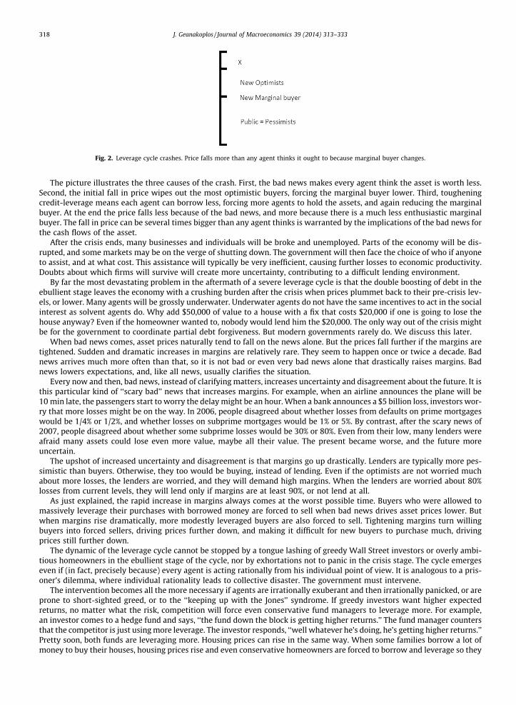
Fig. 2. Leverage cycle crashes. Price falls more than any agent thinks it ought to because marginal buyer changes.


The picture illustrates the three causes of the crash. First, the bad news makes every agent think the asset is worth less.Second, the initial fall in price wipes out the most optimistic buyers, forcing the marginal buyer lower. Third, tougheningcredit-leverage means each agent can borrow less, forcing more agents to hold the assets, and again reducing the marginalbuyer. At the end the price falls less because of the bad news, and more because there is a much less enthusiastic marginalbuyer. The fall in price can be several times bigger than any agent thinks is warranted by the implications of the bad news forthe cash flows of the asset.

After the crisis ends, many businesses and individuals will be broke and unemployed. Parts of the economy will be dis-rupted, and some markets may be on the verge of shutting down. The government will then face the choice of who if anyoneto assist, and at what cost. This assistance will typically be very inefficient, causing further losses to economic productivity.Doubts about which firms will survive will create more uncertainty, contributing to a difficult lending environment.

By far the most devastating problem in the aftermath of a severe leverage cycle is that the double boosting of debt in theebullient stage leaves the economy with a crushing burden after the crisis when prices plummet back to their pre-crisis lev-els, or lower. Many agents will be grossly underwater. Underwater agents do not have the same incentives to act in the socialinterest as solvent agents do. Why add $50,000 of value to a house with a fix that costs $20,000 if one is going to lose thehouse anyway? Even if the homeowner wanted to, nobody would lend him the $20,000. The only way out of the crisis mightbe for the government to coordinate partial debt forgiveness. But modern governments rarely do. We discuss this later.

When bad news comes, asset prices naturally tend to fall on the news alone. But the prices fall further if the margins aretightened. Sudden and dramatic increases in margins are relatively rare. They seem to happen once or twice a decade. Badnews arrives much more often than that, so it is not bad or even very bad news alone that drastically raises margins. Badnews lowers expectations, and, like all news, usually clarifies the situation.

Every now and then, bad news, instead of clarifying matters, increases uncertainty and disagreement about the future. It isthis particular kind of ‘‘scary bad’’ news that increases margins. For example, when an airline announces the plane will be10 min late, the passengers start to worry the delay might be an hour. When a bank announces a $5 billion loss, investors wor-ry that more losses might be on the way. In 2006, people disagreed about whether losses from defaults on prime mortgageswould be 1/4% or 1/2%, and whether losses on subprime mortgages would be 1% or 5%. By contrast, after the scary news of2007, people disagreed about whether some subprime losses would be 30% or 80%. Even from their low, many lenders wereafraid many assets could lose even more value, maybe all their value. The present became worse, and the future moreuncertain.

The upshot of increased uncertainty and disagreement is that margins go up drastically. Lenders are typically more pes-simistic than buyers. Otherwise, they too would be buying, instead of lending. Even if the optimists are not worried muchabout more losses, the lenders are worried, and they will demand high margins. When the lenders are worried about 80%losses from current levels, they will lend only if margins are at least 90%, or not lend at all.

As just explained, the rapid increase in margins always comes at the worst possible time. Buyers who were allowed tomassively leverage their purchases with borrowed money are forced to sell when bad news drives asset prices lower. Butwhen margins rise dramatically, more modestly leveraged buyers are also forced to sell. Tightening margins turn willingbuyers into forced sellers, driving prices further down, and making it difficult for new buyers to purchase much, drivingprices still further down.

The dynamic of the leverage cycle cannot be stopped by a tongue lashing of greedy Wall Street investors or overly ambi-tious homeowners in the ebullient stage of the cycle, nor by exhortations not to panic in the crisis stage. The cycle emergeseven if (in fact, precisely because) every agent is acting rationally from his individual point of view. It is analogous to a pris-oner’s dilemma, where individual rationality leads to collective disaster. The government must intervene.

The intervention becomes all the more necessary if agents are irrationally exuberant and then irrationally panicked, or areprone to short-sighted greed, or to the ‘‘keeping up with the Jones’’ syndrome. If greedy investors want higher expectedreturns, no matter what the risk, competition will force even conservative fund managers to leverage more. For example,an investor comes to a hedge fund and says, ‘‘the fund down the block is getting higher returns.’’ The fund manager countersthat the competitor is just using more leverage. The investor responds, ‘‘well whatever he’s doing, he’s getting higher returns.’’Pretty soon, both funds are leveraging more. Housing prices can rise in the same way. When some families borrow a lot ofmoney to buy their houses, housing prices rise and even conservative homeowners are forced to borrow and leverage so they


too can live in comparable houses, if keeping up with their peers is important to them. At the bottom end, nervous investorsmight withdraw their money, forcing hedge fund managers to sell just when they think the opportunities are greatest. How-ever, of all the irrationalities that exacerbated this leverage cycle, I would not point to these or to homeowners who took outloans they could not really afford, but rather to lenders who underestimated the put option and failed to ask for enoughcollateral.

The aftermath too is an inevitable outcome of a big enough leverage cycle, even if traders were completely rational, pro-cessing information dispassionately. When we add the possibility of panic and the turmoil created by more and more bank-ruptcies, it is not surprising to see lending completely dry up.

The observation that collateral rates are even more important outcomes of supply and demand than interest rates, andeven more in need of regulation, was made over 400 years ago. In The Merchant of Venice, Shakespeare depicted accuratelyhow lending works: one has to negotiate not just an interest rate but the collateral level too. And it is clear which of the twoShakespeare thought was the more important. Who can remember the interest rate Shylock charged Antonio? But everybodyremembers the ‘‘pound of flesh’’ that Shylock and Antonio agreed on as collateral. The upshot of the play, moreover, is thatthe regulatory authority (the court) intervenes and decrees a new collateral level – very different from what Shylock andAntonio had freely contracted – ‘‘a pound of flesh, but not a drop of blood.’’ The Fed, too, could sometimes decree differentcollateral levels (before the fact, not after, as in Shakespeare).

The modern study of collateral seems to have begun with Bernanke et al. (1996, 1999), Kiyotaki and Moore (1997),Holmstrom and Tirole (1997), Geanakoplos (1997, 2003), and Geanakoplos and Zame (2009).14 Bernanke, Gertler, andGilchrist and Holmstrom and Tirole emphasize the asymmetric information between borrowers and lenders as the source oflimits on borrowing. For example, Holmstrom and Tirole argue that the managers of a firm would not be able to borrow allthe inputs necessary to build a project, because lenders would like to see them bear risk, by putting their own money down,to guarantee that they exert maximal effort. Kiyotaki and Moore (1997) and Geanakoplos (1997) study the case where thecollateral is an asset such as a mortgage security, where the buyer/borrower using the asset as collateral has no role in managingthe asset, and asymmetric information is therefore not important. The key difference between Kiyotaki and Moore andGeanakoplos (1997) is that in Kiyotaki and Moore, there is no uncertainty, and so the issue of leverage as a ratio of loan to valuedoes not play a central role; to the extent it does vary, leverage in Kiyotaki and Moore goes in the wrong direction, getting high-er after bad news, and dampening the cycle. In Geanakoplos (1997, 2003), I introduce uncertainty and solve for equilibriumleverage and equilibrium default rates; I show how leverage could be determined by supply and demand, and how under someconditions, volatility (or more precisely, the tail of the asset return distribution) pins down leverage. In Geanakoplos (2003), Iintroduce the leverage cycle in which changes in the volatility of news lead to changes in leverage, which in turn lead to changesin asset prices. At the maximum leverage end of the leverage cycle, asset prices can be much higher than in the correspondingcomplete markets Arrow–Debreu economy, and the drop in prices from peak to trough can be much greater than in the Arrow–Debreu economy. This line of research has been pursued by Gromb and Vayanos (2002), Fostel and Geanakoplos (2008),Brunnermeier and Pedersen (2009), and Adrian and Shin (2010), among others.

5.1. What is so bad about the leverage cycle?

The crisis stage is obviously bad for the economy. But the leverage that brings it on stimulates the economy in good times.Why should we think the bad outweighs the good? After all, we are taught in conventional complete-markets economicsthat the market decides best on these types of trade-offs. In Geanakoplos (2010), I discuss eight reasons why the leveragecycle may nevertheless be bad for the economy. The first three are caused by the large debts and numerous bankruptciesthat occur in big leverage cycles.

First, optimistic investors can impose an externality on the economy if they internalize only their private loss from abankruptcy in calculating how much leverage to take on. For example, managers of a firm calculate their own loss in profitsin the down states, but sometimes neglect to take into their calculations the disruption to the lives of their workers whenthey are laid off in bankruptcy. If, in addition, the bankruptcy of one optimist makes it more likely in the short run that otheroptimists (who are also ignoring externalities) will go bankrupt, perhaps starting a chain of defaults, then the externality canbecome so big that simply curtailing leverage can make everybody better off.

Second, debt overhang destroys productivity, even before bankruptcy, and even in cases when bankruptcy is ultimatelyavoided. Banks and homeowners and others who are underwater often forgo socially efficient and profitable activities. Ahomeowner who is underwater loses much of the incentive to repair a house, even if the cost of the repairs is less thanthe gain in value to the house, since increases in the value of the house will not help him if he thinks he will likely be fore-closed eventually anyway.15

Third, seizing collateral often destroys a significant part of its value in the process. The average foreclosure of a subprimeloan leads to recovery of only 25% of the loan, after all expenses and the destruction of the house are taken into account, as Idiscuss later. Auction sales of foreclosed houses usually bring 30% less than comparable houses sold by their owners.

14 Minsky (1986) was a modern pioneer in calling attention to the dangers of leverage. But to the best of my knowledge, he did not provide a model or formaltheory. Tobin and Golub (1998) devote a few pages to leverage and the beginnings of a model.

15 See Myers (1977) and Gyourko and Saiz (2004).


The next four reasons stem from the swings in asset prices that characterize leverage cycles. A key externality that bor-rowers and lenders in both the mortgage and repo markets do not recognize is that if leverage were curtailed at the high endof the leverage cycle, prices would fall much less in the crisis. Foreclosure losses would then be less, as would inefficienciescaused by agents being so far underwater. One might argue that foreclosure losses and underwater inefficiencies should betaken into account by a rational borrower and lender and be internalized: it may be so important to get the borrower themoney, and the crisis might ex ante be so unlikely, that it is ‘‘second best’’ to go ahead with the big leverage and bearthe cost of the unlikely foreclosure. But that overlooks the pecuniary externality: by going into foreclosure, a borrower low-ers housing prices and makes it more likely that his neighbor will do the same.

Fifth, asset prices can have a profound effect on economic activity. As James Tobin argued with his concept of Q, when theprices of old assets are high, new productive activity, which often involves issuing financial assets that are close substitutesfor the old assets, is stimulated. When asset prices are low, new activity might grind to a halt.16 A large group of small busi-nesspeople who cannot buy insurance against downturns in the leverage cycle can easily sell loans to run their businesses orpay for their consumption in good times at the height of the leverage cycle, but have a hard time at the bottom. Governmentpolicy may well have the goal of protecting these people by smoothing out the leverage cycle.17

Sixth, the large fluctuations in asset prices over the leverage cycle lead to massive redistributions of wealth and changes ininequality. When leverage k = 30, there can be wild swings in returns and losses. In the ebullient stage, the optimists becomerich as their bets pay off, while in the down states, they might go broke. Inequality becomes extreme in both kinds of states.18

Seventh, the leverage cycle is bigger when the heterogeneity of agent valuations of the assets is greater. Very high lever-age means that the asset prices are set by a small group of investors, as Fig. 1 made clear. If agent beliefs are heterogeneous,why should the prices be determined entirely by the highest outliers? In the current crisis, as I observed earlier, the $2.5trillion of toxic mortgage securities were purchased with about $150 billion in cash and $2.35 trillion in loans. As of2006, just two men, Warren Buffet and Bill Gates, between them had almost enough money to purchase every single toxicmortgage security in the whole country. Leverage allows the few to wield great influence on prices and, therefore, on what isproduced. Suppose the heterogeneity is due to differences of opinion, and that the truth is near the middle of the opinions.19

When asset prices are well above the complete-markets price, because of the expectation by the leveraged few that good timesare coming, a huge wave of overbuilding usually results. In the bad state, this overbuilding needs to be dismantled at great costand, more importantly, new building nearly stops.

The eighth problem with the leverage cycle is caused by the inevitable government responses to the crisis stage. In aneffort to mitigate the crisis, the government often intervenes in inefficient ways. In the current crisis, the government is sup-porting the financial sector by holding the federal funds rate near zero. The government’s foreclosure prevention efforts havecreated financial subsidies for households that opt not to move, which can create inefficiencies in labor market adjustment.20

Government bailouts, even if they were all for the public good, cause resentment from those who are not bailed out. The agentsin the economy do not take into account that by leveraging more and putting the economy at greater risk, they create moreinefficient government interventions. And of course, the expectation of being assisted by the government, should things gowrong, causes many agents to be more reckless in the first place.21

6. The leverage cycle of 2000–2009 fits the pattern

6.1. Leverage and prices

By now, it is obvious to everybody that asset prices soared from 1999 (or at least after the disaster period that began Sep-tember 11, 2001) to 2006, and then collapsed from 2007 to 2009. My thesis is that this rise in prices was accompanied bydrastic changes in leverage, and was therefore just part of the 1999–2006 upswing in the leverage cycle after the crisis stagein 1997–1998 at the end of the last leverage cycle. I do not dispute that irrational exuberance and then panic played a role inthe evolution of prices over this period, but I suggest that they may not be as important as leverage; certainly, it is harder toregulate animal spirits than it is leverage.

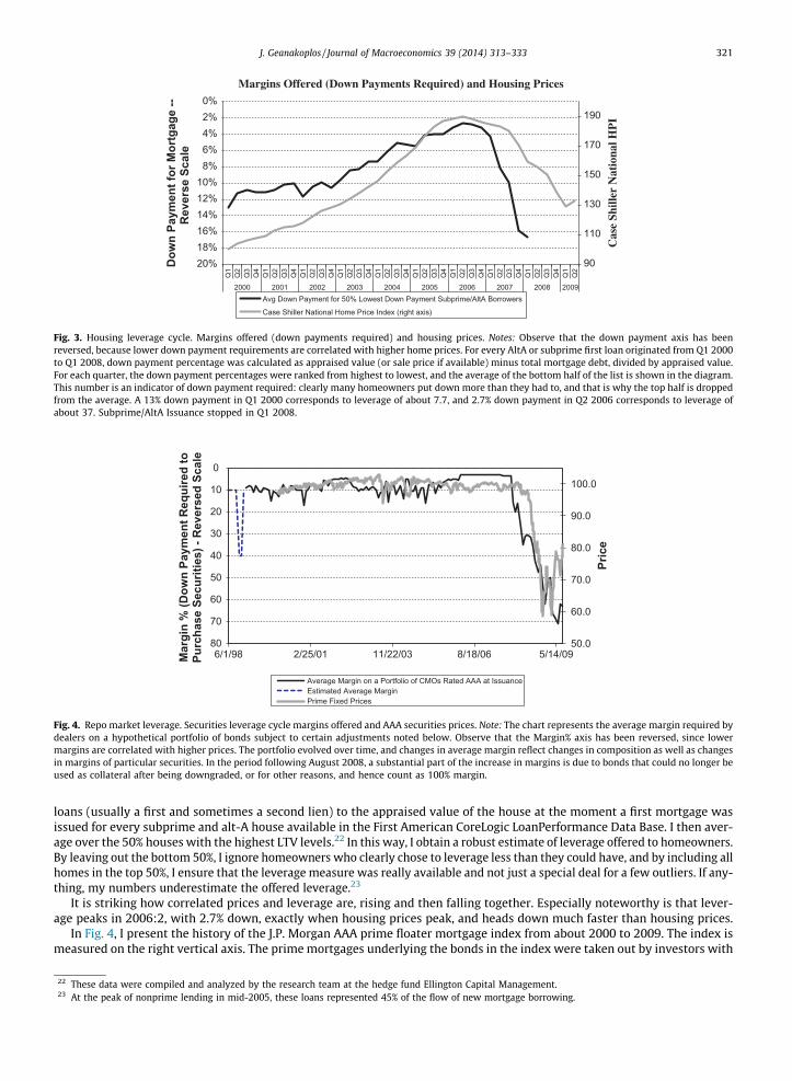
Let us begin with the housing bubble, famously documented by Robert Shiller. In Fig. 3, I display the Case-Shiller nationalhousing index for 2000–2009. It begins at 100 in 2000:1, reaches 190 in 2006:2, and falls to 130 by 2009:1, as measured on theright vertical axis. But I superimpose on that graph a graph of leverage available to homeowners each month. This is measuredon the left vertical axis and labeled ‘‘Down payment for mortgage,’’ which is 100% minus the loan-to-value (LTV) ratio. Tocompute this, I begin by looking house by house each month from 2000–2009 at the ratio of all the outstanding mortgage

16 See Tobin and Golub (1998).17 Here I rely on Tobin’s Q and the absence of insurance markets. The small businessmen cannot insure themselves against the crisis stage of the leverage

cycle. In conventional complete-markets economics, they would be able to buy insurance for any such event. A proof that when insurance markets are missingthere is almost always a government intervention in the existing markets that will make everyone better off was given in Geanakoplos–Polemarchakis (1986).

18 This is a purely paternalistic reason for curtailing leverage.19 Standard economics does not really pay any attention to the case where agents have different beliefs, and median beliefs are closer to the truth than

extreme outliers.20 See Ferreira et al. (2010).21 This mechanism has been formalized in Farhi and Tirole (2009).

50.0

60.0

70.0

80.0

90.0

100.00

10

20

30

40

50

60

70

806/1/98 2/25/01 11/22/03 8/18/06 5/14/09

Pric

e

Mar

gin

% (D

own

Paym

ent R

equi

red

to

Purc

hase

Sec

uriti

es) -

Rev

erse

d Sc

ale

Average Margin on a Portfolio of CMOs Rated AAA at IssuanceEstimated Average MarginPrime Fixed Prices

Fig. 4. Repo market leverage. Securities leverage cycle margins offered and AAA securities prices. Note: The chart represents the average margin required bydealers on a hypothetical portfolio of bonds subject to certain adjustments noted below. Observe that the Margin% axis has been reversed, since lowermargins are correlated with higher prices. The portfolio evolved over time, and changes in average margin reflect changes in composition as well as changesin margins of particular securities. In the period following August 2008, a substantial part of the increase in margins is due to bonds that could no longer beused as collateral after being downgraded, or for other reasons, and hence count as 100% margin.

90

110

130

150

170

1900%2%4%6%8%

10%12%14%16%18%20%

Q1

Q2

Q3

Q4

Q1

Q2

Q3

Q4

Q1

Q2

Q3

Q4

Q1

Q2

Q3

Q4

Q1

Q2

Q3

Q4

Q1

Q2

Q3

Q4

Q1

Q2

Q3

Q4

Q1

Q2

Q3

Q4

Q1

Q2

Q3

Q4

Q1

Q2

2000 2001 2002 2003 2004 2005 2006 2007 2008 2009

Cas

e Sh

iller

Nat

iona

l HP

I

Dow

n Pa

ymen

t for

Mor

tgag

e --

Rev

erse

Sca

le

Avg Down Payment for 50% Lowest Down Payment Subprime/AltA Borrowers

Case Shiller National Home Price Index (right axis)

Margins Offered (Down Payments Required) and Housing Prices

Fig. 3. Housing leverage cycle. Margins offered (down payments required) and housing prices. Notes: Observe that the down payment axis has beenreversed, because lower down payment requirements are correlated with higher home prices. For every AltA or subprime first loan originated from Q1 2000to Q1 2008, down payment percentage was calculated as appraised value (or sale price if available) minus total mortgage debt, divided by appraised value.For each quarter, the down payment percentages were ranked from highest to lowest, and the average of the bottom half of the list is shown in the diagram.This number is an indicator of down payment required: clearly many homeowners put down more than they had to, and that is why the top half is droppedfrom the average. A 13% down payment in Q1 2000 corresponds to leverage of about 7.7, and 2.7% down payment in Q2 2006 corresponds to leverage ofabout 37. Subprime/AltA Issuance stopped in Q1 2008.


loans (usually a first and sometimes a second lien) to the appraised value of the house at the moment a first mortgage wasissued for every subprime and alt-A house available in the First American CoreLogic LoanPerformance Data Base. I then aver-age over the 50% houses with the highest LTV levels.22 In this way, I obtain a robust estimate of leverage offered to homeowners.By leaving out the bottom 50%, I ignore homeowners who clearly chose to leverage less than they could have, and by including allhomes in the top 50%, I ensure that the leverage measure was really available and not just a special deal for a few outliers. If any-thing, my numbers underestimate the offered leverage.23

It is striking how correlated prices and leverage are, rising and then falling together. Especially noteworthy is that lever-age peaks in 2006:2, with 2.7% down, exactly when housing prices peak, and heads down much faster than housing prices.

In Fig. 4, I present the history of the J.P. Morgan AAA prime floater mortgage index from about 2000 to 2009. The index ismeasured on the right vertical axis. The prime mortgages underlying the bonds in the index were taken out by investors with

22 These data were compiled and analyzed by the research team at the hedge fund Ellington Capital Management.23 At the peak of nonprime lending in mid-2005, these loans represented 45% of the flow of new mortgage borrowing.

Fig. 5. VIX index.


pristine credit ratings, and the bonds are also protected by some equity in their deals. For most of its history, this index staysnear 100, but starting in early 2008, it falls rapidly, plummeting to 60 in early 2009. The cumulative losses on these primeloans even today, are still in the single digits; it is hard to imagine them ever reaching 40% (which would mean somethinglike 80% foreclosures with only 50% recoveries). It is of course impossible to know what people were thinking about potentialfuture losses when the index fell to 60 in late 2008 and early 2009. My hypothesis is that leverage played a big role in theprice collapse.

On the left vertical axis of Fig. 4, I give the loan-to-value, or, equivalently, the down payment or margin, offered by WallStreet banks to the hedge fund Ellington Capital Management on a changing portfolio of AAA mortgage bonds.24 The Fed didnot keep such historical data; fortunately, the hedge fund Ellington, which I have worked with for the past twenty years, doeskeep its own data. The data set is partly limited in value by the fact that the data were only kept for bonds Ellington actuallyfollowed, and these changed over time. Some of the variation in average margin is due to the changing portfolio of bonds, andnot to changes in leverage. But the numbers, while not perfect, provide substantial evidence for my hypothesis and tell a fas-cinating story. In the 1997–1998 emerging markets/mortgage crisis, margins shot up, but quickly returned to their previous lev-els. Just as housing leverage picked up over the period after 1999, so did security level leverage. Then in 2007, leveragedramatically fell, falling further in 2008, and leading the drop in security prices. Very recently, leverage has started to increaseagain, and so have prices.

Fig. 5 displays the history of implied volatility for the S&P 500, called the VIX index. Volatility in equities is by no means aperfect proxy for volatility in the mortgage market, but it is striking that the VIX reached its peak in 2008 at the crisis stage ofthe current leverage cycle, and reached a local peak in 1998 at the bottom of the last leverage cycle in fixed-income secu-rities. The VIX also shot up in 2002, but there is no indication of a corresponding drop in leverage in the Ellington mortgagedata.

6.2. Leverage and prices world wide

The pattern we just saw in America was repeated across the global stage. Consider a study done at the San Francisco Fedon the correlation between changes from 1997 to 2007 in household leverage (defined as debt to income) and housing pricesfor 16 countries (Glick and Lansing, 2010).

One can see in Fig. 6 that for many countries, like Ireland and Spain and Portugal, household leverage soared, whereas forother countries like Japan and Germany household leverage actually dropped slightly. Fig. 7 makes it clear that in countrieswhere household leverage increased, housing prices increased.

The last figure (Fig. 8) from the San Francisco Fed shows that the drop in income after the crash was also worst in coun-tries where household leverage and housing prices had increased the most.

Similarly results for household leverage and drops in consumption across different zip codes in the United States werefound by Mian and Sufi (2010), displayed in Fig. 9.

6.3. What triggered the crisis?

The subprime mortgage security price index collapsed in February 2007. The stock market kept rising until October 2007,when it too started to fall, losing eventually around 57% of its value by March 2009 before rebounding to within 27% or so of

24 These are the offered margins and do not reflect the leverage chosen by Ellington, which since 1998 has been drastically smaller than what was offered.

Fig. 7. Household leverage and the run-up in house-prices. Notes: Leverage is debt to equity in this study. The plotted line depicts the best fit relationship inthe data as generated by a simple least square statistical regression. Source: Federal Reserve Bank San Francisco, Glick-Lansing FRBSF 2010.

Fig. 8. Household leverage and the decline in consumption. Note: The plotted line depicts the best fit relationship in the data as generated by a simple leastsquare statistical regression. Source: Federal Reserve Bank San Francisco, Glick-Lansing FRBSF 2010.

Fig. 6. Household leverage ratios: debt to disposable income. Note: The following countries use different data years: Japan 1997, 2006; Spain 2000, 2007;Ireland 2002, 2007. Source: Federal Reserve Bank San Francisco, Glick-Lansing FRBSF 2010.


its October peak in January 2010. What, you might wonder, was the cataclysmic event that set prices and leverage on theirdownward spiral?

The point of my theory is that when an economy is highly leveraged, the fall in prices from scary bad news is naturallygoing to be out of proportion to the significance of the news, because the scary bad news precipitates and feeds a plunge in

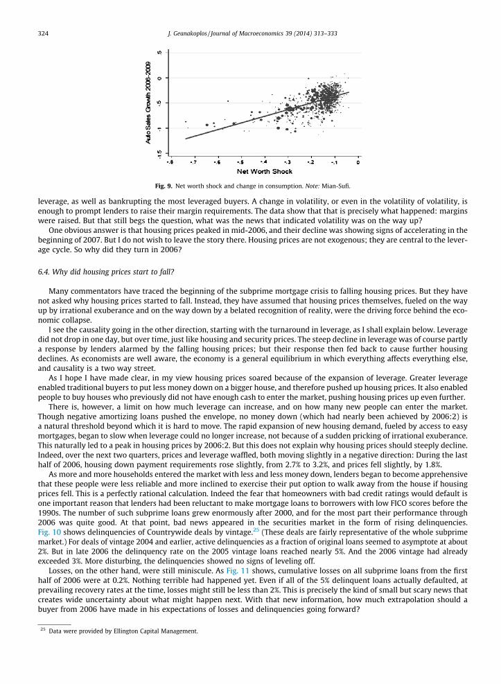
Fig. 9. Net worth shock and change in consumption. Note: Mian-Sufi.


leverage, as well as bankrupting the most leveraged buyers. A change in volatility, or even in the volatility of volatility, isenough to prompt lenders to raise their margin requirements. The data show that that is precisely what happened: marginswere raised. But that still begs the question, what was the news that indicated volatility was on the way up?

One obvious answer is that housing prices peaked in mid-2006, and their decline was showing signs of accelerating in thebeginning of 2007. But I do not wish to leave the story there. Housing prices are not exogenous; they are central to the lever-age cycle. So why did they turn in 2006?

6.4. Why did housing prices start to fall?

Many commentators have traced the beginning of the subprime mortgage crisis to falling housing prices. But they havenot asked why housing prices started to fall. Instead, they have assumed that housing prices themselves, fueled on the wayup by irrational exuberance and on the way down by a belated recognition of reality, were the driving force behind the eco-nomic collapse.

I see the causality going in the other direction, starting with the turnaround in leverage, as I shall explain below. Leveragedid not drop in one day, but over time, just like housing and security prices. The steep decline in leverage was of course partlya response by lenders alarmed by the falling housing prices; but their response then fed back to cause further housingdeclines. As economists are well aware, the economy is a general equilibrium in which everything affects everything else,and causality is a two way street.

As I hope I have made clear, in my view housing prices soared because of the expansion of leverage. Greater leverageenabled traditional buyers to put less money down on a bigger house, and therefore pushed up housing prices. It also enabledpeople to buy houses who previously did not have enough cash to enter the market, pushing housing prices up even further.

There is, however, a limit on how much leverage can increase, and on how many new people can enter the market.Though negative amortizing loans pushed the envelope, no money down (which had nearly been achieved by 2006:2) isa natural threshold beyond which it is hard to move. The rapid expansion of new housing demand, fueled by access to easymortgages, began to slow when leverage could no longer increase, not because of a sudden pricking of irrational exuberance.This naturally led to a peak in housing prices by 2006:2. But this does not explain why housing prices should steeply decline.Indeed, over the next two quarters, prices and leverage waffled, both moving slightly in a negative direction: During the lasthalf of 2006, housing down payment requirements rose slightly, from 2.7% to 3.2%, and prices fell slightly, by 1.8%.

As more and more households entered the market with less and less money down, lenders began to become apprehensivethat these people were less reliable and more inclined to exercise their put option to walk away from the house if housingprices fell. This is a perfectly rational calculation. Indeed the fear that homeowners with bad credit ratings would default isone important reason that lenders had been reluctant to make mortgage loans to borrowers with low FICO scores before the1990s. The number of such subprime loans grew enormously after 2000, and for the most part their performance through2006 was quite good. At that point, bad news appeared in the securities market in the form of rising delinquencies.Fig. 10 shows delinquencies of Countrywide deals by vintage.25 (These deals are fairly representative of the whole subprimemarket.) For deals of vintage 2004 and earlier, active delinquencies as a fraction of original loans seemed to asymptote at about2%. But in late 2006 the delinquency rate on the 2005 vintage loans reached nearly 5%. And the 2006 vintage had alreadyexceeded 3%. More disturbing, the delinquencies showed no signs of leveling off.

Losses, on the other hand, were still miniscule. As Fig. 11 shows, cumulative losses on all subprime loans from the firsthalf of 2006 were at 0.2%. Nothing terrible had happened yet. Even if all of the 5% delinquent loans actually defaulted, atprevailing recovery rates at the time, losses might still be less than 2%. This is precisely the kind of small but scary news thatcreates wide uncertainty about what might happen next. With that new information, how much extrapolation should abuyer from 2006 have made in his expectations of losses and delinquencies going forward?

25 Data were provided by Ellington Capital Management.

Fig. 11. ABX.HE cumulative loss by reporting month (% of original balance).

Fig. 10. DQ/Orig (Scary Bad News).


The ABX index for 2006 vintage subprime bonds began to fall in November 2006 with the smallest trickle of bad newsabout homeowner delinquencies, then spiked downward in January 2007 after the year-end delinquency report (Fig. 12).This price drop of 2006 BBB bonds to below 80 implied that the market was suddenly anticipating huge losses on subprimedeals on the order of 9%. (The BBB tranche absorbs the first losses after the overcollateralization.) Recall that for a pool ofmortgages to lose 9% of its value, the market must anticipate that something like 30% of the homeowners will be thrownout of their houses, with 30% losses on the mortgage on each home sold (30% � 30% = 9%). This expectation turned out tobe not pessimistic enough, but at that time it was a heroic extrapolation from the observed delinquencies of less than 5%.26

In February 2007, after the dramatic fall in BBB subprime mortgage prices, housing prices were still only 1.8% off theirpeak. Though the peak of the housing market preceded the peak of the securities market, the collapse in securities pricespreceded the significant fall in housing prices. Thus, in my view the trigger for the downturn in bonds was the bad newsabout delinquencies, which then spilled over into the housing market.

The downward pressure on bond prices from worrisome delinquency numbers meant that new subprime securitizationsbecame more difficult to underwrite. Securitizers of new loans looked for better loans to package in order to continue to backbonds worth more than the loan amounts they had to give homeowners. They asked for loans with more collateral. As Fig. 3shows, from 2006:4 to 2007:4, the required down payment on houses rose dramatically from 3.2% to 15.9% (equivalently,LTV fell from 96.8% to 84.1%). This meant that potential new homeowners began to be closed out of the market, which ofcourse reduced home prices. In that same period, housing prices began to fall rapidly, declining by 8.5%.

But more insidiously, the desire by lenders to have more collateral for each dollar loaned kept homeowners from refi-nancing because they simply did not have the cash: given the drop in the permissible LTV ratio, and the fall in housing prices,they suddenly needed to put down 25% of their original loan in cash to refinance. Refinancing virtually stopped overnight.Until 2007, subprime bondholders could count on 70% or so of subprime borrowers refinancing by the end of their thirdyear.27 These homeowners began in pools that paid a very high rate of interest because of their low credit rating. But after

26 The collapse of the ABX index in January 2007 is a powerful illustration of the potency of market prices to convey information. This first market crashshould have been enough to alert the American government to the looming foreclosure disaster, but years later the government still has not taken decisiveaction to mitigate foreclosures.

27 Seventy-four percent of all subprime loans issued in or before 2004 had refinanced by the end of their third year, according to the First American CoreLogicLoanPerformance Data Base.

Fig. 12. BBB prices crash before big drop in housing.

Fig. 13. Volume of credit default swaps. Source: ISDA Market Survey: Historical Data


two years of reliable mortgage payments, they would become eligible for new loans at better rates, which they traditionallytook in vast numbers. Of course, a prepayment means a full payment to the bondholder. Once refinancing plummeted and thissure source of cash disappeared, the bonds became much more at risk and their prices fell more. Margins on subprime bondsbegan to tighten.

Mortgagees who had anticipated being able to refinance were trapped in their original loans at high rates; many subse-quently became delinquent and entered foreclosure. Foreclosures obviously lead to forced sales and downward pressure onhousing prices. And falling home prices are a powerful force for further price reductions, because when house values fall belowthe loan amount, homeowners lose the incentive to repay their loans, leading to more defaults, foreclosures, and forced selling.All this leads back to falling security prices and tighter margins on securities, including prime securities, as we saw in Fig. 4.28

The feedback from falling security prices to higher margins on housing loans to lower house prices and then back totougher margins on securities and to lower security prices and then back again to housing is what I call ‘‘the double leveragecycle.’’

My purpose here was to explain what made downpayments shoot up for homeowners. I argued it was caused by the col-lapse of the subprime mortgage securities market after the bad delinquency reports at the end of 2006. But I cannot resistmentioning my contention that this sudden drop in subprime security prices, and the further price declines later, were notsimply the result of a drop in expected payoffs (that is, in fundamentals) by the same old buyers, but also the result of achange in the marginal buyer. The bad news and the tightening margins story applies to the security markets just as it doesto the housing market. But for mortgage securities a critical new downward force entered the market. Standardized creditdefault swaps (CDS) on mortgage bonds were created for the first time in late 2005, at the very height of the market. Thevolume of CDS expanded rapidly throughout 2006 and especially in 2007 (Fig. 13).29 A CDS is an insurance contract for a bond.

28 In the case of subprime securities, the fall in security prices preceded the tightening of margins. But as Fig. 4 seems to show, for securities of primemortgages, the tightening of margins came before the fall in security prices.

29 Chart 7 is derived from data provided in ‘‘ISDA Market Survey: Historical Data,’’ available at www.isda.org/statistics/historical/html. Unfortunately, itincludes all CDS, not just CDS on mortgages. The data on mortgage CDS seem difficult to find, since these CDS were traded bilaterally and not on an exchange. Itseems very likely to me that the mortgage CDS increased even more dramatically from 2004–2005 to 2006–2007.

http://www.isda.org/statistics/historical/html


By buying the insurance, the pessimists for the first time could leverage their negative views about bond prices and the housesthat backed them. Instead of sitting out of the subprime securities market, pessimists could actively push bond prices down.Their purchase of insurance is tantamount to the creation of more (‘‘synthetic’’) bonds; naturally, the increase in supply pushedthe marginal buyer down and thus the price down.

6.5. Why was this leverage cycle so bad?

The leverage cycle has recurred many times in the United States and abroad. I have mentioned the 1994 Treasury crashand the 1997–1998 emerging markets and mortgage crash as two examples that preceded the 2007–2009 crash in mort-gages in the United States. The land boom and bust in Japan in 1990 is another one. I would like to briefly give four reasonswhy this latest leverage cycle in the United States has been the worst since the Great Depression.30 First, leverage got higherthan it ever had before, in housing and in securities. Part of that is simply that margins went down in the great moderation asvolatility stayed low, as we have discussed, and another part is the tranching that securitization made possible, which is a moresophisticated kind of leverage. As I mentioned, if markets are calm, financial innovation will always tend to increase leverage.Second, there was a double leverage cycle, because the housing market and the mortgage securities market affect each other;trouble in either one brings down the other. Third, the aftermath of the crisis was extended because so many homeowners andbusinesses were under water (and the government did so little to help them). Lastly, the introduction of CDS, at the moment thesecurities market was its highest and most leveraged, was new.

7. What should have been done and what should we do?

Economists and the Federal Reserve ask themselves every day whether the economy is picking the right interest rates. Butone can also ask the question whether the economy is picking the right equilibrium margins. At both ends of the leveragecycle, it does not do so. In ebullient times, the equilibrium collateral rate is too loose; that is, equilibrium leverage is too high.In bad times, equilibrium leverage is too low. As a result, in ebullient times asset prices are too high, and in crisis times theyplummet too low. This is the leverage cycle.

7.1. Before a crisis?

The policy implication of the leverage cycle is that the Fed should manage system wide leverage, seeking to maintain itwithin reasonable limits in normal times, stepping in to curtail it in times of ebullience, and propping it up as market actorsbecome anxious, and especially in a crisis. To carry out this task, of course, the Fed must first monitor leverage. The Fed mustcollect data from a broad spectrum of lenders and investors. This should include all bank household lending and repo lend-ing, as well as borrowing data from hitherto secretive hedge funds, on how much leverage is being used to buy various clas-ses of assets. Moreover, the amount of leverage being employed must be transparent. The accounting and legal rules thatgovern devices, such as structured investment vehicles, that were used to mask leverage levels must be reformed to ensurethat leverage levels can be more readily and reliably discerned by the market and regulators alike. The best way to monitorleverage is to do it at the security level by keeping track of haircuts on all the different kinds of assets used as collateral,including in the repo market and in the housing market. Also very useful, but less important, is monitoring the investor lever-age (or the debt-equity ratio) of big firms.

In my opinion, the crisis has shown us most emphatically that monitoring the whole credit surface is absolutely a toppriority. To the best of my knowledge, the central banks of America and Europe have taken half hearted steps to obtain thisinformation. There are now questionnaires that must be filled out by various investors, but the questions are vague. They ask,what is the average LTV on the securities you have on repo? What I would like to see is the collection of data on every singleloan to or from any systemically important financial institution (SIFI). At one point the Office of Financial Research (OFR) wasmeant to acquire precisely this kind of information. From such data, the credit surface could be mapped out. I am not awarethat this mandate is being carried out. If such detailed information is being acquired, it certainly has not been disseminated.

Collecting the information is just the first step. The next step is to oblige the central bank to target the whole credit sur-face, not just the riskless interest rates. At first that might mean acting directly to set riskless interest rates (by making loansavailable to a few chosen banks for which there is a reasonable expectation of full repayment), but predicting the effect onthe rest of the credit surface. But I believe the crisis has shown us that the Fed and other central banks must then be willingto set limits to leverage, or more generally, via taxation or other interventions, ensure that interest rates are high when lever-age is high. Central banks need to intervene directly over larger parts of the credit surface.

It is often asked, how would the Fed know when leverage was getting too high? Perhaps borrowers with improved riskmanagement techniques are able to manage higher leverage? The answer is that if leverage is moving substantially higherthan it has in the past, on the same collateral, and if in addition the collateral is rising rapidly in price, then it is likely lever-age has gotten too high and must be reined in. If LTVs on houses goes from an average of 86% to 97%, while housing prices are

30 In Geanakoplos (2012) I give nine reasons.


soaring, the Fed should intervene and limit the loans that banks can make, as the Bank of Israel did in 2010. This the what theFed and the ECB failed to do, and are reluctant to consider doing in the future.

The Fed already had two goals, of maintaining low inflation and low unemployment, and essentially just one instrument.Now it must worry about financial stability as well. It is clear that it needs more instruments to do its job.

7.2. During the crisis?

In the crisis of late 2008–2009, the first order of business was to stop the panic, and forestall bank runs or money marketruns. Here the Federal Reserve and the US Treasury behaved splendidly. No small part in their success was played byprograms like TALF, which propped up leverage by enabling the Fed to make direct loans to investors at interest rates thatprivate lenders would offer only with much more collateral. Thus the Fed offered 95% LTV loans at near riskless interest ratesagainst credit card securities, automobile securities, and tuition securities. In other words, it acted directly on risky parts ofthe credit surface. The facilities the Fed set up to administer these extraordinary loans have been dismantled. This is amistake. How can we be sure there will not be another crisis? And why should we not avail ourselves of the facilities beforewe are plunged into the depths of the next crisis?

7.3. After a crisis?

7.3.1. Debt forgivenessThe American crisis began almost seven years ago in February 2007 when the BBB subprime index collapsed. The econ-

omy is finally starting to pick up, but unemployment is still over 7%, down from its high of over 10%. We are often told thatthings could have been much worse. I believe they could also have been much better.

Our biggest mistake after the crisis began was not taking effective measures to ameliorate the massive foreclosure prob-lem, or to confront the problems of debt overhang for homeowners, small businesses, and government. We did save ourbanks. What we should have done is partially forgive subprime debt.

Over 4 million homes were foreclosed as a result of the American mortgage crisis, and counting all the loans that aredelinquent or underwater and potentially headed for default, the number may reach 7 million. At an average of 3 peopleper household, that is 20 million people thrown out of their homes for defaulting, double the number of people in Greece.

In a New York Times op-ed with Susan Koniak (Geanakoplos and Koniak, 2008) I warned of the impending foreclosuredisaster, and predicted that government efforts to help homeowners by temporarily reducing their interest payments wouldfail. We argued that subprime borrowers, without a good credit rating to protect, who were far underwater and who took ahit in their earnings would default. We had evidence already coming in that they were defaulting, and sure enough they diddefault in huge numbers. Fig. 14, which we included in a subsequent New York Times op-ed a few months later, shows themonthly rate of new defaults for various kinds of mortgages, with subprime mortgages at the top. For subprime loans withLTV of 140% to 160%, the rate of new defaults was 7.4% per month!

In another NY Times op-ed (Geanakoplos and Koniak, 2009), Susan Koniak and I advocated reducing principal as the onlyway to help homeowners and lenders and the country at the same time. Losses from foreclosures of subprime loans havebeen horrible. The average recovery is under 25%. This is understandable once one realizes that in many states it takes18 month to three years to throw somebody out of his house. In that time the mortgage isn’t paid, the taxes aren’t paid,the house is not repaired, the house is often vandalized, and the realtor must be paid. Consider a $160,000 subprime loanon a house that is now worth only $100,000. If the borrower loses his job or finds his earnings prospects are reduced, he willdefault. The lender will then end up with about $40,000. But if the loan is forgiven down to $90,000 (perhaps with the addedproviso that if the house rises in value and is then sold, half the sale price beyond $100,000 will also be returned to the len-der), both the lender and the borrower can be made better off. The borrower might choose to stay in his house and continueto pay the mortgage, or he might decide to sell the house as expeditiously as possible, returning $90,000 to the lender andpocketing the $10,000 himself. Either way the lender makes out much better than with $40,000.

Fig. 14. Net monthly flow (excluding mods) from <60 days to P60 days DQ (6 month average as of January 09).

0% 10% 20% 30% 40% 50% 60% 70% 80% 90%

1 2 3 4 5 6 7 8 9 10 11 12 13 14 15 16 17 18

Cum

ulat

ive

Rec

idiv

ism

Months Since Mod

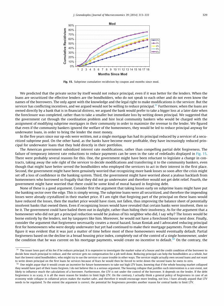
Mod

2%3%4%5%6%

Fig. 15. Subprime cumulative recidivism by coupon and months since mod.


We predicted that the private sector by itself would not reduce principal, even if it was better for the lenders. When theloans are securitized the effective lenders are the bondholders, who do not speak to each other and do not even know thenames of the borrowers. The only agent with the knowledge and the legal right to make modifications is the servicer. But theservicer has conflicting incentives, and we argued would not be willing to reduce principal.31 Furthermore, when the loans areowned directly by a bank that is in financial distress, we argued the bank would prefer to take a bigger loss at a later date whenthe foreclosure was completed, rather than to take a smaller but immediate loss by writing down principal. We suggested thatthe government cut through the coordination problem and hire local community bankers who would be charged with theassignment of modifying subprime mortgages in their community in order to maximize the revenue to the lender. We figuredthat even if the community bankers ignored the welfare of the homeowners, they would be led to reduce principal anyway forunderwater loans, in order to bring the lender the most money.

In the five years since our op-eds were written, not a single mortgage has had its principal reduced by a servicer of a secu-ritized subprime pool. On the other hand, as the banks have become more profitable, they have increasingly reduced prin-cipal for underwater loans that they hold directly in their portfolios.

The American government subsidized interest rate modifications, rather than compelling partial debt forgiveness. Thefailure of temporary interest rate reductions to reduce payments can be seen in the rate of redefaults displayed in Fig. 15.There were probably several reasons for this. One, the government might have been reluctant to legislate a change in con-tracts, taking away the sole right of the servicer to decide modifications and transferring it to the community bankers, eventhough that might have better served the bondholders who employed the servicers to act in their interest in the first place.Second, the government might have been genuinely worried that recognizing more bank losses so soon after the crisis mightset off a loss of confidence in the banking system. Third, the government might have worried about a jealous backlash fromhomeowners who borrowed so frugally that they did not go underwater and therefore would not get debt relief. Fourth, thegovernment might have worried that there could be some kind of moral hazard in forgiving debt.

None of these is a good argument. Consider first the argument that taking losses early on subprime loans might have putthe banking sector over the edge. This is simply wrong. The subprime loans were all securitized, and therefore the impendinglosses were already crystallized in their market price. If I am right that forgiving part of the principal on these loans wouldhave reduced the losses, then the market price would have risen, not fallen, thus improving the balance sheet of potentiallyinsolvent banks that owned them. Even if recognizing losses would have revealed that certain banks were insolvent, then sobe it. The government could have bailed them out in daylight, rather than hiding their insolvency. As for the argument that ahomeowner who did not get a principal reduction would be jealous of his neighbor who did, I say why? The losses would beborne entirely by the lenders, not by taxpayers like him. Moreover, he would not have a foreclosed house next door. Finally,consider the argument that forgiveness necessarily creates a moral hazard. Susan Koniak and I advocated reducing principalfirst for homeowners who were deeply underwater but yet had continued to make their mortgage payments. From the abovefigure it was evident that it was just a matter of time before most of these homeowners would eventually default. Partialforgiveness based on the decline in a broad housing price index, completely out of the control of a single homeowner, underthe condition that he was current on his mortgage payments, would create no incentive to default.32 On the contrary, the

31 The issuer loses part of his fee if he reduces principal. It is expensive to investigate the market value of a house and the credit condition of the borrower todecide how much principal to reduce, and the servicer gets no compensation for a job well done. Reducing principal can help the bondholders as a whole, buthurt the lowest rated bondholders, who might try to sue the servicer or cause trouble in other ways. The servicer might actually own second loans and not wantto write down principal on the first loans he services because of fears he would then be forced to write down the second loans he owns to zero.

32 One might argue that it would create an incentive for future homeowners to take out high LTV loans, knowing that if the whole housing market collapsedthey would have part of their loans forgiven. I do not believe this is a serious argument. The housing collapse that justifies such intervention is a rare event, notlikely to influence much the calculations of a borrower. Furthermore, the LTV is not under the control of the borrower. It depends on the lender. If the debtforgiveness is so scary, it is all the more reason for lenders to limit high LTV. On the contrary, I actually think a general policy of forgiveness in case of aneconomy wide collapse in collateral prices makes the market safer, and therefore it would encourage more lending, not less. I have already argued that LTVneeds to be regulated. To the extent the argument is correct, the potential for forgiveness provides another reason for central banks to limit LTV.


policy adopted by the Obama administration, to give relief in the form of (sometimes temporary) interest rate reductions afterthe homeowner had shown his need by defaulting definitely does create a moral hazard, encouraging default.

The nature of promises and debt has been a preoccupation of philosophers for thousands of years. Keeping promises wasPlato’s first proposed definition of justice in the Republic (it was shown not to be always just). Nietzsche, in the Genealogy ofMorals, says the emergence of Conscience came from the repeated punishing of people who failed to honor their debts andthe subsequent internalization of that punishment. (Thus ‘‘schuld’’ is the root of the German word for debt and also for oneversion of Conscience.) As a result people feel it is morally wrong to break a promise, and they take satisfaction in seeing apromise breaker punished, even if it is costly for them to administer the punishment. This appears to me an interestingexplanation for why it is so hard to forgive, even when it is in our own interest.

The subtlest literary analysis of keeping promises can be found in Shakespeare’s Merchant of Venice. The theme of defaultand forgiveness is repeated several times in the play with the story of the rings. When Antonio’s boats have apparently sunk,and a trial is being held to determine if Shylock can obtain his collateral pound of flesh, Portia disguises herself as the judge.Portia is the beautiful and rich woman Bassanio was able to woo and wed with the 3000 ducats Antonio had borrowed fromShylock. Portia and her assistant gave Bassanio and his assistant their rings in exchange for the promise that they wouldnever be taken off their fingers. Shylock has earlier made it clear that he would never break his promise about the ringhis wife Leah gave him. After the verdict, in which Portia the judge rules that Shylock can have his pound of flesh, butnot a drop of blood, Bassanio rushes to congratulate the judge he does not recognize for his wonderful ruling and offers areward of his choosing. She says what about that ring you are wearing. At first Bassanio refuses, but the judge insists. Con-fronted with an urgent and completely unexpected need, Bassanio and his assistant break their promise and give up theirrings. They expect forgiveness. And they get it. ‘‘To do a great right, do a little wrong’’ is Bassanio’s philosophy. Or as Portiadescribes forgiveness of debts, ‘‘The quality of mercy is not strain’d;. . . It blesseth him that gives and him that takes.’’

7.4. Europe

Europe has also had a leverage cycle boom and bust. So did Iceland. As we have mentioned earlier, in Ireland, England,Spain, Portugal, and Denmark a huge expansion in household debt and leverage led to an enormous rise in housing prices.In Greece the government enormously increased borrowing, as the banks did in Iceland. When the bubble burst, each ofthese countries was left with enormous debt relative to its GDP, and in every country it became enormously harder for smallinvestors to get new loans. In Greece and Spain, unemployment is now well over 25% for the population as a whole, and over50% for the young. Rather than debt forgiveness, there has been austerity.

In Greece, after a mighty struggle, the government has managed to reduce the primary deficit to a tiny surplus. But ofcourse that means the Greeks are still unable to service their outstanding debt. The Troika continues to lend Greece moremoney to pay the interest on the old debt, adding the new loans to the debt burden of the country. Together with the shrink-ing GDP and prices, this policy has led to a debt to GDP ratio for Greece of about 160%. It is hard to find a single citizen inGreece or Germany who believes that Greece will actually repay in full, but the Troika continues to maintain the charade thatthe debt can and will be honored. The Greek public is outraged that the country is being crushed under austerity programsthat will in the end fail to enable Greece to repay, and the German public is outraged that its government is throwing goodmoney after bad, lending the Greeks still more money when they know the old debt will not be repaid.

The Troika has apparently calculated that allowing default in Greece is too dangerous. And a slim majority of the Greekpopulation has calculated that it is better to have the guiding hand of the Troika rather than face the uncertainties of default.But eventual default seems a near certainty. The way things are going, under the best of all possible worlds, the debt willeventually be extended, at lower interest rates, and all the parties will ignore the fact that the restructured debt has a muchlower present value than the original debt, which is a tantamount to a partial default or forgiveness.

The Troika did help coordinate the write down of privately held Greek debt. But since the vast majority of the outstandingdebt was held by the official sector, this has not been nearly enough.

Think of how much better it would have been if the Troika had been able to offer debt forgiveness in exchange forreforms. Reform tax collection, and so much of the national debt will be forgiven. Tear down the barriers to entry in variousprofessions, and more debt will be forgiven. Reform the court system and the education system, and still more debt will beforgiven. A deal like that would give the Greeks a chance and the incentive to redeem themselves, and likely recover moremoney for the Troika than the current path. The German public can understand that getting repaid half is better than a Greekcollapse in which Germany does not get paid at all. And the Greek public might get behind the reforms if they thought theywould happen, and that once they happened, Greece would be viable.

8. What we did get afterward: Austerity and quantitative easing

8.1. Austerity

Instead of forgiveness we got austerity. Many economists have criticized the austerity programs going on in the UnitedStates and Europe. Keynes already eloquently argued against the dangers of austerity, showing that it could be self defeating.I would like to add just one thought. Infrastructure is badly needed in some countries like the United States. A necessary

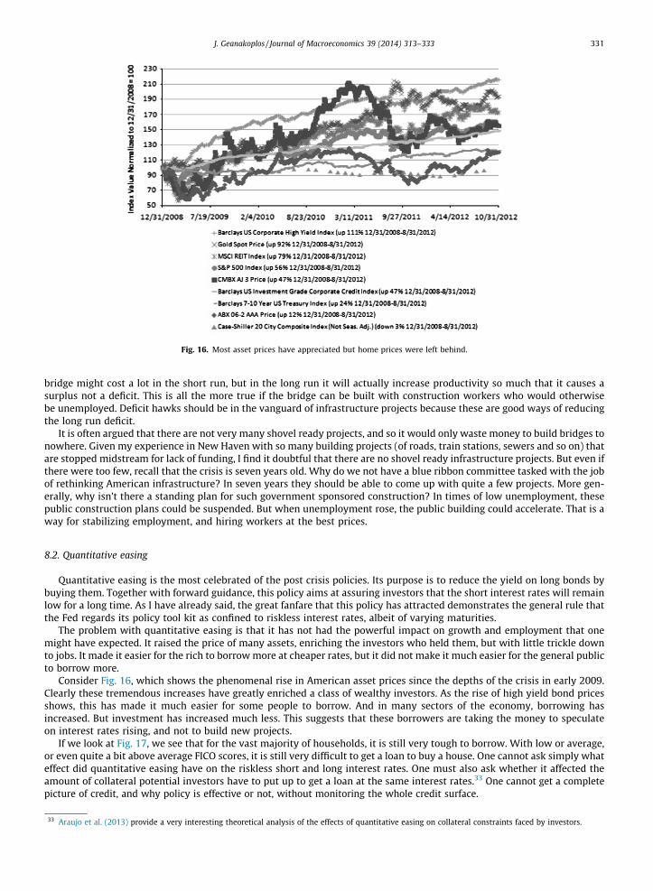
Fig. 16. Most asset prices have appreciated but home prices were left behind.


bridge might cost a lot in the short run, but in the long run it will actually increase productivity so much that it causes asurplus not a deficit. This is all the more true if the bridge can be built with construction workers who would otherwisebe unemployed. Deficit hawks should be in the vanguard of infrastructure projects because these are good ways of reducingthe long run deficit.

It is often argued that there are not very many shovel ready projects, and so it would only waste money to build bridges tonowhere. Given my experience in New Haven with so many building projects (of roads, train stations, sewers and so on) thatare stopped midstream for lack of funding, I find it doubtful that there are no shovel ready infrastructure projects. But even ifthere were too few, recall that the crisis is seven years old. Why do we not have a blue ribbon committee tasked with the jobof rethinking American infrastructure? In seven years they should be able to come up with quite a few projects. More gen-erally, why isn’t there a standing plan for such government sponsored construction? In times of low unemployment, thesepublic construction plans could be suspended. But when unemployment rose, the public building could accelerate. That is away for stabilizing employment, and hiring workers at the best prices.

8.2. Quantitative easing

Quantitative easing is the most celebrated of the post crisis policies. Its purpose is to reduce the yield on long bonds bybuying them. Together with forward guidance, this policy aims at assuring investors that the short interest rates will remainlow for a long time. As I have already said, the great fanfare that this policy has attracted demonstrates the general rule thatthe Fed regards its policy tool kit as confined to riskless interest rates, albeit of varying maturities.

The problem with quantitative easing is that it has not had the powerful impact on growth and employment that onemight have expected. It raised the price of many assets, enriching the investors who held them, but with little trickle downto jobs. It made it easier for the rich to borrow more at cheaper rates, but it did not make it much easier for the general publicto borrow more.

Consider Fig. 16, which shows the phenomenal rise in American asset prices since the depths of the crisis in early 2009.Clearly these tremendous increases have greatly enriched a class of wealthy investors. As the rise of high yield bond pricesshows, this has made it much easier for some people to borrow. And in many sectors of the economy, borrowing hasincreased. But investment has increased much less. This suggests that these borrowers are taking the money to speculateon interest rates rising, and not to build new projects.

If we look at Fig. 17, we see that for the vast majority of households, it is still very tough to borrow. With low or average,or even quite a bit above average FICO scores, it is still very difficult to get a loan to buy a house. One cannot ask simply whateffect did quantitative easing have on the riskless short and long interest rates. One must also ask whether it affected theamount of collateral potential investors have to put up to get a loan at the same interest rates.33 One cannot get a completepicture of credit, and why policy is effective or not, without monitoring the whole credit surface.

33 Araujo et al. (2013) provide a very interesting theoretical analysis of the effects of quantitative easing on collateral constraints faced by investors.

Fig. 17. Total mortgage originations (thousands) by FICO score 2006 vs. 2012.


I believe the Fed should be systematically monitoring the credit surface. If it wants to stimulate investment, it should tar-get loans to the class of people who couldn’t otherwise get the money, and who will spend it once they get it.

One of the puzzling aspects of quantitative easing is that it has not caused inflation. The critics who predicted an imme-diate spike in inflation have been proved wrong. A vast sum of money has been injected into the economy at a steady butrelatively slow rate, without any signs of a slow but steady inflation. Much of the cash sits in banks’ reserves at the Fed,unspent before ending there.

Just because inflation has not come yet does not mean it cannot come. The good scenario is that there is no spike in infla-tion, and the money on reserve gradually comes back out of the economy as the government collects the coupons and thenthe principal from the bonds it purchased with the money injections. There is however a bad scenario. A spike in interestrates would impel investors to try to withdraw their money and put the cash to work at the higher interest rates. The moneymight all end up back as reserves, but after being spent. The increase in velocity could push money prices up very quickly. Inorder to forestall the possibility of rapid inflation, the Fed might begin to pay higher interest rates on reserve deposits. Thatinterest would show up as a deficit on the annual budget of the U.S. government. There is then a risk that congress mightintervene and forbid the Fed from increasing the government deficit. Then the reserves would be spent, driving up pricesand inflation, then interest rates.

9. Conclusion

I recommend that the Federal Reserve and the ECB and other central banks take on the responsibility of mapping out thefull credit surface on a regular basis, say per month or per quarter. In order to do that, the central banks will have to collectmuch more data, much more systematically than they are now. In the United States, the Office of Financial Research couldand should take on much of this data collection responsibility. Regular publication of the estimated credit surface would beinformative to private investors, and would shed rigorous light on the tightness or looseness of credit.

Central bank policy could be clarified and disciplined by the obligation to forecast changes in the credit surface, and theeffects of policy on the credit surface. This discipline is important even if policy continues to focus exclusively on risklessinterest rates, because different methods of effecting the same change in riskless interest rates might have different effectson the risky part of the credit surface.

I further recommend that the central banks directly intervene in altering the risky part of the credit surface, especially theparts involving collateral. Sometimes the central banks should act to hold down leverage, and other times the central banksshould intervene to prop up leverage, as the Fed and Treasury combined did during the crisis year 2009.

If a central bank makes a loan that is secured by less than completely reliable collateral, it will run the risk of losingmoney. The ECB is currently making many such loans backed by the sovereign debt of countries requiring bailouts. Ratherthan pretending that default is impossible or unthinkable, the central banks should be projecting future default scenarios.Once the central banks unashamedly admit the possibility of default, they will be obliged by rationality to realize that insome extreme scenarios they could get more money back from their loans by partially forgiving some of the debt than theycould by inflexibly insisting on full repayment, or by extending the loans by increasing the principal.

The greatest portion of this paper was devoted to pulling together analysis about the recent crises in the United States andEurope. I interpret the analysis as showing that movements in the credit surface involving collateral played the crucial role inthe crises. The leverage cycle emerges when credit is first too loose, and then after scary bad news, it becomes too tight. Iclaimed that the failure to forgive subprime debt prolonged the aftermath of the American crisis. Finally, I argued that quan-titative easing illustrated the need to think beyond riskless interest rates.

References

Adrian, T., Shin, H., 2010. Liquidity and leverage. J. Financ. Intermed. 19 (3), 418–437.Araujo, A., Schommer, S., Woodford, M., 2013. Conventional and Unconventional Monetary Policy. Columbia Discussion Paper.Bernanke, B., Gertler, M., Gilchrist, S., 1996. The financial accelerator and the flight to quality. Rev. Econ. Stat. 78 (1), 1–15.Bernanke, B., Gertler, M., Gilchrist, S., 1999. The financial accelerator in a quantitative business cycle framework. In: Tayolor, J.B., Woodford, M. (Eds.),

Handbook of Maroeconomics, vol. 1. Elsevier, pp. 1341–1393.Brunnermeier, M., Pedersen, L., 2009. Market liquidity and funding liquidity. Rev. Financ. Stud. 22 (6), 2201–2238.

http://refhub.elsevier.com/S0164-0704(14)00005-6/h0160






Dubey, P., Geanakoplos, J., Shubik, M., 2005. Default and punishment. Econometrica, 1–38.Farhi, E., Tirole, J., 2009. Collective Moral Hazard, Maturity Mismatch and Systemic Bailouts. NBER Working Papers 15138.Ferreira, F., Gyourko, J., Tracy, J., 2010. Housing busts and household mobility. J. Urban Econ. 68 (1), 34–45.Fostel, A., Geanakoplos, J., 2008. Leverage cycles and the anxious economy. Am. Econ. Rev. 98 (4), 1211–1244.Fostel, A., Geanakoplos, J., 2013. Leverage and Default in Binomial Economies: A Complete Characterization. Yale Working Paper.Geanakoplos, J., 1997. Promises, promises. In: Arthur, W.B., Durlauf, S., Lane, D. (Eds.), The Economy as an Evolving Complex System II. Addison-Wesley,

Reading, MA, pp. 285–320.Geanakoplos, J., 2003. Liquidity, default, and crashes: endogenous contracts in general equilibrium. In: Advances in Economics and Econometrics: Theory

and Applications, Eighth World Conference, vol. 2. Econometric Society Monographs, pp. 170–205.Geanakoplos, J., 2010. The Leverage Cycle. NBER Macro-Annual 2009, pp. 1–64.Geanakoplos, J., 2012. Solving the Present Crisis and Managing the Leverage Cycle. FRBNY Economic Policy Review, August 2010, pp. 101–131.Geanakoplos, J., Koniak, S., 2008. Mortgage Justice is Blind. New York Times Op-Ed, October 30.Geanakoplos, J., Koniak, S., 2009. Principal Matters. New York Times Op-Ed, March 5.Geanakoplos, J., Polemarchakis, H., 1986. Existence, regularity, and constrained suboptimality of competitive allocations when the asset market is

incomplete. In: Heller, W., Starr, R., Starrett, D. (Eds.), Uncertainty, Information, and Communication, Essays in Honor of Ken Arrow. CambridgeUniversity Press, Cambridge, pp. 65–96.

Geanakoplos, J., Zame, W., 2009. Collateralized Security Markets, Unpublished. Earlier Versions 1997, 2002, 2005.Glick, R., Lansing, K.J., 2010. U.S. household deleveraging and future consumption growth. FRBSF Economic Letter, January 2010. Available from: <http://

www.frbsf.org/economic-research/files/el2010-01.pdf>.Gyourko, J., Saiz, A., 2004. Reinvestment in the housing stock: the role of construction costs and the supply side. J. Urban Econ. 55, 238–256.Gromb, D., Vayanos, D., 2002. Equilibrium and welfare in markets with financially constrained arbitrageurs. J. Financ. Econ. 66, 361–407.Holmstrom, B., Tirole, J., 1997. Financial intermediation, loanable funds, and the real sector. Quart. J. Econ. 112, 663–692.Kiyotaki, N., Moore, J., 1997. Credit cycles. J. Polit. Econ. 105 (2), 211–248.Mian, A.R., Sufi, A., 2010. Household leverage and the recession of 2007 to 2009. In: NBER Working Papers 15896, National Bureau of Economic Research,

Inc.Minsky, H., 1986. Stabilizing an Unstable Economy. Yale University Press, New Haven.Myers, S., 1977. Determinants of corporate borrowing. J. Financ. Econ. 5, 147–176.Tobin, J., Golub, S., 1998. Money, Credit, and Capital. Irwin/McGraw-Hill, New York.









http://www.frbsf.org/economic-research/files/el2010-01.pdf

http://www.frbsf.org/economic-research/files/el2010-01.pdf








Documents

Leverage, Default, and Forgiveness: Lessons from the ...dido.econ.yale.edu/~gean/art/p1419.pdf · Leverage, Default, and Forgiveness: ... limitation, hampering the ability of the