Embed Size (px)
Citation preview

Graduate Theses, Dissertations, and Problem Reports
2009
Levels of lateral flange bending in straight, skewed and curved Levels of lateral flange bending in straight, skewed and curved
steel I -girder bridges during deck placement steel I -girder bridges during deck placement
Nohemy Y. Galindez West Virginia University
Follow this and additional works at: https://researchrepository.wvu.edu/etd
Recommended Citation Recommended Citation Galindez, Nohemy Y., "Levels of lateral flange bending in straight, skewed and curved steel I -girder bridges during deck placement" (2009). Graduate Theses, Dissertations, and Problem Reports. 2897. https://researchrepository.wvu.edu/etd/2897
This Dissertation is protected by copyright and/or related rights. It has been brought to you by the The Research Repository @ WVU with permission from the rights-holder(s). You are free to use this Dissertation in any way that is permitted by the copyright and related rights legislation that applies to your use. For other uses you must obtain permission from the rights-holder(s) directly, unless additional rights are indicated by a Creative Commons license in the record and/ or on the work itself. This Dissertation has been accepted for inclusion in WVU Graduate Theses, Dissertations, and Problem Reports collection by an authorized administrator of The Research Repository @ WVU. For more information, please contact [email protected].

Levels of Lateral Flange Bending in Straight, Skewed and Curved Steel I-girder Bridges during Deck Placement
by
Nohemy Y. Galindez
Dissertation submitted to the College of Engineering and Mineral Resources
at West Virginia University in partial fulfillment of the requirements
for the degree of
Doctor of Philosophy in
Civil Engineering
Approved by
Karl Barth, Ph.D., Chair Udaya Halabe, Ph.D. Bruce Kang, Ph.D.
David Martinelli, Ph.D. John Zaniewski, Ph.D.
Department of Civil and Environmental Engineering
Morgantown, WV 2009
Keywords: steel I-girder bridges, construction loads, lateral flange bending, cross-frame spacing, finite-element analysis
© 2009 Nohemy Y. Galindez

Abstract
Levels of Lateral Flange Bending in Straight, Skewed and Curved Steel I-girder Bridges during Deck Placement
by Nohemy Y. Galindez
Exterior steel I-girders are required to withstand deck overhang loads during construction. This is partially accomplished by checking the flexural limit states for constructibility given by AASHTO. These limit states ensure that the maximum flange bending stresses produced during construction do not exceed the section flexural capacity of the girder.
For constructibility design, both the bending stresses and the flexural capacity of the flanges are affected by the loads corresponding to the deck placement sequence. Therefore, stiffness changes need to be considered during the various casting stages to compute the corresponding flange bending stresses and capacities. The specifications take into account this effect by defining separate limit states for discretely and continuously braced flanges. The limit states for discretely braced flanges involve not only the major-axis bending stresses produced by vertical loads but also the lateral flange bending (LFB) due to torsional responses or direct horizontal forces such as those produced by wind.
During construction, torsional effects are principally generated on exterior girders by deck overhang loads. In curved girders, it is also required to consider the significant torsional stresses introduced by the curvature, where the loads are eccentric with respect to the supports. Additionally, direct LFB may be induced in skewed bridges at cross-frame locations caused by differential displacements or out-of-plane rotations.
Some simplified models have been proposed to estimate the LFB in exterior girders during deck placement conditions in straight bridges. However, the use of comprehensive models decreases the uncertainty in the lateral stiffness offered by structural elements such as the cross frames, the interior girders and the deck forms. In addition, the curvature and the skew angle effects have not been directly addressed in these simplified works.
AASHTO Specifications recommend approximate equations to estimate the torsional effects due to both deck overhang loads and curvature. For skewed bridges, the provisions recommend using 10Ksi as a conservative estimation of the unfactored LFB in bridges with discontinuous cross-frame lines and skew angles exceeding 20°. However, more precise approximations may be defined for each source of LFB if effects such as the continuity over the intermediate supports and the deck casting sequence are considered.
In this work, a comprehensive suite of finite element analyses is conducted on hypothetical three-span straight, skewed and curved bridges to assess the levels of flange bending during deck placement. The parameters varied include the span lengths, the cross-frame spacing, the skew angle and the radius of curvature. In addition, concentrated and distributed loading cases are considered to approximate the torsional effects due to eccentric overhang loading. A comprehensive formulation of the LFB

effects due to curvature is also included for both loading cases. Numerical results were compared to current AASHTO Specifications and new approximations were proposed for predicting the LFB stresses. The flexural limit states for constructibility were also evaluated using the numerical stresses.
It was concluded that the curvature is the variable that most affects the limit states. Conversely, for the parameters exercised in this study, no significant effects were observed by varying the skew angle. The governing limit state of the casting sequence considered in this study corresponds to the ultimate strength for discretely braced flanges in compression. The yielding limit state controls in short span lengths while the web bend-buckling limit state becomes significant in the pier regions for long span lengths.
AASHTO does not include a specific recommendation for the spacing of cross frames in steel bridges. Therefore, the designer needs to either evaluate different configurations to select the most optimum spacing, or follow traditional practice that assures safe results. For that reason, a reliability analysis was proposed in this work to develop a practical method to select the cross-frame spacing for deck placement conditions considering the flexural limit states for constructibility that are affected by the cross-frame spacing. A Monte Carlo Simulation is performed for straight, skewed and curved steel I-girder bridges generating some fragility curves that allow identifying the maximum cross-frame spacing for deck-placement conditions according to the maximum tolerated level of risk.

iv
Dedication
To God, my lovely Daniel H. and my family.

v
Acknowledgements
First, I would like to thank God for giving my husband and me the opportunity to
accomplish this goal together.
Numerous individuals are also deserving of acknowledgment for their
contributions to the successful completion of this dissertation. I would first like to
express my deepest gratitude to my advisor, Dr. Karl E. Barth, for his valuable guidance
and constant encouragement towards my professional realization.
Also, I would like to thank Drs. Udaya Halabe, Bruce Kang, David Martinelli and
John Zaniewski for serving on my doctoral committee. Their contributions to this project
are greatly appreciated. Dr. Ever Barbero and Dr. Julio Davalos are deserving of thanks
as well for helping me to establish direct contact with Dr. Barth.
The contributions of Ms. Lauren E. Cullen at the beginning of this project are also
acknowledged. I would like to thank my officemates as well, and especially my friends
at West Virginia University for the countless good times spent during these years.
Financial support for this project was provided by the West Virginia Department
of Transportation Division of Highways and is gratefully acknowledged.
Special thanks go to my family in Colombia for their unconditional support and
love throughout my entire life. And lastly, I would like to express my deep appreciation
to Daniel H. Cortes, my husband, for his encouragement to pursue my professional goals
and for making the experience of living and studying abroad a very gratifying one.

vi
Table of Contents
Dedication ......................................................................................................................... iv
Acknowledgements ........................................................................................................... v
Table of Contents ............................................................................................................. vi
List of Figures................................................................................................................... xi
List of Tables .................................................................................................................. xvi
Nomenclature ............................................................................................................... xviii
Chapter 1: Introduction .............................................................................. 1
1.1 PROBLEM, GOALS AND GENERAL OBJECTIVE ..................................................... 1
1.2 LATERAL FLANGE BENDING IN STEEL I-GIRDER BRIDGES................................. 3 1.2.1 Lateral Flange Bending Fundamentals ..................................................................... 3
1.2.1.1 Curvature................................................................................................ 4 1.2.1.2 Skew....................................................................................................... 5 1.2.1.3 Overhang loads ...................................................................................... 6
1.2.2 AASHTO approximate formulations for the LFB ...................................................... 7 1.2.2.1 Curvature................................................................................................ 7 1.2.2.2 Overhang loads ...................................................................................... 8 1.2.2.3 Skew....................................................................................................... 8
1.2.3 AASHTO Flexural Limit States for Constructibility .................................................. 9 1.2.3.1 Discretely braced flanges in compression.............................................. 9 1.2.3.2 Discretely braced flanges in tension .................................................... 10 1.2.3.3 Continuously braced flanges in tension or compression...................... 10 1.2.3.4 Maximum allowable LFB .................................................................... 10
1.3 RESEARCH OBJECTIVES, MOTIVATIONS AND METHODS .................................... 11
1.4 SCOPE OF RESEARCH........................................................................................ 14
1.5 DISSERTATION ORGANIZATION ....................................................................... 15
Chapter 2: Literature Review................................................................... 18
2.1 CURVED STEEL I-GIRDER BRIDGES.................................................................. 18 2.1.1 Lateral Flange Bending........................................................................................... 19 2.1.2 Constructibility ........................................................................................................ 21

vii
2.1.3 Specifications – background.................................................................................... 23
2.2 SKEWED STEEL I-GIRDER BRIDGES ................................................................. 24
2.3 OVERHANG LOAD DESIGN............................................................................... 25 2.3.1 AISC Approach ........................................................................................................ 25 2.3.2 KDoT Approach....................................................................................................... 27
2.4 LATERAL FLANGE BENDING DESIGN............................................................... 29 2.4.1 Standard Specifications for Highway Bridges - 15th Ed., AASHTO (1992): ........... 29 2.4.2 LRFD Bridge Design Specifications, SI Units – 1st Ed., AASHTO (1994) .............. 30
2.4.3 LRFD Bridge Design Specifications, Customary U.S. Units – 2nd Ed., AASHTO
(1998)....................................................................................................................... 31
2.4.4 Horizontally Curved Steel Girder Highway Bridges, AASHTO (2003)................... 31
2.4.5 LRFD Bridge Design Specifications, Customary U.S. Units – 4th Ed., AASHTO
(2007)....................................................................................................................... 33
2.5 RELIABILITY ANALYSIS................................................................................... 36 2.5.1 Reliability Analysis for Code Development ............................................................. 36 2.5.2 Reliability Methodologies ........................................................................................ 39
Chapter 3: Overview of finite element modeling procedures................ 41
3.1 MATERIALS ..................................................................................................... 41 3.1.1 Steel.......................................................................................................................... 41
3.1.1.1 Material Model..................................................................................... 41 3.1.1.2 Stress-strain relationship ...................................................................... 42
3.1.2 Concrete................................................................................................................... 44 3.1.2.1 Material Model..................................................................................... 44 3.1.2.2 Stress-strain relationship ...................................................................... 47
3.2 FINITE ELEMENTS ............................................................................................ 50 3.2.1 Plate girders and concrete slab ............................................................................... 50 3.2.2 Modeling of composite action.................................................................................. 52
3.2.3 Cross frames and stiffeners...................................................................................... 53
3.2.4 Effect of residual stresses ........................................................................................ 54

viii
3.2.5 Mesh density ............................................................................................................ 54
3.3 MODEL VALIDATION....................................................................................... 59 3.3.1 Non-composite steel I girder.................................................................................... 59 3.3.2 Composite I girder ................................................................................................... 61
3.3.3 Composite straight steel I-girder bridge ................................................................. 62
3.3.4 Composite curved steel I-girder bridge ................................................................... 64
3.4 ANALYSES....................................................................................................... 68
Chapter 4: Parametric study of the lateral flange bending during construction............................................................................. 70
4.1 PARAMETERS................................................................................................... 70
4.2 LOADS ............................................................................................................. 72 4.2.1 Deck placement sequence ........................................................................................ 73
4.3 STRUCTURAL DESIGN ...................................................................................... 75
4.4 MODELS .......................................................................................................... 76
4.5 ANALYSES....................................................................................................... 79
Chapter 5: Approximation of the lateral flange bending in steel I-girder bridges ..................................................................................... 81
5.1 DEFINITION OF THE BENDING STRESSES FROM FEA......................................... 81 5.1.1 Parametric Notation ................................................................................................ 82 5.1.2 Normalization of the LFB ........................................................................................ 83
5.2 OVERHANG LOADS IN STRAIGHT BRIDGES ....................................................... 83 5.2.1 Major-axis bending, fbu ............................................................................................ 84 5.2.2 Positive Moment Regions......................................................................................... 84
5.2.2.1 Lateral distributed load effect .............................................................. 84 5.2.2.2 Lateral concentrated load effect ........................................................... 86
5.2.3 Negative Moment Regions ....................................................................................... 88
5.3 OVERHANG LOADS IN SKEWED BRIDGES.......................................................... 89 5.3.1 Cross-frame orientation........................................................................................... 89

ix
5.3.2 Major-axis bending, fbu ............................................................................................ 90
5.3.3 Positive Moment Regions......................................................................................... 90
5.3.3.1 Distributed load.................................................................................... 91 5.3.3.2 Concentrated loads............................................................................... 92
5.3.4 Negative Moment Regions ....................................................................................... 94
5.4 OVERHANG LOADS IN CURVED BRIDGES .......................................................... 94 5.4.1 Major-axis bending, fbu ............................................................................................ 95 5.4.2 Positive Moment Regions......................................................................................... 95
5.4.2.1 Distributed loading effect..................................................................... 95 5.4.2.2 Concentrated loading effect ............................................................... 103
5.4.3 Negative Moment Regions ..................................................................................... 109 5.4.3.1 Major-axis bending, fbu....................................................................... 109 5.4.3.2 Lateral flange bending, fl.................................................................... 110
5.5 CONCLUDING REMARKS ................................................................................ 112 5.5.1 Straight structures ................................................................................................. 112 5.5.2 Skewed structures .................................................................................................. 113
5.5.3 Curved structures................................................................................................... 114
Chapter 6: Evaluation of the flexural limit states for constructibility117
6.1 GENERAL OBSERVATIONS.............................................................................. 117 6.1.1 Skewed bridges ...................................................................................................... 118 6.1.2 Curved bridges....................................................................................................... 121
6.2 MAXIMUM ALLOWABLE SKEW ANGLE AND CURVATURE FOR STRAIGHT BRIDGES DURING CONSTRUCTION ................................................................................ 127
6.2.1 Skew angle ............................................................................................................. 127 6.2.2 Curvature............................................................................................................... 131
6.3 CONCLUDING REMARKS ................................................................................ 135
Chapter 7: Cross-frame spacing optimization...................................... 138
7.1 LIMIT STATES................................................................................................ 138
7.2 STRUCTURAL LOADING MODEL...................................................................... 142

x
7.2.1 Vertical effects, fbu.................................................................................................. 142 7.2.1.1 Definition ........................................................................................... 142 7.2.1.2 Probabilistic characteristics................................................................ 143
7.2.2 Torsional effects, fl................................................................................................. 143 7.2.2.1 Definition ........................................................................................... 143 7.2.2.2 Probabilistic characteristics................................................................ 144
7.3 STRUCTURAL RESISTANCE MODEL................................................................. 144 7.3.1 Definition ............................................................................................................... 144
7.3.1.1 Lateral Torsional Buckling Resistance: ............................................. 144 7.3.1.2 Flange Local Buckling Resistance:.................................................... 146
7.3.2 Probabilistic characteristics.................................................................................. 146
7.4 MONTE CARLO SIMULATION ......................................................................... 147 7.4.1 MCS for each cross-frame spacing........................................................................ 147 7.4.2 Fragility curves...................................................................................................... 152
7.4.2.1 Straight Bridges.................................................................................. 153 7.4.2.2 Skewed Bridges.................................................................................. 155 7.4.2.3 Curved Bridges .................................................................................. 158
7.5 CONCLUDING REMARKS ................................................................................ 165
Chapter 8: Summary, conclusions and recommendations .................. 167
8.1 SUMMARY ..................................................................................................... 167
8.2 CONCLUSIONS ............................................................................................... 168
8.3 RECOMMENDATIONS ..................................................................................... 174
References...................................................................................................................... 176
Appendix A: LFB in Skewed Bridges ........................................................................ 185
Appendix B: LFB in Curved Bridges......................................................................... 190
Appendix C: Limit States for constructibility in Skewed Bridges .......................... 200
Appendix D: Limit States for constructibility in Curved Bridges .......................... 212
Appendix E: Fragility Curves in Skewed Bridges .................................................... 221
Appendix F: Fragility Curves in Curved Bridges..................................................... 225
Curriculum Vitae .......................................................................................................... 248

xi
List of Figures
Figure 1-1. General state of stresses in an I-girder section (Cont.) .................................... 4
Figure 1-2. Torsional effects produced by curvature (Coletti & Yadlosky, 2005)............. 5
Figure 1-3. Cross frames oriented perpendicular to the girders (Coletti & Yadlosky, 2005)
................................................................................................................................. 5
Figure 1-4. Cross frames oriented parallel to the skew (Coletti & Yadlosky, 2005) ......... 6
Figure 1-5. Deck forming brackets on exterior girders....................................................... 7
Figure 2-1. Plan view of bottom flange: a. Original b. Equivalent approximation. ......... 26
Figure 2-2. Idealized flange plastic stress distribution due to vertical and lateral bending.
............................................................................................................................... 34
Figure 2-3. Comparison of the complete and the approximate strength of a compact
flange..................................................................................................................... 35
Figure 3-1. Engineering and true stress-strain relationships for the Grade-50 steel........ 42
Figure 3-2. Yield surface in plane stress (Abaqus, 2002)................................................. 44
Figure 3-3. Concrete model response to uniaxial tension loading (Abaqus, 2002).......... 45
Figure 3-4. Concrete model response to uniaxial compression loading (Abaqus, 2002) . 45
Figure 3-5. Effect of the compression stiffness recovery parameter wc (Abaqus, 2002) . 47
Figure 3-6. Average compressive response of concrete (Jung, 2006) .............................. 48
Figure 3-7. Stress-strain relationship for the compressive behavior of concrete.............. 48
Figure 3-8. Engineering stress-strain relationship for the tensile behavior of concrete ... 49
Figure 3-9. Change of shape of a fully integrated a. higher order b. linear element (Sun,
2006) ..................................................................................................................... 51
Figure 3-10. Change of shape of a reduced integration element (Sun, 2006) .................. 51
Figure 3-11. Effect of hourglassing control..................................................................... 52
Figure 3-12. Effect of composite-action modeling (Jung, 2006)...................................... 53
Figure 3-13. Effect of residual stresses in the models (Jung, 2006) ................................. 54
Figure 3-14. Orientation of the finite elements in the simple supported beam model...... 55
Figure 3-15. Stress results for Case 1 of the mesh density study .................................... 56
Figure 3-16. Stress results for Case 2 of the mesh density study .................................... 57
Figure 3-17. Maximum LFB for a bridge configuration model with Lm=150ft ............. 58
xii
Figure 3-18. “D” girder specimen (Schilling & Morcos, 1988) ....................................... 59
Figure 3-19. Load-displacement response for a single steel I-shaped girder ................... 60
Figure 3-20. Geometry of Specimen POS1 (Mans, Yakel & Azizinamini, 2001) ........... 61
Figure 3-21. Load-displacement response for a single composite steel I-shaped girder .. 61
Figure 3-22. Plan view of test bridge (Tiedeman, Albrecht & Cayes, 1993) ................... 62
Figure 3-23. Cross section of test bridge (Tiedeman, Albrecht & Cayes, 1993).............. 63
Figure 3-24. Comparison of measured and calculated bottom-flange stresses................. 63
Figure 3-25. Bridge test during the component strength study (Jung, 2006) ................... 64
Figure 3-26. Geometrical characterization of the bridge test (Jung, 2006) ...................... 65
Figure 3-27. Applied load vs. G3-mid-span deflection .................................................... 66
Figure 3-28. Applied load vs. vertical reactions ............................................................... 67
Figure 3-29. G3 bottom flange stresses at a load level of 570Kips (MAB: Major-axis
bending, LFB: lateral flange bending) .................................................................. 67
Figure 3-30. Load-displacement response of an unstable system (Abaqus, 2002)........... 68
Figure 3-31. Modified Riks algorithm (Righman, 2005).................................................. 69
Figure 4-1. Visualization of the finishing machine on the exterior girder (KDT, 2005). 72
Figure 4-2. General view of a finishing machine (Bid-Well 4800)................................. 73
Figure 4-3. Basic deck placement sequence ..................................................................... 73
Figure 4-4. Detailed deck casting sequence...................................................................... 74
Figure 4-5. Finite element model of a typical curved bridge configuration ..................... 76
Figure 4-6. Effect of the stay-in-place forms in the bending stresses of a curved bridge 78
Figure 4-7. Torsional effects on exterior girders produced by overhang loads ................ 79
Figure 4-8. Sequence of analysis for each bridge configuration ...................................... 79
Figure 5-1. Identification of fl and fbu from the total flange bending response................ 81
Figure 5-2. Bending stresses on the exterior girder of a curved bridge model ................. 82
Figure 5-3. Effect of the cross-frame spacing in the major-axis bending......................... 84
Figure 5-4. LFB due to distributed loads in the positive moment regions of straight
bridges................................................................................................................... 85
Figure 5-5. Effect of the concentrated load position in the LFB ..................................... 86
Figure 5-6. LFB due to concentrated loads in straight bridges (Positive Moment).......... 87
Figure 5-7. LFB effects due to concentrated loads in straight bridges (Neg. Moment). .. 88

xiii
Figure 5-8. Effect of the skew angle in the LFB exhibited by the top flange.................. 89
Figure 5-9. Effect of the cross-frame orientation in the LFB of skewed bridges ............ 90
Figure 5-10. Effect of the skew angle in the major-axis bending.................................... 91
Figure 5-11. LFB due to distributed loads in skewed bridges (Positive Moment). .......... 92
Figure 5-12. LFB due to concentrated loads in skewed bridges (Positive Moment)........ 93
Figure 5-13. LFB effects due to distributed loads in skewed bridges (Neg. Moment)..... 94
Figure 5-14. Effect of curvature in the major-axis bending............................................. 95
Figure 5-15. Normalized fbu due to distributed loads in outer girders (Positive Moment)
............................................................................................................................... 96
Figure 5-16. Normalized fbu due to distributed loads in inner girders (Pos. Moment) .... 97
Figure 5-17. Hypothetical curved girder to approximate the curvature effects............... 98
Figure 5-18. Visualization of the torsional effects due to curvature................................ 99
Figure 5-19. Horizontal distributed force on the top flange ............................................ 99
Figure 5-20. Comparison of the overhang and curvature effects in the LFB ................ 101
Figure 5-21. LFB in the outer girder due to distributed loads (Lm=150ft, Pos. Moment)
............................................................................................................................. 102
Figure 5-22. LFB in the inner girder due to distributed loads (Lm=150ft, Pos. Moment)
............................................................................................................................. 103
Figure 5-23. Normalized fbu due to concentrated loads in outer girders (Pos. Moment)104
Figure 5-24. Normalized fbu due to concentrated loads in inner girders (Pos. Moment)105
Figure 5-25. Overhang and curvature effects in the LFB due to concentrated loads .... 107
Figure 5-26. LFB in the outer girder due to concentrated loads (Lm=150ft, Pos. Moment)
............................................................................................................................. 108
Figure 5-27. LFB in the inner girder due to concentrated loads (Lm=150ft, Pos. Moment)
............................................................................................................................. 109
Figure 5-28. Normalized major-axis bending stresses in the negative moment regions 110
Figure 5-29. LFB in the negative moment regions (Lm=150ft) ..................................... 111
Figure 6-1. Variation of the limit state ratios along the length of skewed bridges......... 119
Figure 6-2. Effect of parametric variables in the limit states of skewed bridges (Cont.)121
Figure 6-3. Variation of the limit state ratios along the length of curved bridges.......... 122
Figure 6-4. Variation of the LFB along the length of curved bridges ............................ 123

xiv
Figure 6-5. Effect of parametric variables in the limit state ratios of Section S1........... 124
Figure 6-6. Effect of parametric variables in the limit state ratios of Section S2........... 125
Figure 6-7. Effect of parametric variables in the limit state ratios of Section S3........... 126
Figure 6-8. Identification of maximum skew angles for straight bridges with Lm=150ft
............................................................................................................................. 128
Figure 6-9. Identification of maximum skew angles for straight bridges with Lm=240ft
............................................................................................................................. 129
Figure 6-10. Identification of maximum skew angles for straight bridges with Lm=300ft
............................................................................................................................. 130
Figure 6-11. Identification of maximum curvatures for straight bridges with Lm=150ft 132
Figure 6-12. Identification of maximum curvatures for straight bridges with Lm =240ft134
Figure 6-13. Identification of maximum curvatures for straight bridges with Lm =300ft135
Figure 7-1. Limit State function (Nowak & Collins, 2000)............................................ 139
Figure 7-2. Probability functions of load and resistance (Nowak & Collins, 2000) ...... 140
Figure 7-3. Reliability index in: a. general, and b. reduced coordinates (Melchers, 1999)
............................................................................................................................. 141
Figure 7-4. Graphical representation of the Reliability Index (Nowak & Collins, 2000)
............................................................................................................................. 141
Figure 7-5. Inverse Transformation Technique Method (Haldar & Mahadevan, 2000) 148
Figure 7-6. Histogram of the simulated values of fbu with μ=13.66Ksi and σ=1.68Ksi 150
Figure 7-7. Histogram of the simulated limit state LS2 with μ=35.18Ksi and σ=4.88Ksi
............................................................................................................................. 151
Figure 7-8. Simulated CDFs of LS1 and LS2 for different Lb values in a straight bridge
............................................................................................................................. 152
Figure 7-9. Fragility curves of LS2 using Monte Carlo Simulation............................... 153
Figure 7-10. Fragility curves for the end-span sections in straight bridges with Lm=150ft
............................................................................................................................. 154
Figure 7-11. Fragility curves for the Lm sections in straight bridges with Lm =150ft ..... 155
Figure 7-12. Fragility curves for the pier sections in straight bridges with Lm =150ft ... 155
Figure 7-13. Fragility curves for Section S1 in skewed bridges with Lm =150ft and θ=30°
............................................................................................................................. 156

xv
Figure 7-14. Fragility curves for Section S3 in skewed bridges with Lm =150ft and θ=30°
............................................................................................................................. 157
Figure 7-15. Fragility curves for Section S2 in skewed bridges with Lm =150ft and θ=30°
............................................................................................................................. 157
Figure 7-16. Fragility curves for section S1 in G4 with Lm =150ft -L/R=0.30............... 160
Figure 7-17. Fragility curves for Section S3 G4 with Lm =150ft -L/R=0.30.................. 161
Figure 7-18. Fragility curves for Section S2 in G4 with Lm =150ft -L/R=0.30.............. 162
Figure 7-19. Fragility curves for Section S1 in G1 with Lm =150ft -L/R=0.30.............. 163
Figure 7-20. Fragility curves for Section S3 in G1 with Lm =150ft -L/R=0.30.............. 164
Figure 7-21. Fragility curves for Section S2 in G1 with Lm =150ft -L/R=0.30.............. 165

xvi
List of Tables
Table 3-1. Approximations for a typical steel stress-strain behavior (Hartmann, 2005).. 43
Table 3-2. Average steel plate properties (Hartmann, 2005)............................................ 43
Table 3-3. Mesh characteristics for Case 1 of the mesh density study ............................. 55
Table 3-4. Mesh characteristics for Case 2 of the mesh density study ............................. 57
Table 4-1. Varying parameters ......................................................................................... 71
Table 4-2. Cross-frame spacing for positive moment regions.......................................... 71
Table 4-3. Cross-frame spacing for negative moment regions ......................................... 71
Table 4-4. Girder plate sizes ............................................................................................. 75
Table 4-5. Cross-frame spacing, Lb (ft) ............................................................................ 76
Table 5-1. Fitting parameters for distributed loads in straight bridges (Positive Moment).
............................................................................................................................... 85
Table 5-2. Fitting parameters for concentrated loads in straight bridges (Pos. Moment).
............................................................................................................................... 88
Table 5-3. Fitting parameters for distributed loads in straight bridges (Neg. Moment).. 88
Table 5-4. Fitting parameters for distributed loads in skewed bridges (Pos. Moment)... 92
Table 5-5. Fitting parameters for concentrated loads in skewed bridges (Pos. Moment).
............................................................................................................................... 93
Table 5-6. Fitting parameters for fbu due to distributed loads curved bridges (Pos.
Moment)................................................................................................................ 96
Table 5-7. Sign combination used to estimate fbu (Sign1, Sign2) (Pos. Moment)............ 97
Table 5-8. Fitting parameters for distributed loads in the outer girders (Pos. Moment) 102
Table 5-9. Fitting parameters for distributed loads in inner girders (Pos. Moment) ..... 102
Table 5-10. Fitting parameters for fbu due to concentrated loads (Pos. Moment) ......... 104
Table 5-11. Fitting parameters for concentrated loads in the outer girders (Pos. Moment)
............................................................................................................................. 106
Table 5-12. Fitting parameters for concentrated loads in the inner girders (Pos. Moment)
............................................................................................................................. 108
Table 5-13. Fitting parameters for the negative moment regions.................................. 111
Table 7-1. General probabilistic characteristics of loads................................................ 142

xvii
Table 7-2. Probabilistic characteristics of distributed vertical loads in exterior girders 143
Table 7-3. Probabilistic characteristics of distributed lateral loads in exterior girders .. 144
Table 7-4. Probabilistic characteristics of resistance variables ...................................... 147
Table 7-5. Maximum Lb (ft) corresponding to a code reliability level in straight bridges
............................................................................................................................. 153
Table 7-6. Maximum Lb (ft) corresponding to a code reliability level in skewed bridges
............................................................................................................................. 156
Table 7-7. Maximum Lb (ft) corresponding to a code reliability level in G4 ................ 158
Table 7-8. Maximum Lb (ft) corresponding to a code reliability level in G1 ................ 158

xviii
Nomenclature
As: Flange cross-sectional area (Eq. 2-4)
bf: Flange width (Eq. 2-7, -8)
BF: Bottom Flange
bw: Reduced width at each edge of the bottom flange (Eq. 2-8)
c: Width of each of the flange tips that correspond to the lateral flange moment
(Eqs. 2-18, -19)
C1-C5: Specific stage from the deck-casting sequence
Cm: Equivalent moment factor to account for the shape of the applied moment
diagram (Eq. 2-4)
Cn: Nominal construction load
CV: Curved bridge
D/C: Demand-to-capacity ratio of limit states
D: Web depth (Eqs. 1-1, 2-11)
d: Distance between flange centroids (Eq. 2-2)
dmax: Maximum eccentricity between the longitudinal axis in a curved girder and
the straight line that connects the end supports
Dn: Nominal dead load
dt, dc: Damage variables for the concrete model in compression
E: Modulus of elasticity
E0: Initial elastic stiffness of concrete
Est: Strain hardening modulus of steel
F: Maximum induced stress in the bottom flange of the girder when the top
flanges are continuously supported (Eq. 2-5)
Factored uniform lateral force (Eq. 2-16)
f’c: Maximum compressive strength of concrete
Fbs: Critical average flange stress of an equivalent straight girder flange (Eq. 2-
14)
fbu max: Maximum major-axis bending stress

xix
fbu: Major-axis bending stress
fbuo max: Maximum major-axis bending stress in a straight bridge
Fcb: Flange bending stress produced by wind loading (Eq. 2-5)
Fcr: Flange critical buckling stress
Critical average flange stress for partially braced flanges (Eq. 2-14, -15)
Fcrw: Nominal bend-buckling resistance for webs (Eq. 1-6)
FE: Finite Element
Fe: Euler buckling stress of the flange in the plane of bending (Eq. 2-4)
FEA: Finete Element Analyses
Fl: Statically equivalent uniformly distributed lateral force from the brackets due
to the factored loads (Eq. 1-2)
fl: Lateral Flange Bending stress
Fnc: Nominal flexural resistance of a compression flange (Eq. 1-5)
FQ, FR: Cumulative Distribution Functions (CDF) of loads and resistance
fQ, fR: Probability Density Functions (PDF) of loads and resistance
Fr: Factored flexural resistance (Eq. 2-9)
Fu: Flexural stress in the bottom flange due to the factored loads other than wind
(Eq. 2-9)
Fw: Flexural stress at the edges of the bottom flange due to the factored wind
loading (Eq. 2-9)
Fy: Flange yield stress
Fyb: Specified minimum yield strength of the bottom flange (Eq. 2-8)
Fyc: Specified minimum yield strength of a compression flange (Eq. 1-4)
Fyf: Specified minimum yield strength of the flange (Eq. 1-8)
Fyt: Specified minimum yield strength of a tension flange (Eq. 1-7)
g: Limit State designation
G1: Exterior girder in a straight and skewed bridge
Inner girder in a curved bridge
G4: Exterior girder in a straight and skewed bridge
Outer girder in a curved bridge
h: Web depth (Eq. 5-9)

xx
K: Constant taken as 3 for compact flanges in compression and flanges in
tension, and 1 for non-compact flanges in compression (Eq. 2-15)
L/R: Ratio of the middle span length to the radius of curvature
l: Unbraced length (Eq. 1-1)
Unbraced arc length (Eq. 2-11)
L: Span length
Finite element length (Section 3.2.5)
Lb: Unbraced length in the girders
Cross-frame spacing
ld: Diaphragm spacing (Eq. 2-1)
Le: End span length
Lm: Middle span length
LS: Limit State
M: Major-axis bending moment (Eqs. 1-1, 2-11)
M+: Maximum moment in-between the cross-frame spacing (Grubb, 1991)
Mfw: Maximum fixed-end moment at the cross-frame locations (Grubb, 1991)
Ml: Lateral flange moment (Eq. 2-4)
Mlat: Lateral flange bending moment (Eq. 1-1)
Mnb: Maximum normal bending moment (Eq. 2-2)
MPC: Multi-point constraint
Mu: Maximum moment capacity of the flange (Eq. 2-4)
Mu: Factored major-axis bending
Mw: Maximum lateral moment in the bottom flange due to factored wind loading
(Eq. 2-8)
N: Constant taken as 10 or 12 (Eq. 1-1)
P: Concentrated lateral force at mid-panel (Eq. 2-16)
Pf: Probability of failure
Pl: Statically equivalent concentrated lateral bracket force at the middle of the
unbraced length due to the factored loads (Eq. 1-2)
Lateral concentrated load (Chapter 5)
Pu: Factored applied axial force in the flange (Eq. 2-4)

xxi
Pu: Vertical concentrated loads during deck placement
Pul: Lateral concentrated load acting on the flanges
Q: Loading variable
R: Radius of curvature
Factor that accounts for the effect of the bottom lateral bracing (Eqs. 2-5, -6)
Resistance variable (Chapter 7)
Rb: Web load-shedding factor (Eq. 7-11)
Rh: Hybrid factor that accounts for the reduced contribution of the web to the
nominal flexural resistance in sections with a higher-strength steel in the
flanges (Eq. 1-4)
Rn: Nominal resistance
S1: Girder cross sections corresponding to the positive moment regions of the
end spans
S2: Girder cross sections corresponding to the negative moment regions at the
piers
S3: Girder cross sections corresponding to the positive moment regions of the
middle span
Sd: Diaphragm spacing (Eqs. 2-6, -7)
Sf: Flange section modulus
SK: Skewed bridge
ST: Straight bridge
tf: Flange thickness (Eq. 2-7, -8)
TF: Top Flange
TLn: Nominal total load
V: Coefficient of variation of a random variable defined in general as the ratio
of the standard deviation to the mean
w: Equivalent distributed lateral load (Eq. 2-1)
Finite element width (Section 3.2.5)
W: Wind loading along the exterior flange (Eq. 2-7)
wu: Vertical distributed loads during deck placement
wul: Lateral distributed load acting on the flanges

xxii
wulmax: Maximum horizontal distributed force acting on the flanges of a curved
girder
xf1, xf2:: Orientation of the cross frames: 1. perpendicular to the girders and 2. parallel
to the skew
θ: Skew angle
Angle subtended by the span length in a curved girder (Eq. 5-8)
β: Reliability index, also known as the safety index, is defined as the ratio of the
mean value of the limit state to its standard deviation
μ: Mean value of a random variable
σ: Standard deviation of a random variable
σ0.2%: Offset yield strength of steel
σco: Initial yield of concrete in compression
σcu: Ultimate compressive stress in concrete
σsy: Static yield strength of steel
σt, σc: Tensile and compressive stress of concrete
σto: Ultimate tensile stress in concrete
σu: Tensile strength of steel
σy: Uniaxial yield strength of steel
εtpl, εc
pl: Tensile and the compressive equivalent plastic strains for concrete
εst: Strain at the onset of strain hardening of steel
εu: Strain at the tensile strength of steel
λ: Bias factor defined as the mean-to-nominal ratio of a random variable
ρb,ρw: Strength reduction factors due to curvature (Eq. 2-14)
φf: Resistance factor for flexure
Φ: Cumulative Distribution Function of a standard normal variable

1
Chapter 1: Introduction
1.1 Problem, goals and general objective
Horizontally curved and skewed steel I-girder bridges are frequently chosen as a
practical solution for infrastructure projects that involve complicated interchanges or
river crossings with specific site restrictions. In addition, these bridge configurations
offer significant advantages related to economic and aesthetic aspects such as longer
spans, which reduces the number of piers, and smooth transitions for urban environments
with more uniform construction details. However, some inherent problems are exhibited
during design and construction. In particular, the presence of curvature, skew angles or
overhang construction loads produce additional bending effects which are counteracted
by internal forces developed primarily in the flanges. The additional bending, known as
lateral flange bending (LFB) is added to the major-axis bending produced by vertical
loads, leading in some cases to premature strength and stability problems.
This dissertation is focused on the LFB exhibited by continuous straight, skewed
and curved steel I-girder bridges during deck placement. AASHTO Load and Resistance
Factor Design (LRFD) Specifications (2007) recommend some simplified equations to
consider the LFB produced by curvature and overhang loads during construction. No
specific equations are given to include the skew effect. The existing approximations
included in the specifications are based on simplified models of the girder flanges that
neglect effects such as the continuity over the supports, the deck-casting sequence and the
interaction of the whole bridge superstructure. The inclusion of these effects by
comprehensive models allows estimating the LFB more accurately. Therefore, the
primary objective of this work is to develop improved equations to estimate the LFB of
continuous steel I-girder bridges during deck placement. A parametric study based on
finite element analyses (FEA) is employed to accomplish this objective.
Furthermore, the numerical bending results from the parametric study are used to
evaluate the flexural limit states for constructibility. This evaluation allows the
parametric variables that most affect the limit states, the governing limit states, and the

2
critical stages during the deck-placement sequence considered in this study to be
identified. In addition, the numerical major-axis bending stresses together with the
improved LFB equations are used to define the maximum permissible skew angles and
curvatures to meet the flexural limits for constructibility of bridges designed originally as
straight. The definition of these limits will simplify the design process for
constructibility of more complex bridges based on their straight girder counterparts.
Lastly, AASHTO (2007) does not include a specific recommendation for the
spacing between cross frames. Consequently, the designer needs to evaluate different
cross-frame configurations to select the most appropriate spacing that assures safe
conditions especially during construction when the girders act in a non-composite state.
For that reason, the final aim of this study is to optimize the cross-frame spacing during
deck placement conditions. This is achieved by conducting reliability analyses of the
flexural limit states for constructibility that are directly affected by the cross-frame
spacing.
Therefore, the contribution of this research work to practice is to improve the
estimation of the LFB in continuous steel I-girder bridges during deck placement. In
addition, practical simplified checking procedures for constructibility are derived from
the achievement of the primary goal combined with the corresponding flexural limit
states: the definition of the maximum permitted skew angle and curvature for a bridge
designed as straight and the selection of the optimum cross-frame spacing. As a result of
these efforts, both the design and rating processes of steel I-girder bridges for
constructibility will be improved.
Section 1.2 includes the definition of the LFB and its causes in steel I-girder
bridges followed by the corresponding AASHTO simplified approximations. The flexural
limit states for constructibility are also presented, since they constitute the criteria used in
this project to evaluate the structural performance of the steel I-girder bridges.

3
1.2 Lateral Flange Bending in Steel I-girder Bridges
An overview of the mechanical behavior of I-shaped girders is initially presented
for a better understanding of the physical concept of LFB, along with a description of the
principal sources of these additional bending effects in steel I-girder bridges.
1.2.1 Lateral Flange Bending Fundamentals
General cross sections resist torsion in the form of pure torsion and restrained
warping (Seaburg & Carter, 1997). The pure torsion resistance is obtained by means of
shear stresses and if the warping is restrained, additional shear and normal stresses are
incorporated to the original state of stresses. Warping becomes the primary mean to
resist torsion in I-shaped girders since the St. Venant torsional stiffness for open cross
sections is low. Therefore, the additional torsional effects are added to the initial axial
and bending stresses produced by the gravity loads, as shown in Figure 1-1.
Figure 1-1. General state of stresses in an I-girder section (Coletti & Yadlosky, 2005)

4
Figure 1-1. General state of stresses in an I-girder section (Cont.)
The warping normal stresses are basically carried by the girder flanges in the form
of bending stresses and represent one of the factors introducing LFB. The curvature of
the girders and the overhang load brackets in exterior girders during construction are
some examples of structural configurations where the LFB is caused by torsional effects.
Another source of LFB is given in skewed bridges where the cross frames induce
additional lateral forces in the girder flanges. Further details about the mechanisms of
these LFB sources are given in subsequent sections.
1.2.1.1 Curvature
The bending stresses in the girders of horizontally curved steel I-girder bridges
are affected considerably by the geometry. The curvature introduces significant torsional
stresses due to the eccentricity of the supports with respect to the loads, as shown in
Figure 1-2. This curvature effect leads to a combined state of bending and torsional
stresses that may cause potential strength or stability related problems. Cross frames are
used to reduce these adverse effects since they increase the torsional stiffness of the

5
bridge and offer lateral flange support, becoming part of the primary structural system of
the bridge.
Figure 1-2. Torsional effects produced by curvature (Coletti & Yadlosky, 2005)
1.2.1.2 Skew
Skewed bridges also exhibit significant levels of LFB at intermediate and end
cross-frame locations. For example, Figure 1-3 shows intermediate cross frames oriented
perpendicular to the bridge centerline. The cross frames connect adjacent girders with
different levels of displacement at the connection points. As a consequence of this
differential displacement, internal forces are generated in the cross frames that induce
LFB in the girders (Coletti & Yadlosky, 2005).
Figure 1-3. Cross frames oriented perpendicular to the girders (Coletti & Yadlosky, 2005)

6
Figure 1-4. Cross frames oriented parallel to the skew (Coletti & Yadlosky, 2005)
Cross frames oriented parallel to the skew angle also produce LFB since the
girders at the cross-frame locations tend to rotate about an axis parallel to the skew
(Beckmann & Medlock, 2005). This rotation and additional deflection produce a lateral
displacement between the flanges that distorts the original shape of the cross frames
generating additional LFB as shown in Figure 1-4.
1.2.1.3 Overhang loads
Exterior girders are most affected during deck placement by overhang brackets
loads. These loads are applied along the girders by deck forming brackets placed every
three to four feet, as indicated in Figure 1-5. The overhang loads include the weight of
the concrete over the deck overhang length, the overhang deck forms, the concrete
finishing machine and its corresponding railing accessories, and a live load component
representing the construction workers. Therefore, the exterior girders are subjected to
torsional loading effects that produce LFB and web deformations that need to be
considered during the design process.

7
Figure 1-5. Deck forming brackets on exterior girders
1.2.2 AASHTO approximate formulations for the LFB
This section includes a description of the simplified approximations given by
AASHTO (2007) to estimate the LFB due to the curvature, the overhang loads and the
skew in the design of steel I-girder bridges.
1.2.2.1 Curvature
AASHTO (2007) states that curved girders meeting the following requirements
can be analyzed as straight girders with the span length equal to the arc span length. The
effects of curvature can also be ignored for major-axis bending moments and bending
shears in these cases:
• Concentric girders
• Maximum skew angle of bearing lines is 10°
• Similar stiffness of the girders
• The angle subtended by any span is less than 0.06 radians

8
However, the effect of curvature must always be considered on the torsional
behavior of the girders regardless of the amount of curvature. Therefore, an approximate
equation for the lateral flange bending moment due to curvature is recommended in lieu
of a refined analysis: 2
latMlMNRD
= 1-1
where M is the major-axis moment, l is the unbraced length, R is the girder radius, D is
the web depth and N is a constant taken as either 10 or 12 depending on the desired level
of conservatism.
1.2.2.2 Overhang loads
The code provisions require considering the torsional effects due to construction
loads on the strength and the stability of girders and cross frames. The corresponding
commentary includes some approximate equations to compute the lateral flange moments
due to eccentric loads applied on the overhang deck as follows: 2
12l b
latF LM = 1-2
8l b
latPLM = 1-3
where Fl is the statically equivalent uniformly distributed lateral force from the brackets
due to the factored loads, Lb is the unbraced arc length, and Pl is the statically equivalent
concentrated lateral bracket force at the middle of the unbraced length.
1.2.2.3 Skew
AASHTO (2007) does not include an approximate equation to account for the
skew effect. However, the code provisions recommend using 10Ksi as a conservative
estimation of the total unfactored LFB in bridges with discontinuous cross-frame lines
and skew angles exceeding 20° in lieu of a refined analysis. The total unfactored LFB is
distributed between the load types in the same proportion as the unfactored major-axis
stresses.

9
1.2.3 AASHTO Flexural Limit States for Constructibility
After the sources of LFB during the deck-placement sequence are identified, the
combined effect of the resulting LFB and the major-axis bending stresses, fl and fbu, are
evaluated using the flexural limit states for constructibility. These limit states are
classified according to the state of stress at the flange and its bracing condition, as
follows:
1.2.3.1 Discretely braced flanges in compression
During some phases of the deck placement, the girders work in a non-composite
state. Moreover, the most critical condition is exhibited by the top flanges of the positive
moment regions which are laterally supported by the cross frames. These compression
flanges are usually smaller than the bottom flanges since they are designed for the service
loads as composite sections continuously braced by the deck.
The bottom flanges in the negative moment regions are also compression flanges
discretely braced by the cross frames. However, this condition is exhibited not only
during construction but also during the service life of the bridge. Consequently, an
adequate flange size is provided during design.
The limit states that govern the behavior of discretely braced flanges in
compression are yielding, ultimate strength and web-bend buckling:
• Yielding limit state: This limit state shall not be checked for sections with slender
webs and LFB equal to zero.
bu l f h ycf f R Fφ+ ≤ 1-4
• Ultimate strength: considering lateral torsional buckling (LTB) and flange local
buckling (FLB) based limit states.
13bu l f ncf f Fφ+ ≤ 1-5
• Web bend-buckling limit state: This limit state shall not be checked for sections with
compact or noncompact webs.
bu f crwf Fφ≤ 1-6
where fbu is the flange stress calculated without consideration of LFB, fl is the LFB stress,
φf is the resistance factor for flexure, Rh is the hybrid factor that accounts for the reduced

10
contribution of the web to the nominal flexural resistance in sections with a higher-
strength steel in the flanges, Fyc is the specified minimum yield strength of a compression
flange, Fnc is the nominal flexural resistance of a compression flange, and Fcrw is the
nominal bend-buckling resistance for webs.
1.2.3.2 Discretely braced flanges in tension
During construction, the bottom flanges in the positive moment regions and the
top flanges in the negative moment regions are examples of tension flanges discretely
braced by the cross frames. In the positive moment regions, this bracing condition
remains during the service life of the bridge, but it changes in the negative moment
regions when the girder starts to act as a composite section.
In tension flanges, only the yielding limit state is considered since stability is not
an issue.
• Yielding limit state:
bu l f h ytf f R Fφ+ ≤ 1-7
where Fyt is the specified minimum yield strength of a tension flange.
1.2.3.3 Continuously braced flanges in tension or compression
This situation corresponds to the final phase of the deck placement when the
girders are composite sections. The continuously braced condition is provided by the
deck to the top flanges in compression and tension of the positive and negative moment
regions, respectively.
This bracing condition prevents the presence of LFB in the flange. Therefore, the
only limit state that needs to be checked is yielding.
• Yielding limit state:
bu f h yff R Fφ≤ 1-8
where Fyf is the specified minimum yield strength of the flange.
1.2.3.4 Maximum allowable LFB
In addition to the limit states that govern the interaction between fbu and fl, the
specifications define a limit for LFB up to where the limit states are satisfactorily valid.

11
According to AASHTO (2007), fl corresponds to the largest value of stress due to
lateral bending throughout the unbraced length in the flange under consideration. These
stresses are calculated based on factored loads and should be taken as positive values in
all resistance equations. All flanges are required to meet the following restriction to
control the maximum levels of LFB:
0.6l yff F≤ 1-9
Furthermore, amplifications factors for fl are specified in cases where second-
order effects are required to be considered.
Section 1.3 describes the specific goals of the present work along with their
motivation and the methods employed to carry them out.
1.3 Research objectives, motivations and methods
The general purpose of this research project is to evaluate the levels of LFB in
steel I-girder bridges during deck placement in order to state practical, accurate and
reliable design recommendations for constructibility. Consequently, this effort comprises
basically three primary goals to be accomplished considering only the loading conditions
exhibited during the deck placement, as follows:
1. Develop improved equations to estimate the LFB of continuous steel I-girder bridges.
Rationale: As discussed in Section 1.2, skewed and curved steel I-girder bridges
exhibit significant levels of LFB due to their geometrical configurations that may cause
potential strength and stability problems in both flanges and webs. Particularly, the
structure is more susceptible to these problems during the deck placement when the
girders act in a non-composite state.
AASHTO Specifications recommend some approximate equations to estimate the
torsional effects due to deck-overhang loads and curvature that produce LFB. These
approximations are based on simplified models where the unbraced segment of the flange
is taken as a fixed-end beam. For skewed bridges, the provisions recommend using
10Ksi as a conservative estimation of the unfactored LFB in bridges with discontinuous

12
cross-frame lines and skew angles exceeding 20°. However, more precise
approximations may be defined for each source of LFB if effects such as the continuity
over the intermediate supports, the deck-casting sequence and the participation of the
whole superstructure are considered in the response.
Previous research efforts (Grubb 1991 & Roddis et. al. 1999) have been
conducted to approximate the LFB in exterior girders during deck placement conditions
in straight bridges. Although these works add more complexities to the models, the
approximations are still conservative compared to the results obtained in more
comprehensive models. In addition, the curvature and the skew effects were not directly
addressed in these simplified approximations.
Methods: A parametric study based on the FEA of continuous three-span steel I-
girder bridges is employed to accomplish this objective. The varying parameters include
the middle span length, the cross-frame spacing, the skew angle, and the angle subtended
by the middle span in curved bridges. Additionally, the loading conditions and stiffness
vary in the structural analyses according to the deck-placement sequence, since it is
assumed that all preceding deck casts are composite for the casts that follow.
2. Identify the parametric variables that most affect the flexural limit states for
constructibility, and define the maximum permissible skew angles and curvatures for
bridges designed originally as straight.
Rationale: The identification of aspects such as the effect of the curvature and
skew in the limit states, the critical stages during the deck-placement sequence, the
critical girder sections and the governing limit states allow the designer to gain insight
into how the bridge responds structurally to the conditions imposed during the deck
placement. Moreover, this information may be also used for preliminary calculations in
the planning phase of projects to define the most important design checks to be
considered and the sections where they are most critical.
On the other hand, the definition of the maximum permitted skew angles and
curvatures for bridges designed originally as straight is intended to simplify the
constructibility design process in certain situations. The definition of these limits will
allow the engineer to design for constructibility curved or skewed bridges based on their

13
straight girder counterparts. Furthermore, no additional constructibility designs or checks
would be necessary in case that a bridge designed as straight requires a geometrical
modification within the limits established.
Methods: The numerical bending results from the parametric study are used to
evaluate the demand-to-capacity ratios of the flexural limit states for constructibility.
The variation of these ratios is presented as a function of the girder length to identify the
critical sections along the bridge. In addition, the maximum ratios of the positive and
negative moment regions are presented in terms of the cross-frame spacing, the deck-
casting stage and the governing limit state to facilitate the identification of the
relationships among the variables.
To define the skew and curvature limits for a straight bridge, the flexural limit
states for constructibility are initially stated using: i. the maximum numerical major-axis
bending stresses obtained during the parametric study, and ii. the proposed LFB
equations that depend directly on the variables required. Then, the maximum skew and
curvatures are solved from the governing limit state equation for different cross-frame
distances.
3. Optimize the distance between cross frames.
Rationale: During construction, the lateral support of the flanges is only provided
by the cross frames, where their spacing represents the unbraced length (Lb) used to
compute the bending capacity of the compression flanges. In addition, the LFB depends
directly on Lb since the flanges act as continuous beams supported by the cross frames.
Therefore, the selection of the appropriate cross-frame spacing will assure that the
structure meets satisfactorily the performance limit states during deck placement using an
optimum number of cross frames. However, AASHTO (2007) does not include a
specific recommendation for the spacing between cross frames. Consequently, the
designer needs to evaluate different cross-frame configurations to select the most
appropriate spacing that assures safe conditions especially during construction when the
girders act in a non-composite state. Therefore, the achievement of this objective by
defining the maximum allowable cross-frame spacing that meets satisfactorily the
flexural limit states for constructibility will simplify considerably the design process.

14
Methods: This goal is accomplished by conducting reliability analyses of the
flexural limit states for constructibility that are directly affected by the cross-frame
spacing. This structural reliability problem was solved using a Monte Carlo Simulation
which is a simulation technique that numerically simulates the behavior of the random
variables and limit states involved in the problem. The probabilistic characteristics of the
random variables were adopted from the research works carried out to calibrate the
current AASHTO Specifications. The cross-frame spacing is presented in an appropriate
format based on the maximum tolerated probability of failure of the considered limit
states.
1.4 Scope of research
The focus of this research is to evaluate the levels of LFB in steel I-girder bridges
during deck placement and the scope of this project consists of four major components:
definition of the parametric study, approximation of the LFB effects, evaluation of the
flexural limit states for constructibility and optimization of the cross-frame spacing.
A comprehensive parametric study is conducted using finite element (FE) models
of steel I-girder bridges. Some characteristics are set as fixed such as the number of
girders, the number of spans, the girder spacing, the overhang length, the concrete deck
thickness, the material specifications and the ratio of the end-span to the middle-span
lengths. The varying parameters include the middle span length, the cross-frame spacing,
the skew angle, and the angle subtended by the middle span in curved bridges. A deck-
placement sequence is defined for all models and the corresponding changes in the
structural stiffness during the various stages are considered. For that reason, it is
assumed in the analyses that all preceding deck casts are composite for the casts that
follow. The LFB effects due to overhang loads, skew and curvature are approximated
based on the numerical bending stresses obtained from this parametric study.
Comparisons with the approximations recommended by AASHTO are also established.
The flexural limit states for constructibility constitute the criteria used to evaluate
the structural performance of the bridges considered in this work. These limit states are
computed using the numerical bending results obtained from the parametric study to

15
identify the impact of the parametric variables in the design. The limit states and the
proposed LFB equations are also used to determine the maximum available skew and
curvatures of bridges originally designed using a straight girder formulation.
The final component of this work is the optimization of the distance between
cross frames which simplifies the design process of steel I-girder bridges. A reliability
analysis is performed using a Monte Carlo Simulation to generate the probabilistic
distribution of the random variables and to evaluate the reliability of the flexural limit
states for constructibility. The parameters required to define the load and resistance
structural models that describe this reliability problem were adopted from previous
research efforts intended to calibrate the AASHTO Specifications. The optimum cross-
frame spacing is selected from a curve in terms of the probability of failure or reliability
index of the considered limit states.
1.5 Dissertation Organization
The body of this dissertation consists of eight chapters. This first chapter,
Introduction, provides general background information of the research work, discusses
the need for this project, highlights the main research objectives and describes the
methods employed to accomplish them.
A literature review of the research efforts related to the present work is included
in Chapter 2. This chapter is organized into five sections as follows: (1) a description of
the studies considering LFB, constructibility issues and code specifications in curved
steel I-girder bridges; (2) an overview of work addressing the behavior of skewed steel I-
girder bridges; (3) a presentation of the most important works carried out to develop
design guides for LFB in exterior girders due to deck overhang loads during construction;
(4) an overview of the development of the bridge specifications regarding the LFB effects
and constructibility issues; and (5) a description of some relevant studies related to
structural reliability and code development procedures.
Chapter 3 discusses the principal modeling procedures employed to conduct FEA
in this project. A description of the material models for steel and concrete and their
corresponding stress-strain relationships is initially presented. Then, the finite elements

16
and techniques required to model the bridge behavior during deck placement conditions
are described. Benchmarking of these techniques is also presented. Finally, a description
of the analysis methodology employed in the FE models is given.
The parametric study used to investigate the effects of the deck-placement process
on the LFB of steel I-girder bridges is described in Chapter 4. The parametric study is
defined by initially selecting the parameters considered to be most significant; describing
the loads that represent the conditions during the casting sequence; performing the
structural design of the bridge configurations obtained from the parametric evaluation,
and finally defining the FE models and the corresponding analyses for each parametric
configuration that represent properly the deck casting sequence in the bridges.
Chapter 5 presents the methods used to approximate the LFB in straight, skewed
and curved steel I-girder bridges due to construction loads during deck placement based
on the results obtained from the parametric study described in Chapter 4. The major-axis
bending stresses are also analyzed, where the principal contribution is made for curved
bridges since it is shown that the torsional effects do not affect the vertical bending
response in straight and skewed bridges.
In Chapter 6, the flexural limit states for constructibility are evaluated according
to AASHTO Specifications for the parametric bridges analyzed in this work. First, the
major-axis bending and the LFB stresses obtained from FEA are used to evaluate the
demand-to-capacity ratios of the flexural limit states for constructibility. This evaluation
allows identifying the critical sections along the bridge and the effects of the cross-frame
spacing and the deck-placement sequence in the governing limit states. Second, the
maximum allowable skews and curvatures are computed for bridges designed originally
as straight. The flexural limit states for constructibility constitute the criteria used to
achieve this goal. The major-axis bending stresses are taken directly from FEA and the
LFB stresses are estimated using the approximate equations proposed in Chapter 5.
A reliability analysis was proposed in this work and performed in Chapter 7 to
develop a practical method to select the cross-frame spacing for deck placement
conditions considering the flexural limit states for constructibility that are affected by the
cross-frame spacing. Initially, a general description of a structural reliability study is
given along with the limit states considered. Then, the adopted structural loading and

17
resistance models are described and their corresponding probabilistic characteristics are
presented. Finally, a Monte Carlo Simulation is performed for straight, skewed and
curved steel I-girder bridges generating fragility curves that allow identification of the
maximum cross-frame spacing for deck-placement conditions according to the maximum
tolerated level of risk.
Chapter 8, Summary, Conclusions, and Recommendations, summarizes the results
of this work and provides recommendations for future research in this area.
Finally, a list of cited references is included along with six Appendices of figures.

18
Chapter 2: Literature Review
As discussed in Chapter 1, the primary objective of the present research work is to
study the levels of LFB in steel I-girder bridges during deck placement. Therefore, a
literature review of the research efforts related to this objective is included in this chapter.
The literature review is organized into five sections: Section 2.1, Curved Steel I-girder
Bridges, describes the studies considering LFB, constructibility issues and code
specifications; Section 2.2, Skewed Steel I-girder Bridges, reviews the works studying
the effect of the skew on the bridge response; Section 2.3, Overhang Load Design,
presents the most important works carried out to develop design guides for the LFB in
exterior girders subjected to deck overhang loads during construction; Section 2.4,
Lateral Flange Bending Design, describes the LFB and constructibility approaches
according to the design specifications; and Section 2.5, Reliability Analysis, cites some
relevant studies related to structural reliability and code development procedures.
2.1 Curved Steel I-girder Bridges
Since the 1960s, several studies have been conducted to investigate different
typical aspects of the structural behavior on curved girders such as: the strength capacity
under vertical loads (Jung et. al., 2005; Davidson, Balance & Yoo, 2000; Thevendran et.
al., 2000; Thevendran et. al., 1999; Shanmugan, 1995); modeling strategies (Chang et.
al., 2005); analysis methods (Nevling, Laman & Linzell, 2006; Zureick & Naqib, 1999);
load distribution (Samaan, Sennah & Kennedy, 2005; Zhang, Huang & Wang, 2005;
DePolo & Linzell, 2005; McElwain & Laman, 2000; Brokenbrough, 1986; Heins & Jin,
1984); dynamic response (Tilley, Barton & Gomez, 2006; Maneetes & Linzell, 2003);
stability (Davidson, Balance & Yoo, 1999; Davidson & Yoo, 1999); etc. However, the
present work deals directly with the LFB and constructibility issues, in particular during
deck placement. Therefore, the studies closely related to the objectives of this work will
be presented in more detail in the subsequent sections: Section 2.1.1 contains the research
work related to the LFB on curved girders, Section 2.1.2 describes studies addressing

19
constructibility issues, and Section 2.1.3 includes an overview of the specifications for
curved girders since detailed design aspects are considered in Section 2.4.
2.1.1 Lateral Flange Bending
The New York State Department of Transportation published a series of research
reports (Beal, 1978; Kissane and Beal, 1972; Beal and Kissane, 1971) based on a
research study started in 1967 to evaluate the behavior of horizontally curved girder
bridges and to establish appropriate design procedures. The project involved field testing
of four existing bridges and theoretical analyses using planar grid models based on the
stiffness method. In particular, Kissane (1978) published a report where experimental
and analytical results from two small scale models were used to establish an empirical
formulation of the LFB moments in simply supported and uniformly loaded curved
girders. As a result of this effort, an empirical equation for the LFB moment on curved
girders was proposed: 2
12d
latwlM = 2-1
nbMwRd
= 2-2
where ld is the diaphragm spacing, w is the equivalent distributed lateral load, Mnb is the
maximum normal bending moment, R is the radius of curvature, and d is the distance
between flange centroids.
The factor 1/12 in Equation 2-1 was taken as 1/10 in the specifications valid at the
time of the research project. This value was selected as a compromise between the
extreme factors given for fixed (1/12) and simply-supported beams (1/8). However, the
research results showed that the LFB behavior is similar to the main bending stresses
exhibited by continuous girders. Currently, the specifications still recommend this
approximation to take into account the curvature but using a divisor factor between 10
and 12, depending on the desired level of conservatism.
Schilling (1996) presented a series of yield-interaction relationships for compact,
compact-flange, and noncompact sections under combined vertical and lateral moments
to define the bending capacity of curved girders. The sections had to satisfy web
20
slenderness and compression-flange bracing limits. The proposed interaction equations
allow defining the vertical bending capacity based on a steel section with reduced
flanges, where the reduced flange widths depend on the lateral moment. This philosophy
is the basis of the “one-third rule” equations which are the format of the flexural state
limits in current design specifications, as described later in Section 2.4.5.
Davidson and Yoo (1996) numerically studied the effect of curvature on the local
buckling of curved girder compression flanges and proposed a practical reduction factor
of the buckling strength in straight girders as a function of the warping-to-bending stress
ratio. Additionally, based on the numerical results, a design equation was derived for the
maximum width-thickness ratio of compression flanges.
Davidson, Keller and Yoo (1996) carried out a parametric study using detailed FE
models of curved steel bridges connected by cross frames. The results were compared to
straight girder systems concluding that parameters such as curvature level, span length
and flange width were the most significant factors affecting the structural behavior of
curved girders. Approximate equations to estimate the adequate cross-frame spacing and
predict the warping-to-bending stress ratio were developed based on a nonlinear
statistical regression. Davidson and Yoo (2000 & 2003) verified the accuracy of these
approximations using detailed finite-element models of the curved three-girder test frame
which was constructed under the Curved Steel Bridge Research Project experimental
phase (Zureick et. al., 2000; Duwadi et. al., 2000) to evaluate the curvature effects on the
bending strength of curved I-girders.
Yoo and Davidson (1997) presented a complement of the work of Schilling
(1996) developing yield-interaction equations for singly symmetric noncomposite and
composite sections in both positive and negative bending regions. Complete
plastification for compact sections, partial yield penetration for compact-flange sections
and initial yield at the flange tip for noncompact sections were considered as the limit
states for the study. Analysis of the results indicated that the denominator of the lateral
moment equation (see Eq. 2-1) should be taken as 14 instead of 12 or 10.
White, Zureick and Jung (2001) developed a unified approach for the flexural
design of both straight and curved I-girder bridges that was implemented in AASHTO
(2004) Specifications. The flexural design equations, also called the “one-third rule”

21
equations, exhibit a favorable characteristic with respect to past approximations, since
they handle in a practical manner combined vertical and lateral bending from any load
source regardless of the girder type: curved or straight (see Section 2.4.5).
2.1.2 Constructibility
Grubb, Yadlosky and Duwadi (1996) described different issues that arise during
the construction of horizontally curved steel bridges. In fact, according to the authors,
most of the problems exhibited by curved girders are related to the fabrication and
assembly procedures, since the designer does not account for the deformations presented
during construction which are more complex than those experienced by straight girders.
In particular, during deck placement, the non-composite girders are subjected to
significant demands from dead loads that include: member self weight, weight of the wet
concrete slab, miscellaneous steel, and construction equipment. In this state, it is
common to have more than one-half of the web depth in compression since the top
flanges are usually smaller than the bottom flanges in positive-moment regions
generating potential stability problems. The deck-casting sequence is also described as
an important aspect to consider during construction since stiffness changes affect the
deflection profile during and after the deck casting. It is recommended to cast the deck in
positive-moment zones first to minimize the slab cracking and maintain the casting
sequence as symmetrical as possible to avoid unbalanced loading and differential
deflections.
Galambos et. al. (2000) studied the behavior of the steel superstructure of a
curved steel I-girder bridge during all phases of construction. Comparisons of the field-
measured and elastic numerical stresses yielded good correlation for the main bending
stresses and deflections. However, the warping and minor-axis bending effects exhibited
less predictable behavior. During deck placement, the stress correlation improved as the
casting progressed since local fit-up stresses dissipated under additional loading. Finally,
the authors recognized the importance of considering the composite behavior on
negative-moment regions to simulate the live load stresses.
Linzell, Leon and Zureick (2004) assessed the ability of numerical procedures for
predicting response during erection. The work is based on experimental results of a full-

22
scale curved steel bridge structure that was part of the Federal Highway Administration
project intended to develop rational design guidelines. The comparisons showed good
predictions by the finite-element models, where the main differences were attributed to
construction effects. The test results indicated that providing minimal radial restraint for
curved girders during construction has beneficial effects on the structural behavior.
Domalik, Shura and Linzell (2005) presented the issues raised during the design
and construction of a two-span curved steel I-girder bridge. A global twisting of the
superstructure was produced due to the unbalanced distribution load of the unequal spans.
Additionally, the authors recommend a technique to include into the girder design the
additional lateral bending moments produced by the out-of-plumb effects. This technique
computes the rotation of the girder based on the girder depth and deflection; then, the
vertical bending moment is resolved into a lateral and an aligned bending component
with respect to the out-of-plumb web. Shura and Linzell (2006) published additional
results about the field measurements during the superstructure erection and the deck
placement. These results indicated that two-dimensional grillage models were not able to
reproduce flange stresses and warping of the girders during erection. The authors
proposed an exterior-to-interior single girder erection sequence to reduce dead load
stresses and deflections.
Chavel and Earls (2006a & 2006b) evaluated the erection problems encountered
in a curved steel I-girder bridge using finite-element analyses. Most of the erection
difficulties were attributed to an inconsistency in the detailing and fabrication of the
structure, since the girders and cross frames were detailed for a no-load condition
different than the one exhibited by the bridge during construction. As a consequence,
elements like the cross frames may be too short or too long which generates additional
stresses and deformations into the girders and increases the costs. The authors
recommend the use of an appropriate temporary support system to resemble the no-load
condition assumed in the design process.
Bell and Linzell (2007) studied a curved six-span steel I-girder bridge which was
monitored during corrective procedures intended to counteract some erection problems.
The results indicated that the erection of paired girders reduces radial and vertical
deformations. Additionally, providing shoring towers at span quarters and the use of

23
lateral bracing in exterior girder spaces were proven to be effective means of reducing
levels of deflection.
Howell and Earls (2007) evaluated the effect of the web plumbness during the
erection of the steel superstructure. Finite-element models were used to study the effect
that the web out-of-plumbness has on flange tip stresses, vertical and lateral deflections,
cross-sectional distortion and cross-frame demands. The results showed that the flange
tip stresses are significantly influenced by the web plumbness exhibiting stress changes
up to 20% with respect to calculations that ignore this effect. The vertical deflections
were not altered by the web plumbness effects. However, the lateral deflections show
increases as much as 250% at the midspan of the outer girder. Finally, the cross-frame
forces were also sensitive to increasing out of plumbness where a proportional effect is
typically exhibited.
2.1.3 Specifications – background
The CURT project (Consortium of University Research Teams) in 1969 was the
first major work led to create some design provisions for curved girder bridges based on
experimental and analytical research (Linzell et. al., 2004). As a result of this effort,
specifications based on the allowable-stress-design format (ASD) were proposed in 1976.
However, the load factor design (LFD) was adopted by AASHTO in 1980 and added to
the previous ASD provisions, becoming the first version of the AASHTO Guide
Specifications for Horizontally Curved Highway Bridges. A second edition was issued in
1993. However, the 1980-original provisions were generally kept unchanged in its
primary content. Therefore, as a result of the National Cooperative Highway Research
Program (NCHRP) 12-38 Project, an updated version was published in 2003 using the
LFD format (AASHTO, 2003). These specifications made significant improvements to
the design guidelines of the 1993 Guide Specs, since they identified the need to correlate
the LFB with the vertical bending (see Section 2.4.4).
Finally, AASHTO issued the LRFD Bridge Design Specifications in 2004 (see
Section 2.4.5) as part of the work done during the NCHRP 12-52 project, intended to
develop provisions for curved bridges in the AASHTO load and resistance factor design
format (LRFD). The primary objective of this work was to incorporate the design

24
provisions for curved bridges into the then-existing specifications for straight bridges
(White & Grubb, 2004). These provisions were initially published in 2004 using
statistically calibrated data for straight girders (AASHTO, 2004). However, the
provisions corresponding to curved girders were published in the 2006 interim to the
AASHTO LRFD specifications. The NCHRP 12-52 project concluded from the
statistical calibration of the load and resistance factors, that the LRFD factors for straight
girders were still valid for curved girders (NCHRP, 2006b). The important achievement
of these specifications lays on the fact of handling a combined solicitation of LFB and
major-axis bending, independent of the load source and the type of girder (curved or
straight).
2.2 Skewed Steel I-girder Bridges
It is a common practice to ignore the skew effect in the structural behavior of
skewed bridges which are designed mostly as general tangent structures. As a
consequence, there are far less studies addressing the skew effect than works focused on
the curvature effect. Some of these research efforts deal with both effects simultaneously
(Ozgur & White, 2007; Coletti & Yadlosky, 2005), and some others evaluate specific
aspects of skewed bridges such as load distribution (Huang, Shenton & Chajes, 2004;
Khaloo & Mirzabozorg, 2003), cross-frame systems (Herman et. al., 2005), etc.
Construction issues are addressed in some specific works described below.
Norton, Linzell and Laman (2003) compared the field response of a skewed
bridge during deck placement to analytical model predictions. Specifically, the study
evaluated the effect of pouring the concrete both perpendicular to the centerline of the
bridge and parallel to the abutments. The authors concluded that the first deck placement
procedure exhibits high support reactions and displacements during intermediate
construction stages, while the second technique presents a more homogeneous response.
Beckmann and Medlock (2005) described rotation and deflection issues that may
affect the structural behavior of highly skewed steel bridges. In particular, they mention
the rotation normal to the skewed supports that the girders exhibit when the non-
composite loads are applied, which increases the demand on the cross frames. This

25
rotation displaces the top flange transversely from the bottom flange and causes the out-
of-plumb effect on the web. On the other hand, the principal issue for intermediate cross
frames oriented perpendicular to the girders is related to the differential deflections.
These problems require an accurate detailing work of the cross frames to meet the no-
load fit, steel dead-load fit or the full dead-load fit, and avoid over demands of stresses
and deformations.
Choo et. al. (2005) investigated the response of a continuous skewed bridge with
High Performance Steel (HPS) under the effects of the deck placement during
construction. Finite-element models were calibrated using field measurements that were
highly sensitive to the temperature changes. The authors also evaluated the effects of
placing the concrete both perpendicular to the girders and parallel to the skew. The
results indicated that placing the concrete parallel to the supports reduces the differential
deflections and stresses across the bridge superstructure. This beneficial effect is more
evident in simply supported girders than in girders under continuous support conditions.
2.3 Overhang Load Design
Some simplified procedures have been suggested to design exterior girders for the
effects caused by the concrete deck overhang loads: LFB and web distortion. The most
significant design guides were developed by the American Institute of the Steel
Construction (AISC) (Grubb, 1991) and the Kansas Department of Transportation
(KDoT) (Roddis, Kriesten & Liu, 1999).
2.3.1 AISC Approach
In this procedure, it is assumed that the cross frames act as torsionally rigid
supports that prevent out-of-plane warping. Therefore, exterior-girder flanges, which are
the resister elements of the torsion imposed by the overhang loads, are taken as a laterally
loaded fixed-end beam with a span length equal to the distance between the cross frames,
as shown in Figure 2-1 for the bottom flange.
The design guide includes a simplified analysis where tabulated coefficients in
terms of the overhang length and the girder height are multiplied by the square of the

26
cross-frame spacing to obtain the maximum fixed-end moment at the cross-frame
locations (Mfw). The maximum moment in-between the cross-frame spacing (M+) is
calculated multiplying the corresponding Mfw by 0.53 and 0.60 for the uniform overhang
loads (slab, overhang form and walkway live load) and the finishing machine loads,
respectively.
For the top flanges on exterior girders, the guide recommends to use rebar ties
attached to the stud shear connectors at the third points of the cross-frame spacing. This
configuration reduces the lateral moment and increases the buckling strength of the top
flange. Therefore, top flanges that meet this requirement and are part of cross frames
where their distances do not exceed 25 feet, are assumed to control permanent
deformations caused by yielding and ensure adequate ultimate strength without requiring
an explicit checking procedure.
Figure 2-1. Plan view of bottom flange: a. Original b. Equivalent approximation.

27
On the other hand, the following limit states are defined for the bottom flanges:
• Strength:
1. Yielding Limit State: To control permanent deformations of tension and
compression flanges at and between cross frames.
bu l yf f F+ ≤ 2-3
where fbu is the maximum factored normal bending stresses, fl is the LFB
stresses, and Fy is the flange yield stress.
2. Ultimate strength: Interaction equation of axial and bending effects for
compression flanges in between the cross frames.
1.00.85
1
u l m
s cr uu
s e
P M CA F PM
A F
+ ≤⎛ ⎞
−⎜ ⎟⎝ ⎠
2-4
where Pu is the factored applied axial force in the flange, As is the flange
cross-sectional area, Fcr is the flange critical buckling stress, Ml is the applied
lateral flange moment, Cm is the equivalent moment factor to account for the
shape of the applied moment diagram, Mu is the maximum moment capacity
of the flange, and Fe is the Euler buckling stress of the flange in the plane of
bending.
• Stability:
1. Web distortion: To control potential web instabilities the guide suggests that
the cantilever brackets should be supported within a maximum of six inches
from the bottom flange. This requirement is intended to prevent a direct
contact of the brackets and the web in a compression zone.
2.3.2 KDoT Approach
The University of Kansas and the KDoT developed a software program called
“Torsional Analysis for Exterior Girders – TAEG” based on a research project including
field tests and numerical analyses. This approximation overcomes some inaccurate
assumptions of the AISC approach such as the totally fixed-support condition given by
the cross frames and the worst case midspan-to-fixed-end-moment ratios (0.53 for
distributed loads and 0.60 for screed loads).

28
The program has a step-by-step procedure to design overhang and cross-frame
dimensions, cross-frame distances and to check falsework schemes. The following basic
assumptions were adopted in the KDoT approach according to the results obtained in the
research work:
• The flange flexure analogy is valid to represent the torsional effects.
• A simplified flange model with three continuous spans with fixed ends is sufficient to
achieve good accuracy compared to the AISC simple-span assumption.
• The lateral support in the bottom flange needs to be considered and varies with the
type of support: cross frames or diaphragms.
• The effect of temporary supports needs to be considered.
• The dynamic effects due to the movement of the motor carriage are negligible.
• Impact loads during the deck placement are also considered insignificant.
Three basic load schemes are considered along the three-span beam to define the
maximum demands: i. dead load, live construction load and concrete for the initial span
of the beam; ii. dead load, live construction load, concrete and the finishing machine for
the middle span; and iii. dead load and live construction load for the remaining span. The
position of the wheel loads in ii is varied within the second span of the continuous girder
to identify the critical location that generates the maximum effects. All the loads are
simulated as distributed including the wheel loads applied over the width of the finishing
machine stand. The cross frames and diaphragms are modeled as pinned supports for the
top flange. For the bottom flange, the cross frames are also considered as pinned
supports while the diaphragms as well as the temporary supports are modeled with
equivalent springs.
The principal calculations that the program performs based on the three-span
continuous beam model and the stiffness method are:
• Maximum stresses in the flanges
• Ultimate strength check for the top flange
• Deflection of the flanges
• Rotation and deflection of the girder at the screed rail
• Internal forces of the overhang brackets
• Support reactions

29
• Stresses in the diaphragms
• The bolt load and critical bolt load in case of bolted connections between the girder
and diaphragms
In comparison to the AISC approach, the stress results obtained with the KDoT
program are approximately 20% higher for the positive moment regions and 20% lower
for the negative moment zones. Thus, an economical benefit is obtained using the
program since usually the negative moments govern the design.
2.4 Lateral Flange Bending Design
Section 1.2, Lateral Flange Bending in Steel I-girder Bridges, described the
physical conditions that produce LFB in curved and skewed bridges and the interaction of
these stresses with the normal bending effects produced by vertical loads. Given that the
LFB behavior has been defined, it is necessary to establish how the design specifications
have addressed this particular issue for steel I-girder sections.
2.4.1 Standard Specifications for Highway Bridges - 15th Ed., AASHTO
(1992):
These specifications consider lateral bending effects due to wind loading in order
to only evaluate the maximum forces generated in diaphragms and cross frames. The
maximum induced stress (F) in the bottom flange of the girder when the top flanges are
continuously supported is defined as follows:
cbF RF= 2-5
( )( )
2/3
1/ 2
0.2272 11 BLB
0.059 0.64 No BLBd
d
R L S
R L S
−
−
= −
= − 2-6
2
2
72 (psi); (lb-ft)12
cb dcb cb
f f
M WSF Mt b
= = 2-7
where R is the factor to account for the effect of the bottom lateral bracing (BLB), Fcb is
the flange bending stress produced by wind loading, W is the wind loading along the

30
exterior flange (lb/ft), Sd is the diaphragm spacing (ft), L is the span length (ft), tf is
the flange thickness (in), and bf is the flange width (in).
In cases when the top flanges are not continuously supported, the code
recommends performing an explicit analysis of the structural elements to identify the
lateral bending stresses.
2.4.2 LRFD Bridge Design Specifications, SI Units – 1st Ed., AASHTO
(1994)
Wind effects on girder flanges are considered in these specifications for
composite sections classified either as compact or non-compact. For compact sections,
these lateral effects are assumed to be carried by a reduced width at each edge of the
bottom flange (Schilling, 1996), defined as:
2 4
2 2
wf f
f yb fw
Mb bt F b
b− −
= ≤ 2-8
where bf is the bottom flange width (mm), tf is the bottom flange thickness (mm), Fyb is
the specified minimum yield strength of the bottom flange (MPa), and Mw is the
maximum lateral moment in the bottom flange due to factored wind loading (N-mm).
The remaining flange width is used to compute the composite girder capacity for the
vertical loads involved in the corresponding load combination.
In the case of non-compact sections, an interaction of stresses has to be checked
for the bottom flange as follows:
( )u w rF F F+ ≤ 2-9
2
6 ww
f f
MFt b
= 2-10
where Fu is the flexural stress in the bottom flange due to the factored loads other than
wind (MPa), Fw is the flexural stress at the edges of the bottom flange due to the factored
wind loading (MPa), Fr is the factored flexural resistance according to the these
specifications (MPa), and Mw is the maximum lateral moment in the bottom flange due to
factored wind loading (N-mm).

31
The construction issues are addressed by selecting the appropriate construction
loads to compute the strength and the stability during construction. In particular, it is
recommended to consider changes in loads, stiffness and bracing during the deck pouring
sequence. The corresponding commentary gives particular attention to the strength and
stability problems produced by the cantilever forming brackets. The nominal flexural
resistance is defined by the yield moment capacity of the non-composite section, when it
meets certain slenderness requirements. Otherwise, the lateral-torsional buckling
capacity for non-composite and non-compact sections is applied. However, there is a
lack of explicit bending limit states during construction that permit the addition of the
LFB effects in a practical approach, such as that required for a design code format.
2.4.3 LRFD Bridge Design Specifications, Customary U.S. Units – 2nd Ed.,
AASHTO (1998)
In these specifications, the design guidelines given for wind loading conditions
remain similar as those described in Section 2.4.2. The constructibility incorporates a
new requirement to limit the maximum compressive flexural stress in the web, resulting
from the various stages of the deck placement sequence, to the theoretical elastic bend-
buckling stress of the web. Nevertheless, as explained in Section 2.4.2, there is still not
an explicit definition of the flexural limit states with specific restrictions on the LFB
effects.
2.4.4 Horizontally Curved Steel Girder Highway Bridges, AASHTO (2003)
AASHTO (2003) introduces formally the definition and the notation of the LFB
as follows:
• Lateral Flange Bending (LFB) – Flexural action in the plane of the flange with
respect to the vertical axis through the flange. LFB may be due to lateral loads
applied to the flange and/or nonuniform torsion in the member. In these provisions
LFB moments refer to those at brace points.
• fl: calculated total factored LFB stress at the section under consideration.
• Mlat: LFB moment.

32
The code allows the use of a simplified line girder analysis, when the plan
configuration of the bridge meets certain geometrical restrictions. In that case, the lateral
bending moment in I-girder flanges due to curvature is defined as: 26
5latMlMRD
= 2-11
where M is the vertical bending moment (K-ft), l is the unbraced arc length (ft), R is the
girder radius (ft), and D is the web depth (in).
Additionally, these specifications limit the maximum values of fl, recognizing the
adverse impact that these stresses may have on the general flange bending behavior of
curved girders, according to the following equations:
0.5l yf F≤ 2-12
/ 0.5l bf f ≤ 2-13
where Fy is the specified minimum yield stress (Ksi) and fb is the calculated factored
average flange stress at the section under consideration (Ksi). Equation 2-13 is valid
when fb is greater than or equal to the smaller of 0.33Fy or 17ksi.
The critical average flange stress for partially braced flanges, Fcr, is taken as the
smaller of Fcr1 and Fcr2:
1cr bs b wF F ρ ρ= 2-14
2l
cr y
fF F
K= − 2-15
where Fbs is the critical average flange stress of an equivalent straight girder flange (Ksi);
ρb and ρw are the strength reduction factors due to curvature effects expressed in terms of
the l/R ratio, ρw is also function of the stress ratio fl/ fbu; K is a constant taken as 3 for
compact flanges in compression and flanges in tension, and 1 for non-compact flanges in
compression; l is the unbraced arc length; and R is the girder radius.
These flange strength definitions include directly the reduction in the flexural
capacity of the flange due to the lateral stress effects, contrary to previous code versions,
where the LFB is not explicitly taken into account in either the strength formulations or
limit states equations. This format allows the engineer to evaluate the effects produced
by any type of load combination and limit state.

33
Finally, a complete section of the specifications is dedicated to the
constructibility, giving practical recommendations for deck placement and overhang
brackets. The corresponding commentary includes some approximate equations (similar
to those presented in AASHTO 2007) to compute lateral flange moments depending on
how the lateral load is assumed applied to the top flange: 2
; 12 8lat latFl PlM M= = 2-16
where F is the factored uniform lateral force (K/ft), l is the unbraced arc length (ft), and P
is the concentrated lateral force at mid-panel (Kip).
2.4.5 LRFD Bridge Design Specifications, Customary U.S. Units – 4th Ed.,
AASHTO (2007)
AASHTO (2007) corresponds to the present time specifications which were
described in detail at Sections 1.2.2, AASHTO approximate formulations for the LFB,
and 1.2.3, AASHTO Flexural Limit States for Constructibility. Approximate equations
for considering curvature and overhang loading were explained along with the flexural
limit states that govern the construction stage. In particular, the second limit state
equation for discretely braced compression flanges (see Eq. 1-5), called the “one-third
rule equation” (White & Grubb, 2005; White, Zureick & Jung, 2001), is intended to
assure that the member has sufficient capacity for the lateral torsional and flange local
buckling limit states. This equation is basically an interaction expression similar to those
given for beam-column elements, where fbu represents the axial load and fl the bending
moment. The one-third factor corresponds to a linear approximation of the equivalent
beam-column resistance for levels of LFB below the 60% of the nominal flange yield
strength. The theoretical derivation of the one-third rule equation according to White et.
al. (2001) is presented below:
• Derivation of the “one-third rule” equation:
Consider an I-girder flange subjected to combined vertical and lateral bending
effects. The flange lateral moment produced by an elastically behaved lateral bending
stress, fl, is defined by Equation 2-17. However, if the flange is compact, a fully plastic
stress distribution can be developed as shown in Figure 2-2, where the flange tips of

34
width c correspond to the flange force related to the lateral moment, given by Equation 2-
18. Therefore, the remaining width of the flange is required to take the flange force
associated with the vertical bending (see Eq. 2-19), which corresponds to a uniform stress
distribution, fbu, over the complete flange width, bf, in absence of the lateral effects. 2
6l f f
l
f b tM = 2-17
( )l y f fM F ct b c= − 2-18
2fbu y
f
b cf F
b−
= 2-19
where tf is the flange thickness and Fy is the yield strength of the flange.
The width c can be obtained by equating Equations 2-17 and 2-18, and then
placed in Equation 2-19 to obtain fbu as a function of fl and the flange fully plastic
strength, Fy, as indicated below:
213
lbu y
y
ff FF
= − 2-20
For practical purposes where fl is below 60% of Fy, Equation 2-20 is
approximated accurately by the following linear relationship, as shown in Figure 2-3:
13bu y lf F f= − 2-21
Figure 2-2. Idealized flange plastic stress distribution due to vertical and lateral bending.

35
0 0.2 0.4 0.6 0.8 1 1.2 1.40
0.2
0.4
0.6
0.8
1
fl/Fy
fbu/
Fy
Quadratic EquationLinear Equation
Figure 2-3. Comparison of the complete and the approximate strength of a compact
flange
Equation 2-21 does not account for the reduction in the flexural capacity due to
local flange or lateral-torsional buckling in compression flanges. Therefore, in this case,
the yield strength of the flange is replaced by the design flexural resistance of the flange,
φfFnc, computed according to the specifications.
The one-third rule equation has the advantage of being valid either for straight or
curved girders, since it does not depend directly on the radius of curvature as the ρ
factors in Equation 2-14. Therefore, the equation does not exhibit any anomaly when the
radius of curvature goes to infinity. Additionally, this formulation allows computing
independently the load demands from the strength capacities of the flanges, which
improves the practical application of the provisions. Finally, the one-third rule applies
not only for the constructibility condition but also for the strength limit state including
compact and non-compact sections, and flanges in either tension or compression states.
36
2.5 Reliability Analysis
The prediction of the structural performance of any system is based on the
combination of approximate analysis methodologies to determine loading effects and
experimental tests to establish material properties or member behaviors. However, there
are always inherent uncertainties related to these processes that distort the subsequent
predicted results. Variables such as the material properties, approximations in the
analyses, simplification of the models, randomness of the loads, etc., affect the demand
and capacity estimations of the members in the structural system. Therefore, the
reliability analyses are intended to account for these uncertainties to estimate the level of
confidence exhibited by the structure to achieve the desired structural performance.
An overview of research efforts conducted in reliability is presented as follows:
first, a description of the reliability analysis for code development, where a synopsis of
the most important performance-based codes and specifications based on structural
reliability is presented; and, a presentation of some reliability methodologies, including
specific research works on the methods and procedures to compute the reliability of a
structural member or system.
2.5.1 Reliability Analysis for Code Development
In the 1960s, the philosophy of the code specifications was based on the allowable
stress principles (ASD, Allowable Stress Design). The structure was supposed to behave
elastically, and the uncertainties were taken into account by a safety factor which divided
the maximum stress according to the limit state considered. However, since these safety
factors were selected subjectively, the risk of failure associated with that decision was
unknown. Therefore, this practice has become impractical from the economical and
safety point of view.
During the 1960s and 1970s, different natural disasters took place around the
world causing extensive loss of human lives and economical damage. The evidence of
deficiencies in design specifications revealed the need for the elaboration of codes based
in a different design philosophy. More rational code definitions were defined identifying
the basic limit states that any structure should achieve: safety under high load scenarios

37
and comfort during normal load conditions. This approach became the basis of most of
the structural design specifications even for current codes.
In 1978, Ellingwood, Galambos, MacGregor and Cornell developed a set of
design specifications using advanced reliability analysis methods and statistical data
(Ellingwood, 1985). The fundamental concept of this design procedure is the basis of the
Partial Factor Method, which is considered a “Simplified Probabilistic Design” method
(Vrounwenvelder, 2001). In this method, a structural failure occurs if the load effects are
larger than the resistance capacity of the element or system, and since both of these
variables are considered random, a probability-based criterion may be applied. The issue
consisted in defining the target probabilities considered as “safe” for design, in order to
find the appropriate threshold between safety and economy. Several current structural
design standards such as the AISC’s LRFD Specifications for Steel Structures, ASCE
Standard 16 on LRFD for Engineered Wood Construction, American Concrete Institute
Standard 318, and the International Building Code 2000, are based on these principles.
Initially, the partial factors that account for uncertainties in loads and resistances
were defined based only on past experiences and the observed behavior of the structures.
However, current systems demand more accurate methods to determine these factors,
since high uncertainties may carry catastrophic consequences which are unacceptable in
today’s practice. The probabilistic analyses satisfy this requirement and enhance the
confidence level of the structures.
Some new code specifications address the structural design problem from the
performance-based point of view, which is the final target of the evolution of the design
codes. Vision 2000, FEMA 356 (FEMA, 2000a), FEMA 350 (FEMA, 2000b), ATC-40
(ATC, 1996) and NEHRP (FEMA, 2003) are some examples of this new trend in the
code developments, principally for seismic design. The designer needs to define a
structural performance objective which consists of different intensity load scenarios that
control the design of structural and no-structural members. The definition of the loads
and the capacities are based on probabilistic analyses according to real conditions.
Specific research works on the calibration of code specifications for steel bridges
have been done by several authors (Nowak, 1995; Nowak, 2004; Barker & Zacher, 1997;
Czarnecki & Nowak, 2006). In these studies, the probabilistic definitions of loads and

38
capacities have been addressed during the service stage of the bridge. In particular,
Nowak et. al. (2006) calibrated the resistance factors for steel curved bridges including
construction stages using three representative structures. The authors concluded that the
resistance factors used for straight bridges are valid for curved bridges and that the
construction stage is very important for curved bridges because of the significant
variation of stresses during this phase.
Eamon et. al. (2000) presented a reliability-based criterion for wood bridges in the
Load and Resistance Factor Design (LRFD) format. Load and resistance models were
developed based on statistical analyses of test results. The limit state considered was the
flexural capacity where the failure is limited by the moment of rupture. A wide range of
reliability indexes was exhibited principally due to significant differences between code-
predicted stresses and analytical results. The authors concluded that more accurate
design approximations based on experimental and analytical results are required to
improve the reliability for a wood bridge code.
Galambos (2004) determined the theoretical reliability of steel beams, columns
and beam-columns designed according to the projected 2005 AISC specifications. The
reliability indices were evaluated based on contemporary material properties and recent
experimental strength data. It was concluded that the notional reliability of the proposed
specification is identical to the one exhibited by the LRFD Specifications of 1986.
White and Jung (2008) evaluated the lateral-torsional and flange local buckling
(LTB & FLB) predictions from 2004 AASHTO and 2005 AISC provisions versus
uniform bending experimental test results. The reliability indices were estimated where
the corresponding values for FLB were shown to be larger than those for LTB. These
specifications were also evaluated using the results obtained from moment gradient
experimental tests (White & Kim, 2008). In this work, the estimated reliability indices
for FLB of end-loaded segments were found to be similar to those determined by White
and Jung (2008) in most cases. For LTB, the reliability indices for end-loaded segments
with moderate to large unbraced lengths were slightly larger than the values estimated
from the uniform bending tests.

39
2.5.2 Reliability Methodologies
Some specific research works are presented below to describe the importance of
the selection of the reliability methods according to the available resources and intended
goals.
Gayton et. al. (2004) described the advantages and disadvantages of the existing
calibration methods for the partial factors of reliability-based design codes, in order to
evaluate their validity and improve their efficiency. The global optimization methods are
highly accurate but time consuming; hence, the approximate methods become more
popular and practical with a consequent accuracy cost. Four numerical examples are
presented to illustrate the application and the differences of the global and approximate
methods. The authors give recommendations to select the appropriate method according
to result quality and computation time.
Zhao and Ono (2001) studied five methods to approximate the probability of
failure of a structural system based on the higher order moments of a random variable.
Compared to the most popular first-order reliability methods (FORM), these procedures
are simpler and do not require iterations or derivative computations, which makes them
attractive for structural reliability analysis.
Foschi, Li and Zhang (2002) described an approach to integrate structural
response calculations with procedures for the calculation of reliability (forward problem)
or calculate design parameters for specified target reliabilities (inverse problem). The
inverse problem is usually more time consuming since it requires an iterative
optimization process of the design parameters. However, the efficiency is improved if a
reliability database is constructed in terms of the design parameters, where interpolation
algorithms are applied to obtain the appropriate factor values. These performance-based
procedures allow designing structures with specific demands or particular characteristics
that are out of the standard-specifications scope.
Li and Li (2004) performed a reliability-based integrated design (RID) of steel
portal frames with tapered members. The authors address the reliability concept of the
structural system rather than their individual components, thus the structural redundancy
and ductility are involved in the limit states. The authors employ a nonlinear integrated
analysis model to reduce the uncertainty of the results. The final design using this

40
procedure consumes less steel than the LRFD method and produces a satisfactory
reliability index. Cheng, Xu and Jiang (2006) also presented a method to compute the
approximate reliability using a linear Taylor approximation of the accurate reliability that
reduces computational effort. The method comprises a reliability analysis and
optimization of design variables.

41
Chapter 3: Overview of finite element modeling procedures
This chapter discusses the principal modeling procedures employed to conduct
FEA in this research. First, the material models for steel and concrete and their
corresponding stress-strain relationships are described. Then, the finite elements and
techniques required to model the bridge behavior during deck placement conditions are
presented. A validation of the modeling procedures is also included using the results
from experimental tests with different levels of complexity, starting from one steel I-
shaped girder and finishing with the Federal Highway Administration’s full-scale curved
bridge structure. Finally, a description of the analysis methodology employed in the FE
models is given.
3.1 Materials
This section includes a description of the material models and the experimental
data from where the stress-strain relationships were derived.
3.1.1 Steel
3.1.1.1 Material Model
A plasticity metal model with Mises yield surfaces, associate plastic flow and
isotropic hardening was used in this study. This model is considered appropriate to
simulate rate-independent behavior of a metal under a relatively monotonic loading
where creep effects may be neglected (Righman, 2005).
The Mises yield criterion is a rate-independent plasticity model for isotropic
materials, i.e. isotropic yielding. This criterion states that yielding begins when the strain
energy of distortion reaches a critical value in terms of the uniaxial yield strength of the
material (σy). The associated plastic flow considers that the inelastic deformation rate is
in the direction of the normal yield surface; consequently, the plastic deformation is
volume invariant. Finally, the isotropic hardening defines the change of the yield-surface

42
size which is uniform in all directions and varies according to the plastic strain (Abaqus,
2002).
3.1.1.2 Stress-strain relationship
The engineering stress-strain relationship used in this study consists of a multi-
linear approximation (Hartmann, 2005), which is summarized in Table 3-1. This
approximation is based on the average properties of selected plates (see Table 3-2) of a
full-scale curved bridge structure that is part of the Federal Highway Administration’s
Curved Steel Bridge Research Project. As a result, the curve indicated in Figure 3-1 was
used to characterize the mechanical behavior of the Grade-50 steel. A representative
value for the modulus of elasticity (E=29600 Ksi) was specified to construct the curve.
Finally, the engineering stress-strain relationship is converted to the true stress-strain
curve, as required for input into Abaqus®.
0 0.02 0.04 0.06 0.08 0.1 0.12 0.14 0.16 0.180
10
20
30
40
50
60
70
80
90
100
Strain, ε (in/in)
Stre
ss, σ
(Ksi
)
Engineering σ-εTrue σ-ε
Figure 3-1. Engineering and true stress-strain relationships for the Grade-50 steel

43
Table 3-1. Approximations for a typical steel stress-strain behavior (Hartmann, 2005) Point Strain Stress
1 E
syσ syσ
2 stε syσ
3 ( )
ststu εεε
+−10
( )
systustE σεε
+−
10
4 ( )
336
72 εεε
+−
( )
336
74 σσσ
+−
5 ( )
436
72 εεε
+−
( )
436
72 σσσ
+−
6 ( )
10stu
uεεε −
− ( )
st
stuu
sy
Eεεσ
σσ −
−⎟⎟⎠
⎞⎜⎜⎝
⎛ 100
%2.0
7 uε usy σ
σσ
⎟⎟⎠
⎞⎜⎜⎝
⎛
%2.0
Table 3-2. Average steel plate properties (Hartmann, 2005) Property Average Value
Static yield strength, σsy (Ksi) 57.65
Offset yield strength, σ0.2% (Ksi) 59.42
Strain at the onset of strain hardening, εst (%) 1.71
Strain hardening modulus, Est (Ksi) 537.37
Tensile strength, σu (Ksi) 81.88
Strain at the tensile strength, εu (%) 16.18

44
3.1.2 Concrete
3.1.2.1 Material Model
The concrete damaged plasticity model proposed by Lee and Fenves (1998) is
selected as the constitutive model to represent the concrete behavior in the FEA. In this
model, it is assumed that the main two failure mechanisms are tensile cracking and
compressive crushing of the concrete. This is a plastic-damage model based on the
concepts of fracture-energy damage and stiffness degradation from the continuum
damage mechanics.
The concrete damaged plasticity model assumes non-associated potential plastic
flow. This flow potential, which is continuous and smooth, ensures that the flow
direction is always uniquely defined. The model makes use of the modified yield
function proposed by Lee and Fenves (1998) to account for different evolution of
strength under tension and compression. The evolution of the yield (or failure) surface is
controlled by two hardening variables, the tensile (εtpl) and the compressive (εc
pl)
equivalent plastic strains, which are associated to their corresponding failure
mechanisms. Figure 3-2 illustrates the initial shape of the yield surface, in the principal
stress space for plane stress.
Figure 3-2. Yield surface in plane stress (Abaqus, 2002)

45
• Uniaxial tension behavior:
Under uniaxial tension the stress-strain response follows a linear elastic
relationship, as shown in Figure 3-3, until the value of the failure stress (σto) is reached.
The failure stress is related to the onset of micro-cracking in the concrete material. Then,
the formation of micro-cracks is represented macroscopically with a softening stress-
strain response, which induces strain localization in the concrete structure (Abaqus,
2002).
Figure 3-3. Concrete model response to uniaxial tension loading (Abaqus, 2002)
Figure 3-4. Concrete model response to uniaxial compression loading (Abaqus, 2002)

46
• Uniaxial compression behavior:
Under uniaxial compression the response is linear until the value of initial yield
(σco), as shown in Figure 3-4. The plastic response is typically characterized by stress
hardening followed by strain softening beyond the ultimate stress (σcu). This simplified
representation satisfactorily reproduces the main features of the response of concrete in
compression (Abaqus, 2002).
According to Figure 3-3 and Figure 3-4, when the concrete is unloaded from any
point on the strain softening branch, the unloading response is weakened, i.e. the elastic
stiffness of the material is degraded. The degradation of the elastic stiffness is
characterized by two damage variables, dt and dc, which are assumed to be functions of
the equivalent plastic strains. These damage variables can take values from zero,
representing the undamaged material, to one, which represents total loss of strength. If
E0 is the initial elastic stiffness of the material, the stress-strain relationships under
uniaxial tension and compression loading are defined by:
( ) ( )( ) ( )pl
cccc
pltttt
Ed
Ed
εεσ
εεσ~1
,~1
0
0
−−=
−−= 3-1
The effect of some recovery of the elastic stiffness when the load changes sign is
also considered for the uniaxial cyclic behavior of this concrete model. The concrete
damaged plasticity model assumes that the general reduction of the elastic modulus
depends on a scalar degradation variable d, as follows:
( ) 01 EdE −= 3-2
where d is a function of the stress state and the uniaxial damage variables, dt and dc. In
particular, Abaqus uses the following expression for the uniaxial cyclic conditions:
( ) ( )( )tcct dsdsd −−=− 111 3-3
where st and sc are functions of the stress state, which are intended to model stiffness
recovery effects associated with stress reversals:
( )( )( ) 10 ;*11
,10 ;*1
11
11
≤≤−−=≤≤−=
ccc
ttt
wrwswrws
σσ
3-4
( )⎩⎨⎧
<>
=0 if 00 if 1
*11
1111 σ
σσr 3-5

47
where wt and wc are the weight factors that control the recovery of the tensile and
compressive stiffness upon load reversal as shown in Figure 3-5.
Figure 3-5. Effect of the compression stiffness recovery parameter wc (Abaqus, 2002)
3.1.2.2 Stress-strain relationship
The stress-strain curves used in this work to represent the concrete behavior are
also based on the experimental data obtained from the Federal Highway Administration’s
Curved Steel Bridge Research Project. These results were reported in detail by Jung
(2006).
• Compressive strength:
The approximate compressive stress-strain relationship is based on measured
stress-strain curves of six 298-day cylinder tests, where the average compressive stress-
strain response is presented in Figure 3-6.
The average maximum strength was 4.87ksi (f’c), which was used to compute the
approximate initial yield strength of the curve as 0.45f’c = 2.19ksi (ACI-318, 2002).
Then a multi-linear approximation consisting of eight additional points is followed as
shown in Figure 3-7.

48
Figure 3-6. Average compressive response of concrete (Jung, 2006)
0 0.05 0.1 0.15 0.2 0.25 0.3 0.35 0.4 0.45 0.50
1
2
3
4
5
6
Strain, ε (%)
Stre
ss, σ
(Ksi
)
Figure 3-7. Stress-strain relationship for the compressive behavior of concrete

49
• Tensile strength:
The tensile stress-strain curve is based on the average maximum tensile splitting
strength (0.50ksi) of six 298-day concrete cylinders. The descending branch of the curve
is computed based on the elastic stiffness degradation (damage value) obtained from
cyclic tension tests.
0 0.02 0.04 0.06 0.08 0.1 0.12 0.14 0.16 0.180
0.1
0.2
0.3
0.4
0.5
0.6
0.7
Strain, ε (%)
Stre
ss, σ
(Ksi
)
Figure 3-8. Engineering stress-strain relationship for the tensile behavior of concrete
The interaction between the reinforcement and the concrete tends to reduce the
mesh sensitivity of the numerical solution, provided that a reasonable amount of tension
stiffening is introduced in the concrete model to simulate this interaction (Abaqus, 2002).
Therefore, higher tensile strengths were considered for some FE models that exhibited
convergence problems, based on the assumption that the steel reinforcement increases the
tension capacity of the concrete.
• Elastic stiffness degradation:
The measured elastic stiffness degradations for compression and tension ( tc dd ~,~ )
reported by Jung (2006) were used in this study. These values were computed following

50
the procedure described by Lee and Fenves (1998) for the corresponding stress-strain
relationships described previously.
3.2 Finite elements
In this section, a description of the finite elements used to model the different
members of the bridges is included. Additionally, modeling procedures performed to
define the effects of the residual stresses and the mesh density are also presented.
3.2.1 Plate girders and concrete slab
Four-node (or linear) shell elements with reduced integration and enhanced
hourglass control (S4R) were used to model the plate girders and the concrete slab. The
“reduced integration” accounts for the ability of the S4R element to use one integration
point instead of four, as in the case of the fully integrated and general-purpose shell
element (S4). Therefore, S4R is computationally more efficient for comprehensive
analyses since it significantly reduces running times. The reduced elements also address
the typical shear locking effect produced by fully integrated linear elements. For
example, under pure bending conditions, the linear elements are not able to bend to
curves causing an artificial shear stress, as shown in Figure 3-9b. Then, the linear fully
integrated element becomes locked or overly stiff under bending moment producing an
incorrect response. However, this problem is avoided using reduced integration elements
which permit shape distortions.
Nevertheless, the reduced first order elements exhibit a numerical problem called
hourglassing due to their excessive flexibility. Figure 3-10 shows that the lines
corresponding to the integration point do not deform under bending moment. Therefore,
the stresses are zero and no strain energy is generated at the integration point. This is a
non-physical response that may produce meaningless results. Therefore, an appropriate
hourglassing control command is introduced in the definition of the S4R element in
Abaqus to overcome this problem.

51
a.
b.
Figure 3-9. Change of shape of a fully integrated a. higher order b. linear element (Sun,
2006)
Figure 3-10. Change of shape of a reduced integration element (Sun, 2006)
The hourglassing control effect was analyzed using a simply supported beam
subjected to a uniform load of 0.1kip/in. The beam is 20ft long with a rectangular cross
section of 1in x 12in. The FE model uses three shell elements throughout the height of
the web. Therefore, a minimum stress value of -20Ksi is expected at the integration point
of the upper elements. According to Figure 3-11, only the models using fully integrated
linear elements (S4) and reduced first order elements (S4R HC) with hourglassing control
exhibit a stress level close to the theoretical value.

52
0 50 100 150 200-35
-30
-25
-20
-15
-10
-5
0
x (in)
Stre
ss, σ
(Ksi
)
S4RS4S4R HC
Figure 3-11. Effect of hourglassing control
3.2.2 Modeling of composite action
Jung (2006) used two modeling approaches to consider the composite action
between the concrete slab and the steel I girders. The first approach employs discrete
nonlinear spring elements to represent the shear connector response as a function of the
relative slip that occurs at the concrete-steel interface. In the second modeling approach,
it is assumed that there is no relative slip in the concrete-steel interface region and a rigid
beam-type multi-point constraint (MPC) is used to connect the top flange nodes of the
steel girders to the bridge slab nodes. Load-deflection responses of two models using
these approaches were compared as shown Figure 3-12, from where it is observed that
both modeling techniques produce similar results. Consequently, the modeling approach
using beam MPC was adopted in this work to simulate the deck composite action.

53
Figure 3-12. Effect of composite-action modeling (Jung, 2006)
3.2.3 Cross frames and stiffeners
The cross frames and the stiffeners were modeled using slender beam elements
(B33) based on the Euler-Bernoulli formulation. The Euler-Bernoulli formulation uses
cubic interpolation functions to increase their accuracy in case of distributed loads.
These elements are intended for small strain and large rotation analyses. Additionally,
beam elements do not allow for transverse shear deformation, i.e. plane sections initially
normal to the beam’s axis remain plane (if there is no warping) and normal to the beam
axis. B33 elements should only be used to model slender beams, which are characterized
by having small cross-sectional dimensions compared to typical distances along its axis.
For beams made of uniform material and typical dimensions in the cross-section less than
about 1/15 of typical axial distances, the transverse shear flexibility may be negligible. It
was considered a linear section behavior assuming that the internal forces remain in the
elastic range (Abaqus, 2002).

54
3.2.4 Effect of residual stresses
The effect of the residual stresses was ignored in the modeling process of this
work based on some FE model evaluations performed by Jung (2006). The evaluations
comprised three FE models of the Federal Highway Administration’s curved bridge
employing different elements to represent the girder flanges. Two models use shell
elements for the girder flanges (Model B), but only one of them includes the residual
stresses, while the third model (Model A) utilizes beam elements for the girder flanges
without considering the residual stresses. The load-deflection response indicated in
Figure 3-13 of one of the girders suggests that this effect may be ignored for the global
structural response independent of the modeling complexity of the flanges.
Figure 3-13. Effect of residual stresses in the models (Jung, 2006)
3.2.5 Mesh density
The simply supported beam model used to investigate the effect of the
hourglassing control was also employed to determine the appropriate mesh density of the

55
plate girders for this study. Two cases were considered to analyze the mesh density
effect: i. when the length (L) of the FEs is varied and their width (w) is fixed; and ii. the
opposite situation when w is varied and L is fixed. The length of the FEs is always
measured along the longitudinal direction of the beam as indicated in Figure 3-14.
Figure 3-14. Orientation of the finite elements in the simple supported beam model
• Case 1: Varying L and fixed w
Several FE models were constructed assuming six different aspect ratios (L/w). A
fixed w of 4in is considered for this particular case, hence the number of transversal
divisions (NW=3) remains constant. The length of the elements and the number of finite
divisions obtained longitudinally (NL) are indicated in Table 3-3.
Table 3-3. Mesh characteristics for Case 1 of the mesh density study L/w L (in) NL
1 4 60
1.2 4.8 50
1.5 6 40
2 8 30
3 12 20
5 20 12

56
A theoretical stress value of -30ksi is expected on the superior fiber at the cross
section corresponding to the maximum moment. However, Figure 3-15 shows that the
models exhibit a minimum stress close to -20ksi due to the low number of elements used
throughout the depth of the beam. It is also observed that the fact of increasing NL (i.e.,
low L/w values) does not improve the accuracy of the response, since the stresses are
computed at the integration point of the elements and the position of the integration point
depends on NW. Therefore, the accuracy of the bending stresses in a long structure is
affected by the number of elements used transversally rather than the number of elements
used longitudinally.
Stre
ss, σ
(Ksi
)
0 50 100 150 200 250-35
-30
-25
-20
-15
-10
-5
0
x (in)
L/w=1 NL=60L/w=1.2 NL=50L/w=1.5 NL=40L/w=2 NL=30L/w=3 NL=20L/w=5 NL=12
Figure 3-15. Stress results for Case 1 of the mesh density study
• Case 2: Varying w and fixed L
In this case, the FE models were constructed assuming a fixed L of 6in for the
elements. Therefore, a total of 40 longitudinal divisions (NL) were generated. The
values for w, NW and L/w are presented in Table 3-4.

57
Figure 3-16 shows that high aspect ratios may be used in order to improve the
accuracy of the results and decrease the number of elements. However, the selection of
the appropriate NW depends on the stress gradient throughout beam depth, which is
defined as the bending moment over the moment of inertia (M/I). For example, the use
of 16 elements across the beam height would produce a reasonable level of accuracy for
this particular example according to Figure 3-16.
Table 3-4. Mesh characteristics for Case 2 of the mesh density study L/w w (in) NW
1 6 2
1.5 4 3
2 3 4
3 2 6
4 1.5 8
8 0.75 16
16 0.375 32
0 50 100 150 200 250-35
-30
-25
-20
-15
-10
-5
0
x (in)
Stre
ss, σ
(Ksi
)
L/w=1 NW=2L/w=1.5 NW=3L/w=2 NW=4L/w=3 NW=6L/w=4 NW=8L/w=8 NW=16L/w=16 NW=32
Figure 3-16. Stress results for Case 2 of the mesh density study

58
Conversely, the stress gradient produced by LFB is much lower than the one
corresponding to a major-axis bending, as in the previous example. Therefore, a lower
NW may be required for the LFB in order to achieve a reasonable level of accuracy. For
that reason, a curved bridge model from the parametric study explained in Chapter 4 was
analyzed using different NWs as shown in Figure 3-17, where FEL=NW and AR= (L/w).
From the figure, a mesh configuration using six elements across the flange width with
aspect ratios close to four was selected as the appropriate to produce significant results.
0.06 0.08 0.1 0.12 0.14 0.16 0.18
-0.8
-0.6
-0.4
-0.2
0
0.2
0.4
0.6
0.8
Normalized distance (xi/Lt)
fl / F
yf
FEL=6, AR=2FEL=8, AR=3FEL=6, AR=4FEL=8, AR=5FEL=4, AR=3FEL=2, AR=1
Figure 3-17. Maximum LFB for a bridge configuration model with Lm=150ft
All shell elements in the girders of straight and skewed bridges are 12-inch long,
while for curved bridges this length corresponds to the central radius of the bridge, i.e.
the outer-girder elements are longer than those corresponding to the inner girder. On the
other hand, the number of elements used throughout the web depth depends on its height,
since an aspect ratio close to one was selected for all web elements. Finally, the shell
elements of the concrete slab were set as squares with side lengths equal to 24-in for

59
straight bridge configurations, with some slight modifications in the shape for skewed
and curved bridge models.
3.3 Model Validation
This section is focused on the correlation of FEA predictions using the modeling
procedures described previously with results from representative experimental tests. The
tests described below exhibit different levels of complexity, starting from one steel I-
shaped girder and finishing with the Federal Highway Administration’s full-scale curved
bridge structure.
3.3.1 Non-composite steel I girder
Three steel I-girder specimens, labeled as “S” (Shallow), “M” (Medium) and “D”
(Deep) were reported by Schilling and Morcos (1988). The girders were designed with
ultra-compact flanges and the slenderness of the webs was varied from a value that was
nearly compact for specimen “S” to a value that was at the upper limit for classification
as non-compact for specimen “D”. Specimen “M” had an intermediate web slenderness
between those corresponding to specimens “S” and “D”. However, only specimen “D”
was selected for the verification process since its web slenderness is more representative
of the girders assessed in this study (see Figure 3-18).
Figure 3-18. “D” girder specimen (Schilling & Morcos, 1988)

60
All three girders were fabricated using ASTM A572 Grade 50 steel. Each
specimen was tested as a simply supported beam with a single load at midspan to
simulate the conditions of an interior support in a continuous-span bridge. However, the
specimen was inverted with respect to the normal bridge position to simplify the testing
setup. Therefore, the center load in the test simulated the reaction at the interior support
of the bridge, while the simply supports in the test simulated the adjacent inflection
points in the bridge. Figure 3-19 shows a comparison between the numerical and
experimental load-displacement responses. A good agreement is observed for the elastic
range but the model fails to reach the maximum load obtained during the test. This is
probably due to the geometrical imperfections added to the model that are intended to
account for physical misalignments of the specimen. The presence of geometrical
imperfections in the model forces some degree of buckling to occur before the critical
load is reached.
0 0.5 1 1.5 2 2.5 30
20
40
60
80
100
120
140
160
180
200
220
Deflection (in)
Load
(Kip
s)
Exp.FEA NG
Figure 3-19. Load-displacement response for a single steel I-shaped girder

61
3.3.2 Composite I girder
Mans, Yakel and Azizinamini (2001) investigated experimentally the applicability
of the positive bending ductility requirements to composite girders constructed of HPS-
70W. The first specimen, POS1, was designed to reach the plastic moment capacity and
achieve a high level of ductility. Intermediate stiffeners were placed to give a very
conservative shear strength controlled by elastic buckling. The flanges and the web were
made of HPS-70W steel and the stiffeners were fabricated from steel with the minimum
specified yield strength of 50Ksi. The slab is 60in in width and 7.25in in depth.
Figure 3-20. Geometry of Specimen POS1 (Mans, Yakel & Azizinamini, 2001)
0 0.5 1 1.5 2 2.5 3 3.5 40
50
100
150
200
250
300
350
400
Deflection (in)
Load
(Kip
s)
Exp.FEA NG
Figure 3-21. Load-displacement response for a single composite steel I-shaped girder

62
Figure 3-20 shows the overall dimensions and locations of intermediate and
bearing stiffeners for the specimen. Good agreement is observed between the
experimental and numerical global response of the specimen according to Figure 3-21.
3.3.3 Composite straight steel I-girder bridge
Tiedeman, Albrecht and Cayes (1993) compared the measured reactions, stresses,
moments, displacements and rotations of a bridge tested in the Federal Highway
Administration’s laboratory. The bridge was a 0.4-scale model of a prototype bridge.
The prototype bridge was designed by the autostress design method for the AASHTO
HS20 truck loading and alternate military loading specified for bridges on the interstate
system. The test bridge consisted of two symmetrical 56ft spans and three girders spaced
6.8ft on centers as shown in Figure 3-22. The modular deck was composed of 35 precast
concrete panels. Diaphragms were located over each pier, and every 10ft from the end
piers per AASHTO requirements. The diaphragms consisted of rolled members (WT 2 x
6.5) arranged in a V-type cross bracing as shown in Figure 3-23.
Figure 3-22. Plan view of test bridge (Tiedeman, Albrecht & Cayes, 1993)

63
Figure 3-23. Cross section of test bridge (Tiedeman, Albrecht & Cayes, 1993)
A single axle of an AASHTO HS20 truck was simulated with a pair of
concentrated loads that were applied by a hydraulic jacking system. The two 7Kip loads
of each axle were applied transversely on the west span only. The spacing of the loads
corresponds to the scaled spacing of the wheels of the truck in a single lane or in multiple
lanes. The loads are placed longitudinally at 0.44L and 0.65L to produce the largest
approximate positive and negative moment at 0.4L and 1.0L (the interior support),
respectively. In both cases, the loads were applied on one span only.
0 0.2 0.4 0.6 0.8 1 1.2 1.4 1.6 1.8 2-4
-2
0
2
4
6
8
Normalized distance from Pier1
Stre
ss, σ
(Ksi
)
G1-FEA TACG2-FEA TACG3-FEA TACG1-FEA NGG2-FEA NGG3-FEA NGG1-Exp.G2-Exp.G3-Exp.
Figure 3-24. Comparison of measured and calculated bottom-flange stresses
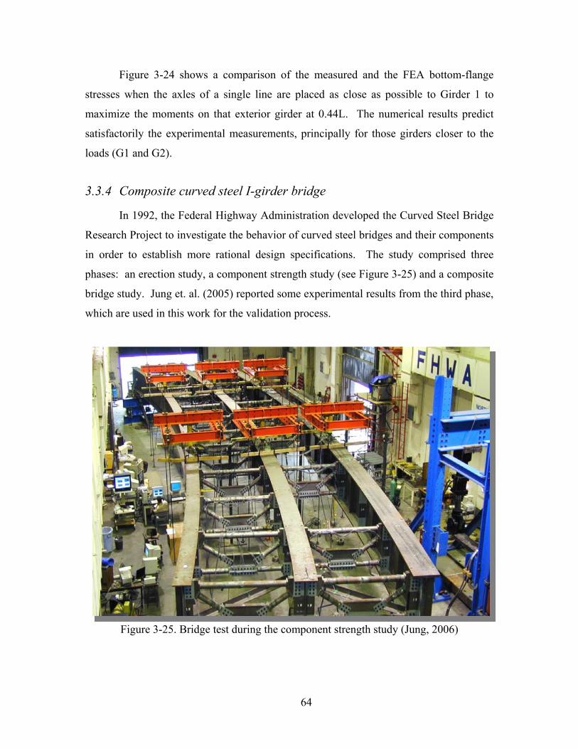
64
Figure 3-24 shows a comparison of the measured and the FEA bottom-flange
stresses when the axles of a single line are placed as close as possible to Girder 1 to
maximize the moments on that exterior girder at 0.44L. The numerical results predict
satisfactorily the experimental measurements, principally for those girders closer to the
loads (G1 and G2).
3.3.4 Composite curved steel I-girder bridge
In 1992, the Federal Highway Administration developed the Curved Steel Bridge
Research Project to investigate the behavior of curved steel bridges and their components
in order to establish more rational design specifications. The study comprised three
phases: an erection study, a component strength study (see Figure 3-25) and a composite
bridge study. Jung et. al. (2005) reported some experimental results from the third phase,
which are used in this work for the validation process.
Figure 3-25. Bridge test during the component strength study (Jung, 2006)

65
Figure 3-26 illustrates the cross section and plan view of the test bridge. The
cross section of the bridge consists of three prismatic I-girders spaced at 8.75ft and the
bridge span is 90ft measured along its centerline. The radii of curvature are 191.25ft,
200ft and 208.75 ft for the inside (G1), middle (G2) and outside (G3) girders,
respectively. All of the steel plates used A709 Gr.50 steel with the exception of the
bottom flange of G3 which used HPS 70W. The cast-in-place concrete slab is 8in thick
with 3in haunches and 3ft overhangs. The composite action between the slab and the
plate girders is given by studs (6in x ¾in) spaced at 6in both longitudinally and
transversely. The bridge has five equally spaced K-shaped cross frames, which are
strong enough to develop the ultimate capacity of the composite bridge system without
any cross-frame member failure.
a. Cross section of the test bridge
b. Plan view of the test bridge
Figure 3-26. Geometrical characterization of the bridge test (Jung, 2006)

66
The experimental results shown in Figure 3-27, Figure 3-28 and Figure 3-29
correspond to a testing loading that simulates the effects of two design trucks aligned
side-by-side at the middle of the bridge plus two lanes. This loading condition governs
the flexural design of G3. In general, a satisfactory agreement is observed between the
numerical and experimental results for the global response of the test bridge. Although
the model fails to predict the maximum positive LFB stresses, the maximum negative
LFB stresses (which are larger than the positive ones) seem to be adequately calculated.
0 5 10 15 20 250
200
400
600
800
1000
1200
1400
G3 Mid-span deflection (in)
Tota
l app
lied
load
(Kip
s)
FEA - NGFEA - JungExp.
Figure 3-27. Applied load vs. G3-mid-span deflection

67
0 50 100 150 200 250 300 350 400 4500
200
400
600
800
1000
1200
Reaction (Kips)
Tota
l app
lied
load
(Kip
s)
G3 - FEA NGG2 - FEA NGG1 - FEA NGExp.G3Exp.G2Exp.G1
Figure 3-28. Applied load vs. vertical reactions
0 0.1 0.2 0.3 0.4 0.5 0.6 0.7 0.8 0.9 1-20
-10
0
10
20
30
40
Normalized length
Stre
ss, σ
(Ksi
)
MAB - FEA NGLFB - FEA NGMAB - Exp.LFB - Exp.
Figure 3-29. G3 bottom flange stresses at a load level of 570Kips (MAB: Major-axis
bending, LFB: lateral flange bending)

68
3.4 Analyses
A user-defined sub-routine in Matlab® was used to create the input file for each
FE model that was analyzed by ABAQUS® Version 6.7.1, a commercially available
FEA software program. The initial loads such as the steel weight and the distributed
construction loads were applied using linear static stress analyses, since the structure
behaves within the elastic ranges without the presence of instabilities at this load level.
However, the concrete deck placement was simulated using a nonlinear static analysis to
consider probable material nonlinearity or geometrically nonlinear behavior causing
buckling or local instabilities.
The nonlinear analysis is based on the modified Riks algorithm available in
Abaqus®. This method has the ability to pass beyond the limit point and trace the
unloading portion of the nonlinear equilibrium path, as shown in Figure 3-30. The Riks
method uses the load magnitude as an additional unknown; it solves simultaneously for
loads and displacements. Therefore, another quantity must be used to measure the
progress of the solution. ABAQUS/Standard uses the “arc length,” l, along the static
equilibrium path in load-displacement space. This approach provides solutions regardless
of whether the response is stable or unstable (Abaqus, 2002).
Figure 3-30. Load-displacement response of an unstable system (Abaqus, 2002)

69
This method basically finds the solution of a single equilibrium path in a space
that is defined by the nodal variables and the loading parameter. The solution during each
increment is found by moving a given distance along the tangent line to the current
solution point and then searching for equilibrium in the plane that not only passes through
the point thus obtained, but also is orthogonal to the same tangent line. Once this plane is
determined, the Newton’s method is used to solve the equilibrium equations. It is
assumed that the response is reasonably smooth, i.e. sudden bifurcations do not occur.
The algorithm of the modified Riks method is shown in Figure 3-31, (Righman, 2005).
Figure 3-31. Modified Riks algorithm (Righman, 2005)

70
Chapter 4: Parametric study of the lateral flange bending during construction
A parametric study is used to investigate the effects of the deck-placement
process on the LFB of straight, skewed and curved steel I-girder bridges. The parametric
study is defined by: i. the parameters considered as significant in the response of the
structure; ii. the loads that represent the real conditions during the deck casting sequence;
iii. the design according to the code provisions of the parametric configurations; iv. the
models used to represent the physical behavior of the bridges; and v. the analyses defined
for each bridge configuration to represent the deck casting sequence.
4.1 Parameters
The selection of the variables in this work is intended to cover a wide range of
variation in the parameters that govern the practical design of skewed and curved steel
bridges. All bridge configurations have three spans arranged such that the end spans (Le)
are 80% of the middle span (Lm). This span configuration helps to assure an optimum
and homogeneous depth of the girders in all spans (NSBA, 2002). The cross sections
consist of four girders spaced at 12ft centers with 3.6ft deck overhangs. Structural steel
having a specified minimum yield stress of 50Ksi is used throughout. The deck is
conventional cast-in-place concrete with a specified minimum 28-day compressive
strength of 4Ksi. The total deck thickness is 9.5in, including a one-half inch integral
wearing surface. The concrete deck haunch is assumed to be 3.5in deep measured from
the top of the web to the bottom of the concrete deck. A future wearing surface of 25psf
is specified for design. Permanent steel deck forms of 15psf are also assumed to be used
between girders.
Table 4-1 presents the varying parameters considered in this project and their
corresponding values. Straight, skewed and curved bridge configurations (ST, SK and
CV) were generated for each middle span length (Lm) considered in the study, resulting in
a total of 21 hypothetical bridges without including the additional configurations

71
generated for each cross-frame spacing. Curved bridges with skewed supports were not
considered in this work.
Table 4-1. Varying parameters Parameter Value
Middle span length (Lm) 150ft – 240ft – 300ft
Ratio of Lm to radius of curvature (Lm/R) 0.30 – 0.45 – 0.60
Skew angle (θ) 0° - 30° - 45° - 60°
Range of cross-frame spacing (Lb) 22ft – 42ft
Bridge configurations using different cross-frame distances (Lb) were constructed
as indicated in Table 4-2 and Table 4-3 to analyze the variation of the LFB effects which
depend directly on this parameter.
Table 4-2. Cross-frame spacing for positive moment regions Lb (ft)
Bridge type End span, Le (ft) 120 192 240
ST, SK, CV Model Lb1 25 25 22
ST, SK, CV Model Lb2 27 28 27
ST, SK, CV Model Lb3 32 33 35
ST, SK, CV Model Lb4 37 39 37
ST Model Lb5 42 42 42
Middle span, Lm (ft) 150 240 300
ST, SK, CV Model Lb1 22 25 22
ST, SK, CV Model Lb2 27 27 28
ST, SK, CV Model Lb3 32 35 34
ST, SK, CV Model Lb4 40 37 38
ST Model Lb5 42 42 44
Table 4-3. Cross-frame spacing for negative moment regions Lb (ft)
Bridge type Middle span, Lm (ft) 150 240 300
ST, SK, CV Model Lb1 20 20 20
ST, SK, CV Model Lb2 21 26 24
ST, SK, CV Model Lb3 27 33 31
ST, SK, CV Model Lb4 35 36 36
ST Model Lb5 36 36 40

72
4.2 Loads
The loading condition corresponds to the loads acting during the deck casting
process: permanent dead loads and construction loads. Permanent dead loads include the
self weight of the structural members and construction loads comprise the following
elements (NSBA, 2002; KDoT, 2005):
• Overhang form brackets: 50 lb each, spaced every 3ft
• Formworks: 10 lb/ft2
• Screed rail: 85 lb/ft
• Railing: 25 lb/ft
• Walkway: 50 lb/ft2
• Finishing machine: 813 lb/wheel for a total of 4 wheels per exterior girder (see Figure
4-1 and Figure 4-2)
The factored loads correspond to the Strength Load Combination I of the
Specifications, which recommend that the load factors shall not be taken less than 1.25
and 1.5 for the dead and the construction loads, respectively (AASHTO, 2007).
Therefore, these recommended factors were used for the ultimate loads presented in this
work.
Figure 4-1. Visualization of the finishing machine on the exterior girder (KDT, 2005)

73
Figure 4-2. General view of a finishing machine (Bid-Well 4800)
4.2.1 Deck placement sequence
A symmetric deck placement sequence composed of three basic consecutive
stages was considered as shown in Figure 4-3, where the concrete is poured first in the
positive moment region of the end spans followed by that corresponding to the middle
span (NSBA, 2002). The sequence is completed by placing the concrete in the negative
moment regions over the pier zones. This sequence scheme is intended to minimize
cracking of the concrete slab primarily in the negative moment regions. Additional
intermediate stages are incorporated into the basic three-step sequence to consider the
effect of the finishing-machine wheels in the positive moment regions as shown in Figure
4-4.
Figure 4-3. Basic deck placement sequence

74
The LFB effects due to distributed (wu) and concentrated (Pu) loads were
evaluated separately in the positive moment regions. First, the effects of the distributed
loads are assessed from the casting stages that consider only the weight of the fresh
concrete, i.e. Castings 2 and 4 in Figure 4-4 for the end and middle spans, respectively.
Then, the concentrated load effects are analyzed from the casting stages that include the
finishing-machine wheels combined with the fresh concrete, i.e. Castings 1 and 3.
The negative moment regions are mostly controlled by the final stage from the
sequence shown in Figure 4-4. However, the maximum bending results in these regions
may be obtained at intermediate phases. Therefore, the complete casting sequence is
considered for the pier regions independent of the casting stage.
Figure 4-4. Detailed deck casting sequence

75
For skewed bridges, the deck placement was considered parallel to the supports.
The construction joints for curved and skewed bridges are radial and parallel to the skew
angle, respectively.
4.3 Structural design
Girders, cross frames and stiffeners of the straight bridge configurations were
sized according to 2007 AASHTO Specifications, based on the parameters and loads
defined previously. Changes of section that coincide with the construction joints are
assumed in regions close to the piers, as shown in Figure 4-3. Table 4-4 includes the
girder plate sizes for the different cross sections employed at the straight bridges. The
same sections were used for the skewed and curved bridges analyzed in this work to
achieve one of the research objectives consisting of finding the maximum available skew
angle and curvature for bridges originally designed as straight.
Table 4-4. Girder plate sizes
Lm (ft) End Span
S1
Pier Zone
S2
Middle Span
S3
150
TF: 20”x1”
BF: 20”x1”
W: 60”x ½”
LS: 96ft
TF: 18”x2”
BF: 20”x2”
W: 60”x ½”
LS: 54ft
TF: 16”x7/8”
BF: 18”x1”
W: : 60”x ½”
LS: 90ft
240
TF: 24”x1½”
BF: 24”x1¼”
W: 80”x5/8”
LS: 154ft
TF: 28”x2¾”
BF: 28”x2¾”
W: 80”x5/8”
LS: 86ft
TF: 20”x1¼”
BF: 24”x1¼”
W: 80”x5/8”
LS: 144ft
300
TF: 28”x1¼”
BF: 28”x1¼”
W: 105”x¾”
LS: 192ft
TF: 32”x2¾”
BF: 32”x2¾”
W: 105”x¾”
LS: 108ft
TF: 26”x1¼”
BF: 26”x1¼”
W: 105”x¾”
LS: 180ft
TF: Top Flange; BF: Bottom Flange; W: Web; LS: Length of the section
For design purposes, the cross frames of each straight bridge were arranged such
that their maximum spacing (Lb) in the positive-moment regions was close to the

76
traditional spacing used in practice, 25ft. However, in the pier regions the cross frames
were set at shorter distances (17ft – 20ft), as indicated in Table 4-5.
Table 4-5. Cross-frame spacing, Lb (ft) End Span Middle Span
Lm (ft) M+ M- M- M+
150 25 20 20 22
240 25 17 20 25
300 22 20 18 22
4.4 Models
A FE model was developed for each straight, skewed and curved bridge
configuration using a MATLAB® code that generates the input files which are
subsequently processed by Abaqus®. Figure 4-5 shows a typical FE model of a curved
bridge configuration at the end of Casting 2.
Figure 4-5. Finite element model of a typical curved bridge configuration

77
As discussed in Chapter 3, four-node shell elements with reduced integration and
enhanced hourglass control were used to model the plate girders and the concrete slab.
The deck composite action was simulated using rigid elements that connect the top
flanges of the girders to the slab. The cross frames and the stiffeners were modeled using
slender beam elements based on the Euler-Bernoulli formulation, assuming a linear
section behavior. The mesh configuration in the flanges employs six elements across the
flange width with aspect ratios close to four. An aspect ratio close to one was selected
for the webs. All shell elements in the girders are approximately 12-inch long.
In addition, the stay-in-place (SIP) forms were included in the modeling process
of the bridges when the girders act in a non-composite state. This inclusion was required
to identify the position of the shell elements that represent the concrete deck after the
non-composite girders have deformed during the placement of the fresh concrete. The
deck formwork was modeled by shell elements with the same coordinates as those
elements used to model the concrete deck, but with a lower stiffness represented by the
thickness (t=2in) and the material (E=33.2ksi). Figure 4-6 shows the bending stresses in
the top flange of a curved bridge model with and without including the stay-in-place
forms. It is observed that the fbu is practically not affected by the inclusion of the forms,
while the LFB decreases up to 20% in regions of maximum moment in a curved bridge
model. In addition, the forms provide stability to the inner girder of curved bridges, since
the LFB varies regularly about the zero stress instead of exhibiting a global buckling
mode. The decreasing effect on the LFB due to the inclusion of the deck formwork is
also exhibited by the skewed and straight bridges, but to a much lesser degree.
The continuity over the intermediate supports also contributes to reduce the levels
of LFB due to the increase of the structural stiffness. In addition, the LFB of a non-
composite segment due to fresh concrete is relieved when previous casts are considered
as composite in the analyses.
The vertical loads other than the self weight of the steel members are considered
in the models using concentrated forces applied directly on the girder nodes. The self
weight of steel was included as an element-based body load due to gravity. On the other
hand, the torsional effects produced by the overhang loads are represented on the exterior
girders by horizontal forces as shown in Figure 4-7. A maximum depth of 70in is used

78
for the overhang brackets. However, this distance varies for each bridge configuration
according to the web depth and the FE dimensions.
SIP forms No SIP forms
Exterior Girder
0 0.05 0.1 0.15 0.2 0.25 0.3 0.35 0.4 0.45 0.5-50
-40
-30
-20
-10
0
10
20
30
40
50
Stre
ss (K
si)
fbufl flange tip 1fl flange tip 2
0 0.05 0.1 0.15 0.2 0.25 0.3 0.35 0.4 0.45 0.5
fbufl flange tip 1fl flange tip 2
Interior Girder
0 0.05 0.1 0.15 0.2 0.25 0.3 0.35 0.4 0.45 0.5-50
-40
-30
-20
-10
0
10
20
30
40
50
Normalized distance
Stre
ss (K
si)
fbufl flange tip 1fl flange tip 2
0 0.05 0.1 0.15 0.2 0.25 0.3 0.35 0.4 0.45 0.5Normalized distance
fbufl flange tip 1fl flange tip 2
Figure 4-6. Effect of the stay-in-place forms in the bending stresses of a curved bridge

79
Figure 4-7. Torsional effects on exterior girders produced by overhang loads
4.5 Analyses
Five static stress analyses are required for each bridge configuration to simulate
the deck placement, as shown in Figure 4-8. The arrows in the figure point to the
previous analysis from where the initial conditions are taken. As mentioned before, the
weight of the wet concrete slab is considered in the corresponding cast as explicit
concentrated loads applied directly on the non-composite girders. However, in the
analyses, earlier concrete casts are made composite for each subsequent cast.
End spans Middle Span Pier regions
Casting 1:Pu and wu
Casting 2: wu Casting 3: Pu and wu
Casting 4: wu Casting 5: Pu and wu
Figure 4-8. Sequence of analysis for each bridge configuration

80
A detailed explanation of each one of the casting stages and the corresponding
models from Figure 4-8 is given below:
• End spans:
Casting 1: The initial conditions are zero for this cast. The loads applied
sequentially consist of: i. the weight of the steel superstructure, ii. the construction loads
without considering the finishing machine, and iii. the weight of the fresh concrete
corresponding to one-half of the positive moment regions at the end spans along with the
finishing machine.
Casting 2: In this cast, the initial conditions are also assumed as zero since the
fresh concrete of the positive moment regions at the end spans is applied at once.
Therefore, the load sequence is similar to the one described for Casting 1. However, in
this case, the fresh concrete is applied over the complete positive moment regions of the
end spans without including the finishing machine effects.
• Middle span:
Casting 3: The initial conditions correspond to the final stresses and deformations
obtained in Casting 2. In this stage, the shell elements of the concrete deck
corresponding to Casting 1 need to be initially activated. Then, the weight of the fresh
concrete is applied over one-half of the positive moment region of the middle span,
including the finishing machine.
Casting 4: The difference between Castings 3 and 4 consists in that the weight of
the fresh concrete in Casting 4 is applied over the complete positive moment region of
the middle span, and the finishing machine effects are neglected.
• Pier regions:
Casting 5: The initial conditions are taken from the final response of Casting 4.
The shell elements corresponding to the concrete slab placed in Casting 2 are activated to
simulate the composite action in this zone. In this cast, the weight of the fresh concrete is
extended from the beginning of the negative moment regions at the end spans to the
midpoint between the pier and the end of the negative moment regions at the middle
span. The finishing machine effects are included as well.

81
Chapter 5: Approximation of the lateral flange bending in steel I-girder bridges
This chapter presents the methods used to approximate the LFB in straight,
skewed and curved steel I-girder bridges due to construction loads during deck placement
based on the results obtained from the parametric study described in Chapter 4. The
major-axis bending stresses are analyzed as well. However, the principal contribution to
estimate fbu is made for curved bridges since it is shown that the torsional effects do not
affect the vertical bending response in straight and skewed bridges.
5.1 Definition of the bending stresses from FEA
The approximations proposed in this work to estimate the bending effects in steel
I-girder bridges during deck placement are based on the results obtained from the FEA of
the parametric bridge configurations. However, the direct response obtained from the
Abaqus® output corresponds to the total bending stresses at each flange tip (f1 and f2), as
shown in Figure 5-1. Therefore, a Matlab® code was developed to compute the major-
axis bending (fbu) and LFB (fl) stresses from f1 and f2 assuming a linear response, as
follows:
1 2
2buf ff +
= 5-1
l total buf f f= − 5-2
Figure 5-1. Identification of fl and fbu from the total flange bending response

82
For example, the resulting bending stresses computed in Matlab® for the top and
bottom flanges of the exterior girder in a curved bridge model are shown in Figure 5-2.
0 0.05 0.1 0.15 0.2 0.25 0.3 0.35 0.4 0.45 0.5-50
-40
-30
-20
-10
0
10
20
30
40
50
Normalized distance
Stre
ss (K
si)
Top Flange G4 - Casting 2
fbufl flange tip 1fl flange tip 2
0 0.05 0.1 0.15 0.2 0.25 0.3 0.35 0.4 0.45 0.5Normalized distance
Bottom Flange G4 - Casting 2
fbufl flange tip 1fl flange tip 2
Figure 5-2. Bending stresses on the exterior girder of a curved bridge model
5.1.1 Parametric Notation
The effects on fl and fbu of the deck placement loads are evaluated in this project
using the following parametric notation:
• Span lengths: The span lengths of the bridge models are identified by referencing
their middle span length (Lm=150ft, 240ft or 300ft) only, since the end span lengths
depend on Lm (Le=80%Lm).
• Flange position: Top flange (TF) or bottom flange (BF).
• Girder section: S1 for the section corresponding to the positive moment regions of
Le, S2 for the negative moment regions over the piers, and S3 for the positive moment
region of Lm.
• Casting sequence and load type: These variables are related to each other since the
effects of the distributed loads (wu) are evaluated from Castings 2 and 4 for S1 and
S3, respectively. The concentrated load effects (Pu) are analyzed from Castings 1
and 3 for S1 and S3, since these casts include the finishing-machine wheels combined
with the fresh concrete. For S2, the complete casting sequence is considered.

83
• Girder position: This parameter is particularly important for curved bridges to
indicate the position of the girder with respect to the curvature (outside G4 and inside
G1).
• Skew angle (θ): 30°, 45° or 60°.
• Curvature angle (Lm/R): 0.30, 0.45 or 0.60
• Bridge type: Straight bridges (ST-0), skewed bridges with θ=30°, 45° or 60° (SK30,
SK45 or SK60), and curved bridges with L/R=0.30, 0.45 or 0.60 (CV30, CV45 or
CV60).
• Cross-frame orientation in skewed bridges: Perpendicular to the girders (xf1) and
parallel to the abutments (xf2).
5.1.2 Normalization of the LFB
The LFB stresses obtained from FEA are normalized in order to establish fitting
models independent of the cross section properties. Therefore, the numerical stresses, fl,
are multiplied by the flange section modulus, Sf, to obtain the lateral flange moment, Mlat.
Then, the lateral moment is divided by the corresponding lateral load which depends
directly on the overhang bracket depth for construction loads, or the web depth for
curvature effects. Consequently, the following expressions were used to present the LFB
effects in this work:
l f lat
l l
f S MF F
= 5-3
l f lat
l l
f S MP P
= 5-4
where Fl and Pl are the lateral distributed and concentrated loads that represent the
torsional effects.
5.2 Overhang loads in straight bridges
The LFB effects produced by distributed and concentrated loads are studied
initially from the straight bridge configurations where the curvature and skew effects do
not take place.

84
5.2.1 Major-axis bending, fbu
Figure 5-3 shows that the major-axis bending exhibited by the exterior girders of
straight bridges is independent of the cross-frame spacing. Therefore, fbu may be taken
directly from FEA using any cross-frame distance.
22 24 26 28 30 32 34 36 38 40 42-25
-20
-15
-10
-5
0
5
10
15
20
25G4 ST-0-S1 for wu
Lb (ft)
fbu
(Ksi
)
150ft-TF150ft-BF240ft-TF240ft-BF300ft-TF300ft-TF
22 24 26 28 30 32 34 36 38 40 42
G4 ST-0-S1 for Pu
Lb (ft)
150ft-TF150ft-BF240ft-TF240ft-BF300ft-TF300ft-TF
Figure 5-3. Effect of the cross-frame spacing in the major-axis bending
5.2.2 Positive Moment Regions
5.2.2.1 Lateral distributed load effect
For distributed loads in the positive moment regions, the LFB stresses were
approximated using the following fitting model: a
lat b
l
M Lwu A
= 5-5
where wul is the lateral distributed load due to fresh concrete and Lb is the cross-frame
spacing. The variables a and A are defined in Table 5-1 for both top and bottom flanges.
Figure 5-4 compares the results obtained using the proposed equation (Eq. 5-5) with the
effects given by FEA and the code approximate equation (Eq. 1-2). It is observed that the
code equation is highly conservative in all cases, principally for large cross-frame
distances. However, the proposed equation predicts satisfactorily the LFB at the exterior

85
girders of the end span over the entire range of cross-frame distances. Although the LFB
exhibited in the middle span is slightly lower, the same equations are proposed for Lm to
simplify the recommended approximations for straight bridges.
Table 5-1. Fitting parameters for distributed loads in straight bridges (Positive Moment).
a A
(fta-2)
TF 1.22 2.46
BF 1.92 29.24
20 25 30 35 40 450
20
40
60
80
100
120
140
160
180G4 ST-0-S1 for wu, TF
Mla
t/wul
(ft2 )
150ft-FEA240ft-FEA300ft-FEACode Eq.Proposed Eq.
20 25 30 35 40 45
G4 ST-0-S1 for wu, BF
150ft-FEA240ft-FEA300ft-FEACode Eq.Proposed Eq.
20 25 30 35 40 450
20
40
60
80
100
120
140
160
180G4 ST-0-S3 for wu, BF
Lb (ft)
Mla
t/wul
(ft2 )
150ft-FEA240ft-FEA300ft-FEACode Eq.Proposed Eq.
20 25 30 35 40 45
G4 ST-0-S3 for wu, BF
Lb (ft)
150ft-FEA240ft-FEA300ft-FEACode Eq.Proposed Eq.
Figure 5-4. LFB due to distributed loads in the positive moment regions of straight
bridges

86
5.2.2.2 Lateral concentrated load effect
The evaluation of the concentrated load effects on LFB is more complex than for
distributed loads due to several reasons:
• Both distributed and concentrated loads act simultaneously in Castings 1 and 3.
• The position of concentrated loads at the corresponding cross-frame spacing depends
on the cross-frame distribution, i.e. the wheel loads may be located over one cross-
frame location or anywhere within two consecutive cross frames. For example, a
simply supported straight bridge was analyzed separately to identify the effect of the
concentrated load position on the LFB. Figure 5-5 shows that a linear trend parallel
to the code equation is followed by models where the load is placed at the middle of a
cross-frame spacing, being the critical location. However, other intermediate
positions decrease the LFB effect.
15 20 25 30 35 40 45 500
0.2
0.4
0.6
0.8
1
1.2
1.4G2 fl, TF
fl (K
si)
Lb (ft)
FEACodePu at the middle of LbPu close to a XF postion
Figure 5-5. Effect of the concentrated load position in the LFB
• A similar situation occurs for distributed loads which extend up to the position of the
leading wheel in the finishing machine.
• The finishing machine effect on an exterior girder consists of four wheels acting
within a distance of 8ft. However, in the approximated equations, it is conservatively
assumed that the forces are all applied at the same point.

87
22 24 26 28 30 32 34 36 38 40 420
1
2
3
4
5
6
7
8
9
10M
lat/4
Pul
(ft)
G4 ST-0-S1 for Pu, TF
150ft-FEA240ft-FEA300ft-FEACode Eq.Proposed Eq.
22 24 26 28 30 32 34 36 38 40 42
G4 ST-0-S1 for Pu, BF
150ft-FEA240ft-FEA300ft-FEACode Eq.Proposed Eq.
22 24 26 28 30 32 34 36 38 40 420
1
2
3
4
5
6
7
8
9
10
Lb (ft)
Mla
t/4P
ul (f
t)
G4 ST-0-S3 for Pu, TF
150ft-FEA240ft-FEA300ft-FEACode Eq.Proposed Eq.
22 24 26 28 30 32 34 36 38 40 42Lb (ft)
G4 ST-0-S3 for Pu, BF
150ft-FEA240ft-FEA300ft-FEACode Eq.Proposed Eq.
Figure 5-6. LFB due to concentrated loads in straight bridges (Positive Moment).
Consequently, a linear model similar to the code equation was adopted in this
work to describe the combined effect of the lateral concentrated load, Pul, representing a
single wheel with the distributed load due to fresh concrete. However, the model only
considers explicitly the concentrated loads while the concrete effect is considered by the
combination of the variables B and C, as follows:
4lat b
l
M L CPu B
= + 5-6
The results of the models are shown in Table 5-2 and Figure 5-6. It is observed
that the linear regression considers the most external points from the critical curves, since
these points correspond to models where the concentrated loads are placed at the middle

88
of a cross-frame spacing. It is also noticed that the proposed equation for the bottom
flange governs over the code equation for cross-frame distances larger than 26ft.
However, both the code and the proposed approximations coincide for the top flange.
Table 5-2. Fitting parameters for concentrated loads in straight bridges (Pos. Moment).
B C
(ft)
TF 8 0
BF 3.5 -4.2
5.2.3 Negative Moment Regions
The LFB effect on the negative moment regions was approximated considering
only the distributed loading case since the contribution from the concentrated loads is
negligible. Therefore, Equation 5-5 is taken as a valid model with the corresponding
fitting parameters contained in Table 5-3. Figure 5-7 shows that the proposed equation
satisfactorily predicts the LFB in both flanges.
Table 5-3. Fitting parameters for distributed loads in straight bridges (Neg. Moment)
a A
(fta-2)
TF 1.37 4.42
BF 2.02 22.45
20 22 24 26 28 30 32 34 36 38 400
20
40
60
80
100
120
140G4 ST-0-S2 for wu, TF
Lb (ft)
Mla
t/wul
(ft2 )
150ft-FEA240ft-FEA300ft-FEACode Eq.Proposed Eq.
20 22 24 26 28 30 32 34 36 38 40
G4 ST-0-S2 for wu, BF
Lb (ft)
150ft-FEA240ft-FEA300ft-FEACode Eq.Proposed Eq.
Figure 5-7. LFB effects due to concentrated loads in straight bridges (Neg. Moment).

89
5.3 Overhang loads in skewed bridges
In all skewed bridges, the concrete is placed parallel to the skew. An evaluation
of the cross-frame orientation was initially performed using bridge configurations with
Lm=150ft. Then, the bending effects in skewed bridges are analyzed employing models
with the recommended cross-frame orientation.
5.3.1 Cross-frame orientation
Figure 5-8 compares the bending results exhibited by the top flange of an exterior
girder in a straight and skewed bridge subjected to vertical loads, e.g. steel weight. The
results indicate that skewed bridges exhibit LFB even when torsional loads are not
applied. However, in the presence of torsional effects, the LFB effect is slightly more
pronounced when the cross frames are oriented parallel to the supports as shown in
Figure 5-9. Therefore, a perpendicular orientation of the cross frames is recommended
for general skewed bridges to increase the lateral stiffness of the structure, hence it is
used in the models described next to evaluate the bending effects.
Straight Bridge Skewed Bridge with θ=45°
0 0.05 0.1 0.15 0.2 0.25 0.3 0.35 0.4 0.45 0.5-5
-4
-3
-2
-1
0
1
2
3
4
5
Normalized distance
Stre
ss (K
si)
fbufl flange tip 1fl flange tip 2
0 0.05 0.1 0.15 0.2 0.25 0.3 0.35 0.4 0.45 0.5Normalized distance
fbufl - flange tip 1fl - flange tip 2
Figure 5-8. Effect of the skew angle in the LFB exhibited by the top flange

90
Top Flange G4 Bottom Flange G4
20 25 30 35 40 4520
40
60
80
100
120
140
160
180M
lat/w
ul (f
t2 )
Lb (ft)
XF PerpendicularXF ParallelCode Eq.
20 25 30 35 40 45Lb (ft)
XF PerpendicularXF ParallelCode Eq.
Figure 5-9. Effect of the cross-frame orientation in the LFB of skewed bridges
5.3.2 Major-axis bending, fbu
Figure 5-10 shows that the major-axis bending in skewed bridges is not only
independent of the cross-frame spacing but also of the skew angle. Therefore, fbu may be
taken from FEA performed for skewed bridges with any cross-frame spacing and skew
angle, including their straight counterpart.
5.3.3 Positive Moment Regions
An approach analogous to the procedure described for straight bridges was
followed to approximate the LFB due to distributed and concentrated loads in the positive
moment regions of skewed bridges.

91
20 25 30 35 40 45-25
-20
-15
-10
-5
0
5
10
15
20
25G4 -sk30xf1-S1 for wu
Lb (ft)
fbu
(Ksi
)
150ft-TF150ft-BF240ft-TF240ft-BF300ft-TF300ft-TF
20 25 30 35 40 45
G4 -sk45xf1-S1 for wu
Lb (ft)
150ft-TF150ft-BF240ft-TF240ft-BF300ft-TF300ft-TF
20 25 30 35 40 45-25
-20
-15
-10
-5
0
5
10
15
20
25G4 -sk60xf1-S1 for wu
Lb (ft)
fbu
(Ksi
)
150ft-TF150ft-BF240ft-TF240ft-BF300ft-TF300ft-TF
Figure 5-10. Effect of the skew angle in the major-axis bending
5.3.3.1 Distributed load
The corresponding fitting parameters are indicated in Table 5-4. Figure 5-11
shows the normalized LFB for bridges with θ=30° (see Appendix A for θ=45° and 60°).
It is observed that the code recommended equation (Eq. 1-2) significantly overestimates
the LFB principally for long cross-frame distances. However, the code fails to predict the
LFB exhibited by the bottom flange of bridges with low Lb values, especially for high
skew angles. For that reason, a lower limit equal to 30, 45 and 70ft2 for θ=30°, 45° and
60°, respectively, was introduced in the proposed equation for the normalized LFB at the
bottom flange.

92
Table 5-4. Fitting parameters for distributed loads in skewed bridges (Pos. Moment).
a A
(fta-2)
θ 30° 45° 60° 30° 45° 60°
TF 1.44 1.26 1.41 3.59 1.73 2.31
BF 1.29 1.13 1.26 2.19 1.00 1.42
20 25 30 35 40 450
20
40
60
80
100
120
140
160
180G4 SK-sk30xf1-S1 for wu, TF
Mla
t/wul
(ft2 )
120ft-FEA192ft-FEA240ft-FEACode Eq.Proposed Eq.
20 25 30 35 40 45
G4 SK-sk30xf1-S1 for wu, BF
120ft-FEA192ft-FEA240ft-FEACode Eq.Proposed Eq.
20 25 30 35 40 450
20
40
60
80
100
120
140
160
180G4 SK-sk30xf1-S3 for wu, TF
Mla
t/wul
(ft2 )
Lb (ft)
150ft-FEA240ft-FEA300ft-FEACode Eq.Proposed Eq.
20 25 30 35 40 45
G4 SK-sk30xf1-S3 for wu, BF
Lb (ft)
150ft-FEA240ft-FEA300ft-FEACode Eq.Proposed Eq.
Figure 5-11. LFB due to distributed loads in skewed bridges (Positive Moment).
5.3.3.2 Concentrated loads
Table 5-5 contains the definition of the variables B and C from the fitting model
for concentrated loads according to the numerical stresses obtained in the parametric

93
study. Figure 5-12 (including the figures from Appendix A) shows that the code equation
fails to predict satisfactorily the LFB in most of the cases, principally for the bottom
flange.
Table 5-5. Fitting parameters for concentrated loads in skewed bridges (Pos. Moment). B C (ft)
θ 30° 45° 60° 30° 45° 60°
TF 8 7.4 7.4 0 0 1.5
BF 4.5 5.0 14 -2.0 0 6.0
20 25 30 35 40 450
1
2
3
4
5
6
7
8G1 SK-sk30xf1-S1 for Pu, TF
Mla
t/4P
ul (f
t)
120ft-FEA192ft-FEA240ft-FEACode Eq.Proposed Eq.
20 25 30 35 40 45
G4 SK-sk30xf1-S1 for Pu, BF
120ft-FEA192ft-FEA240ft-FEACode Eq.Proposed Eq.
20 25 30 35 40 450
1
2
3
4
5
6
7
8G1 SK-sk30xf1-S3 for Pu, TF
Mla
t/4P
ul (f
t)
Lb (ft)
150ft-FEA240ft-FEA300ft-FEACode Eq.Proposed Eq.
20 25 30 35 40 45
G1 SK-sk30xf1-S3 for Pu, BF
Lb (ft)
150ft-FEA240ft-FEA300ft-FEACode Eq.Proposed Eq.
Figure 5-12. LFB due to concentrated loads in skewed bridges (Positive Moment)

94
5.3.4 Negative Moment Regions
The LFB in negative moment regions was approximated by a constant term that
depends on the skew angle. This term was defined according to the numerical results as
4, 6 and 8Ksi for θ=30°, 45° and 60°, respectively. The constant approximation is
proposed to conservatively estimate the stresses which do not exhibit a consistent trend.
Figure 5-13 presents the LFB stresses for bridge configurations with θ=30°, the
remaining figures corresponding to θ=45° and 60° are contained in Appendix A. The
results indicate that the code recommendation of using 10Ksi for the unfactored LFB
stresses in skewed bridges is conservative even compared to factored stresses.
10 15 20 25 30 35 400
2
4
6
8
10
12G4 SK-sk30xf1-S2 for wu, TF
fl (K
si)
Lb (ft)
150ft-FEA240ft-FEA300ft-FEACode Eq.Proposed Eq.
0 15 20 25 30 35 40
G1 SK-sk30xf1-S2 for wu, BF
Lb (ft)
150ft-FEA240ft-FEA300ft-FEACode Eq.Proposed Eq.
Figure 5-13. LFB effects due to distributed loads in skewed bridges (Neg. Moment).
5.4 Overhang loads in curved bridges
The evaluation of the bending stresses in curved bridges indicates that fbu and fl
are deeply affected by the curvature. In addition, the results showed that the participation
of the overhang loading term in the LFB effects is low compared to the curvature effects.

95
5.4.1 Major-axis bending, fbu
Figure 5-14 shows that the fbu in curved bridges is independent of Lb but is
affected by the curvature and the girder position. These relationships will be described in
detail below.
25 30 35 40-30
-20
-10
0
10
20
30G4 CV-S1 for wu
Lb (ft)
fbu
(Ksi
)
L/R=0.30-TFL/R=0.30-BFL/R=0.45-TFL/R=0.45-BFL/R=0.60-TFL/R=0.60-TF
25 30 35 40
G1 CV-S1 for wu
Lb (ft)
L/R=0.30-TFL/R=0.30-BFL/R=0.45-TFL/R=0.45-BFL/R=0.60-TFL/R=0.60-TF
Figure 5-14. Effect of curvature in the major-axis bending
5.4.2 Positive Moment Regions
5.4.2.1 Distributed loading effect
5.4.2.1.1 Major-axis bending, fbu
The proposed linear model intended to estimate fbu in curved bridges during
construction is given by:
( ) ( )max
max
1 2bu
buo
f Lsign b sign cf R
⎛ ⎞= +⎜ ⎟⎝ ⎠
5-7
where fbu max is the maximum major-axis bending stress and fbuo max is the maximum
major-axis bending stress of the straight counterpart (L/R=0). Table 5-6 and Table 5-7
contain the variables b and c, and the sign combinations (sign1, sign2) for the bridge
models evaluated in this project. Figure 5-15 and Figure 5-16 show that the major-
bending stresses increase linearly with the curvature at the end spans. Conversely, a

96
constant term is proposed for the middle span since fbu is not significantly affected by the
curvature over this zone.
Table 5-6. Fitting parameters for fbu due to distributed loads curved bridges (Pos.
Moment) Lm=150ft Lm =240ft Lm =300ft
b c b c b c
Outer Girder, G4: End span, Le 0.95 1 1.3 1 1.5 1
Outer Girder, G4: Middle span, Lm 0 1 0 1 0 1.1
Inner Girder, G1: End span, Le 0.85 1 1.06 1 1.2 1
Inner Girder, G1: Middle span, Lm 0 1 0 1 0 1.1
0 0.1 0.2 0.3 0.4 0.5 0.6 0.7-2
-1.5
-1
-0.5G4 - S1 for wu, TF
fbu/
|fbuo
|
Lm=150ft-FEALm=150ft-Eq.Lm=240ft-FEALm=240ft-Eq.Lm=300ft-FEALm=300ft-Eq.
0 0.1 0.2 0.3 0.4 0.5 0.6 0.7
G4-S1 for wu, BF
Lm=150ft-FEALm=150ft-Eq.Lm=240ft-FEALm=240ft-Eq.Lm=300ft-FEALm=300ft-Eq.
0 0.1 0.2 0.3 0.4 0.5 0.6 0.7-2
-1.5
-1
-0.5G4-S3 for wu, TF
fbu/
|fbuo
|
Lm/R
Lm=150ft-FEALm=150ft-Eq.Lm=240ft-FEALm=240ft-Eq.Lm=300ft-FEALm=300ft-Eq.
0 0.1 0.2 0.3 0.4 0.5 0.6 0.7
G4-S3 for wu, BF
Lm/R
Lm=150ft-FEALm=150ft-Eq.Lm=240ft-FEALm=240ft-Eq.Lm=300ft-FEALm=300ft-Eq.
Figure 5-15. Normalized fbu due to distributed loads in outer girders (Positive Moment)

97
Table 5-7. Sign combination used to estimate fbu (Sign1, Sign2) (Pos. Moment) Top flange, TF Bottom Flange, BF
G4 - , - + , +
G1 + , - - , +
0 0.1 0.2 0.3 0.4 0.5 0.6 0.7-1.5
-1
-0.5
0G1-S1 for wu, TF
fbu/
|fbuo
|
Lm=150ft-FEALm=150ft-Eq.Lm=240ft-FEALm=240ft-Eq.Lm=300ft-FEALm=300ft-Eq.
0 0.1 0.2 0.3 0.4 0.5 0.6 0.7
G1-S1 for wu, BF
Lm=150ft-FEALm=150ft-Eq.Lm=240ft-FEALm=240ft-Eq.Lm=300ft-FEALm=300ft-Eq.
0 0.1 0.2 0.3 0.4 0.5 0.6 0.7-2
-1.5
-1
-0.5G1-S3 for wu, TF
fbu/
|fbuo
|
Lm/R
Lm=150ft-FEALm=150ft-Eq.Lm=240ft-FEALm=240ft-Eq.Lm=300ft-FEALm=300ft-Eq.
0 0.1 0.2 0.3 0.4 0.5 0.6 0.7
G1-S3 for wu, BF
Lm/R
Lm=150ft-FEALm=150ft-Eq.Lm=240ft-FEALm=240ft-Eq.Lm=300ft-FEALm=300ft-Eq.
Figure 5-16. Normalized fbu due to distributed loads in inner girders (Pos. Moment)
5.4.2.1.2 Lateral flange bending, fl
The LFB stresses were approximated considering a hypothetical curved I girder
subjected to a uniform vertical distributed load, wu. The girder has a radius of curvature,
R, and a span length, L, that subtends an angle θ, as shown in Figure 5-17. The

98
eccentricity, d, between the vertical load and the straight line that connects the end
supports is a function of the longitudinal position. The maximum eccentricity, dmax, is at
the middle of the span length (Eq. 5-8). As a result of this eccentricity, a distributed
torsional moment, T, is generated along the girder which is equivalent to a couple of
horizontal distributed forces acting on the flanges, wul, as shown in Figure 5-18. The
magnitude of wul varies from zero at the end supports to the maximum value at the
middle of the span, wulmax (Eq. 5-9), as indicated by Figure 5-19. Therefore, the
maximum LFB stress, fl, will correspond to the cross-frame spacing, Lb, closer to the span
midpoint. The variation of wul along the central cross-frame spacing is assumed to be
small and consequently may be considered uniformly distributed. Finally, fl is
approximated by Equation 5-10 where a curve fitting process is required to define the
order of the approximation, d, and the denominator, D.
Figure 5-17. Hypothetical curved girder to approximate the curvature effects

99
Figure 5-18. Visualization of the torsional effects due to curvature
Figure 5-19. Horizontal distributed force on the top flange
max 1 cos2
d R θ⎛ ⎞= −⎜ ⎟⎝ ⎠
5-8
maxmax
uul
w dwh
= 5-9
maxd
ul bl
f
w LfDS
= 5-10

100
The LFB for curved girders is caused by two different sources: the curvature and
the overhang loads during construction. The curvature and the overhang torsional effects
have the same direction in the outer girder while they counteract at the inner girder, as
follows:
( ) ( )( ) ( )
. .
. .
max
for G4
for G1lat lat latcurv ov
lat lat latcurv ovd a
ul b l blat
M M M
M M M
w L wu LMD A
= +
= −
= ±
5-11
However, the participation of the overhang loading in the LFB is low compared to
the curvature effects as shown in Figure 5-20. In fact, the overhang-to-curvature effect
ratio reduces as the length of the span and the curvature increase. Therefore, the total
LFB is estimated using the curvature term only. However, the torsional effects due to
overhang loads are implicitly considered since the curve fitting process to estimate the
parameters d and D in Equation 5-10 is applied to the total LFB obtained from the
parametric study.
The critical case between the top and bottom flanges was selected to define the
proposed equations for curved bridges. The corresponding variables from the curve
fitting process are contained in Table 5-8 and Table 5-9. It is observed from Figure 5-21
that the LFB effects of the end spans are practically unaffected by the variation of the
curvature, while a slight effect is observed in the middle spans. The proposed equation
(Eq. 5-10) works adequately in both exterior girders. Significant reductions were found
in most of the cases compared to the estimations given by the AASHTO approximation
(Eq. 1-1). The major-axis bending moment, M, in the code equation was computed using
both the numerical and the estimated (Eq. 5-7) major-axis bending stresses, obtaining
similar results. This is a practical observation since the LFB in a curved bridge can be
approximated using the code equation (Eq. 1-1) together with the fbu computed from the
information of the straight counterpart. However, the figures contained in Appendix B
for Lm=240ft and 300ft indicate that the code equation fails to predict the LFB at the inner
girder of highly curved bridges with long spans. Therefore, it is recommended to use the
equation proposed in this work which predicts satisfactorily the LFB in all cases.

101
Figure 5-20. Comparison of the overhang and curvature effects in the LFB

102
Table 5-8. Fitting parameters for distributed loads in the outer girders (Pos. Moment) Section 150ft 240ft 300ft
d D
(ftd-2) d
D
(ftd-2) d
D
(ftd-2)
S1 1.99 31.14 1.32 2.49 1.72 9.55
S3 1.99 89.42 1.81 55.6 - -
Table 5-9. Fitting parameters for distributed loads in inner girders (Pos. Moment) Section 150ft 240ft 300ft
d D
(ftd-2) d
D
(ftd-2) d
D
(ftd-2)
S1 2.52 396.4 2.36 262.4 0.81 1.06
S3 2.31 443.2 2.51 839.7 - -
20 25 30 35 40 450
10
20
30
40
50
60
70
80
90
100G4 CV-S1 for wu, TF
Mla
t/wul
max
(ft2 )
L/R=0.30-FEAL/R=0.30-Code Mu-FEAL/R=0.30-Code Mu-Eq.L/R=0.45-FEAL/R=0.45-Code Mu-FEAL/R=0.45-Code Mu-EqL/R=0.60-FEAL/R=0.60-Code Mu-FEAL/R=0.60-Code Mu-Eq.Proposed Eq.
20 25 30 35 40 45
G4 CV-S1 for wu, BF
L/R=0.30-FEAL/R=0.30-Code Mu-FEAL/R=0.30-Code Mu-Eq.L/R=0.45-FEAL/R=0.45-Code Mu-FEAL/R=0.45-Code Mu-EqL/R=0.60-FEAL/R=0.60-Code Mu-FEAL/R=0.60-Code Mu-Eq.Proposed Eq.
20 25 30 35 40 450
10
20
30
40
50
60
70
80
90
100G4 CV-S3 for wu, TF
Mla
t/wul
max
(ft2 )
Lb (ft)
L/R=0.30-FEAL/R=0.30-Code Mu-FEAL/R=0.30-Code Mu-Eq.L/R=0.45-FEAL/R=0.45-Code Mu-FEAL/R=0.45-Code Mu-EqL/R=0.60-FEAL/R=0.60-Code Mu-FEAL/R=0.60-Code Mu-Eq.Proposed Eq.
20 25 30 35 40 45
G4 CV-S3 for wu, BF
Lb (ft)
L/R=0.30-FEAL/R=0.30-Code Mu-FEAL/R=0.30-Code Mu-Eq.L/R=0.45-FEAL/R=0.45-Code Mu-FEAL/R=0.45-Code Mu-EqL/R=0.60-FEAL/R=0.60-Code Mu-FEAL/R=0.60-Code Mu-Eq.Proposed Eq.
Figure 5-21. LFB in the outer girder due to distributed loads (Lm=150ft, Pos. Moment)

103
20 25 30 35 40 450
5
10
15
20
25
30
35
40
45
50G1 CV-S1 for wu, TF
Mla
t/wul
max
(ft2 )
L/R=0.30-FEAL/R=0.30-Code Mu-FEAL/R=0.30-Code Mu-Eq.L/R=0.45-FEAL/R=0.45-Code Mu-FEAL/R=0.45-Code Mu-EqL/R=0.60-FEAL/R=0.60-Code Mu-FEAL/R=0.60-Code Mu-Eq.Proposed Eq.
20 25 30 35 40 45
G1 CV-S1 for wu, BF
L/R=0.30-FEAL/R=0.30-Code Mu-FEAL/R=0.30-Code Mu-Eq.L/R=0.45-FEAL/R=0.45-Code Mu-FEAL/R=0.45-Code Mu-EqL/R=0.60-FEAL/R=0.60-Code Mu-FEAL/R=0.60-Code Mu-Eq.Proposed Eq.
20 25 30 35 40 450
5
10
15
20
25
30
35
40
45
50G1 CV-S3 for wu, TF
Mla
t/wul
max
(ft2 )
Lb (ft)
L/R=0.30-FEAL/R=0.30-Code Mu-FEAL/R=0.30-Code Mu-Eq.L/R=0.45-FEAL/R=0.45-Code Mu-FEAL/R=0.45-Code Mu-EqL/R=0.60-FEAL/R=0.60-Code Mu-FEAL/R=0.60-Code Mu-Eq.Proposed Eq.
20 25 30 35 40 45
G1 CV-S3 for wu, BF
Lb (ft)
L/R=0.30-FEAL/R=0.30-Code Mu-FEAL/R=0.30-Code Mu-Eq.L/R=0.45-FEAL/R=0.45-Code Mu-FEAL/R=0.45-Code Mu-EqL/R=0.60-FEAL/R=0.60-Code Mu-FEAL/R=0.60-Code Mu-Eq.Proposed Eq.
Figure 5-22. LFB in the inner girder due to distributed loads (Lm=150ft, Pos. Moment)
5.4.2.2 Concentrated loading effect
An approximation similar to the one described in the previous section is proposed
to estimate the bending effects in curved bridges due to concentrated loads.
5.4.2.2.1 Major-axis bending, fbu
The proposed model to estimate fbu given by Equation 5-7 is still valid in this
case. The difference lies on the specific values of b and c contained in Table 5-10.
Figure 5-23 and Figure 5-24 compares the numerical stresses with those estimated using
Equation 5-7.

104
Table 5-10. Fitting parameters for fbu due to concentrated loads (Pos. Moment) Lm=150ft Lm =240ft Lm =300ft
b c b c b c
Outer Girder, G4: End length, Le 0.8 1 1.1 1 1.25 1
Outer Girder, G4: Middle length, Lm 0 1 0 1 0 1
Inner Girder, G1: End length, Le 0.75 1 0.9 1 1 1
Inner Girder, G1: Middle length, Lm 0 1 0.45 1 0.45 1
0 0.1 0.2 0.3 0.4 0.5 0.6 0.7-2
-1.5
-1
-0.5G4-S1 for Pu, TF
fbu/
|fbuo
|
Lm=150ft-FEALm=150ft-Eq.Lm=240ft-FEALm=240ft-Eq.Lm=300ft-FEALm=300ft-Eq.
0 0.1 0.2 0.3 0.4 0.5 0.6 0.7
G4-S1 for Pu, BF
Lm=150ft-FEALm=150ft-Eq.Lm=240ft-FEALm=240ft-Eq.Lm=300ft-FEALm=300ft-Eq.
0 0.1 0.2 0.3 0.4 0.5 0.6 0.7-2
-1.5
-1
-0.5G4-S3 for Pu, TF
fbu/
|fbuo
|
Lm/R
Lm=150ft-FEALm=150ft-Eq.Lm=240ft-FEALm=240ft-Eq.Lm=300ft-FEALm=300ft-Eq.
0 0.1 0.2 0.3 0.4 0.5 0.6 0.7
G4-S3 for Pu, BF
Lm/R
Lm=150ft-FEALm=150ft-Eq.Lm=240ft-FEALm=240ft-Eq.Lm=300ft-FEALm=300ft-Eq.
Figure 5-23. Normalized fbu due to concentrated loads in outer girders (Pos. Moment)

105
0 0.1 0.2 0.3 0.4 0.5 0.6 0.7-1.5
-1
-0.5
0G1-S1 for Pu, TF
fbu/
|fbuo
|
Lm=150ft-FEALm=150ft-Eq.Lm=240ft-FEALm=240ft-Eq.Lm=300ft-FEALm=300ft-Eq.
0 0.1 0.2 0.3 0.4 0.5 0.6 0.7
G1- S1 for Pu, BF
/
Lm=150ft-FEALm=150ft-Eq.Lm=240ft-FEALm=240ft-Eq.Lm=300ft-FEALm=300ft-Eq.
0 0.1 0.2 0.3 0.4 0.5 0.6 0.7-2
-1.5
-1
-0.5G1-S3 for Pu, TF
fbu/
|fbuo
|
Lm/R
Lm=150ft-FEALm=150ft-Eq.Lm=240ft-FEALm=240ft-Eq.Lm=300ft-FEALm=300ft-Eq.
0 0.1 0.2 0.3 0.4 0.5 0.6 0.7
G1-S3 for Pu, BF
Lm/R
Lm=150ft-FEALm=150ft-Eq.Lm=240ft-FEALm=240ft-Eq.Lm=300ft-FEALm=300ft-Eq.
Figure 5-24. Normalized fbu due to concentrated loads in inner girders (Pos. Moment)
5.4.2.2.2 Lateral flange bending, fl
In this case, the definition of fl is modified to allow the inclusion of the lateral
concentrated load, Pl, as follows:
maxul
P dPh
= 5-12
fl b
lf
PLfFS
= 5-13
where f and F are the exponent and denominator, respectively, that define the
corresponding lateral flange moment.

106
Equation 5-14 shows the proposed equation to estimate the LFB due to
concentrated loads considering both the curvature and overhang torsional effects.
However, the participation of the overhang terms is also shown to be low compared to the
curvature effects (Figure 5-25). Therefore, the overhang loading effects are neglected in
this case as well.
( ) ( )( ) ( ) ( )
. .
max
4 44
lat lat latcurv ov
fd al b l bul b l b
lat l
M M M
P L Pu Lw L wu LM Pu CD F A B
= ±
⎡ ⎤ ⎡ ⎤= + ± + +⎢ ⎥ ⎢ ⎥
⎣ ⎦⎣ ⎦
5-14
Table 5-11 and Table 5-12 contain the values of the fitting variables d, D, f and F
for the outer and inner girders, respectively. Figure 5-26 and Figure 5-27 (including the
figures contained in Appendix B) show that the proposed equations satisfactorily predict
the numerical results and reductions compared to AASHTO estimations in most of the
cases. It is also observed that the bottom flange exhibits the most critical LFB effects
compared to the top flange, especially for short span lengths. A variation in the curvature
is also considered negligible in the LFB, especially for the end spans.
Table 5-11. Fitting parameters for concentrated loads in the outer girders (Pos. Moment) 150ft 240ft 300ft
d D
(ftd-2) d
D
(ftd-2) d
D
(ftd-2)
Positive moment region: End span 2.05 41.59 2.04 42.06 1.79 23.02
Positive moment region: Middle span 0 0 0 0 - -
f F
(ftf-1) f
F
(ftf-1) f
F
(ftf-1)
Positive moment region: End span 0 0 0 0 1.35 14.38
Positive moment region: Middle span 1.68 57.0 1.96 167.39 - -

107
25 30 35 400
10
20
30
40
50
60
Per
cent
age
of lo
ad te
rms
(%)
Lm =150ft
Pul term - curvwul term - curvPul term - ovhwul term - ovh
24 26 28 30 32 34 36 38 40 420
10
20
30
40
50
60
70
Per
cent
age
of lo
ad te
rms
(%)
Lm =240ft
Pul term - curvwul term - curvPul term - ovhwul term - ovh
20 22 24 26 28 30 32 34 36 38 400
10
20
30
40
50
60
70
Lb (ft)
Per
cent
age
of lo
ad te
rms
(%)
Lm =300ft
Pul term - curvwul term - curvPul term - ovhwul term - ovh
Figure 5-25. Overhang and curvature effects in the LFB due to concentrated loads

108
Table 5-12. Fitting parameters for concentrated loads in the inner girders (Pos. Moment) 150ft 240ft 300ft
d D
(ftd-2) d
D
(ftd-2) d
D
(ftd-2)
Positive moment region: End span 2.88 1855.8 2.40 443.73 (2.36,
1.57)*
(359.0,
58.44)*
Positive moment region: Middle span 0 0 0 0 - -
f F
(ftf-1) f
F
(ftf-1) f
F
(ftf-1)
Positive moment region: End span 0 0 0.77 20.80 (0.99,
0.82)*
(42.45,
3.48)*
Positive moment region: Middle span 2.45 1557.1 3.06 9744.3 - -
*(TF, BF)
20 25 30 35 40 450
5
10
15
20
25
30
35
40G4 CV-S1 for Pu, TF
Mla
t/(4P
ulm
ax) (
ft)
L/R=0.30-FEAL/R=0.30-Code Mu-FEAL/R=0.30-Code Mu-Eq.L/R=0.45-FEAL/R=0.45-Code Mu-FEAL/R=0.45-Code Mu-EqL/R=0.60-FEAL/R=0.60-Code Mu-FEAL/R=0.60-Code Mu-Eq.Proposed Eq.
20 25 30 35 40 45
G4 CV-S1 for Pu, BF
L/R=0.30-FEAL/R=0.30-Code Mu-FEAL/R=0.30-Code Mu-Eq.L/R=0.45-FEAL/R=0.45-Code Mu-FEAL/R=0.45-Code Mu-EqL/R=0.60-FEAL/R=0.60-Code Mu-FEAL/R=0.60-Code Mu-Eq.Proposed Eq.
20 25 30 35 40 450
5
10
15
20
25
30
35
40G4 CV-S3 for Pu, TF
Mla
t/(4P
ulm
ax) (
ft)
Lb (ft)
L/R=0.30-FEAL/R=0.30-Code Mu-FEAL/R=0.30-Code Mu-Eq.L/R=0.45-FEAL/R=0.45-Code Mu-FEAL/R=0.45-Code Mu-EqL/R=0.60-FEAL/R=0.60-Code Mu-FEAL/R=0.60-Code Mu-Eq.Proposed Eq.
20 25 30 35 40 45
G4 CV-S3 for Pu, BF
Lb (ft)
L/R=0.30-FEAL/R=0.30-Code Mu-FEAL/R=0.30-Code Mu-Eq.L/R=0.45-FEAL/R=0.45-Code Mu-FEAL/R=0.45-Code Mu-EqL/R=0.60-FEAL/R=0.60-Code Mu-FEAL/R=0.60-Code Mu-Eq.Proposed Eq.
Figure 5-26. LFB in the outer girder due to concentrated loads (Lm=150ft, Pos. Moment)

109
20 25 30 35 40 450
5
10
15
20
25G1 CV-S1 for Pu, TF
Mla
t/(4P
ulm
ax) (
ft)L/R=0.30-FEAL/R=0.30-Code Mu-FEAL/R=0.30-Code Mu-Eq.L/R=0.45-FEAL/R=0.45-Code Mu-FEAL/R=0.45-Code Mu-EqL/R=0.60-FEAL/R=0.60-Code Mu-FEAL/R=0.60-Code Mu-Eq.Proposed Eq.
20 25 30 35 40 45
G1 CV-S1 for Pu, BF
L/R=0.30-FEAL/R=0.30-Code Mu-FEAL/R=0.30-Code Mu-Eq.L/R=0.45-FEAL/R=0.45-Code Mu-FEAL/R=0.45-Code Mu-EqL/R=0.60-FEAL/R=0.60-Code Mu-FEAL/R=0.60-Code Mu-Eq.Proposed Eq.
20 25 30 35 40 450
5
10
15
20
25G1 CV-S3 for Pu, TF
Mla
t/(4P
ulm
ax) (
ft)
Lb (ft)
L/R=0.30-FEAL/R=0.30-Code Mu-FEAL/R=0.30-Code Mu-Eq.L/R=0.45-FEAL/R=0.45-Code Mu-FEAL/R=0.45-Code Mu-EqL/R=0.60-FEAL/R=0.60-Code Mu-FEAL/R=0.60-Code Mu-Eq.Proposed Eq.
20 25 30 35 40 45
G1 CV-S3 for Pu, BF
Lb (ft)
L/R=0.30-FEAL/R=0.30-Code Mu-FEAL/R=0.30-Code Mu-Eq.L/R=0.45-FEAL/R=0.45-Code Mu-FEAL/R=0.45-Code Mu-EqL/R=0.60-FEAL/R=0.60-Code Mu-FEAL/R=0.60-Code Mu-Eq.Proposed Eq.
Figure 5-27. LFB in the inner girder due to concentrated loads (Lm=150ft, Pos. Moment)
5.4.3 Negative Moment Regions
Although the curvature does not directly affect the pier zones since there is no
eccentricity between the loads and the supports, the results show that the torsional
restriction offered by the pier regions affects the bending stresses in these zones.
5.4.3.1 Major-axis bending, fbu
The major-bending stresses exhibit a linear trend independent of the span length
as shown in Figure 5-28. As a result, the definition of b in Equation 5-7 reduces to 0.43
and 0.30 for the outer and inner girders, respectively. The variable c is always taken as
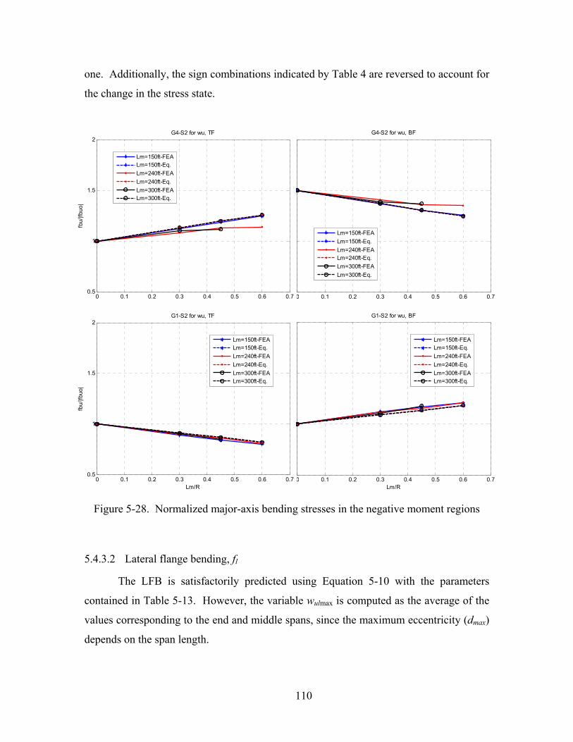
110
one. Additionally, the sign combinations indicated by Table 4 are reversed to account for
the change in the stress state.
0 0.1 0.2 0.3 0.4 0.5 0.6 0.70.5
1
1.5
2G4-S2 for wu, TF
fbu/
|fbuo
|
Lm=150ft-FEALm=150ft-Eq.Lm=240ft-FEALm=240ft-Eq.Lm=300ft-FEALm=300ft-Eq.
0 0.1 0.2 0.3 0.4 0.5 0.6 0.7
G4-S2 for wu, BF
Lm=150ft-FEALm=150ft-Eq.Lm=240ft-FEALm=240ft-Eq.Lm=300ft-FEALm=300ft-Eq.
0 0.1 0.2 0.3 0.4 0.5 0.6 0.70.5
1
1.5
2G1-S2 for wu, TF
fbu/
|fbuo
|
Lm/R
Lm=150ft-FEALm=150ft-Eq.Lm=240ft-FEALm=240ft-Eq.Lm=300ft-FEALm=300ft-Eq.
0 0.1 0.2 0.3 0.4 0.5 0.6 0.7
G1-S2 for wu, BF
Lm/R
Lm=150ft-FEALm=150ft-Eq.Lm=240ft-FEALm=240ft-Eq.Lm=300ft-FEALm=300ft-Eq.
Figure 5-28. Normalized major-axis bending stresses in the negative moment regions
5.4.3.2 Lateral flange bending, fl
The LFB is satisfactorily predicted using Equation 5-10 with the parameters
contained in Table 5-13. However, the variable wulmax is computed as the average of the
values corresponding to the end and middle spans, since the maximum eccentricity (dmax)
depends on the span length.

111
Table 5-13. Fitting parameters for the negative moment regions 150ft 240ft 300ft
d D
(ftd-2) d
D
(ftd-2) d
D
(ftd-2)
G4 1.84 21.52 1.63 10.17 1.52 5.73
G1 1.72 12.93 1.69 12.18 1.36 3.76
Figure 5-29 (including the Figures in Appendix B) shows that the proposed
equations predict satisfactorily the bending effects in both exterior girders, while the code
equations are over conservative for most cases. It is also observed that the LFB in these
regions is practically unaffected by the curvature.
20 25 30 35 40 450
10
20
30
40
50
60
70
80
90
100G4 CV-S2 for wu, TF
Mla
t/wul
max
(ft2 )
L/R=0.30-FEAL/R=0.30-Code Mu-FEAL/R=0.30-Code Mu-Eq.L/R=0.45-FEAL/R=0.45-Code Mu-FEAL/R=0.45-Code Mu-EqL/R=0.60-FEAL/R=0.60-Code Mu-FEAL/R=0.60-Code Mu-Eq.Proposed Eq.
20 25 30 35 40 45
G4 CV-S2 for wu, BF
L/R=0.30-FEAL/R=0.30-Code Mu-FEAL/R=0.30-Code Mu-Eq.L/R=0.45-FEAL/R=0.45-Code Mu-FEAL/R=0.45-Code Mu-EqL/R=0.60-FEAL/R=0.60-Code Mu-FEAL/R=0.60-Code Mu-Eq.Proposed Eq.
15 20 25 30 35 40 450
10
20
30
40
50
60
70
80
90
100G1 CV-S2 for wu, TF
Mla
t/wul
max
(ft2 )
Lb (ft)
L/R=0.30-FEAL/R=0.30-Code Mu-FEAL/R=0.30-Code Mu-Eq.L/R=0.45-FEAL/R=0.45-Code Mu-FEAL/R=0.45-Code Mu-EqL/R=0.60-FEAL/R=0.60-Code Mu-FEAL/R=0.60-Code Mu-Eq.Proposed Eq.
5 20 25 30 35 40 45
G1 CV-S2 for wu, BF
Lb (ft)
L/R=0.30-FEAL/R=0.30-Code Mu-FEAL/R=0.30-Code Mu-Eq.L/R=0.45-FEAL/R=0.45-Code Mu-FEAL/R=0.45-Code Mu-EqL/R=0.60-FEAL/R=0.60-Code Mu-FEAL/R=0.60-Code Mu-Eq.Proposed Eq.
Figure 5-29. LFB in the negative moment regions (Lm=150ft)

112
5.5 Concluding remarks
The bending stresses during the deck placement in straight, skewed and curved
steel I-girder bridges were evaluated using the results obtained from the parametric study
described in Chapter 4. The LFB stresses caused by distributed and concentrated
overhang loads were estimated finding the curves that have the best fit to the critical
stresses obtained from the parametric study. According to this evaluation, the following
major observations were made.
5.5.1 Straight structures
The major-axis bending stresses exhibited by the exterior girders of straight
bridges are independent of the cross-frame spacing. Therefore, these stresses may be
obtained from the structural analysis of either a simplified model that does not consider
explicitly the cross frames or a more detailed model involving any cross-frame distance.
For the positive moment regions, the LFB due to distributed loads was
satisfactorily predicted by the equation proposed in this work over the entire range of
cross-frame distances, principally at the end spans. Although the LFB obtained in the
middle span is lower, the same equations were proposed to simplify the approximations.
Comparisons with the code estimations showed that the Specifications are highly
conservative in all cases, especially for large cross-frame distances.
For concentrated loads, a linear regression considering the most external points
from the critical curves was performed to adjust the numerical stresses. These external
points correspond to models where the concentrated loads are placed at the middle of a
cross-frame spacing which is the critical location. The proposed equation for the bottom
flange governs over the code equation for cross-frame distances larger than 26ft.
However, both the code and the proposed approximations coincide for the top flange.
The LFB effect on the negative moment regions was approximated considering
only the distributed loading case since the contribution from the concentrated loads is
negligible. The results showed that the proposed equation satisfactorily predicts the LFB
in both flanges.

113
5.5.2 Skewed structures
The results showed that skewed bridges exhibit LFB even when torsional loads
are not applied. However, in the presence of torsional effects, the LFB effect is slightly
more pronounced when the cross frames are oriented parallel to the supports. Therefore,
a perpendicular orientation of the cross frames is recommended for general skewed
bridges to increase the lateral stiffness of the structure. This perpendicular configuration
was adopted in this work to evaluate the LFB effects.
The results indicated that the major-axis bending in skewed bridges is not only
independent of the cross-frame spacing but also of the skew angle. Therefore, these
stresses may be taken from structural analyses performed for skewed bridges with any
cross-frame spacing and skew angle, including their simplified straight counterpart.
The LFB in the positive moment regions was approximated using curve fitting
models similar to the ones used for straight bridges. For distributed loads, a lower limit
was introduced in the proposed equation for the bottom flange since this flange exhibits
LFB even for closely spaced cross frames. The minimum LFB stress considered in the
bottom flange is proportional to the skew angle. The results were compared to the code
equation for overhang loads and significant overestimates of the LFB were found
principally for long cross-frame distances.
On the other hand, for concentrated loads, the results showed that the code
equation for overhang loads fails to predict satisfactorily the LFB in most of the cases,
principally in the bottom flange.
The LFB in the negative moment regions was approximated in this work by a
constant term that depends on the skew angle. This approximation was adopted to
conservatively estimate the stresses which do not exhibit a consistent trend in these
regions. The results also indicated that the code recommendation of using 10Ksi for the
unfactored LFB stresses in skewed bridges is conservative even compared to factored
stresses.

114
5.5.3 Curved structures
The evaluation of the bending stresses in curved bridges indicated that fbu and fl
are deeply affected by the curvature and the position of the girder, i.e. outer or inner
girder.
The analyses showed that the major-bending stresses in curved bridges are
independent of the cross-frame spacing. However, they increase linearly with the
curvature in the positive moment regions of the end spans. Conversely, these stresses at
the middle span of the outer girder are not significantly affected by the curvature.
Therefore, a linear model was proposed to estimate the major-bending effects in the
positive moment regions of both exterior girders. This model computes the major-axis
bending in curved bridges based on the major-axis bending stresses exhibited by their
straight counterpart. Therefore, the proposed equation allows estimating fbu in curved
bridges from structural analyses of simplified straight bridges. In the negative moment
regions, the major-bending stresses also exhibit a linear trend but it is independent of the
span length.
The assumption of computing fbu based on a simplified model with the real arc
length of the curved girder does not help to represent the curvature effects on fbu. In fact,
the AASHTO recommendation of ignoring the curvature effects for fbu when L/R is lower
than 0.06 introduces an error of approximately 10% in long span bridges.
The LFB in curved girders is caused by both the curvature and the overhang
loads. However, it was shown that the participation of the overhang loads in the LFB is
low compared to the curvature effects. In fact, the overhang-to-curvature effect ratio
reduces as the length of the span and the curvature increase. Therefore, the overhang
term was dropped from the final expression proposed for the LFB which simplifies to the
curvature term only. However, the torsional effects due to overhang loads are implicitly
considered since the curve fitting process is applied to the total LFB obtained from the
parametric study. A comprehensive formulation to estimate the LFB effects due to
curvature was developed for distributed and concentrated loads, respectively. The critical
case between the top and bottom flanges was selected to define the equations proposed in
this work to estimate the LFB in curved bridges.

115
The results indicated that the LFB is practically unaffected by the variation of the
curvature, a slight effect was only observed in the positive moment regions of the middle
span. This observation indicates that these effects need to be considered even in bridges
with large curvature radii.
The equations proposed in this project to estimate the LFB in curved bridges work
adequately in both exterior girders. Significant reductions were found in most of the
cases compared to the estimations given by the AASHTO Specifications.
The major-axis bending effects in the AASHTO equation were computed using
both the numerical and the estimated major-axis bending stresses, obtaining similar
results. The estimated major-axis bending stresses correspond to the stresses computed
using the equation proposed in this work to estimate fbu in curved bridges from the results
obtained in their straight counterpart. Therefore, the LFB in a curved bridge can be
conservatively approximated using the code equation together with the major-axis
bending from the corresponding straight bridge. The advantage of the proposed
equations over the code approximation is that it is not required to know in advance the
major-bending effects to compute the LFB. However, the principal disadvantage is that
different expressions are required to define the effects of distributed and concentrated
loads, while the code approximation consists of one single equation that applies for all
load cases independent of the girder location and flange position.
However, the results from the parametric study indicated that the code equation
fails to predict the LFB due to distributed loads at the inner girder of highly curved
bridges with long spans. Therefore, it is recommended to use the equation proposed in
this work which predicts satisfactorily the LFB in all cases. It was also observed that the
bottom flange under concentrated loads exhibits the most critical LFB effects compared
to the top flange, especially for short span lengths.
The results indicated that the outer girder exhibits the most critical combined
bending effects. On the contrary, the curvature decreases the magnitude of the major-
bending stresses in the inner girder resulting in a combined bending action much lower
than that corresponding to the outer girder. Therefore, the design of both exterior girders
shall be based on the evaluation of the outer girder, unless an optimization of the inner

116
girder is pursued. In that case, the effects of the girder stiffness in the behavior of the
whole cross section of the deck shall be investigated.
In general, it is recommended to distribute the cross frames such that a cross
frame is placed at the maximum vertical bending moment to decrease the combined
effect of fl and fbu during construction.

117
Chapter 6: Evaluation of the flexural limit states for constructibility
In this chapter, the flexural limit states for constructibility are evaluated according
to AASHTO Specifications for the parametric bridges analyzed in this work.
First, the major-axis bending and the LFB stresses obtained from FEA are used to
evaluate the demand-to-capacity ratios of the flexural limit states for constructibility.
This evaluation allows identifying the critical sections along the bridge and the effects of
the cross-frame spacing and the deck-placement sequence in the governing limit states.
Second, the maximum allowable skews and curvatures are computed for bridges
designed originally as straight. The flexural limit states for constructibility constitute the
criteria used to achieve this goal. The major-axis bending stresses are taken directly from
FEA and the LFB stresses are estimated using the approximate equations proposed in
Chapter 5.
6.1 General observations
The bending results from FEA were evaluated using the flexural limit state
equations for constructibility. These limit states are applied in a normalized form
(demand-over-capacity) as follows:
• Discretely braced flanges in compression:
Yielding: 1bu l
f h yc
f fR Fφ
+≤ 6-1
Ultimate strength:
13 1
bu l
f nc
f f
Fφ
+≤ 6-2
Web bend-buckling: 1bu
f crw
fFφ
≤ 6-3
• Discretely braced flanges in tension:
Yielding: 1bu l
f h yt
f fR Fφ
+≤ 6-4

118
• Continuously braced flanges in tension or compression:
Yielding: 1bu
f h yf
fR Fφ
≤ 6-5
Limit for LFB: 10.6
l
yf
fF
≤ 6-6
In the following sections, the limit state ratios of the skewed and the curved
bridges are compared to the results obtained from their straight counterparts.
6.1.1 Skewed bridges
For the skewed bridge configurations analyzed in this work, it is observed that the
effect on the limit state ratios of the girder position, the cross-frame orientation and the
skew angle is almost negligible as shown in Figure 6-1. However, the cross-frame
spacing has a significant effect on the limit state ratios of discretely braced flanges in
compression in the positive moment regions, since the LFB depends on Lb and the
capacity of the flange is reduced as Lb increases.
Although the limit state ratios are not visibly affected by the skew, the proposed
equations for the LFB presented in Chapter 5 are intended to represent the maximum
possible variations on fl caused by the skewed geometry of the structure.
Figure 6-2 (see other figures in Appendix C) also shows that sections S1 and S3
are controlled by the second and fourth castings, respectively. The corresponding flanges
in compression in both sections are governed by the ultimate strength limit state.
The negative moment regions are controlled by the fifth casting stage. The
flanges in compression are governed by the yielding limit state when the span lengths are
short. However, the web bend-buckling limit state governs the compression flanges for
long span lengths.

119
G4 - XF1 - Lb=25ft G1 - XF1 – Lb=25ft
0 0.05 0.1 0.15 0.2 0.25 0.3 0.35 0.4 0.45 0.5
-0.5
-0.4
-0.3
-0.2
-0.1
0
0.1
0.2
0.3
0.4
0.5
Dem
and/
Cap
acity
0 0.05 0.1 0.15 0.2 0.25 0.3 0.35 0.4 0.45 0.5
G4 -XF1 - Lb=40ft G4 - XF2 - Lb=40ft
0 0.05 0.1 0.15 0.2 0.25 0.3 0.35 0.4 0.45 0.5
-0.5
-0.4
-0.3
-0.2
-0.1
0
0.1
0.2
0.3
0.4
0.5
Normalized distance (xi/Lt)
Dem
and/
Cap
acity
0 0.05 0.1 0.15 0.2 0.25 0.3 0.35 0.4 0.45 0.5Normalized distance (xi/Lt)
Figure 6-1. Variation of the limit state ratios along the length of skewed bridges
TF: ST L/R=0.30 L/R=0.45 L/R=0.60
BF: ST L/R=0.30 L/R=0.45 L/R=0.60

120
25 27 32 370
0.2
0.4
0.6
0.8
1
1.2
G4 Lm=150ft, TF S1D
/C m
ax
25 27 32 370
1
2
3
4
5
Cas
ting
#
25 27 32 370
1
2
3
4
5
Lb (ft)
Lim
it S
tate
ST SK30 SK45 SK60
25 27 32 37
G4 Lm=150ft, BF S1
25 27 32 37
25 27 32 37Lb (ft)
ST SK30 SK45 SK60
20 21 27 350
0.2
0.4
0.6
0.8
1
1.2
G4 Lm=150ft, TF S2
D/C
max
20 21 27 350
1
2
3
4
5
Cas
ting
#
20 21 27 350
1
2
3
4
5
Lb (ft)
Lim
it S
tate
ST SK30 SK45 SK60
20 21 27 35
G4 Lm=150ft, BF S2
20 21 27 35
20 21 27 35Lb (ft)
ST SK30 SK45 SK60
Figure 6-2. Effect of parametric variables in the limit states of skewed bridges

121
22 27 32 400
0.2
0.4
0.6
0.8
1
1.2
G4 Lm=150ft, TF S3D
/C m
ax
22 27 32 400
1
2
3
4
5
Cas
ting
#
22 27 32 400
1
2
3
4
5
Lb (ft)
Lim
it S
tate
ST SK30 SK45 SK60
22 27 32 40
G4 Lm=150ft, BF S3
22 27 32 40
22 27 32 40Lb (ft)
ST SK30 SK45 SK60
Figure 6-2. Effect of parametric variables in the limit states of skewed bridges (Cont.)
6.1.2 Curved bridges
Figure 6-3 illustrates that both the curvature and the cross-frame spacing highly
affect the limit state ratios in the outer girder principally in the positive moment regions,
while a stress relief is observed in the inner girder. This is caused by the length
adjustments due to curvature since interior girders shorten as the curvature increases
generating lower major-axis bending stresses. The opposite situation occurs in the outer
girders where the vertical stresses increase. Additionally, the LFB exhibited by the inner
girder is relieved since its eccentricity with respect to the supports is smaller.
In fact, the LFB undergoes a reversal effect in the inner girder compared to its
straight counterpart, as shown in Figure 6-4. This is due to the curvature and overhang
loading torsional effects counteracting each other in the inner girder. However, the
curvature effects govern over the torsion produced by the overhang loads.

122
Lb =25ft
0 0.05 0.1 0.15 0.2 0.25 0.3 0.35 0.4 0.45 0.5
-1
-0.8
-0.6
-0.4
-0.2
0
0.2
0.4
0.6
0.8
1
G4 Lm=150ft, C2
Dem
and/
Cap
acity
0 0.05 0.1 0.15 0.2 0.25 0.3 0.35 0.4 0.45 0.5
G1 Lm=150ft, C2
Lb =40ft
0 0.05 0.1 0.15 0.2 0.25 0.3 0.35 0.4 0.45 0.5
-1
-0.8
-0.6
-0.4
-0.2
0
0.2
0.4
0.6
0.8
1
G4 Lm=150ft, C2
Normalized distance (xi/Lt)
Dem
and/
Cap
acity
0 0.05 0.1 0.15 0.2 0.25 0.3 0.35 0.4 0.45 0.5
G1 Lm=150ft, C2
Normalized distance (xi/Lt)
Figure 6-3. Variation of the limit state ratios along the length of curved bridges
TF: ST L/R=0.30 L/R=0.45 L/R=0.60
BF: ST L/R=0.30 L/R=0.45 L/R=0.60

123
0 0.05 0.1 0.15 0.2 0.25 0.3 0.35 0.4 0.45 0.5
-0.6
-0.4
-0.2
0
0.2
0.4
0.6
G4 Lm=150ft, C2, TF
Normalized distance (xi/Lt)
fl / F
yf
0 0.05 0.1 0.15 0.2 0.25 0.3 0.35 0.4 0.45 0.5
G1 Lm=150ft, C2, TF
Normalized distance (xi/Lt)
Figure 6-4. Variation of the LFB along the length of curved bridges
Figure 6-5, Figure 6-6 and Figure 6-7 show that the cross-frame spacing affects
the limit state ratios in the outer girders as well. It is also observed that second and fourth
castings from the deck-placement sequence control sections S1 and S3, respectively.
Compression flanges in these sections are governed by the ultimate strength limit state.
However, the yielding limit state may control in short span lengths with high curvatures.
As for skewed bridges, the negative moment regions are controlled by the fifth
casting stage. The yielding limit state governs the compression flanges of bridges with
short spans and the web bend-buckling limit state becomes significant in the pier regions
for long span bridges (see Figures in Appendix D).
ST
L/R=0.30
L/R=0.45
L/R=0.60

124
25 27 32 370
0.2
0.4
0.6
0.8
1
1.2
G4 Lm=150ft, TF S1D
/C m
ax
25 27 32 370
1
2
3
4
5
Cas
ting
#
25 27 32 370
1
2
3
4
5
Lb (ft)
Lim
it S
tate
ST CV30 CV45 CV60
25 27 32 37
G4 Lm=150ft, BF S1
25 27 32 37
25 27 32 37Lb (ft)
ST CV30 CV45 CV60
25 27 32 370
0.2
0.4
0.6
0.8
1
1.2
G1 Lm=150ft, TF S1
D/C
max
25 27 32 370
1
2
3
4
5
Cas
ting
#
25 27 32 370
1
2
3
4
5
Lb (ft)
Lim
it S
tate
ST CV30 CV45 CV60
25 27 32 37
G1 Lm=150ft, BF S1
25 27 32 37
25 27 32 37Lb (ft)
ST CV30 CV45 CV60
Figure 6-5. Effect of parametric variables in the limit state ratios of Section S1

125
20 21 27 350
0.2
0.4
0.6
0.8
1
1.2
G4 Lm=150ft, TF S2D
/C m
ax
20 21 27 350
1
2
3
4
5
Cas
ting
#
20 21 27 350
1
2
3
4
5
Lb (ft)
Lim
it S
tate
ST CV30 CV45 CV60
20 21 27 35
G4 Lm=150ft, BF S2
20 21 27 35
20 21 27 35Lb (ft)
ST CV30 CV45 CV60
20 21 27 350
0.2
0.4
0.6
0.8
1
1.2
G1 Lm=150ft, TF S2
D/C
max
20 21 27 350
1
2
3
4
5
Cas
ting
#
20 21 27 350
1
2
3
4
5
Lb (ft)
Lim
it S
tate
ST CV30 CV45 CV60
20 21 27 35
G1 Lm=150ft, BF S2
20 21 27 35
20 21 27 35Lb (ft)
ST CV30 CV45 CV60
Figure 6-6. Effect of parametric variables in the limit state ratios of Section S2

126
22 27 32 400
0.2
0.4
0.6
0.8
1
1.2
G4 Lm=150ft, TF S3D
/C m
ax
22 27 32 400
1
2
3
4
5
Cas
ting
#
22 27 32 400
1
2
3
4
5
Lb (ft)
Lim
it S
tate
ST CV30 CV45 CV60
22 27 32 40
G4 Lm=150ft, BF S3
22 27 32 40
22 27 32 40Lb (ft)
ST CV30 CV45 CV60
22 27 32 400
0.2
0.4
0.6
0.8
1
1.2
G1 Lm=150ft, TF S3
D/C
max
22 27 32 400
1
2
3
4
5
Cas
ting
#
22 27 32 400
1
2
3
4
5
Lb (ft)
Lim
it S
tate
ST CV30 CV45 CV60
22 27 32 40
G1 Lm=150ft, BF S3
22 27 32 40
22 27 32 40Lb (ft)
ST CV30 CV45 CV60
Figure 6-7. Effect of parametric variables in the limit state ratios of Section S3

127
6.2 Maximum allowable skew angle and curvature for straight bridges
during construction
In this section, the straight bridge models are evaluated using the flexural limit
states for constructibility in order to define the maximum allowable skew angles and
curvatures for the loading conditions given during deck placement. This evaluation will
provide the engineer with design information for curved and skewed bridges based on
their straight girder counterparts. Furthermore, no additional constructibility designs or
checks would be necessary in case that a bridge designed as straight requires a
geometrical modification within the limits established.
To achieve this goal, the maximum cross-frame spacing (Lb max) was computed for
each straight bridge considered in this work from the limit state equations for
constructibility that directly depend on Lb (Eqns. 6-1, 6-2, 6-4 and 6-6). In the limit state
equations, the major-axis bending effects were taken from FEA and the LFB stresses
were expressed in terms of Lb using the approximate equations recommended in Chapter
5 for straight bridges. After finding Lb max by solving the critical limit state equation, the
maximum skew angle and curvature are computed for different Lb values based on the
limit state equations for constructibility as well.
6.2.1 Skew angle
The maximum skew was computed by solving the limit state equations for each
Lb value. However, the LFB in these equations are expressed in terms of Lba/A or Lb/B+C
for distributed and concentrated loads in the positive moment regions, respectively.
Therefore, these terms are solved from the limit state equations and then are compared to
the corresponding values defined in Chapter 5 for θ=30°, 45° and 60° as shown in Figure
6-8, Figure 6-9 and Figure 6-10 for Lm=150ft, 240ft and 300ft, respectively. For the
negative moment regions, the comparisons are established in terms of stresses.
It is observed that the maximum cross-frame spacing in skewed bridges is
controlled by the ultimate strength limit state in the compression flange (Eq. 6-2).
Conversely, the tension flange seems to be unaffected by the skew angle.

128
25 30 35 40 45 50 550
50
100
150
200
250
300
350
Lba /A
(ft2 )
Postive Moment Region - Top Flange - Lm=150ft
θ=30o
θ=45o
θ=60o
S1-maxS3-max
25 30 35 40 45 50
1
2
3
4
5
6
(f )
Lim
it S
tate
Postive Moment Region - Top Flange - Lm=150ft
S1-maxS3-max
25 30 35 40 45 50 550
50
100
150
200
250
300
350
Lba /A
(ft2 )
Postive Moment Region - Bottom Flange - Lm=150ft
θ=30o
θ=45o
θ=60o
S1-maxS3-max
25 30 35 40 45 50
1
2
3
4
5
6
Lim
it S
tate
Postive Moment Region - Bottom Flange - Lm=150ft
S1-maxS3-max
25 30 35 40 45 50 550
5
10
15
20
25
30
Lb (ft)
fl m
ax (K
si)
Negative Moment Region - Lm=150ft
θ=30o
θ=45o
θ=60o
S2-TFS2-BF
25 30 35 40 45 50
1
2
3
4
5
6
Lb (ft)
Lim
it S
tate
Negative Moment Region - Lm=150ft
S2-TFS2-BF
Figure 6-8. Identification of maximum skew angles for straight bridges with Lm=150ft

129
25 30 35 40 45 50 55 60 65 70 750
100
200
300
400
500
600
700
800Lb
a /A (f
t2 )Postive Moment Region - Top Flange - Lm=240ft
θ=30o
θ=45o
θ=60o
S1-maxS3-max
25 30 35 40 45 50 55 60
1
2
3
4
5
6
Lim
it S
tate
Postive Moment Region - Top Flange - Lm=240ft
S1-maxS3-max
25 30 35 40 45 50 55 60 65 70 750
100
200
300
400
500
600
700
800
Lba /A
(ft2 )
Postive Moment Region - Bottom Flange - Lm=240ft
θ=30o
θ=45o
θ=60o
S1-maxS3-max
25 30 35 40 45 50 55 60
1
2
3
4
5
6
Lim
it S
tate
Postive Moment Region - Bottom Flange - Lm=240ft
S1-maxS3-max
25 30 35 40 45 50 55 60 65 70 750
5
10
15
20
25
30
Lb (ft)
fl m
ax (K
si)
Negative Moment Region - Lm=240ft
θ=30o
θ=45o
θ=60o
S2-TFS2-BF
25 30 35 40 45 50 55 60 65 70
1
2
3
4
5
6
Lb (ft)
Lim
it S
tate
Negative Moment Region - Lm=240ft
S2-TFS2-BF
Figure 6-9. Identification of maximum skew angles for straight bridges with Lm=240ft

130
20 30 40 50 60 70 800
100
200
300
400
500
600
700
800
900
1000Lb
a /A (f
t2 )Postive Moment Region - Top Flange - Lm=300ft
θ=30o
θ=45o
θ=60o
S1-maxS3-max
25 30 35 40 45 50 55 60 65 70
1
2
3
4
5
6
Lim
it S
tate
Postive Moment Region - Top Flange - Lm=300ft
S1-maxS3-max
20 30 40 50 60 70 800
100
200
300
400
500
600
700
800
900
1000
Lba /A
(ft2 )
Postive Moment Region - Bottom Flange - Lm=300ft
θ=30o
θ=45o
θ=60o
S1-maxS3-max
25 30 35 40 45 50 55 60 65 70
1
2
3
4
5
6
Lim
it S
tate
Postive Moment Region - Bottom Flange - Lm=300ft
S1-maxS3-max
20 30 40 50 60 70 800
5
10
15
20
25
30
Lb (ft)
fl m
ax (K
si)
Negative Moment Region - Lm=300ft
θ=30o
θ=45o
θ=60o
S2-TFS2-BF
25 30 35 40 45 50 55 60 65 70 75
1
2
3
4
5
6
Lb (ft)
Lim
it S
tate
Negative Moment Region - Lm=300ft
S2-TFS2-BF
Figure 6-10. Identification of maximum skew angles for straight bridges with Lm=300ft

131
6.2.2 Curvature
For curved bridges, both fbu and fl depend on the curvature as indicated by the
approximate equations proposed in Chapter 5. The maximum curvature L/R is solved
from the limit state equations for different Lb values as shown in Figure 6-11, Figure 6-12
and Figure 6-13 for Lm=150ft, 240ft and 300ft, respectively. It is noticed that the
maximum curvature is controlled by the end-span cross section in the outer girder. In
addition, it is also shown that the ultimate strength limit state of the compression flange
controls the maximum allowable curvature for high Lb values.
The code specifies a maximum cross frame spacing for curved bridges as follows:
( )
max
max
0.1 0.1/
/ 0.1
b
b
LL RL RLL RL
= =
∴ = 6-7
where R is the radius of curvature. Comparisons with the numerical results show that the
code recommendation of L/R is adequate in short span bridges (150ft) when Lb is less
than 40ft approximately. However, long span bridges present an allowable curvature
lower than the one recommended in the code when the cross sections are designed from a
straight girder formulation.
25 30 35 40 45 500
0.5
1
1.5
2
2.5
3
L/R
G4- Top Flange - Lm=150ft
S1S2S3Code-S1Code-S3
25 30 35 40 45 50
1
2
3
4
5
6
LS
G4- Top Flange - Lm=150ft
S1S2S3

132
25 30 35 40 45 500
0.5
1
1.5
2
2.5
3L/
RG4-Bottom Flange - Lm=150ft
S1S2S3Code-S1Code-S3
25 30 35 40 45 50
1
2
3
4
5
6
LS
G4- Bottom Flange - Lm=150ft
S1S2S3
25 30 35 40 45 500
0.5
1
1.5
2
2.5
3
L/R
G1- Top Flange - Lm=150ft
S1S2S3Code-S1Code-S3
25 30 35 40 45 50
1
2
3
4
5
6
LS
G1- Top Flange - Lm=150ft
S1S2S3
25 30 35 40 45 500
0.5
1
1.5
2
2.5
3
Lb (ft)
L/R
G1- Bottom Flange - Lm=150ft
S1S2S3Code-S1Code-S3
25 30 35 40 45 50
1
2
3
4
5
6
Lb (ft)
LS
G1- Bottom Flange - Lm=150ft
S1S2S3
Figure 6-11. Identification of maximum curvatures for straight bridges with Lm=150ft

133
25 30 35 40 45 50 55 60 65 700
0.5
1
1.5
2
2.5
3L/
RG4- Top Flange - Lm=240ft
S1S2S3Code-S1Code-S3
25 30 35 40 45 50 55 60 65 70
1
2
3
4
5
6
LS
G4- Top Flange - Lm=240ft
S1S2S3
25 30 35 40 45 50 55 60 65 700
0.5
1
1.5
2
2.5
3
L/R
G4-Bottom Flange - Lm=240ft
S1S2S3Code-S1Code-S3
25 30 35 40 45 50 55 60 65 70
1
2
3
4
5
6
LS
G4- Bottom Flange - Lm=240ft
S1S2S3
25 30 35 40 45 50 55 60 65 700
0.5
1
1.5
2
2.5
3
Lb (ft)
L/R
G1- Top Flange - Lm=240ft
S1S2S3Code-S1Code-S3
25 30 35 40 45 50 55 60 65 70
1
2
3
4
5
6
Lb (ft)
LS
G1- Top Flange - Lm=240ft
S1S2S3

134
25 30 35 40 45 50 55 60 65 700
0.5
1
1.5
2
2.5
3
Lb (ft)
L/R
G1- Bottom Flange - Lm=240ft
S1S2S3Code-S1Code-S3
25 30 35 40 45 50 55 60 65 70
1
2
3
4
5
6
Lb (ft)
LS
G1- Bottom Flange - Lm=240ft
S1S2S3
Figure 6-12. Identification of maximum curvatures for straight bridges with Lm =240ft
25 30 35 40 45 50 55 60 65 70 750
0.5
1
1.5
2
2.5
3
L/R
G4- Top Flange - Lm=300ft
S1S2S3Code-S1Code-S3
25 30 35 40 45 50 55 60 65 70 75
1
2
3
4
5
6
LSG4- Top Flange - Lm=300ft
S1S2S3
25 30 35 40 45 50 55 60 65 70 750
0.5
1
1.5
2
2.5
3
Lb (ft)
L/R
G4-Bottom Flange - Lm=300ft
S1S2S3Code-S1Code-S3
25 30 35 40 45 50 55 60 65 70 75
1
2
3
4
5
6
Lb (ft)
LS
G4- Bottom Flange - Lm=300ft
S1S2S3

135
25 30 35 40 45 50 55 60 65 70 750
0.5
1
1.5
2
2.5
3L/
RG1- Top Flange - Lm=300ft
S1S2S3Code-S1Code-S3
25 30 35 40 45 50 55 60 65 70 75
1
2
3
4
5
6
LS
G1- Top Flange - Lm=300ft
S1S2S3
25 30 35 40 45 50 55 60 65 70 750
0.5
1
1.5
2
2.5
3
Lb (ft)
L/R
G1- Bottom Flange - Lm=300ft
S1S2S3Code-S1Code-S3
25 30 35 40 45 50 55 60 65 70 75
1
2
3
4
5
6
Lb (ft)
LS
G1- Bottom Flange - Lm=300ft
S1S2S3
Figure 6-13. Identification of maximum curvatures for straight bridges with Lm =300ft
6.3 Concluding remarks
In the first part of this chapter, the behavior of the limit states for constructibility
were evaluated based on the FEA results obtained from the parametric study. The
following major conclusions were made.
For the skewed bridges analyzed in this work, it was observed that the effect on
the limit states of the girder position, the cross-frame orientation and the skew angle is
almost negligible. However, the cross-frame spacing has a significant effect on the limit
state of discretely braced flanges in compression principally in the positive moment

136
regions, since the LFB depends on the cross-frame distance and the capacity of the flange
reduces as this parameter increases.
It was also observed that the cross sections at the positive moment regions of the
end and middle spans are controlled by the second and fourth castings, respectively. The
corresponding flanges in compression in both sections are governed by the ultimate
strength limit state. The negative moment regions are controlled by the fifth casting
stage. The flanges in compression are governed by the yielding limit state for short span
lengths bridges. However, the web bend-buckling limit state governs the compression
flanges for longer spans.
In curved bridges, the results showed that both the curvature and the cross-frame
spacing highly affect the limit state ratios in the positive moment regions of the outer
girder. However, a stress relief was observed in the inner girder caused by the length
adjustments due to curvature. Additionally, the LFB exhibited by the inner girder is
relieved since its eccentricity with respect to the supports is smaller. In fact, the LFB
undergoes a reversing effect in the inner girder compared to its straight counterpart. This
is caused from the torsional effects that are controlled by the curvature counteracting the
overhang load effects in the inner girder.
It was observed that the variables that most affect the limit states are the curvature
followed by the cross-frame spacing. The second and fourth castings from the deck-
placement sequence control the sections at the positive moment regions of the end and
middle spans, respectively. The ultimate strength is the limit state that principally
governs the compression flanges in these sections. However, the yielding limit state may
control in short span lengths with high curvatures.
As for skewed bridges, the negative moment regions are controlled by the fifth
casting stage. The yielding limit state governs the compression flanges of bridges with
short spans and the web bend-buckling limit state becomes significant in the pier regions
for long span bridges.
None of the critical limit state values resulted from a casting stage where the
finishing machine is considered.

137
In the second part of Chapter 6, the maximum allowed skews and curvatures were
computed for straight bridges based on the limit states for constructibility and the LFB
equations proposed in Chapter 5. The following principal observations were established.
For skewed bridges, it was observed that the maximum cross-frame spacing in
skewed bridges is controlled by the ultimate strength limit state in the compression
flange. Conversely, the tension flange seems to be unaffected by the skew angle.
On the other hand, the maximum allowed curvature is controlled in most of the
cases by the end-span cross section in the outer girder. It was also shown that the
ultimate strength limit state of the compression flange controls the maximum allowable
curvature for large cross-frame distances. Comparisons with the code recommendation
about the maximum cross-frame spacing in curved bridges showed that this specification
is adequate in short span bridges when the distance between cross frames is less than
approximately 40ft. However, long span bridges present an allowable curvature lower
than the one recommended in the code when the cross sections are designed from a
straight girder formulation.
138
Chapter 7: Cross-frame spacing optimization
AASHTO (2007) does not include a specific recommendation for the spacing of
cross frames in steel bridges. Therefore, the designer needs to either evaluate different
configurations to select the optimum spacing, or follow traditional practice that assures
safe results. For that reason, a reliability analysis was proposed in this work and
performed in Chapter 7 to develop a practical method to select the cross-frame spacing
for deck placement conditions considering the flexural limit states for constructibility that
are affected by the cross-frame spacing. Initially, a general description of a structural
reliability study is given along with the limit states considered in this work. Then, the
adopted structural loading and resistance models are described and their corresponding
probabilistic characteristics are presented. Finally, a Monte Carlo Simulation is
performed for straight, skewed and curved steel I-girder bridges generating some fragility
curves that allow the maximum cross-frame spacing for deck-placement conditions
according to the maximum tolerated level of risk to be identified.
7.1 Limit States
According to Nowak and Collins (2000), a limit state is the boundary between the
desired and undesired performance of a structure. The definition of a limit state is based
on the identification of a potential structural failure that makes the structure unable to
perform as intended originally in the design, e.g. excessive deflections, exceeding the
moment capacity, buckling. The structural limit states are generally classified as
ultimate, serviceability or fatigue limit states depending on the failure type prevented.
Thus, ultimate limit states correspond to the loss of load-carrying capacity, the
serviceability limit states are related with the user’s comfort and the fatigue limit states
control the loss of strength due to cyclic loads.
Mathematically, the limit states are represented by a performance function,
defined as:
( ),g R Q R Q= − 7-1

139
where, R represents the “capacity or resistance” and Q the “demand”. The limit state is
obtained specifically when g = 0, which is the border between the safe and unsafe zones
as shown in Figure 7-1. If g ≥ 0, the structure is safe, otherwise, an undesired structural
performance is exhibited. The basic variables R and Q are functions of other specific
variables such as load components, influence factors, resistance parameters, material
properties, dimensions, etc. Some of these variables may be of random nature.
Therefore, the failure of the system needs to be addressed probabilistically.
Figure 7-1. Limit State function (Nowak & Collins, 2000)
Random variables are characterized by their probability density function (PDF),
as shown in Figure 7-2 for R and Q. Moreover, R-Q is also a random quantity in which
the probability of failure is represented by the shaded area where the demand exceeds the
capacity. The analytical expression of the probability of failure is given by (Nowak &
Collins, 2000):
( ) ( ) ( ) ( )1f Q i R i i R i Q i iP F r f r dr F q f q dq+∞ +∞
−∞ −∞
= − =∫ ∫ 7-2
where FQ and FR are the Cumulative Distribution Functions (CDF) of Q and R, fQ and fR
are the Probability Density Functions (PDF) of Q and R, and qi and ri are specific values
of Q and R. Since Eq. 7-2 is difficult to evaluate analytically, alternative procedures are
used to indirectly compute the probability of failure based on the concept of the reliability
index.

140
Figure 7-2. Probability functions of load and resistance (Nowak & Collins, 2000)
The reliability index, also known as the safety index, is the ratio of the mean
value of the limit state to its standard deviation, as shown in Figure 7-3. However, a
more common definition is given when the limit state is expressed in terms of the
reduced variables, which are a nondimensional form of the original random variables R
and Q as follows:
RR
R
Q
RZ
QZ
μσ
μσ
−=
−=
7-3
where Z, μ and σ are the reduced variable, the mean value and the standard
deviation, respectively. If R and Q are represented graphically in a space of reduced
variables as shown in Figure 7-4, the reliability index corresponds to the shortest distance
from the origin to the line representing the limit state (g=0). Using equation 7-3 and
geometry, the reliability index is defined as:
22QR
QR
σσ
μμβ
+
−= 7-4
Additionally, if R and Q are normally distributed random variables, the reliability
index is related to the probability of failure by:
( ) ( )ββ −Φ=Φ−= −ff PP or 1 7-5
where Φ is the CDF of a standard normal variable. For random variables
different than normally distributed and uncorrelated variables, equation 7-5 only gives an
approximate definition of β.

141
a. b.
Figure 7-3. Reliability index in: a. general, and b. reduced coordinates (Melchers, 1999)
Figure 7-4. Graphical representation of the Reliability Index (Nowak & Collins, 2000)
The present work evaluates the reliability of the flexural limit states for
constructibility that are directly affected by the cross-frame spacing, i.e. limit states that
consider LFB, as follows:
• Discretely braced flanges in compression:
Yielding: bu l f h ycf f R Fφ+ ≤ 7-6
Ultimate strength: 13bu l f ncf f Fφ+ ≤ 7-7
• Discretely braced flanges in tension:
Yielding: bu l f h ytf f R Fφ+ ≤ 7-8
Limit for LFB: 0.6l yff F≤ 7-9
In order to evaluate the reliability of the limit state equations, it is necessary to
define the probabilistic characteristics of the loading and capacity variables that are

142
involved in the equations. These definitions are called structural loading and resistance
models and are described next.
7.2 Structural loading model
In this work, the demand (fbu, fl) comes from factored loads corresponding to the
Strength-I load combination for construction, where the load factors are taken as 1.25 and
1.5 for the dead and the construction loads, respectively (AASHTO, 2007).
All loading variables are treated as normal random variables. The probabilistic
properties of the dead and construction loads are taken from the work developed by
Nowak et. al. (2006) for the calibration of the LRFD design specifications for steel
curved girder bridges. The bias factors (λ) and coefficients of variation (V) indicated in
Table 7-1 are based on field measurements made by the University of Minnesota.
Table 7-1. General probabilistic characteristics of loads
Bias Factor
(λ)
Coefficient of Variation
(V)
Dead Loads (D) 1.0 0.150
Construction Loads (C) 1.1 0.215
7.2.1 Vertical effects, fbu
7.2.1.1 Definition
Direct vertical loads produce the major-axis bending stress, fbu, in the girder
flanges. In this study, fbu corresponds to the maximum values obtained in the FEA of the
parametric study described in Chapter 4. Because the influence of the cross-frame
spacing in fbu is almost negligible as shown in Chapter 5, fbu is taken only from the FE
models with Lb=25ft.

143
7.2.1.2 Probabilistic characteristics
Because fbu is a total factored stress resulting from the considered load
combination, it is necessary to define λ and V for the total vertical load (TL), as follows:
fbun
TLTL
λ = 7-10
( ) ( )2 2n D D n C C
fbu
D V C VV
TLλ λ+
= 7-11
D n C nTL D Cλ λ= + 7-12
1.25 1.5n n nTL D C= + 7-13
where Xn is the nominal or design value recommended in the specifications for the X load
and X is the corresponding mean value. Table 7-2 contains the values computed for the
exterior girders subjected to distributed vertical loads. The same properties are
considered for concentrated loads, since in this case the construction-to-dead load ratios
are smaller.
Table 7-2. Probabilistic characteristics of distributed vertical loads in exterior girders
Lm (ft) Dn (Kip/ft) Cn(Kip/ft) TLn TL λ fbu V fbu
150 1.45 0.64 2.77 2.16 0.777 0.123
240 1.67 0.64 3.06 2.38 0.779 0.123
300 1.81 0.64 3.23 2.52 0.780 0.123
7.2.2 Torsional effects, fl
7.2.2.1 Definition
Torsional effects generate indirect LFB. In this work, the LFB effects are
computed according to the approximated equations recommended in Chapter 5.
Although these stresses depend directly on the cross-frame spacing, Lb is considered as a
deterministic variable in the reliability analyses and is varied from 15ft to 100ft using 5ft
increments.

144
7.2.2.2 Probabilistic characteristics
An approach similar to the one described for vertical loads is followed to define
the probabilistic characteristics of the lateral factored loads due to eccentric overhang
loading, as shown in Table 7-3. However, the same values contained in Table 7-2 are
used for the curvature effects since the proposed LFB equations for curvature depend on
the vertical loads only.
Table 7-3. Probabilistic characteristics of distributed lateral loads in exterior girders
Lm (ft) Dn (Kip/ft) Cn(Kip/ft) TLn TL λ fl V fl
150 0.17 0.20 0.52 0.40 0.761 0.137
240 0.13 0.15 0.38 0.29 0.761 0.137
300 0.12 0.14 0.37 0.28 0.761 0.137
7.3 Structural resistance model
7.3.1 Definition
In the limit states described in Section 7.1, the resistance R corresponds to the
right side of the inequalities given by Equations 7-3, 7-4, 7-5 and 7-6. The resistance
factor, φf, is taken as 1.0 for flexure and Rh is 1.0 for homogenous girders (AASHTO,
2007). The resistances Fyc, Fyt and Fyf correspond to the specified minimum yield strength
of a compression, tension or any-stress-state flange, respectively. According to the
material properties, these resistances are equal to 50ksi.
On the other hand, Fnc is the nominal flexural resistance of a compression flange.
This resistance is governed by the most critical failure mode between the lateral torsional
buckling (LTB) and the flange local buckling (FLB). The definition of these resistances
is given below according to AASHTO (2007).
7.3.1.1 Lateral Torsional Buckling Resistance:
The lateral torsional buckling resistance of the compression flange is defined as:
• If Lb ≤ Lp, then:
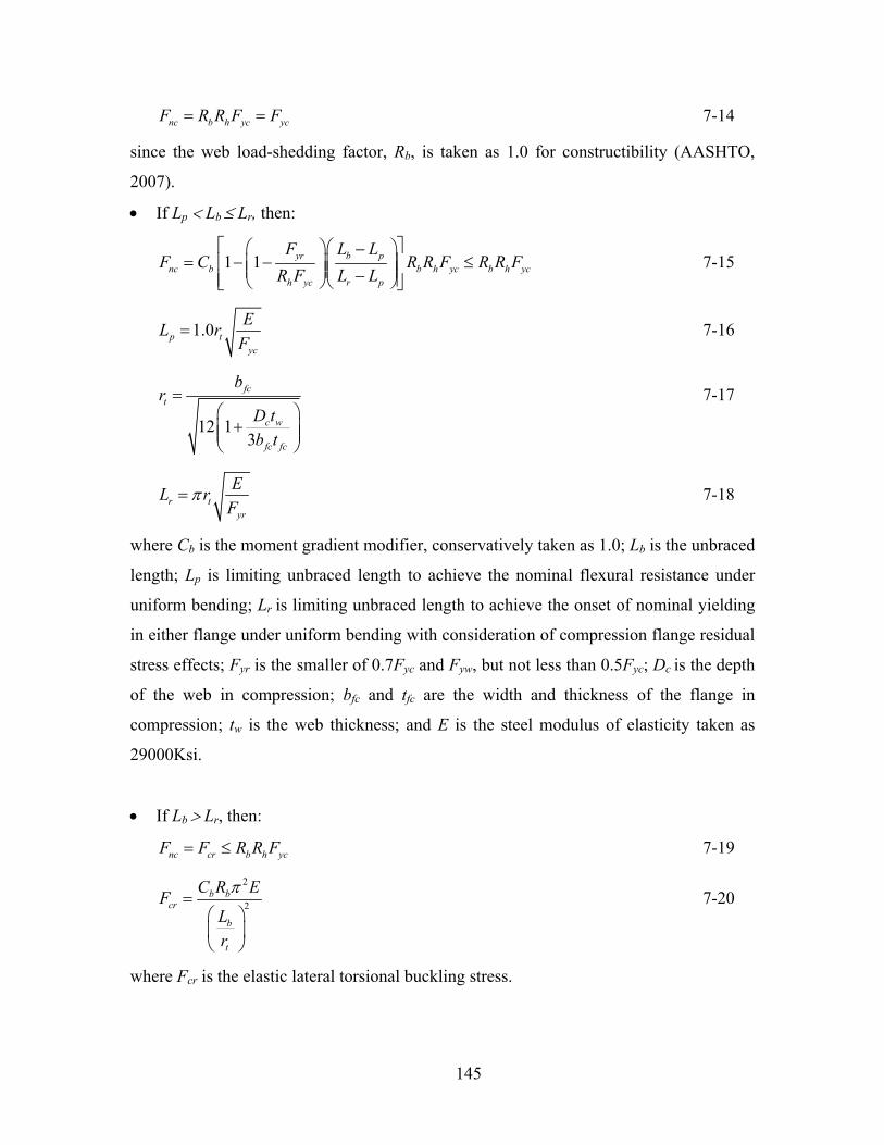
145
nc b h yc ycF R R F F= = 7-14
since the web load-shedding factor, Rb, is taken as 1.0 for constructibility (AASHTO,
2007).
• If Lp < Lb ≤ Lr, then:
1 1 yr b pnc b b h yc b h yc
h yc r p
F L LF C R R F R R F
R F L L
⎡ ⎤⎛ ⎞⎛ ⎞−= − − ≤⎢ ⎥⎜ ⎟⎜ ⎟⎜ ⎟⎜ ⎟−⎢ ⎥⎝ ⎠⎝ ⎠⎣ ⎦
7-15
1.0p tyc
EL rF
= 7-16
12 13
fct
c w
fc fc
br
D tb t
=⎛ ⎞
+⎜ ⎟⎜ ⎟⎝ ⎠
7-17
r tyr
EL rF
π= 7-18
where Cb is the moment gradient modifier, conservatively taken as 1.0; Lb is the unbraced
length; Lp is limiting unbraced length to achieve the nominal flexural resistance under
uniform bending; Lr is limiting unbraced length to achieve the onset of nominal yielding
in either flange under uniform bending with consideration of compression flange residual
stress effects; Fyr is the smaller of 0.7Fyc and Fyw, but not less than 0.5Fyc; Dc is the depth
of the web in compression; bfc and tfc are the width and thickness of the flange in
compression; tw is the web thickness; and E is the steel modulus of elasticity taken as
29000Ksi.
• If Lb > Lr, then:
nc cr b h ycF F R R F= ≤ 7-19
2
2b b
cr
b
t
C R EFLr
π=
⎛ ⎞⎜ ⎟⎝ ⎠
7-20
where Fcr is the elastic lateral torsional buckling stress.

146
7.3.1.2 Flange Local Buckling Resistance:
The local buckling resistance of a compression flange is taken as:
• If λ f ≤ λ pf, then:
nc b h yc ycF R R F F= = 7-21
• Otherwise:
1 1 yr f pfnc b b h yc b h yc
h yc rf pf
FF C R R F R R F
R Fλ λλ λ
⎡ ⎤⎛ ⎞⎛ ⎞−= − − ≤⎢ ⎥⎜ ⎟⎜ ⎟⎜ ⎟⎜ ⎟−⎢ ⎥⎝ ⎠⎝ ⎠⎣ ⎦
7-22
2fc
ffc
bt
λ = 7-23
0.38pfyc
EF
λ = 7-24
0.56rfyr
EF
λ = 7-25
where λf is the slenderness ratio for the compression flange, λpf is the limiting
slenderness ratio for a compact flange, and λrf is the limiting slenderness ratio for a
noncompact flange.
7.3.2 Probabilistic characteristics
In reliability analysis, the resistance R is taken as the product of the nominal
resistance (Rn) used in design and three factors that account for the uncertainties due to
material properties, fabrication and analysis (Nowak & Collins, 2000):
nR R MFP= 7-26
where M is the ratio of the actual to nominal material properties, F corresponds to the
ratio of the actual to nominal cross-sectional properties and P is the professional factor
defined as the ratio of the test to predicted capacity. The mean value of the resistance
model presented in Equation 7-24 and its corresponding λR and VR are defined as:
nR R M F P= 7-27

147
2 2 2
R
R M F P
M F P
V V V V
λ =
= + + 7-28
In this study, the resistance is taken as a lognormal variable. Table 7-4 contains
the probabilistic characteristics of the resistance parameters (Nowak et. al. 2006;
Galambos, 2004; White et. al. 2008):
Table 7-4. Probabilistic characteristics of resistance variables Variable λ V
Material (M) 1.06 0.06
Fabrication (F) 1.00 0.05
Professional factor (P) 1.10 0.05
Resistance (R) 1.166 0.093
7.4 Monte Carlo Simulation
In this work, the reliability analysis is applied to the factored loads and resistances
instead of the corresponding nominal values. This is because the load and resistance
factors have already been calibrated in the Specifications to meet a target reliability
index, βT=3.5. However, the reliability analysis is performed to study the effect of the
cross-frame spacing on the reliability of the flexural limit states for construction using a
Monte Carlo Simulation. This reliability evaluation is carried out for different Lb values.
As a result of this effort, fragility curves are developed in terms of the unbraced lengths
(Lb), which are useful to define maximum distance between the cross frames based on the
desired reliability level.
7.4.1 MCS for each cross-frame spacing
The following procedure is followed for each cross-frame distance to evaluate the
reliability of the limit state equations using the Monte Carlo Simulation:
1. Definition of the limit state equations in terms of the random variables:
The limit states described in Section 7.1 are restated in the Resistance – Demand
format to define zero ( 0LS = ) as the failure boundary for the reliability analysis, as
follows:

148
( )1 f yc bu lLS F f fφ= − + 7-29
213f nc bu lLS F f fφ ⎛ ⎞= − +⎜ ⎟
⎝ ⎠ 7-30
( )4 f yt bu lLS F f fφ= − + 7-31
6 0.6 yf lLS F f= − 7-32
2. Generate N specific random values for each random variable.
The Monte Carlo Simulation requires the generation of random numbers
according to the specific probabilistic distribution of the random variable considered.
Initially, the random numbers are generated distributed uniformly between 0 and
1. Common computer generators use a seed value to produce the required number of
random numbers, where a different seed value will produce a different set of random
numbers. Next, the normalized and uniform random numbers are transformed to random
numbers with the probabilistic characteristics given by the corresponding random
variable. This process is known as the Inverse Transformation Technique Method, where
the CDF of the random variable, Fx(xi), is equated to the generated uniformly random
number, ui, as indicated by Equation 7-30 and Figure 7-5:
( ) ( )1 X i i i X iF x u x F u−= ∴ = 7-33
Figure 7-5. Inverse Transformation Technique Method (Haldar & Mahadevan, 2000)

149
Therefore, to generate a set of standard normal random numbers, zi, the following
transformation is used:
( )1i iz u−= Φ 7-34
where Φ-1 is the inverse of the standard normal CDF. A standard normal distribution is
characterized by having a mean and a variance equal to 0 and 1, respectively. However,
a general normal random variable, xi, with mean and standard deviation (μx and σx)
different than 0 and 1, is related to zi as follows:
i x i xx zμ σ= + 7-35
Therefore, the normal random values for the load variables, fbu and fl, are
generated using Equation 7-32. For the resistance variables, Rn, a set of lognormal
random values are generated using the corresponding transformation, as follows:
( )ln lnexpi x i xx zμ σ= + 7-36
where ( ) 2ln ln
1ln2x x xμ μ σ= − and ( )2 2
ln ln 1x xVσ = + .
In this work, the random numbers of the variables are generated using the design
or factored value instead of the mean, since the load and resistance factors have already
been calibrated in the Specifications as mentioned previously.
A total of 1,000,000 random values were generated for each random variable (Rn,
fbu, fl), according to the probabilistic characteristics described previously. For example,
Figure 7-6 shows the generated values of fbu with μ=13.66Ksi and σ=1.68Ksi for the top
flange at the positive moment region of the end spans.

150
4 6 8 10 12 14 16 18 20 220
1
2
3
4
5
6
7
8x 10
4
fbu (Ksi)
Freq
uenc
y
Lm=150ft - TF - S1 - C2
Figure 7-6. Histogram of the simulated values of fbu with μ=13.66Ksi and σ=1.68Ksi
3. Evaluation of the limit state equations for the N realization sets and determination of
their probabilistic characteristics:
The limit state equations are evaluated for 1,000,000 (N) of realization sets of the
random variables defined in the previous step, as shown in Figure 7-7 for the ultimate
strength limit state of a compression flange. The means and the standard deviations of
these limit states were computed based on the evaluated N-set values using the
corresponding equations for discrete test data, as follows:
( )
1
22
1
1
1
n
ii
n
ii
x
x xn
x n xs
n
=
=
=
⎛ ⎞−⎜ ⎟
⎝ ⎠=−
∑
∑ 7-37
where x is the sample mean, sx is the sample standard deviation, n is the total number of
observations and xi is a single observation.

151
10 20 30 40 50 60 700
1
2
3
4
5
6
7
8x 10
4
LS2 (Ksi)
Freq
uenc
y
Lm=150ft - TF - S1 - C2
Figure 7-7. Histogram of the simulated limit state LS2 with μ=35.18Ksi and σ=4.88Ksi
4. Probability of failure:
The estimation of the probability of failure for a specific limit state equation
improves as N increases. If the evaluation of the limit state is less than zero, it means a
failure state. Therefore, an estimate of the probability of failure is defined as:
ff
NP
N= 7-38
where Nf is the number of simulation cycles that did not satisfy the limit state equation.
5. Evaluation of the accuracy and efficiency of the simulation:
The accuracy of the simulation is estimated assuming a theoretically correct
probability of failure close to zero (P= 10-4) corresponding to a reliability index (β) of
3.71, since a zero probability of failure cannot be achieved. Then, the error is computed
based on the 95% confidence interval of the estimated probability of failure (Haldar &
Mahadevan, 2000), as indicated by Equation 7-36.
1(%) 200% 20% P x
N Pε −
= = 7-39

152
Therefore, it can be affirmed that there is a 95% probability that the true
probability of failure will be in the range of 0.0001 ± 0.00002 (0.01% ± 0.002%) when
the simulation employs 1,000,000 realizations, for the assumed characteristics of the
random variables.
7.4.2 Fragility curves
Figure 7-8 shows an example of the CDFs generated for different Lb values of the
first two limit states for the top flange at the positive moment region of the end spans. It
is evident that the CDFs become more critical (i.e., moving toward zero) as Lb increases.
This effect is more pronounced in the ultimate strength limit state of the compression
flanges.
0 10 20 30 40 50 60 70 80 900
0.1
0.2
0.3
0.4
0.5
0.6
0.7
0.8
0.9
1
LS1 (Ksi)
F(x)
Lm=150ft - TF - S1 - C2
20 -10 0 10 20 30 40 50 60 70 80LS2 (Ksi)
Lm=150ft - TF - S1 - C2
Figure 7-8. Simulated CDFs of LS1 and LS2 for different Lb values in a straight bridge
The simulated probability of failure (Pf) and reliability indices (β) of each CDF
was plotted against the corresponding Lb to obtain the fragility curves for the limit states,
as shown in Figure 7-9. These curves represent a practical method to select the
maximum cross-frame spacing based on the maximum tolerated probability of failure or
reliability index.
Lb=15ft
Lb=100ft
Lb=15ft
Lb=100ft

153
10 20 30 40 50 60 70 80 90 1000
0.1
0.2
0.3
0.4
0.5
0.6
0.7
0.8
0.9
1S1 - TF - w
Lb (ft)
Pf
10 20 30 40 50 60 70 80 90 100-6
-4
-2
0
2
4
6S1 - TF - w
Lb (ft)
β
Figure 7-9. Fragility curves of LS2 using Monte Carlo Simulation
7.4.2.1 Straight Bridges
Figure 7-10, Figure 7-11 and Figure 7-12 show that the ultimate strength in the
compression flange is the governing limit state in the reliability analysis. It is also
observed that the reliability of the system is lower for short span bridges since the LFB
effects decrease as the length of the bridge increases. Table 7-5 shows the values of the
cross-frame spacing required to meet the code reliability index of 3.5.
Table 7-5. Maximum Lb (ft) corresponding to a code reliability level in straight bridges
End span
S1
Middle span
S3
Pier
S2
Lm=150ft 51 43 53
Lm =240ft 58 54 69
Lm =300ft 60 69 75

154
10 20 30 40 50 60 70 80 90 1000
0.1
0.2
0.3
0.4
0.5
0.6
0.7
0.8
0.9
1S1 - TF - P
Pf
Lm=150ft, LS1Lm=150ft, LS2Lm=150ft, LS6Lm=240ft, LS1Lm=240ft, LS2Lm=240ft, LS6Lm=300ft, LS1Lm=300ft, LS2Lm=300ft, LS6
10 20 30 40 50 60 70 80 90 100-0.5
0
0.5
1
1.5
2
2.5
3
3.5
4
4.5
5S1 - TF - P
β
Lm=150ft, LS1Lm=150ft, LS2Lm=150ft, LS6Lm=240ft, LS1Lm=240ft, LS2Lm=240ft, LS6Lm=300ft, LS1Lm=300ft, LS2Lm=300ft, LS6Code
10 20 30 40 50 60 70 80 90 1000
0.1
0.2
0.3
0.4
0.5
0.6
0.7
0.8
0.9
1S1 - TF - w
Lb (ft)
Pf
Lm=150ft, LS1Lm=150ft, LS2Lm=150ft, LS6Lm=240ft, LS1Lm=240ft, LS2Lm=240ft, LS6Lm=300ft, LS1Lm=300ft, LS2Lm=300ft, LS6
10 20 30 40 50 60 70 80 90 100-0.5
0
0.5
1
1.5
2
2.5
3
3.5
4
4.5
5S1 - TF - w
Lb (ft)
β
Lm=150ft, LS1Lm=150ft, LS2Lm=150ft, LS6Lm=240ft, LS1Lm=240ft, LS2Lm=240ft, LS6Lm=300ft, LS1Lm=300ft, LS2Lm=300ft, LS6Code
Figure 7-10. Fragility curves for the end-span sections in straight bridges with Lm=150ft
10 20 30 40 50 60 70 80 90 1000
0.1
0.2
0.3
0.4
0.5
0.6
0.7
0.8
0.9
1S3 - TF - P
Pf
Lm=150ft, LS1Lm=150ft, LS2Lm=150ft, LS6Lm=240ft, LS1Lm=240ft, LS2Lm=240ft, LS6Lm=300ft, LS1Lm=300ft, LS2Lm=300ft, LS6
10 20 30 40 50 60 70 80 90 100-0.5
0
0.5
1
1.5
2
2.5
3
3.5
4
4.5
5S3 - TF - P
β
Lm=150ft, LS1Lm=150ft, LS2Lm=150ft, LS6Lm=240ft, LS1Lm=240ft, LS2Lm=240ft, LS6Lm=300ft, LS1Lm=300ft, LS2Lm=300ft, LS6Code

155
10 20 30 40 50 60 70 80 90 1000
0.1
0.2
0.3
0.4
0.5
0.6
0.7
0.8
0.9
1S3 - TF - w
Pf
Lm=150ft, LS1Lm=150ft, LS2Lm=150ft, LS6Lm=240ft, LS1Lm=240ft, LS2Lm=240ft, LS6Lm=300ft, LS1Lm=300ft, LS2Lm=300ft, LS6
10 20 30 40 50 60 70 80 90 100-0.5
0
0.5
1
1.5
2
2.5
3
3.5
4
4.5
5S3 - TF - w
β
Lm=150ft, LS1Lm=150ft, LS2Lm=150ft, LS6Lm=240ft, LS1Lm=240ft, LS2Lm=240ft, LS6Lm=300ft, LS1Lm=300ft, LS2Lm=300ft, LS6Code
Figure 7-11. Fragility curves for the Lm sections in straight bridges with Lm =150ft
10 20 30 40 50 60 70 80 90 1000
0.1
0.2
0.3
0.4
0.5
0.6
0.7
0.8
0.9
1S2 - BF - w
Lb (ft)
Pf
Lm=150ft, LS1Lm=150ft, LS2Lm=150ft, LS6Lm=240ft, LS1Lm=240ft, LS2Lm=240ft, LS6Lm=300ft, LS1Lm=300ft, LS2Lm=300ft, LS6
10 20 30 40 50 60 70 80 90 100-0.5
0
0.5
1
1.5
2
2.5
3
3.5
4
4.5
5S2 - BF - w
Lb (ft)
β
Lm=150ft, LS1Lm=150ft, LS2Lm=150ft, LS6Lm=240ft, LS1Lm=240ft, LS2Lm=240ft, LS6Lm=300ft, LS1Lm=300ft, LS2Lm=300ft, LS6Code
Figure 7-12. Fragility curves for the pier sections in straight bridges with Lm =150ft
7.4.2.2 Skewed Bridges
From Figure 7-13, Figure 7-14, Figure 7-15 and Table 7-6, it is observed that the
skew angle does not affect the reliability of the bridges and the same results obtained for
straight bridges apply in this case. Appendix E contains the remaining figures
corresponding to θ=45° and 60°.
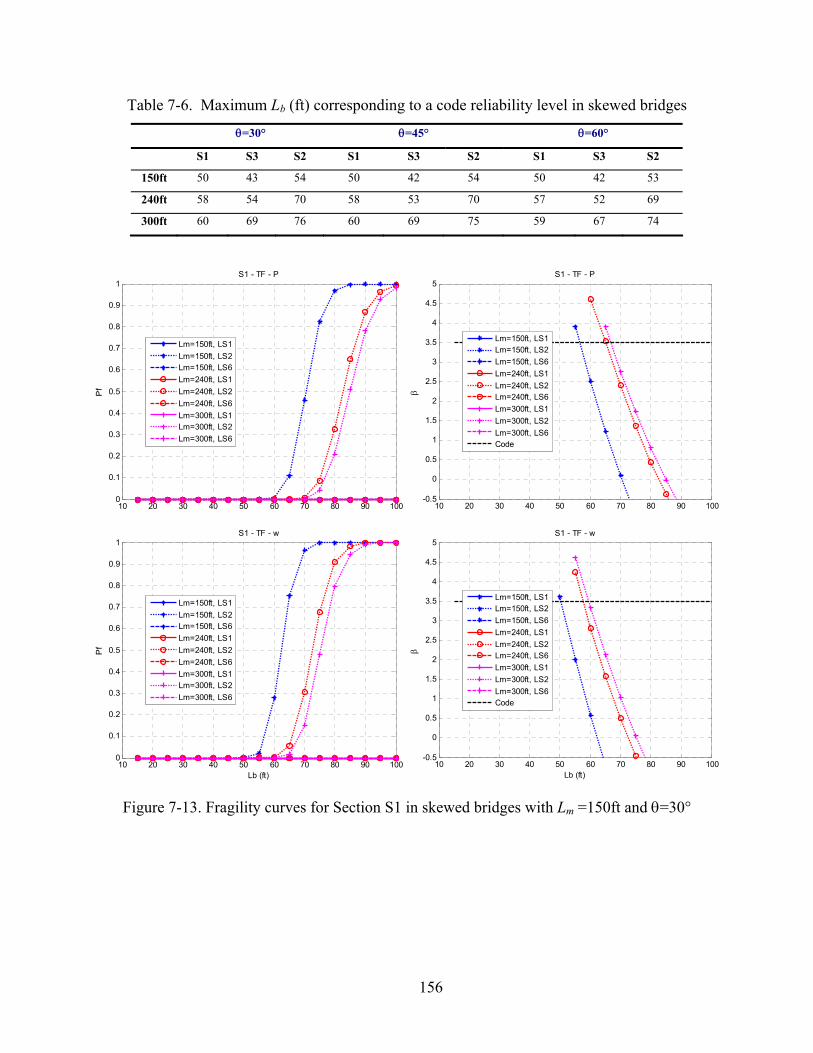
156
Table 7-6. Maximum Lb (ft) corresponding to a code reliability level in skewed bridges
θ=30° θ=45° θ=60°
S1 S3 S2 S1 S3 S2 S1 S3 S2
150ft 50 43 54 50 42 54 50 42 53
240ft 58 54 70 58 53 70 57 52 69
300ft 60 69 76 60 69 75 59 67 74
10 20 30 40 50 60 70 80 90 1000
0.1
0.2
0.3
0.4
0.5
0.6
0.7
0.8
0.9
1S1 - TF - P
Pf
Lm=150ft, LS1Lm=150ft, LS2Lm=150ft, LS6Lm=240ft, LS1Lm=240ft, LS2Lm=240ft, LS6Lm=300ft, LS1Lm=300ft, LS2Lm=300ft, LS6
10 20 30 40 50 60 70 80 90 100-0.5
0
0.5
1
1.5
2
2.5
3
3.5
4
4.5
5S1 - TF - P
β
Lm=150ft, LS1Lm=150ft, LS2Lm=150ft, LS6Lm=240ft, LS1Lm=240ft, LS2Lm=240ft, LS6Lm=300ft, LS1Lm=300ft, LS2Lm=300ft, LS6Code
10 20 30 40 50 60 70 80 90 1000
0.1
0.2
0.3
0.4
0.5
0.6
0.7
0.8
0.9
1S1 - TF - w
Lb (ft)
Pf
Lm=150ft, LS1Lm=150ft, LS2Lm=150ft, LS6Lm=240ft, LS1Lm=240ft, LS2Lm=240ft, LS6Lm=300ft, LS1Lm=300ft, LS2Lm=300ft, LS6
10 20 30 40 50 60 70 80 90 100-0.5
0
0.5
1
1.5
2
2.5
3
3.5
4
4.5
5S1 - TF - w
Lb (ft)
β
Lm=150ft, LS1Lm=150ft, LS2Lm=150ft, LS6Lm=240ft, LS1Lm=240ft, LS2Lm=240ft, LS6Lm=300ft, LS1Lm=300ft, LS2Lm=300ft, LS6Code
Figure 7-13. Fragility curves for Section S1 in skewed bridges with Lm =150ft and θ=30°

157
10 20 30 40 50 60 70 80 90 1000
0.1
0.2
0.3
0.4
0.5
0.6
0.7
0.8
0.9
1S3 - TF - P
Pf
Lm=150ft, LS1Lm=150ft, LS2Lm=150ft, LS6Lm=240ft, LS1Lm=240ft, LS2Lm=240ft, LS6Lm=300ft, LS1Lm=300ft, LS2Lm=300ft, LS6
10 20 30 40 50 60 70 80 90 100-0.5
0
0.5
1
1.5
2
2.5
3
3.5
4
4.5
5S3 - TF - P
β
Lm=150ft, LS1Lm=150ft, LS2Lm=150ft, LS6Lm=240ft, LS1Lm=240ft, LS2Lm=240ft, LS6Lm=300ft, LS1Lm=300ft, LS2Lm=300ft, LS6Code
10 20 30 40 50 60 70 80 90 1000
0.1
0.2
0.3
0.4
0.5
0.6
0.7
0.8
0.9
1S3 - TF - w
Lb (ft)
Pf
Lm=150ft, LS1Lm=150ft, LS2Lm=150ft, LS6Lm=240ft, LS1Lm=240ft, LS2Lm=240ft, LS6Lm=300ft, LS1Lm=300ft, LS2Lm=300ft, LS6
10 20 30 40 50 60 70 80 90 100-0.5
0
0.5
1
1.5
2
2.5
3
3.5
4
4.5
5S3 - TF - w
Lb (ft)
β
Lm=150ft, LS1Lm=150ft, LS2Lm=150ft, LS6Lm=240ft, LS1Lm=240ft, LS2Lm=240ft, LS6Lm=300ft, LS1Lm=300ft, LS2Lm=300ft, LS6Code
Figure 7-14. Fragility curves for Section S3 in skewed bridges with Lm =150ft and θ=30°
10 20 30 40 50 60 70 80 90 1000
0.1
0.2
0.3
0.4
0.5
0.6
0.7
0.8
0.9
1S2 - BF - w
Lb (ft)
Pf
Lm=150ft, LS1Lm=150ft, LS2Lm=150ft, LS6Lm=240ft, LS1Lm=240ft, LS2Lm=240ft, LS6Lm=300ft, LS1Lm=300ft, LS2Lm=300ft, LS6
10 20 30 40 50 60 70 80 90 100-0.5
0
0.5
1
1.5
2
2.5
3
3.5
4
4.5
5S2 - BF - w
Lb (ft)
β
Lm=150ft, LS1Lm=150ft, LS2Lm=150ft, LS6Lm=240ft, LS1Lm=240ft, LS2Lm=240ft, LS6Lm=300ft, LS1Lm=300ft, LS2Lm=300ft, LS6Code
Figure 7-15. Fragility curves for Section S2 in skewed bridges with Lm =150ft and θ=30°

158
7.4.2.3 Curved Bridges
Figure 7-16 - Figure 7-21, Table 7-7 and Table 7-8 show that the critical cross-
frame spacing is obtained at the end span of the exterior girder. The ultimate strength of
the compression flange is the limit state that governs in most cases. The reliability in the
exterior girder decreases for highly curved and long-span bridges. This is principally due
to the effect of fbu which is largely increased by the curvature and the span length.
The critical cross-frame distances in the middle span and the pier regions
corresponding to a code reliability level are not unfavorably affected by the span length
as shown in Table 7-7. However, these distances slightly decrease as the curvature is
higher.
In general, it is recommended to use temporary vertical supports at the end spans
during construction for highly curved and long bridges that do not meet the minimum
levels of tolerated reliability. Appendix F contains the additional fragility curves
corresponding to L/R=0.45 and 0.60.
Table 7-7. Maximum Lb (ft) corresponding to a code reliability level in G4 L/R=0.30 L/R=0.45 L/R=0.60
S1 S3 S2 S1 S3 S2 S1 S3 S2
150ft 37 40 46 25 37 42 <10 34 38
240ft 15 50 61 <10 48 57 <10 46 54
300ft <10 63 65 <10 62 62 <10 68 65
Table 7-8. Maximum Lb (ft) corresponding to a code reliability level in G1 L/R=0.30 L/R=0.45 L/R=0.60
S1 S3 S2 S1 S3 S2 S1 S3 S2
150ft 53 43 53 48 42 52 43 41 47
240ft 68 51 72 58 49 72 52 47 72
300ft 78 64 79 75 62 81 66 59 88

159
10 20 30 40 50 60 70 80 90 1000
0.1
0.2
0.3
0.4
0.5
0.6
0.7
0.8
0.9
1G4 - S1 - TF - P - L=150ft
Pf
L/R=0.30, LS1L/R=0.30, LS2L/R=0.30, LS6L/R=0.45, LS1L/R=0.45, LS2L/R=0.45, LS6L/R=0.60, LS1L/R=0.60, LS2L/R=0.60, LS6
10 20 30 40 50 60 70 80 90 100-0.5
0
0.5
1
1.5
2
2.5
3
3.5
4
4.5
5G4 - S1 - TF - P - L=150ft
β
L/R=0.30, LS1L/R=0.30, LS2L/R=0.30, LS6L/R=0.45, LS1L/R=0.45, LS2L/R=0.45, LS6L/R=0.60, LS1L/R=0.60, LS2L/R=0.60, LS6Code
10 20 30 40 50 60 70 80 90 1000
0.1
0.2
0.3
0.4
0.5
0.6
0.7
0.8
0.9
1G4 - S1 - BF - P - L=150ft
Pf
L/R=0.30, LS4L/R=0.30, LS6L/R=0.45, LS4L/R=0.45, LS6L/R=0.60, LS4L/R=0.60, LS6
10 20 30 40 50 60 70 80 90 100-0.5
0
0.5
1
1.5
2
2.5
3
3.5
4
4.5
5G4 - S1 - BF - P - L=150ft
β
L/R=0.30, LS4L/R=0.30, LS6L/R=0.45, LS4L/R=0.45, LS6L/R=0.60, LS4L/R=0.60, LS6Code
10 20 30 40 50 60 70 80 90 1000
0.1
0.2
0.3
0.4
0.5
0.6
0.7
0.8
0.9
1G4 - S1 - TF - w - L=150ft
Pf
L/R=0.30, LS1L/R=0.30, LS2L/R=0.30, LS6L/R=0.45, LS1L/R=0.45, LS2L/R=0.45, LS6L/R=0.60, LS1L/R=0.60, LS2L/R=0.60, LS6
10 20 30 40 50 60 70 80 90 100-0.5
0
0.5
1
1.5
2
2.5
3
3.5
4
4.5
5G4 - S1 - TF - w - L=150ft
β
L/R=0.30, LS1L/R=0.30, LS2L/R=0.30, LS6L/R=0.45, LS1L/R=0.45, LS2L/R=0.45, LS6L/R=0.60, LS1L/R=0.60, LS2L/R=0.60, LS6Code

160
10 20 30 40 50 60 70 80 90 1000
0.1
0.2
0.3
0.4
0.5
0.6
0.7
0.8
0.9
1G4 - S1 - BF - w - L=150ft
Lb (ft)
Pf
L/R=0.30, LS4L/R=0.30, LS6L/R=0.45, LS4L/R=0.45, LS6L/R=0.60, LS4L/R=0.60, LS6
10 20 30 40 50 60 70 80 90 100-0.5
0
0.5
1
1.5
2
2.5
3
3.5
4
4.5
5G4 - S1 - BF - w - L=150ft
Lb (ft)
β
L/R=0.30, LS4L/R=0.30, LS6L/R=0.45, LS4L/R=0.45, LS6L/R=0.60, LS4L/R=0.60, LS6Code
Figure 7-16. Fragility curves for section S1 in G4 with Lm =150ft -L/R=0.30
10 20 30 40 50 60 70 80 90 1000
0.1
0.2
0.3
0.4
0.5
0.6
0.7
0.8
0.9
1G4 - S3 - TF - P - L=150ft
Pf
L/R=0.30, LS1L/R=0.30, LS2L/R=0.30, LS6L/R=0.45, LS1L/R=0.45, LS2L/R=0.45, LS6L/R=0.60, LS1L/R=0.60, LS2L/R=0.60, LS6
10 20 30 40 50 60 70 80 90 100-0.5
0
0.5
1
1.5
2
2.5
3
3.5
4
4.5
5G4 - S3 - TF - P - L=150ft
β
L/R=0.30, LS1L/R=0.30, LS2L/R=0.30, LS6L/R=0.45, LS1L/R=0.45, LS2L/R=0.45, LS6L/R=0.60, LS1L/R=0.60, LS2L/R=0.60, LS6Code
10 20 30 40 50 60 70 80 90 1000
0.1
0.2
0.3
0.4
0.5
0.6
0.7
0.8
0.9
1G4 - S3 - BF - P - L=150ft
Pf
L/R=0.30, LS4L/R=0.30, LS6L/R=0.45, LS4L/R=0.45, LS6L/R=0.60, LS4L/R=0.60, LS6
10 20 30 40 50 60 70 80 90 100-0.5
0
0.5
1
1.5
2
2.5
3
3.5
4
4.5
5G4 - S3 - BF - P - L=150ft
β
L/R=0.30, LS4L/R=0.30, LS6L/R=0.45, LS4L/R=0.45, LS6L/R=0.60, LS4L/R=0.60, LS6Code

161
10 20 30 40 50 60 70 80 90 1000
0.1
0.2
0.3
0.4
0.5
0.6
0.7
0.8
0.9
1G4 - S3 - TF - w - L=150ft
Pf
L/R=0.30, LS1L/R=0.30, LS2L/R=0.30, LS6L/R=0.45, LS1L/R=0.45, LS2L/R=0.45, LS6L/R=0.60, LS1L/R=0.60, LS2L/R=0.60, LS6
10 20 30 40 50 60 70 80 90 100-0.5
0
0.5
1
1.5
2
2.5
3
3.5
4
4.5
5G4 - S3 - TF - w - L=150ft
β
L/R=0.30, LS1L/R=0.30, LS2L/R=0.30, LS6L/R=0.45, LS1L/R=0.45, LS2L/R=0.45, LS6L/R=0.60, LS1L/R=0.60, LS2L/R=0.60, LS6Code
10 20 30 40 50 60 70 80 90 1000
0.1
0.2
0.3
0.4
0.5
0.6
0.7
0.8
0.9
1G4 - S3 - BF - w - L=150ft
Lb (ft)
Pf
L/R=0.30, LS4L/R=0.30, LS6L/R=0.45, LS4L/R=0.45, LS6L/R=0.60, LS4L/R=0.60, LS6
10 20 30 40 50 60 70 80 90 100-0.5
0
0.5
1
1.5
2
2.5
3
3.5
4
4.5
5G4 - S3 - BF - w - L=150ft
Lb (ft)
β
L/R=0.30, LS4L/R=0.30, LS6L/R=0.45, LS4L/R=0.45, LS6L/R=0.60, LS4L/R=0.60, LS6Code
Figure 7-17. Fragility curves for Section S3 G4 with Lm =150ft -L/R=0.30
10 20 30 40 50 60 70 80 90 1000
0.1
0.2
0.3
0.4
0.5
0.6
0.7
0.8
0.9
1G4 - S2 - BF - w - L=150ft
Pf
L/R=0.30, LS1L/R=0.30, LS2L/R=0.30, LS6L/R=0.45, LS1L/R=0.45, LS2L/R=0.45, LS6L/R=0.60, LS1L/R=0.60, LS2L/R=0.60, LS6
10 20 30 40 50 60 70 80 90 100-0.5
0
0.5
1
1.5
2
2.5
3
3.5
4
4.5
5G4 - S2 - BF - w - L=150ft
β
L/R=0.30, LS1L/R=0.30, LS2L/R=0.30, LS6L/R=0.45, LS1L/R=0.45, LS2L/R=0.45, LS6L/R=0.60, LS1L/R=0.60, LS2L/R=0.60, LS6Code

162
10 20 30 40 50 60 70 80 90 1000
0.1
0.2
0.3
0.4
0.5
0.6
0.7
0.8
0.9
1G4 - S2 - TF - w - L=150ft
Lb (ft)
Pf
L/R=0.30, LS4L/R=0.30, LS6L/R=0.45, LS4L/R=0.45, LS6L/R=0.60, LS4L/R=0.60, LS6
10 20 30 40 50 60 70 80 90 100-0.5
0
0.5
1
1.5
2
2.5
3
3.5
4
4.5
5G4 - S2 - TF - w - L=150ft
Lb (ft)
β
L/R=0.30, LS4L/R=0.30, LS6L/R=0.45, LS4L/R=0.45, LS6L/R=0.60, LS4L/R=0.60, LS6Code
Figure 7-18. Fragility curves for Section S2 in G4 with Lm =150ft -L/R=0.30
10 20 30 40 50 60 70 80 90 1000
0.1
0.2
0.3
0.4
0.5
0.6
0.7
0.8
0.9
1G1 - S1 - TF - P - L=150ft
Pf
L/R=0.30, LS1L/R=0.30, LS2L/R=0.30, LS6L/R=0.45, LS1L/R=0.45, LS2L/R=0.45, LS6L/R=0.60, LS1L/R=0.60, LS2L/R=0.60, LS6
10 20 30 40 50 60 70 80 90 100-0.5
0
0.5
1
1.5
2
2.5
3
3.5
4
4.5
5G1 - S1 - TF - P - L=150ft
β
L/R=0.30, LS1L/R=0.30, LS2L/R=0.30, LS6L/R=0.45, LS1L/R=0.45, LS2L/R=0.45, LS6L/R=0.60, LS1L/R=0.60, LS2L/R=0.60, LS6Code
10 20 30 40 50 60 70 80 90 1000
0.1
0.2
0.3
0.4
0.5
0.6
0.7
0.8
0.9
1G1 - S1 - BF - P - L=150ft
Pf
L/R=0.30, LS4L/R=0.30, LS6L/R=0.45, LS4L/R=0.45, LS6L/R=0.60, LS4L/R=0.60, LS6
10 20 30 40 50 60 70 80 90 100-0.5
0
0.5
1
1.5
2
2.5
3
3.5
4
4.5
5G1 - S1 - BF - P - L=150ft
β
L/R=0.30, LS4L/R=0.30, LS6L/R=0.45, LS4L/R=0.45, LS6L/R=0.60, LS4L/R=0.60, LS6Code

163
10 20 30 40 50 60 70 80 90 1000
0.1
0.2
0.3
0.4
0.5
0.6
0.7
0.8
0.9
1G1 - S1 - TF - w - L=150ft
Pf
L/R=0.30, LS1L/R=0.30, LS2L/R=0.30, LS6L/R=0.45, LS1L/R=0.45, LS2L/R=0.45, LS6L/R=0.60, LS1L/R=0.60, LS2L/R=0.60, LS6
10 20 30 40 50 60 70 80 90 100-0.5
0
0.5
1
1.5
2
2.5
3
3.5
4
4.5
5G1 - S1 - TF - w - L=150ft
β
L/R=0.30, LS1L/R=0.30, LS2L/R=0.30, LS6L/R=0.45, LS1L/R=0.45, LS2L/R=0.45, LS6L/R=0.60, LS1L/R=0.60, LS2L/R=0.60, LS6Code
10 20 30 40 50 60 70 80 90 1000
0.1
0.2
0.3
0.4
0.5
0.6
0.7
0.8
0.9
1G1 - S1 - BF - w - L=150ft
Lb (ft)
Pf
L/R=0.30, LS4L/R=0.30, LS6L/R=0.45, LS4L/R=0.45, LS6L/R=0.60, LS4L/R=0.60, LS6
10 20 30 40 50 60 70 80 90 100-0.5
0
0.5
1
1.5
2
2.5
3
3.5
4
4.5
5G1 - S1 - BF - w - L=150ft
Lb (ft)
β
L/R=0.30, LS4L/R=0.30, LS6L/R=0.45, LS4L/R=0.45, LS6L/R=0.60, LS4L/R=0.60, LS6Code
Figure 7-19. Fragility curves for Section S1 in G1 with Lm =150ft -L/R=0.30
10 20 30 40 50 60 70 80 90 1000
0.1
0.2
0.3
0.4
0.5
0.6
0.7
0.8
0.9
1G1 - S3 - TF - P - L=150ft
Pf
L/R=0.30, LS1L/R=0.30, LS2L/R=0.30, LS6L/R=0.45, LS1L/R=0.45, LS2L/R=0.45, LS6L/R=0.60, LS1L/R=0.60, LS2L/R=0.60, LS6
10 20 30 40 50 60 70 80 90 100-0.5
0
0.5
1
1.5
2
2.5
3
3.5
4
4.5
5G1 - S3 - TF - P - L=150ft
β
L/R=0.30, LS1L/R=0.30, LS2L/R=0.30, LS6L/R=0.45, LS1L/R=0.45, LS2L/R=0.45, LS6L/R=0.60, LS1L/R=0.60, LS2L/R=0.60, LS6Code

164
10 20 30 40 50 60 70 80 90 1000
0.1
0.2
0.3
0.4
0.5
0.6
0.7
0.8
0.9
1G1 - S3 - BF - P - L=150ft
Pf
L/R=0.30, LS4L/R=0.30, LS6L/R=0.45, LS4L/R=0.45, LS6L/R=0.60, LS4L/R=0.60, LS6
10 20 30 40 50 60 70 80 90 100-0.5
0
0.5
1
1.5
2
2.5
3
3.5
4
4.5
5G1 - S3 - BF - P - L=150ft
β
L/R=0.30, LS4L/R=0.30, LS6L/R=0.45, LS4L/R=0.45, LS6L/R=0.60, LS4L/R=0.60, LS6Code
10 20 30 40 50 60 70 80 90 1000
0.1
0.2
0.3
0.4
0.5
0.6
0.7
0.8
0.9
1G1 - S3 - TF - w - L=150ft
Pf
L/R=0.30, LS1L/R=0.30, LS2L/R=0.30, LS6L/R=0.45, LS1L/R=0.45, LS2L/R=0.45, LS6L/R=0.60, LS1L/R=0.60, LS2L/R=0.60, LS6
10 20 30 40 50 60 70 80 90 100-0.5
0
0.5
1
1.5
2
2.5
3
3.5
4
4.5
5G1 - S3 - TF - w - L=150ft
β
L/R=0.30, LS1L/R=0.30, LS2L/R=0.30, LS6L/R=0.45, LS1L/R=0.45, LS2L/R=0.45, LS6L/R=0.60, LS1L/R=0.60, LS2L/R=0.60, LS6Code
10 20 30 40 50 60 70 80 90 1000
0.1
0.2
0.3
0.4
0.5
0.6
0.7
0.8
0.9
1G1 - S3 - BF - w - L=150ft
Lb (ft)
Pf
L/R=0.30, LS4L/R=0.30, LS6L/R=0.45, LS4L/R=0.45, LS6L/R=0.60, LS4L/R=0.60, LS6
10 20 30 40 50 60 70 80 90 100-0.5
0
0.5
1
1.5
2
2.5
3
3.5
4
4.5
5G1 - S3 - BF - w - L=150ft
Lb (ft)
β
L/R=0.30, LS4L/R=0.30, LS6L/R=0.45, LS4L/R=0.45, LS6L/R=0.60, LS4L/R=0.60, LS6Code
Figure 7-20. Fragility curves for Section S3 in G1 with Lm =150ft -L/R=0.30

165
10 20 30 40 50 60 70 80 90 1000
0.1
0.2
0.3
0.4
0.5
0.6
0.7
0.8
0.9
1G1 - S2 - BF - w - L=150ft
Pf
L/R=0.30, LS1L/R=0.30, LS2L/R=0.30, LS6L/R=0.45, LS1L/R=0.45, LS2L/R=0.45, LS6L/R=0.60, LS1L/R=0.60, LS2L/R=0.60, LS6
10 20 30 40 50 60 70 80 90 100-0.5
0
0.5
1
1.5
2
2.5
3
3.5
4
4.5
5G1 - S2 - BF - w - L=150ft
β
L/R=0.30, LS1L/R=0.30, LS2L/R=0.30, LS6L/R=0.45, LS1L/R=0.45, LS2L/R=0.45, LS6L/R=0.60, LS1L/R=0.60, LS2L/R=0.60, LS6Code
10 20 30 40 50 60 70 80 90 1000
0.1
0.2
0.3
0.4
0.5
0.6
0.7
0.8
0.9
1G1 - S2 - TF - w - L=150ft
Pf
L/R=0.30, LS4L/R=0.30, LS6L/R=0.45, LS4L/R=0.45, LS6L/R=0.60, LS4L/R=0.60, LS6
10 20 30 40 50 60 70 80 90 100-0.5
0
0.5
1
1.5
2
2.5
3
3.5
4
4.5
5G1 - S2 - TF - w - L=150ft
Lb (ft)
β
L/R=0.30, LS4L/R=0.30, LS6L/R=0.45, LS4L/R=0.45, LS6L/R=0.60, LS4L/R=0.60, LS6Code
Figure 7-21. Fragility curves for Section S2 in G1 with Lm =150ft -L/R=0.30
7.5 Concluding remarks
A reliability analysis was performed to develop fragility curves that allow the
designer to select the cross-frame spacing for deck placement conditions considering the
flexural limit states for constructibility that are directly affected by the cross-frame
spacing. The adopted structural loading and resistance models were described along with
their corresponding probabilistic characteristics. A Monte Carlo Simulation was
conducted for straight, skewed and curved steel I-girder bridges to obtain the fragility
curves that allow identifying the maximum cross-frame according to the maximum
tolerated level of risk. The following observations were established from this effort.

166
For all bridge types, the ultimate strength in the compression flange is the
governing limit state in the reliability analysis. Therefore, the fragility curves obtained in
this work may be valid for service conditions since the compression flange in these cases
act as a composite section.
For straight and skewed bridges, it was observed that the reliability of the system
is lower for short span bridges since the LFB effects decrease as the length of the bridge
increases. The results showed that the skew angle does not affect the reliability of the
skewed bridges and the same results obtained for straight bridges apply in this case.
For curved bridges, it was observed that the critical cross-frame spacing is
obtained at the end span of the exterior girder. The reliability in the exterior girder
decreases for highly curved and long-span bridges due to the effect of fbu, which is deeply
increased by the curvature and the span length. The critical cross-frame distances in the
middle span and the pier regions corresponding to a code reliability level are not
unfavorably affected by the span length. However, these distances slightly decrease as
the curvature is higher.
In general, it is recommended to use temporary vertical supports at the end spans
during construction for highly curved and long bridges that do not meet the minimum
levels of tolerated reliability.

167
Chapter 8: Summary, conclusions and recommendations
8.1 Summary
This work has resulted in the development of approximated equations that predict
the LFB in steel I-girder bridges during concrete deck placement. The effects on the
flexural limit state equations for constructibility of variables such as skew, curvature,
cross-frame spacing, girder cross section and casting sequence were evaluated as well. In
addition, the maximum allowed skews and curvatures were computed for straight bridges
based on the limit states for constructibility and the proposed LFB equations. Finally,
fragility curves were developed for steel I-girder bridges during construction that allow
selecting the maximum cross-frame according to the maximum tolerated level of risk.
Introductory material was presented in Chapter 1 including general information of
the research topic, the need for this project, the main research objectives and the research
methods. Chapter 2 presented the literature review of topics related to this research
project such as LFB, overhang loads, curved and skewed steel I-girder bridges,
specifications and structural reliability.
Chapter 3 discussed the principal modeling procedures employed to conduct FEA
in this project. A description of the material models, the finite elements and analyses
required to model the bridge behavior during deck placement conditions is included. A
validation of the modeling procedures was also presented based on the results from
different experimental tests.
The parametric study used to investigate the effects of the deck-placement process
on the LFB of steel I-girder bridges was described in Chapter 4. The description covered
the parametric variables, the loads, the structural design and the analyses for each
parametric configuration that properly represent the deck casting sequence.
Chapter 5 presented the results from the parametric study that allow formulating
approximate equations to predict the LFB in straight, skewed and curved steel I-girder
bridges during deck placement. The major-axis bending stresses were also analyzed,
where the principal contribution was made for curved.

168
In Chapter 6, the AASHTO flexural limit states for constructibility were evaluated
using the results from the parametric study along with the equations proposed in Chapter
5 to estimate the LFB. Initially, the critical sections along the bridge were identified and
the effects of the cross-frame spacing and the deck-placement sequence in the governing
limit states were evaluated as well. Finally, the maximum allowable skews and
curvatures for deck placement conditions were computed for bridges designed originally
as straight.
Chapter 7 described the reliability analysis performed to develop the fragility
curves. A general description of a structural reliability study is given initially, followed
by the definition of the structural loading and resistance models employed in this work.
Then, the Monte Carlo Simulations were performed for straight, skewed and curved steel
I-girder bridges resulting in the fragility curves that allow identifying the maximum
cross-frame spacing for deck-placement conditions according to the maximum tolerated
level of risk.
8.2 Conclusions
The bending stresses obtained during deck placement conditions in three-span
straight, skewed and curved steel I-girder bridges were evaluated in Chapter 5 using the
results obtained from a FEA parametric study. A symmetric deck casting sequence was
considered where the positive moment regions are poured first. The LFB stresses caused
by different sources were estimated by the curves that have the best fit to the numerical
critical stresses. The following major conclusions were established from this evaluation.
• Straight structures:
The major-axis bending stresses exhibited by the exterior girders of straight
bridges are independent of the cross-frame spacing. Therefore, these stresses may be
obtained from the structural analysis of either a simplified model that does not consider
explicitly the cross frames or a more detailed model involving any cross-frame distance.
For the positive moment regions, the LFB due to distributed loads was
satisfactorily predicted by the equation proposed in this work over the entire range of
cross-frame distances, principally at the end spans. Although the LFB obtained in the

169
middle span is lower, the same equations were proposed to simplify the approximations.
Comparisons with the code estimations showed that the Specifications are highly
conservative in all cases, especially for large cross-frame distances.
For concentrated loads, a linear regression considering the most external points
from the critical curves was performed to adjust the numerical stresses. These external
points correspond to models where the concentrated loads are placed at the middle of a
cross-frame spacing which is the critical location. The proposed equation for the bottom
flange governs over the code equation for cross-frame distances larger than 26ft.
However, both the code and the proposed approximations coincide for the top flange.
The LFB effect on the negative moment regions was approximated considering
only the distributed loading case since the contribution from the concentrated loads is
negligible. The results showed that the proposed equation satisfactorily predicts the LFB
in both flanges.
• Skewed structures
The results showed that skewed bridges exhibit LFB even when torsional loads
are not applied. However, in the presence of torsional effects, the LFB effect is slightly
more pronounced when the cross frames are oriented parallel to the supports. Therefore,
a perpendicular orientation of the cross frames is recommended for general skewed
bridges to increase the lateral stiffness of the structure. This perpendicular configuration
was adopted in this work to evaluate the LFB effects.
The results indicated that the major-axis bending in skewed bridges is not only
independent of the cross-frame spacing but also of the skew angle. Therefore, these
stresses may be taken from structural analyses performed for skewed bridges with any
cross-frame spacing and skew angle, including their simplified straight counterpart.
The LFB in the positive moment regions was approximated using curve fitting
models similar to the ones used for straight bridges. For distributed loads, a lower limit
was introduced in the proposed equation for the bottom flange since this flange exhibits
LFB even for closely spaced cross frames. The minimum LFB stress considered in the
bottom flange is proportional to the skew angle. The results were compared to the code
equation for overhang loads and significant overestimations of the LFB principally for
long cross-frame distances were found. For concentrated loads, the results showed that

170
the code equation for overhang loads fails to satisfactorily predict the LFB in most of the
cases, principally in the bottom flange.
The LFB in the negative moment regions was approximated in this work by a
constant term that depends on the skew angle. This approximation was adopted to
conservatively estimate the stresses which do not exhibit a consistent trend in these
regions. The results also indicated that the code recommendation of using 10Ksi for the
unfactored LFB stresses in skewed bridges is conservative even compared to factored
stresses.
• Curved structures
The evaluation of the bending stresses in curved bridges indicated that the major-
axis bending and the LFB are deeply affected by the curvature and the position of the
girder, i.e. outer or inner girder.
The analyses showed that the major-bending stresses in curved bridges are
independent of the cross-frame spacing. However, they increase linearly with the
curvature at the positive moment regions of the end spans. Conversely, these stresses at
the middle span of the outer girder are not significantly affected by the curvature. A
linear model was proposed to estimate the major-bending effects in the positive moment
regions of both exterior girders. This model computes the major-axis bending in curved
bridges based on the major-axis bending stresses exhibited by their straight counterpart.
Therefore, the proposed equation allows estimating the major-axis bending in curved
bridges from structural analyses of simplified straight bridges. In the negative moment
regions, the major-bending stresses also exhibit a linear trend but it is independent of the
span length.
The assumption of computing the major-axis bending based on a simplified
straight model with the real arc length of the curved girder does not help to represent the
curvature effects on these stresses. In fact, the AASHTO recommendation of ignoring
the curvature effects for fbu when L/R is lower than 0.06 introduces an error of
approximately 10% in long span bridges.
The LFB in curved girders is caused by both the curvature and the overhang
loads. However, it was shown that the participation of the overhang loads in the LFB is
low compared to the curvature effects. In fact, the overhang-to-curvature effect ratio

171
reduces as the length of the span and the curvature increase. Therefore, the overhang
term was dropped from the final expression proposed for the LFB which simplifies to the
curvature term only. However, the torsional effects due to overhang loads are implicitly
considered since the curve fitting process is applied to the total LFB obtained from the
parametric study. A comprehensive formulation to estimate the LFB effects due to
curvature was developed for distributed and concentrated loads, respectively. The critical
case between the top and bottom flanges was selected to define the equations proposed in
this work to estimate the LFB in curved bridges.
The results indicated that the LFB is practically unaffected by the variation of the
curvature, a slight effect was only observed in the positive moment regions of the middle
span. This observation indicates that these effects need to be considered even in bridges
with large curvature radii.
The equations proposed in this project to estimate the LFB in curved bridges work
adequately in both exterior girders. Significant reductions were found in most of the
cases compared to the estimations given by the AASHTO.
The major-axis bending effects in the AASHTO equation were computed using
both the numerical and the estimated major-axis bending stresses, obtaining similar
results. The estimated major-axis bending stresses correspond to the stresses computed
using the equation proposed in this work to estimate fbu in curved bridges from the results
obtained in their straight counterpart. Therefore, the LFB in a curved bridge can be
conservatively approximated using the code equation together with the major-axis
bending from a corresponding straight bridge. The advantage of the proposed equations
over the code approximation is that it is not required to know in advance the major-
bending effects to compute the LFB. However, the principal disadvantage is that
different expressions are required to define the effects of distributed and concentrated
loads, while the code approximation consists of one single equation that applies for all
load cases independent of the girder location and flange position.
However, the results from the parametric study indicated that the code equation
fails to predict the LFB due to distributed loads at the inner girder of highly curved
bridges with long spans. Therefore, it is recommended to use the equation proposed in
this work which predicts satisfactorily the LFB in all cases. It was also observed that the

172
bottom flange under concentrated loads exhibits the most critical LFB effects compared
to the top flange, especially for short span lengths.
The results indicated that the outer girder exhibits the most critical combined
bending effects. On the contrary, the curvature decreases the magnitude of the major-
bending stresses in the inner girder resulting in a combined bending action much lower
than that corresponding to the outer girder. Therefore, the design of both exterior girders
shall be based on the evaluation of the outer girder, unless an optimization of the inner
girder is pursued. In that case, the effects of the girder stiffness in the behavior of the
whole cross section of the deck shall be investigated.
The first part of Chapter 6 was intended to evaluate the behavior of the limit states
for constructibility based on the FEA results obtained from the parametric study. The
following major results were obtained.
For the skewed bridges analyzed in this work, it was observed that the effect on
the limit states of the girder position, the cross-frame orientation and the skew angle is
almost negligible. However, the cross-frame spacing has a significant effect on the limit
state of discretely braced flanges in compression principally in the positive moment
regions, since the LFB depends on the cross-frame distance and the capacity of the flange
reduces as this parameter increases.
It was also observed that the cross sections of the end and middle spans are
controlled by the casts where the concrete is placed over the complete positive moment
region. The compression flanges in both spans are governed by the ultimate strength
limit state. The negative moment regions are controlled by the last casting stage. The
flanges in compression are governed by the yielding limit state for short span length
bridges. However, the web bend-buckling limit state governs the compression flanges for
longer spans.
In curved bridges, the results showed that both the curvature and the cross-frame
spacing highly affect the limit state ratios in the positive moment regions of the outer
girder. However, a stress relief was observed in the inner girder caused by the length
adjustments due to curvature. Additionally, the LFB exhibited by the inner girder is
relieved since its eccentricity with respect to the supports is smaller. In fact, the LFB

173
undergoes a reversing effect in the inner girder compared to its straight counterpart. This
is caused from the torsional effects that are controlled by the curvature being
counteracted by the overhang load effects in the inner girder.
It was observed that the variables that most affect the limit states are the curvature
followed by the cross-frame spacing. The sections of the end and middle spans are
controlled by the casts that consider the concrete over the total positive moment regions.
The ultimate strength is the limit state that principally governs the compression flanges in
these sections. However, the yielding limit state may control in short span lengths with
high curvatures.
As for skewed bridges, the negative moment regions are controlled by the last
casting stage. The yielding limit state governs the compression flanges of bridges with
short spans and the web bend-buckling limit state becomes significant in the pier regions
for long span bridges.
None of the critical limit state values resulted from a casting stage where the
finishing machine is considered.
In the second part of Chapter 6, the maximum allowed skews and curvatures were
computed for straight bridges based on the limit states for constructibility and the LFB
equations proposed in Chapter 5. For skewed bridges, it was observed that the
maximum cross-frame spacing in skewed bridges is controlled by the ultimate strength
limit state in the compression flange. Conversely, the tension flange seems to be
unaffected by the skew angle.
On the other hand, the maximum allowed curvature is controlled in most of the
cases by the end-span cross section in the outer girder. It was also shown that the
ultimate strength limit state of the compression flange controls the maximum allowable
curvature for large cross-frame distances. Comparisons with the code recommendation
about the maximum cross-frame spacing in curved bridges showed that this specification
is adequate in short span bridges when the distance between cross frames is less than
approximately 40ft. However, long span bridges present an allowable curvature lower
than the one recommended in the code when the cross sections are designed from a
straight girder formulation.

174
A reliability analysis employing a Monte Carlo Simulation was performed in
Chapter 7 to develop fragility curves that allow the designer to select the cross-frame
spacing for deck placement conditions. The following observations were established
from this effort.
For all bridge types, the ultimate strength in the compression flange is the
governing limit state in the reliability analysis. Therefore, the fragility curves obtained
may be valid for service conditions since the compression flange in these cases acts as a
composite section.
For straight and skewed bridges, it was observed that the reliability of the system
is lower for short span bridges, since the LFB effects decrease as the length of the bridge
increases. The results showed that the skew angle does not affect the reliability of the
skewed bridges and the same results obtained for straight bridges apply in this case.
For curved bridges, it was observed that the critical cross-frame spacing is
obtained at the end span of the exterior girder. The reliability in the exterior girder
decreases for highly curved and long-span bridges due to the effect of fbu, which is deeply
increased by the curvature and the span length. The critical cross-frame distances in the
middle span and the pier regions corresponding to a code reliability level are not
unfavorably affected by the span length. However, these distances slightly decrease as
the curvature is higher.
In general, it is recommended to use temporary vertical supports at the end spans
during construction for highly curved and long bridges that do not meet the minimum
levels of tolerated reliability.
8.3 Recommendations
The results presented in this work correspond to steel I-girder bridges with the
specific characteristics described in the parametric study. Additional parametric
variables such as overhang length, girder spacing, number of girders, number of spans,
yielding strength, etc., should be incorporated in future research efforts to complement
the existing conclusions. In particular, the parametric study is based on the loads factored
according to the Strength I load combination of the Specifications. Additional load

175
combinations may be considered where the LFB effects due to wind are analyzed. In
addition, in this study, a symmetric deck casting sequence was considered. The
evaluation of critical conditions exhibited during unsymmetrical sequences would be a
beneficial supplement to the existing work.
The present work is focused on the evaluation of the flexural bending stresses
exhibited by the girder flanges. Future work incorporating shear stresses, deflections and
distortions will provide the engineer with the criteria required to evaluate the complete
structural behavior of steel I-girder bridges during construction. Moreover, the
evaluation of the internal forces in the members of the lateral bracing system will
contribute to improve the corresponding design specifications.
It is suggested that some of the results obtained in this work be validated by
conducting experimental tests.

176
References
AASHTO. (1992). Standard Specifications for Highway Bridges (15th ed.). Washington, DC: Author.
AASHTO. (1994). LRFD Bridge Design Specifications, S.I. units. Washington, DC:
Author. AASHTO. (1998). LRFD Bridge Design Specifications, Customary U.S. units (2nd ed.).
Washington, DC: Author. AASHTO. (2003). Guide Specifications for Horizontally Curved Steel Girder Highway
Bridges. Washington, DC: Author. AASHTO. (2004). LRFD Bridge Design Specifications, Customary U.S. units (3rd ed.).
Washington, DC: Author. AASHTO. (2007). LRFD Bridge Design Specifications, Customary U.S. units (4th ed.) –
2008 Interim Revisions. Washington, DC: Author. Abaqus. (2002). Version 6.3 Documentation. Pawtucket, RI: Hibbit, Karlsson &
Sorensen. American Concrete Institute. (2002). Building code requirements for structural concrete
and commentary, ACI 318-02. Farmington Hills, MI: Author. Applied Technology Council. (1996). Seismic evaluation and retrofit of concrete
buildings. Redwood City, CA: Author. Barker, M., & Zacher, J. (1997). Reliability of Inelastic Load Capacity Rating limits for
Steel bridges. Journal of Bridge Engineering, 2(2), 45-52. Barth, K., & Wu, H. (2006). Efficient Nonlinear Finite Element Modeling of Slab on
Steel Stringer Bridges. Finite Elements in Analysis and Design, 42(14), 1304-1313.
Beal, D. (1978). Horizontally Curved Bridges: New York field testing and design studies
(Vol. 61). Albany, NY: New York State Department of Transportation. Beal, D., & Kissane, R. (1971). Field Testing of Horizontally Curved Steel Girder
Bridges. Albany, NY: New York State Department of Transportation. Beckmann, F., & Medlock, R. (2005). Skewed Bridges and Girders Movements due to
rotations and differential deflections. Paper presented at 2005 World Steel Bridge – Symposium and Workshops. Orlando, FL: National Steel Bridge Alliance.
177
Bell, B., & Linzell, D. (2007). Erection Procedure Effects on Deformations and stresses
in a Large-radius, horizontally curved, I-girder Bridge. Journal of Bridge Engineering, 12(4), 467-476.
Brokenbrough, R. (1986). Distribution factors for curved I-girder bridges. Journal of
Structural Engineering, 112(10), 2200-2215. Chang, C., White, D., Beshah, F., & Wright, W. (2005). Design Analysis of Curved I-
Girder Bridge Systems – An Assessment of Modeling Strategies. Paper presented at the Annual Stability Conference. Montreal & Quebec: Structural Stability Research Council.
Chavel, B. W., & Earls, C. J. (2006a). Construction of a Horizontally Curved Steel I-
Girder Bridge, Part I: Erection Sequence. Journal of Bridge Engineering, 11(1), 81-90.
Chavel, B. W., & Earls, C. J. (2006b). Construction of a Horizontally Curved Steel I-
Girder Bridge, Part II: Inconsistent Detailing. Journal of Bridge Engineering, 11(1), 91-98.
Cheng, G., Xu, L., & Jiang, L. (2006). A sequential approximate programming strategy
for reliability-based structural optimization. Computers & Structures, 84(21), 1353-1367.
Choo, T., Linzell, D., Lee, J., & Swanson, J. (2005). Response of a continuous, skewed,
steel bridge during deck placement. Journal of Constructional Steel Research, 61(5), 567-586.
Coletti, D., & Yadlosky, J. (2005). Behavior and analysis of curved and skewed steel
girder bridges. Paper presented at 2005 World Steel Bridge – Symposium and Workshops. Orlando, FL: National Steel Bridge Alliance.
Czarnecki, A., & Nowak, A. (2006). System Reliability Assessment of Steel Girder
Bridges. In M. Pandey, W. Xie and L. Xu (Eds.), Advances in Engineering Structures, Mechanics and Construction, (pp. 699-710). Canada: Springer Netherlands.
Davidson, J., & Madhavan, M. (2006). Definition of flange compactness for I-beams that
are subjected to combined primary bending and torsion or lateral flexure. Paper presented at the 17th Analysis and Computation Specialty Conference. St. Louis, MO: Structural Engineering and Public Safety.
Davidson, J., & Yoo, C. (2000). Evaluation of Strength Formulations for Horizontally
Curved Flexural Members. Journal of Bridge Engineering, 5(3), 200-207.

178
Davidson, J., & Yoo, C. (1996). Local buckling of curved I-girder flanges. Journal of Structural Engineering, 122(8), 936-947.
Davidson, J., Keller, M., & Yoo, C. (1996). Cross-frame spacing and parametric effects
in horizontally curved I-girder bridges. Journal of Structural Engineering, 122(9), 1089-1096.
Davidson, J., & Yoo, C. (2003). Effects of distortion on strength of curved I-shaped
bridge girders. Transportation Research Record, 1845, 48-56. Davidson, J., Abdalla, R., & Madhavan, M. (2002). Design and construction of modern
curved bridges, Report No. 01223. Huntsville, AL: University Transportation Center for Alabama.
Davidson, J., Ballance, S. & Yoo, C. (1999). Analytical model of curved I-girder web
panels subjected to bending. Journal of Bridge Engineering, 4(3), 204-212. Davidson, J., Ballance, S. & Yoo, C. (1999). Finite displacement behavior of curved I-
girder webs subjected to bending. Journal of Bridge Engineering, 4(3), 213 -220. Davidson, J., Ballance, S., & Yoo, C. (1999). Effects of longitudinal stiffeners on curved
I-girder webs. Journal of Bridge Engineering, 5(2), 171 -178. Davidson, J., Keller, M. & Yoo, C. (1996). Cross-frame spacing and parametric effects in
horizontally curved I-girder bridges. Journal of Structural Engineering, 122(9), 1089-1096.
De Polo, D. & Linzell, D. (2005). Evaluation of live load lateral flange bending
distribution for a horizontally curved I-girder bridge. Paper presented at the Transportation Research Board 84th Annual Meeting. Washington, DC: TRB.
Domalik, D., Shura, J., & Linzell, D. (2005). Design and Field Monitoring of
Horizontally Curved Steel Plate Girder Bridge. Transportation Research Board, 1928, 83–91.
Duwadi, S., Grubb, M., Yoo, C., & Hartmann, J. (2000). Federal Highway
Administration’s Horizontally Curved Steel Bridge Research Project – An update.Transportation Research Record, 1696, 152-161.
Eamon, C., Nowak, A., Ritter, M., & Murphy, J. (2000). Reliability-based criteria for
load and resistance factor design code for wood bridges. Transportation Research Record, 1696, 316-322.
Ellingwood, B. (1985). Probability-based load criteria for structural design. Paper
published in A Chronicle of Selected of NIST publications 1901-2000. Washington, DC: National Institute of Standards and Technology.

179
Ellingwood, B., Galambos, T., MacGregor, J., and Cornell, C. (1980). Development of a
Probability Based Load Criteria for American National Standard A58. Washington, D.C.: National Bureau of Standards.
FEMA. (2000a). FEMA 356 – Pre-standard and commentary for the seismic
rehabilitation of building. Washington D.C.: Author. FEMA. (2000b). FEMA 350 – Recommended Seismic Design Criteria for New Steel
Moment-Frame Buildings. Washington D.C.: SAC Joint Venture. FEMA. (2003). NEHRP – Recommended provisions for seismic regulation for new
buildings and other structures, Part I: Provisions, Part 2: Commentary, FEMA450. Washington, D.C.: Building Seismic Safety Council.
Foschi, R., Li, H., & Zhang, J. (2002). Reliability and performance-based design: a
computational approach and applications. Structural Safety, 24(2-4), 205-218. Galambos, T. (2004). Reliability of the Member Stability Criteria in the 2005 AISC
Specification. Steel Structures, 4, 223-230. Galambos, T., Hajjar, J., Huang, W., Pulver, B., Leon, R. & Rudie, B. (2000).
Comparison of measured and computed stresses in a steel curved girder bridge. Journal of Bridge Engineering, 5(3), 191-199.
Galindez, N., & Barth, K. (2008). An assessment of the levels of lateral flange bending in
skewed and curved girder bridges due to concrete placement. Paper presented at the Annual Stability Conference. Nashville, TN: Structural Stability Research Council.
Gayton, N., Mohamed, G., Sorensen, J., Pendola, M., & Lemaire, M. (2004). Calibration
methods for reliability-based design codes. Structural Safety, 26(1), 91-121. Grubb, M. (1991). Design for Concrete Deck Overhang Loads. Paper presented at the
National Steel Construction Conference. Washington, DC: American Institute of Steel Construction.
Grubb, M., Yadlosky, J., & Duwadi, S. (1996). Construction issues in steel curved-girder
bridges. Transportation Research Record, 1544, 64-70. Hartmann, J. (2005). An experimental investigation of the flexural resistance of
horizontally curved steel I-girder systems. Ph.D. Dissertation, University of Maryland, College Park, MD.
Heins, C., & Jin, J. (1984). Live load distribution on braced curved I-girders. Journal of
Structural Engineering, 110(3), 523-530.

180
Herman, R., Helwig, T., Holt, J., Medlock, R., Romage, M., & Zhou, C. (2005). Lean-on
cross-frame bracing for steel girders with skewed supports. Paper presented at 2005 World Steel Bridge – Symposium and Workshops. Orlando, FL: National Steel Bridge Alliance.
Howell, T., & Earls, C. (2007). Curved Steel I-girder bridge response during construction
loading: effects of web plumbness. Journal of Bridge Engineering, 12(4), 485-493.
Huang, H., Shenton, H., & Chajes, M. (2004). Load distribution for a highly skewed
bridge: testing and analysis. Journal of Bridge Engineering, 9(6), 558-562. Issa, M., Yousif, A., & Issa, M. (2000). Effect of construction loads and vibrations on
new concrete bridge decks. Journal of Bridge Engineering, 5(3), 249-258. Jung, S. (2006). Inelastic strength behavior of horizontally curved composite I-girder
bridge structural systems. Ph.D. Dissertation, Georgia Institute of Technology,Atlanta, GA.
Jung, S., White, D., Beshah, F., & Wright, W. (2005). Ultimate Strength of Horizontally
– Curved Composite I-Girder Bridge Structural Systems. Paper presented at the Annual Stability Conference. Montreal & Quebec: Structural Stability ResearchCouncil.
Kansas Department of Transportation. (2005). Design Manual – Ch.5 Falsework design,
analysis and inspection. Kansas: Author. Khaloo, A., & Mirzabozorg, H. (2003). Load distribution factors in simply supported
skew bridges. Journal of Bridge Engineering, 8(4), 241-244. Kissane, R. (1978). Estimating Lateral Flange Bending in Curved Plate Girders. (Vol.
60). Albany, NY: New York State Department of Transportation. Kissane, R., & Beal, D. (1972). Field Testing of Horizontally Curved Steel Girder
Bridges (Vol. 8). Albany, NY: New York State Department of Transportation. Lee, J. & Fenves, G. (1998). Plastic-damage model for cyclic loading of concrete
structures. Journal of Engineering Mechanics, 124(8), 892-900. Li, J., & Li, G. (2004). Reliability-based integrated design of steel portal frames with
tapered members. Structural Safety, 26(2), 221-239. Linzell, D., Hall, D., & White, D. (2004). Historical Perspective on Horizontally Curved
I Girder Bridge Design in the United States. Journal of Bridge Engineering, 9(3), 218-229.

181
Linzell, D., Leon, R., & Zureick, A. (2004). Experimental and Analytical Studies of a
Horizontally Curved Steel I-Girder Bridge during Erection. Journal of Bridge Engineering, 9(6), 521-530.
Maneetes, H., & Linzell, D. (2003). Cross-frame and lateral bracing influence on curved
steel bridge free vibration response. Journal of Constructional Steel Research, 59(9), 1101-1117.
Mans, P., Yakel, A., & Azizinamini, A. (2001). Full-scale testing of composite plate
girders constructed using 485-Mpa high performance steel. Journal of BridgeEngineering, 6(6), 598-604.
MATLAB. (2004). Documentation - Version 7.0. Natick, MA: The Mathworks. McElwain, B., & Laman, J. (2000). Experimental verification of horizontally curved I-
girder bridge behavior. Journal of Bridge Engineering, 5(4), 284-292. NCHRP. (2006a). Synthesis-345: Steel bridge erection practices. Washington, DC:
Transportation Research Board. NCHRP. (2006b). Synthesis-563: Development of LRFD Specifications for Horizontally
Curved Steel Girder Bridges. Washington, DC: Transportation Research Board. Nevling, D., Laman, J., & D. Linzell. (2006). Examination of Level of Analysis
Accuracy for Curved I-Girder Bridges through Comparisons to Field Data.Journal of Bridge Engineering, 11(2), 160-168.
Norton, E., Linzell, D., & Laman, J. (2003). Examination of Response of a Skewed Steel
Bridge Superstructure During Deck Placement. Transportation Research Record, 1845, 66 – 75.
Nowak, A. (1995). Calibration of LRFD bridge code. Journal of Structural Engineering,
121(8), 1245-1251. Nowak, A. (2004). System reliability models for bridge structures. Bulletin of the Polish
Academy of Sciences, 52(4), 321-328. Nowak, A., Szwed, A., Podhorecki, P., Czarnecki, A., Laumet, P., & Galambos, T.
(2006). Appendix C of Synthesis 345: Calibration of LRFD design specificationsfor Steel Curved Girder Bridges. Washington, D.C.: NCHRP.
NSBA. (2002). Design Example 1: Three-Span Continuous Straight Composite I Girder.
Part of The Steel Bridge Design Handbook. Chicago, IL: National Steel Bridge Alliance.

182
NSBA. (2007). Steel Bridge Design Handbook: Chapter 13 – Design for constructability. Chicago, IL: National Steel Bridge Alliance.
Ozgur, C., & White, D. (2007). Behavior and analysis of a curved and skewed I-girder
bridge. Paper presented at 2007 World Steel Bridge – Symposium and Workshops. New Orleans, LA: National Steel Bridge Alliance.
Righman, J. (2005). Rotation Compatibility Approach to Moment Redistribution for
Design and Rating of Steel I-Girders. Ph.D. Dissertation, West Virginia University, Morgantown, WV.
Roddis, K., Kriesten, M., & Liu, Z. (1999). Torsional Analysis for Exterior Girders,
Report No. K-TRAN: KU-96-3. Lawrence, KS: Department of Transportation ofKansas.
Samaan, M., Sennah, K., & Kennedy, J. (2005). Distribution factors for curved
continuous composite box-girder bridges. Journal of Bridge Engineering, 10(6), 678-692.
Schilling, C. (1996). Yield-Interaction relationships for curved I-girders. Journal of
bridge Engineering, 1(1), 26-33. Schilling, C. and Morcos, S. (1988). Moment-rotation Test of Steel Girders with
Ultracompact Flanges. Project 188 - Autostress Design of Highway Bridges: American Iron and Steel Institute.
Seaburg, P., & Carter, C. (1997). Steel Design Guide No. 9: Torsional Analysis of
Structural Members. Chicago, IL: American Institute of Steel Construction. Shanmugan, N., Thevendran, V., Richard, J., & Tan, L. (1995). Experimental study on
steel beams curved in plan. Journal of Structural Engineering, 121(2), 249-259. Shura, J., & Linzell, D. (2006). Behavior of a horizontally curved steel plate girder bridge
during steel erection and deck placement. Paper presented at the Annual Meeting of the TRB. Washington, D.C.: Transportation Research Board.
Sun, E. (2006). Shear locking and hourglassing in MSC Nastran, Abaqus and Ansys.
Paper presented at VPD Conference 2006. Huntington Beach, CA: MSC Software.
Thevendran, V., Chen, S., Shanmugam, N., & Liew, R. (1999). Nonlinear Analysis of
Steel-Concrete Composite Beams Curved In Plan. Finite Elements in Analysis and Design, 32(3), 125-139.
Thevendran, V., Shanmugam, N., Chen, S. & Liew, R. (2000). Experimental study on
steel-concrete composite beams curved in plan. Engineering Structures, 22(8),

183
877-889. Tiedeman, J., Albrecht, P., & Cayes, L. (1993). Behavior of two-span continuous bridge
under truck axle loading. Journal of Structural Engineering, 119(4), 1234-1250. Tilley, M., Barton, F., & Gomez, J. (2006). Dynamic Analysis and Testing of a Curved
Girder Bridge. Charlottesville, VA: Virginia Transportation Research Council. Vrouwenvelder, T. (2001). The fundamentals of structural building codes. Proceedings of
the International Conference on Structural Engineering, Mechanics andComputation. Cape Town, South Africa: Elsevier.
West Virginia Department of Transportation. (2004). Bridge design manual – WVDoH
Division of Highways. Charleston, WV: Author. White, D. (2008). Unified Flexural Resistance Equations for Stability Design of Steel I-
section Members: Overview. Journal of Structural Engineering, 134(9), 1405-1424.
White, D., & Grubb, M. (2005). Unified resistance equations for design of curved and
tangent steel bridge I-girders. Transportation Research Board, 121-128. White, D., & Grubb, M. (2004). Comprehensive update to AASHTO LRFD Provisions
for flexural design of bridge I-girders. Paper presented at Structures Congress 2004. Nashville, TN: ASCE.
White, D., & Jung, S. (2008). Unified Flexural Resistance Equations for Stability Design
of Steel I-section Members: Uniform Bending Tests. Journal of StructuralEngineering, 134(9), 1450-1470.
White, D., & Kim, Y. (2008). Unified Flexural Resistance Equations for Stability Design
of Steel I-section Members: Moment Gradient Tests. Journal of StructuralEngineering, 134(9), 1471-1486.
White, D., Zureick, A., & Jung, S. (2001). Development of unified equations for design
of curved and straight steel bridge I girders. Atlanta, GA: American Iron and Steel Institute Transportation and Infrastructure Committee.
Yakel, A., & Azizinamini, A. (2005). Improved moment strength prediction of
composite steel plate girders in positive bending. Journal of Bridge Engineering, 10(1), 28-38.
Yoo, C., & Davidson, J. (1997). Yield Interaction Equations for Nominal Bending
Strength of Curved I-Girders. Journal of Bridge Engineering, 2(2), 37-44. Zhang, H., Huang, D., & Wang, T. (2005). Lateral load distribution in curved steel I-

184
girder bridges. Journal of Bridge Engineering, 10(3), 281-290. Zhang, H., Huang, D., & Wang, T. (2005). Lateral load distribution in curved steel I-
girder bridges. Journal of Bridge Engineering, 10(3), 281-290. Zhao, Y., & Ono, T. (2001). Moment methods for structural reliability. Structural Safety,
23(1), 47-75. Zureick, A., & Naqib, R. (1999). Horizontally curved steel I-girders state-of-the-art
analysis methods. Journal of Bridge Engineering, 4(1), 38-47. Zureick, A., Linzell, D., Leon, R., & Burrell, J. (2000). Curved Steel I-Girder Bridges:
Experimental and Analytical Studies. Engineering Structures, 22(2), 180-190.

185
Appendix A: LFB in Skewed Bridges • Positive moment region under distributed loads: θ=45°
20 25 30 35 40 450
20
40
60
80
100
120
140
160
180G4 -sk45xf1-S1 for wu, TF
Mla
t/wul
(ft2 )
Lb (ft)
150ft-FEA240ft-FEA300ft-FEACode Eq.Proposed Eq.
20 25 30 35 40 450
20
40
60
80
100
120
140
160
180G4 -sk45xf1-S1 for wu, BF
Mla
t/wul
(ft2 )
Lb (ft)
150ft-FEA240ft-FEA300ft-FEACode Eq.Proposed Eq.
20 25 30 35 40 450
20
40
60
80
100
120
140
160
180G4 -sk45xf1-S3 for wu, TF
Mla
t/wul
(ft2 )
Lb (ft)
150ft-FEA240ft-FEA300ft-FEACode Eq.Proposed Eq.
20 25 30 35 40 45
0
20
40
60
80
100
120
140
160
180G4 -sk45xf1-S3 for wu, BF
Mla
t/wul
(ft2 )
Lb (ft)
150ft-FEA240ft-FEA300ft-FEACode Eq.Proposed Eq.

186
• Positive moment region under distributed loads: θ=60°
20 25 30 35 40 450
20
40
60
80
100
120
140
160
180G4 -sk60xf1-S1 for wu, TF
Mla
t/wul
(ft2 )
Lb (ft)
150ft-FEA240ft-FEA300ft-FEACode Eq.Proposed Eq.
20 25 30 35 40 45
0
20
40
60
80
100
120
140
160
180G4 -sk60xf1-S1 for wu, BF
Mla
t/wul
(ft2 )
Lb (ft)
150ft-FEA240ft-FEA300ft-FEACode Eq.Proposed Eq.
20 25 30 35 40 450
20
40
60
80
100
120
140
160
180G4 -sk60xf1-S3 for wu, TF
Mla
t/wul
(ft2 )
Lb (ft)
150ft-FEA240ft-FEA300ft-FEACode Eq.Proposed Eq.
20 25 30 35 40 45
0
20
40
60
80
100
120
140
160
180G4 -sk60xf1-S3 for wu, BF
Mla
t/wul
(ft2 )
Lb (ft)
150ft-FEA240ft-FEA300ft-FEACode Eq.Proposed Eq.

187
• Positive moment region under concentrated loads: θ=45°
20 25 30 35 40 450
1
2
3
4
5
6
7
8
9G4 -sk45xf1-S1 for Pu, TF
Mla
t/4P
ul (f
t)
Lb (ft)
150ft-FEA240ft-FEA300ft-FEACode Eq.Proposed Eq.
20 25 30 35 40 450
1
2
3
4
5
6
7
8
9G4 -sk45xf1-S1 for Pu, BF
Mla
t/4P
ul (f
t)
Lb (ft)
150ft-FEA240ft-FEA300ft-FEACode Eq.Proposed Eq.
20 25 30 35 40 450
1
2
3
4
5
6
7
8
9G4 -sk45xf1-S3 for Pu, TF
Mla
t/4P
ul (f
t)
Lb (ft)
150ft-FEA240ft-FEA300ft-FEACode Eq.Proposed Eq.
20 25 30 35 40 45
0
1
2
3
4
5
6
7
8
9G4 -sk45xf1-S3 for Pu, BF
Mla
t/4P
ul (f
t)
Lb (ft)
150ft-FEA240ft-FEA300ft-FEACode Eq.Proposed Eq.

188
• Positive moment region under concentrated loads: θ=60°
20 25 30 35 40 450
1
2
3
4
5
6
7
8
9
10G4 -sk60xf1-S1 for Pu, TF
Mla
t/4P
ul (f
t)
Lb (ft)
150ft-FEA240ft-FEA300ft-FEACode Eq.Proposed Eq.
20 25 30 35 40 45
0
1
2
3
4
5
6
7
8
9
10G4 -sk60xf1-S1 for Pu, BF
Mla
t/4P
ul (f
t)
Lb (ft)
150ft-FEA240ft-FEA300ft-FEACode Eq.Proposed Eq.
20 25 30 35 40 450
1
2
3
4
5
6
7
8
9
10G1 -sk60xf1-S3 for Pu, TF
Mla
t/4P
ul (f
t)
Lb (ft)
150ft-FEA240ft-FEA300ft-FEACode Eq.Proposed Eq.
20 25 30 35 40 45
0
1
2
3
4
5
6
7
8
9
10G4 -sk60xf1-S3 for Pu, BF
Mla
t/4P
ul (f
t)
Lb (ft)
150ft-FEA240ft-FEA300ft-FEACode Eq.Proposed Eq.

189
• Negative moment regions:
The figures corresponding to θ = 45° and 60° show some returns on the curves
due to the reduction of the cross-frames distances close to the pier zones.
10 15 20 25 30 35 400
2
4
6
8
10
12G1 -sk45xf1-S2 for wu, TF
fl (K
si)
Lb (ft)
150ft-FEA240ft-FEA300ft-FEACode Eq.Proposed Eq.
10 15 20 25 30 35 40
0
2
4
6
8
10
12G1 -sk45xf1-S2 for wu, BF
fl (K
si)
Lb (ft)
150ft-FEA240ft-FEA300ft-FEACode Eq.Proposed Eq.
10 15 20 25 30 35 400
2
4
6
8
10
12G1 -sk60xf1-S2 for wu, TF
fl (K
si)
Lb (ft)
150ft-FEA240ft-FEA300ft-FEACode Eq.Proposed Eq.
10 15 20 25 30 35 40
0
2
4
6
8
10
12G1 -sk60xf1-S2 for wu, BF
fl (K
si)
Lb (ft)
150ft-FEA240ft-FEA300ft-FEACode Eq.Proposed Eq.

190
Appendix B: LFB in Curved Bridges The figures corresponding to the middle spans (Lm) of 240ft and 300ft show some
missing points due to computational instabilities that arose during the analyses before the
total load was applied.
• Positive moment regions under distributed loads: Lm=240ft – Outer Girder
20 25 30 35 40 450
20
40
60
80
100
120G4 CV-S1 for wu, TF
Mla
t/wul
max
(ft2 )
Lb (ft)
L/R=0.30-FEAL/R=0.30-Code Mu-FEAL/R=0.30-Code Mu-Eq.L/R=0.45-FEAL/R=0.45-Code Mu-FEAL/R=0.45-Code Mu-EqL/R=0.60-FEAL/R=0.60-Code Mu-FEAL/R=0.60-Code Mu-Eq.Proposed Eq.
20 25 30 35 40 450
20
40
60
80
100
120G4 CV-S1 for wu, BF
Mla
t/wul
max
(ft2 )
Lb (ft)
L/R=0.30-FEAL/R=0.30-Code Mu-FEAL/R=0.30-Code Mu-Eq.L/R=0.45-FEAL/R=0.45-Code Mu-FEAL/R=0.45-Code Mu-EqL/R=0.60-FEAL/R=0.60-Code Mu-FEAL/R=0.60-Code Mu-Eq.Proposed Eq.
20 25 30 35 40 450
20
40
60
80
100
120G4 CV-S3 for wu, TF
Mla
t/wul
max
(ft2 )
Lb (ft)
L/R=0.30-FEAL/R=0.30-Code Mu-FEAL/R=0.30-Code Mu-Eq.L/R=0.45-FEAL/R=0.45-Code Mu-FEAL/R=0.45-Code Mu-EqL/R=0.60-FEAL/R=0.60-Code Mu-FEAL/R=0.60-Code Mu-Eq.Proposed Eq.
20 25 30 35 40 450
20
40
60
80
100
120G4 CV-S3 for wu, BF
Mla
t/wul
max
(ft2 )
Lb (ft)
L/R=0.30-FEAL/R=0.30-Code Mu-FEAL/R=0.30-Code Mu-Eq.L/R=0.45-FEAL/R=0.45-Code Mu-FEAL/R=0.45-Code Mu-EqL/R=0.60-FEAL/R=0.60-Code Mu-FEAL/R=0.60-Code Mu-Eq.Proposed Eq.

191
• Positive moment regions under distributed loads: Lm=240ft – Inner Girder
20 25 30 35 40 450
5
10
15
20
25
30
35
40
45G1 CV-S1 for wu, TF
Mla
t/wul
max
(ft2 )
Lb (ft)
L/R=0.30-FEAL/R=0.30-Code Mu-FEAL/R=0.30-Code Mu-Eq.L/R=0.45-FEAL/R=0.45-Code Mu-FEAL/R=0.45-Code Mu-EqL/R=0.60-FEAL/R=0.60-Code Mu-FEAL/R=0.60-Code Mu-Eq.Proposed Eq.
20 25 30 35 40 450
5
10
15
20
25
30
35
40
45G1 CV-S1 for wu, BF
Mla
t/wul
max
(ft2 )
Lb (ft)
L/R=0.30-FEAL/R=0.30-Code Mu-FEAL/R=0.30-Code Mu-Eq.L/R=0.45-FEAL/R=0.45-Code Mu-FEAL/R=0.45-Code Mu-EqL/R=0.60-FEAL/R=0.60-Code Mu-FEAL/R=0.60-Code Mu-Eq.Proposed Eq.
20 25 30 35 40 450
5
10
15
20
25
30
35
40
45G1 CV-S3 for wu, TF
Mla
t/wul
max
(ft2 )
Lb (ft)
L/R=0.30-FEAL/R=0.30-Code Mu-FEAL/R=0.30-Code Mu-Eq.L/R=0.45-FEAL/R=0.45-Code Mu-FEAL/R=0.45-Code Mu-EqL/R=0.60-FEAL/R=0.60-Code Mu-FEAL/R=0.60-Code Mu-Eq.Proposed Eq.
20 25 30 35 40 450
5
10
15
20
25
30
35
40
45G1 CV-S3 for wu, BF
Mla
t/wul
max
(ft2 )
Lb (ft)
L/R=0.30-FEAL/R=0.30-Code Mu-FEAL/R=0.30-Code Mu-Eq.L/R=0.45-FEAL/R=0.45-Code Mu-FEAL/R=0.45-Code Mu-EqL/R=0.60-FEAL/R=0.60-Code Mu-FEAL/R=0.60-Code Mu-Eq.Proposed Eq.

192
• Positive moment regions under distributed loads: Lm=300ft – Outer Girder
20 25 30 35 40 450
20
40
60
80
100
120G4 CV-S1 for wu, TF
Mla
t/wul
max
(ft2 )
Lb (ft)
L/R=0.30-FEAL/R=0.30-Code Mu-FEAL/R=0.30-Code Mu-Eq.L/R=0.45-FEAL/R=0.45-Code Mu-FEAL/R=0.45-Code Mu-EqL/R=0.60-FEAL/R=0.60-Code Mu-FEAL/R=0.60-Code Mu-Eq.Proposed Eq.
20 25 30 35 40 450
20
40
60
80
100
120G4 CV-S1 for wu, BF
Mla
t/wul
max
(ft2 )
Lb (ft)
L/R=0.30-FEAL/R=0.30-Code Mu-FEAL/R=0.30-Code Mu-Eq.L/R=0.45-FEAL/R=0.45-Code Mu-FEAL/R=0.45-Code Mu-EqL/R=0.60-FEAL/R=0.60-Code Mu-FEAL/R=0.60-Code Mu-Eq.Proposed Eq.
20 25 30 35 40 450
20
40
60
80
100
120G4 CV-S3 for wu, TF
Mla
t/wul
max
(ft2 )
Lb (ft)
L/R=0.30-FEAL/R=0.30-Code Mu-FEAL/R=0.30-Code Mu-Eq.L/R=0.45-FEAL/R=0.45-Code Mu-FEAL/R=0.45-Code Mu-EqL/R=0.60-FEAL/R=0.60-Code Mu-FEAL/R=0.60-Code Mu-Eq.
20 25 30 35 40 450
20
40
60
80
100
120G4 CV-S3 for wu, BF
Mla
t/wul
max
(ft2 )
Lb (ft)
L/R=0.30-FEAL/R=0.30-Code Mu-FEAL/R=0.30-Code Mu-Eq.L/R=0.45-FEAL/R=0.45-Code Mu-FEAL/R=0.45-Code Mu-EqL/R=0.60-FEAL/R=0.60-Code Mu-FEAL/R=0.60-Code Mu-Eq.

193
• Positive moment regions under distributed loads: Lm=300ft – Inner Girder
20 25 30 35 40 450
5
10
15
20
25
30
35
40G1 CV-S1 for wu, TF
Mla
t/wul
max
(ft2 )
Lb (ft)
L/R=0.30-FEAL/R=0.30-Code Mu-FEAL/R=0.30-Code Mu-Eq.L/R=0.45-FEAL/R=0.45-Code Mu-FEAL/R=0.45-Code Mu-EqL/R=0.60-FEAL/R=0.60-Code Mu-FEAL/R=0.60-Code Mu-Eq.Proposed Eq.
20 25 30 35 40 450
5
10
15
20
25
30
35
40G1 CV-S1 for wu, BF
Mla
t/wul
max
(ft2 )
Lb (ft)
L/R=0.30-FEAL/R=0.30-Code Mu-FEAL/R=0.30-Code Mu-Eq.L/R=0.45-FEAL/R=0.45-Code Mu-FEAL/R=0.45-Code Mu-EqL/R=0.60-FEAL/R=0.60-Code Mu-FEAL/R=0.60-Code Mu-Eq.Proposed Eq.
20 25 30 35 40 450
5
10
15
20
25
30
35
40G1 CV-S3 for wu, TF
Mla
t/wul
max
(ft2 )
Lb (ft)
L/R=0.30-FEAL/R=0.30-Code Mu-FEAL/R=0.30-Code Mu-Eq.L/R=0.45-FEAL/R=0.45-Code Mu-FEAL/R=0.45-Code Mu-EqL/R=0.60-FEAL/R=0.60-Code Mu-FEAL/R=0.60-Code Mu-Eq.
20 25 30 35 40 450
5
10
15
20
25
30
35
40G1 CV-S3 for wu, BF
Mla
t/wul
max
(ft2 )
Lb (ft)
L/R=0.30-FEAL/R=0.30-Code Mu-FEAL/R=0.30-Code Mu-Eq.L/R=0.45-FEAL/R=0.45-Code Mu-FEAL/R=0.45-Code Mu-EqL/R=0.60-FEAL/R=0.60-Code Mu-FEAL/R=0.60-Code Mu-Eq.

194
• Positive moment regions under concentrated loads: Lm=240ft – Outer Girder
20 25 30 35 40 450
5
10
15
20
25
30
35
40
45
50
55G4 CV-S1 for Pu, TF
Mla
t/(4P
ulm
ax) (
ft)
Lb (ft)
L/R=0.30-FEAL/R=0.30-Code Mu-FEAL/R=0.30-Code Mu-Eq.L/R=0.45-FEAL/R=0.45-Code Mu-FEAL/R=0.45-Code Mu-EqL/R=0.60-FEAL/R=0.60-Code Mu-FEAL/R=0.60-Code Mu-Eq.Proposed Eq.
20 25 30 35 40 450
5
10
15
20
25
30
35
40
45
50
55G4 CV-S1 for Pu, BF
Mla
t/(4P
ulm
ax) (
ft)
Lb (ft)
L/R=0.30-FEAL/R=0.30-Code Mu-FEAL/R=0.30-Code Mu-Eq.L/R=0.45-FEAL/R=0.45-Code Mu-FEAL/R=0.45-Code Mu-EqL/R=0.60-FEAL/R=0.60-Code Mu-FEAL/R=0.60-Code Mu-Eq.Proposed Eq.
20 25 30 35 40 450
5
10
15
20
25
30
35
40
45
50
55G4 CV-S3 for Pu, TF
Mla
t/(4P
ulm
ax) (
ft)
Lb (ft)
L/R=0.30-FEAL/R=0.30-Code Mu-FEAL/R=0.30-Code Mu-Eq.L/R=0.45-FEAL/R=0.45-Code Mu-FEAL/R=0.45-Code Mu-EqL/R=0.60-FEAL/R=0.60-Code Mu-FEAL/R=0.60-Code Mu-Eq.Proposed Eq.
20 25 30 35 40 450
5
10
15
20
25
30
35
40
45
50
55G4 CV-S3 for Pu, BF
Mla
t/(4P
ulm
ax) (
ft)
Lb (ft)
L/R=0.30-FEAL/R=0.30-Code Mu-FEAL/R=0.30-Code Mu-Eq.L/R=0.45-FEAL/R=0.45-Code Mu-FEAL/R=0.45-Code Mu-EqL/R=0.60-FEAL/R=0.60-Code Mu-FEAL/R=0.60-Code Mu-Eq.Proposed Eq.

195
• Positive moment regions under concentrated loads: Lm=240ft – Inner Girder
20 25 30 35 40 450
5
10
15
20
25G1 CV-S1 for Pu, TF
Mla
t/(4P
ulm
ax) (
ft)
Lb (ft)
L/R=0.30-FEAL/R=0.30-Code Mu-FEAL/R=0.30-Code Mu-Eq.L/R=0.45-FEAL/R=0.45-Code Mu-FEAL/R=0.45-Code Mu-EqL/R=0.60-FEAL/R=0.60-Code Mu-FEAL/R=0.60-Code Mu-Eq.Proposed Eq.
20 25 30 35 40 450
5
10
15
20
25G1 CV-S1 for Pu, BF
Mla
t/(4P
ulm
ax) (
ft)
Lb (ft)
L/R=0.30-FEAL/R=0.30-Code Mu-FEAL/R=0.30-Code Mu-Eq.L/R=0.45-FEAL/R=0.45-Code Mu-FEAL/R=0.45-Code Mu-EqL/R=0.60-FEAL/R=0.60-Code Mu-FEAL/R=0.60-Code Mu-Eq.Proposed Eq.
20 25 30 35 40 450
5
10
15
20
25G1 CV-S3 for Pu, TF
Mla
t/(4P
ulm
ax) (
ft)
Lb (ft)
L/R=0.30-FEAL/R=0.30-Code Mu-FEAL/R=0.30-Code Mu-Eq.L/R=0.45-FEAL/R=0.45-Code Mu-FEAL/R=0.45-Code Mu-EqL/R=0.60-FEAL/R=0.60-Code Mu-FEAL/R=0.60-Code Mu-Eq.Proposed Eq.
20 25 30 35 40 450
5
10
15
20
25G1 CV-S3 for Pu, BF
Mla
t/(4P
ulm
ax) (
ft)
Lb (ft)
L/R=0.30-FEAL/R=0.30-Code Mu-FEAL/R=0.30-Code Mu-Eq.L/R=0.45-FEAL/R=0.45-Code Mu-FEAL/R=0.45-Code Mu-EqL/R=0.60-FEAL/R=0.60-Code Mu-FEAL/R=0.60-Code Mu-Eq.Proposed Eq.

196
• Positive moment regions under concentrated loads: Lm=300ft – Outer Girder
20 25 30 35 40 450
5
10
15
20
25
30
35
40
45
50
55G4 CV-S1 for Pu, TF
Mla
t/(4P
ulm
ax) (
ft)
Lb (ft)
L/R=0.30-FEAL/R=0.30-Code Mu-FEAL/R=0.30-Code Mu-Eq.L/R=0.45-FEAL/R=0.45-Code Mu-FEAL/R=0.45-Code Mu-EqL/R=0.60-FEAL/R=0.60-Code Mu-FEAL/R=0.60-Code Mu-Eq.Proposed Eq.
20 25 30 35 40 450
5
10
15
20
25
30
35
40
45
50
55G4 CV-S1 for Pu, BF
Mla
t/(4P
ulm
ax) (
ft)
Lb (ft)
L/R=0.30-FEAL/R=0.30-Code Mu-FEAL/R=0.30-Code Mu-Eq.L/R=0.45-FEAL/R=0.45-Code Mu-FEAL/R=0.45-Code Mu-EqL/R=0.60-FEAL/R=0.60-Code Mu-FEAL/R=0.60-Code Mu-Eq.Proposed Eq.
20 25 30 35 40 450
5
10
15
20
25
30
35
40
45
50
55G4 CV-S3 for Pu, TF
Mla
t/(4P
ulm
ax) (
ft)
Lb (ft)
L/R=0.30-FEAL/R=0.30-Code Mu-FEAL/R=0.30-Code Mu-Eq.L/R=0.45-FEAL/R=0.45-Code Mu-FEAL/R=0.45-Code Mu-EqL/R=0.60-FEAL/R=0.60-Code Mu-FEAL/R=0.60-Code Mu-Eq.
20 25 30 35 40 450
5
10
15
20
25
30
35
40
45
50
55G4 CV-S3 for Pu, BF
Mla
t/(4P
ulm
ax) (
ft)
Lb (ft)
L/R=0.30-FEAL/R=0.30-Code Mu-FEAL/R=0.30-Code Mu-Eq.L/R=0.45-FEAL/R=0.45-Code Mu-FEAL/R=0.45-Code Mu-EqL/R=0.60-FEAL/R=0.60-Code Mu-FEAL/R=0.60-Code Mu-Eq.
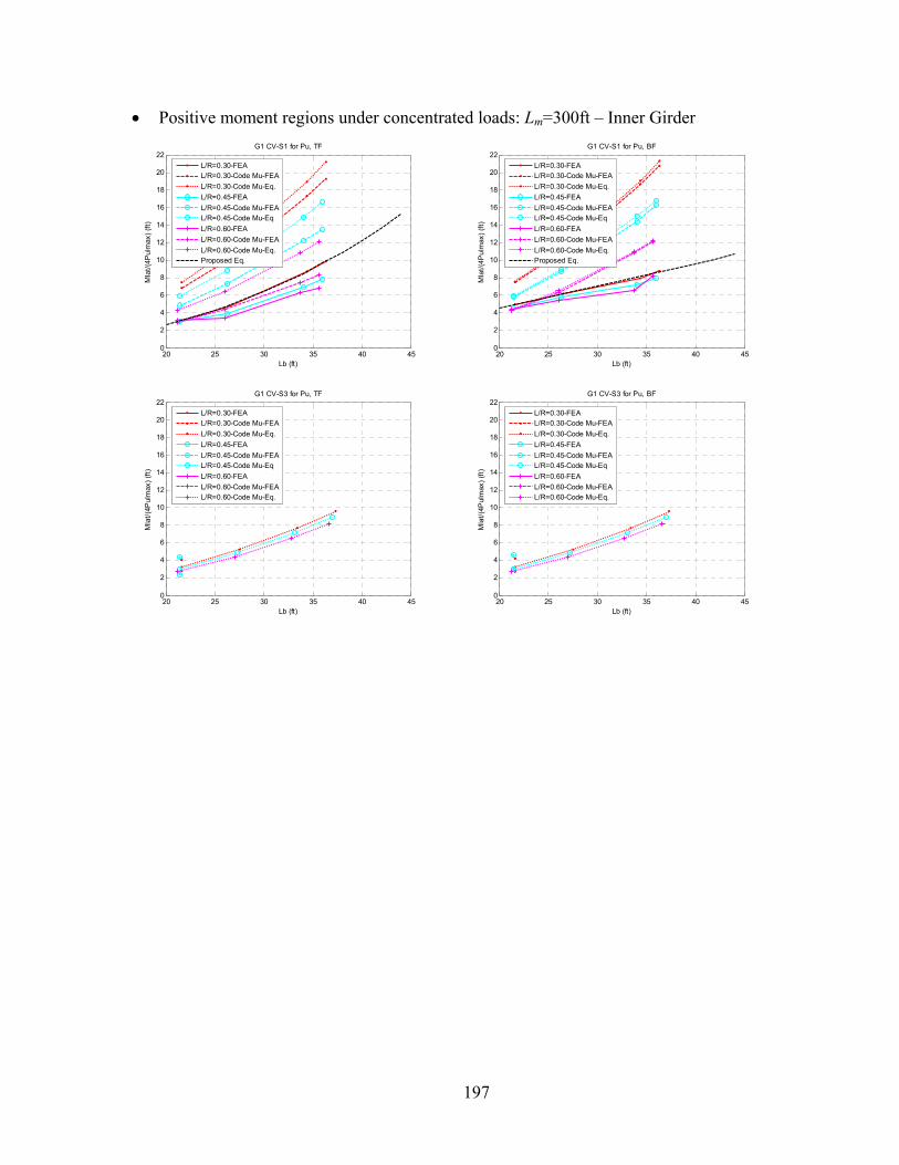
197
• Positive moment regions under concentrated loads: Lm=300ft – Inner Girder
20 25 30 35 40 450
2
4
6
8
10
12
14
16
18
20
22G1 CV-S1 for Pu, TF
Mla
t/(4P
ulm
ax) (
ft)
Lb (ft)
L/R=0.30-FEAL/R=0.30-Code Mu-FEAL/R=0.30-Code Mu-Eq.L/R=0.45-FEAL/R=0.45-Code Mu-FEAL/R=0.45-Code Mu-EqL/R=0.60-FEAL/R=0.60-Code Mu-FEAL/R=0.60-Code Mu-Eq.Proposed Eq.
20 25 30 35 40 450
2
4
6
8
10
12
14
16
18
20
22G1 CV-S1 for Pu, BF
Mla
t/(4P
ulm
ax) (
ft)
Lb (ft)
L/R=0.30-FEAL/R=0.30-Code Mu-FEAL/R=0.30-Code Mu-Eq.L/R=0.45-FEAL/R=0.45-Code Mu-FEAL/R=0.45-Code Mu-EqL/R=0.60-FEAL/R=0.60-Code Mu-FEAL/R=0.60-Code Mu-Eq.Proposed Eq.
20 25 30 35 40 450
2
4
6
8
10
12
14
16
18
20
22G1 CV-S3 for Pu, TF
Mla
t/(4P
ulm
ax) (
ft)
Lb (ft)
L/R=0.30-FEAL/R=0.30-Code Mu-FEAL/R=0.30-Code Mu-Eq.L/R=0.45-FEAL/R=0.45-Code Mu-FEAL/R=0.45-Code Mu-EqL/R=0.60-FEAL/R=0.60-Code Mu-FEAL/R=0.60-Code Mu-Eq.
20 25 30 35 40 450
2
4
6
8
10
12
14
16
18
20
22G1 CV-S3 for Pu, BF
Mla
t/(4P
ulm
ax) (
ft)
Lb (ft)
L/R=0.30-FEAL/R=0.30-Code Mu-FEAL/R=0.30-Code Mu-Eq.L/R=0.45-FEAL/R=0.45-Code Mu-FEAL/R=0.45-Code Mu-EqL/R=0.60-FEAL/R=0.60-Code Mu-FEAL/R=0.60-Code Mu-Eq.

198
• Negative moment regions: Lm=240ft
20 25 30 35 40 450
20
40
60
80
100
120G4 CV-S2 for wu, TF
Mla
t/wul
max
(ft2 )
Lb (ft)
L/R=0.30-FEAL/R=0.30-Code Mu-FEAL/R=0.30-Code Mu-Eq.L/R=0.45-FEAL/R=0.45-Code Mu-FEAL/R=0.45-Code Mu-EqL/R=0.60-FEAL/R=0.60-Code Mu-FEAL/R=0.60-Code Mu-Eq.Proposed Eq.
20 25 30 35 40 450
20
40
60
80
100
120G4 CV-S2 for wu, BF
Mla
t/wul
max
(ft2 )
Lb (ft)
L/R=0.30-FEAL/R=0.30-Code Mu-FEAL/R=0.30-Code Mu-Eq.L/R=0.45-FEAL/R=0.45-Code Mu-FEAL/R=0.45-Code Mu-EqL/R=0.60-FEAL/R=0.60-Code Mu-FEAL/R=0.60-Code Mu-Eq.Proposed Eq.
20 25 30 35 40 450
20
40
60
80
100
120G1 CV-S2 for wu, TF
Mla
t/wul
max
(ft2 )
Lb (ft)
L/R=0.30-FEAL/R=0.30-Code Mu-FEAL/R=0.30-Code Mu-Eq.L/R=0.45-FEAL/R=0.45-Code Mu-FEAL/R=0.45-Code Mu-EqL/R=0.60-FEAL/R=0.60-Code Mu-FEAL/R=0.60-Code Mu-Eq.Proposed Eq.
20 25 30 35 40 450
20
40
60
80
100
120G1 CV-S2 for wu, BF
Mla
t/wul
max
(ft2 )
Lb (ft)
L/R=0.30-FEAL/R=0.30-Code Mu-FEAL/R=0.30-Code Mu-Eq.L/R=0.45-FEAL/R=0.45-Code Mu-FEAL/R=0.45-Code Mu-EqL/R=0.60-FEAL/R=0.60-Code Mu-FEAL/R=0.60-Code Mu-Eq.Proposed Eq.

199
• Negative moment regions: Lm=300ft
20 25 30 35 40 450
20
40
60
80
100
120G4 CV-S2 for wu, TF
Mla
t/wul
max
(ft2 )
Lb (ft)
L/R=0.30-FEAL/R=0.30-Code Mu-FEAL/R=0.30-Code Mu-Eq.L/R=0.45-FEAL/R=0.45-Code Mu-FEAL/R=0.45-Code Mu-EqL/R=0.60-FEAL/R=0.60-Code Mu-FEAL/R=0.60-Code Mu-Eq.Proposed Eq.
20 25 30 35 40 450
20
40
60
80
100
120G4 CV-S2 for wu, BF
Mla
t/wul
max
(ft2 )
Lb (ft)
L/R=0.30-FEAL/R=0.30-Code Mu-FEAL/R=0.30-Code Mu-Eq.L/R=0.45-FEAL/R=0.45-Code Mu-FEAL/R=0.45-Code Mu-EqL/R=0.60-FEAL/R=0.60-Code Mu-FEAL/R=0.60-Code Mu-Eq.Proposed Eq.
20 25 30 35 40 450
20
40
60
80
100
120G1 CV-S2 for wu, TF
Mla
t/wul
max
(ft2 )
Lb (ft)
L/R=0.30-FEAL/R=0.30-Code Mu-FEAL/R=0.30-Code Mu-Eq.L/R=0.45-FEAL/R=0.45-Code Mu-FEAL/R=0.45-Code Mu-EqL/R=0.60-FEAL/R=0.60-Code Mu-FEAL/R=0.60-Code Mu-Eq.Proposed Eq.
20 25 30 35 40 450
20
40
60
80
100
120G1 CV-S2 for wu, BF
Mla
t/wul
max
(ft2 )
Lb (ft)
L/R=0.30-FEAL/R=0.30-Code Mu-FEAL/R=0.30-Code Mu-Eq.L/R=0.45-FEAL/R=0.45-Code Mu-FEAL/R=0.45-Code Mu-EqL/R=0.60-FEAL/R=0.60-Code Mu-FEAL/R=0.60-Code Mu-Eq.Proposed Eq.

200
Appendix C: Limit States for constructibility in Skewed
Bridges • Skewed bridges: Lb=25ft – Cross frames oriented perpendicular to the girders
G4 G1
0 0.05 0.1 0.15 0.2 0.25 0.3 0.35 0.4 0.45 0.5
-1
-0.5
0
0.5
1
G4 Lm=150ft, C1
Normalized distance (xi/Lt)
Dem
and/
Cap
acity
0 0.05 0.1 0.15 0.2 0.25 0.3 0.35 0.4 0.45 0.5
-1
-0.5
0
0.5
1
G1 Lm=150ft, C1
Normalized distance (xi/Lt)
Dem
and/
Cap
acity
0 0.05 0.1 0.15 0.2 0.25 0.3 0.35 0.4 0.45 0.5
-1
-0.5
0
0.5
1
G4 Lm=150ft, C2
Normalized distance (xi/Lt)
Dem
and/
Cap
acity
0 0.05 0.1 0.15 0.2 0.25 0.3 0.35 0.4 0.45 0.5
-1
-0.5
0
0.5
1
G1 Lm=150ft, C2
Normalized distance (xi/Lt)
Dem
and/
Cap
acity
0 0.05 0.1 0.15 0.2 0.25 0.3 0.35 0.4 0.45 0.5
-1
-0.5
0
0.5
1
G4 Lm=150ft, C3
Normalized distance (xi/Lt)
Dem
and/
Cap
acity
0 0.05 0.1 0.15 0.2 0.25 0.3 0.35 0.4 0.45 0.5
-1
-0.5
0
0.5
1
G1 Lm=150ft, C3
Normalized distance (xi/Lt)
Dem
and/
Cap
acity

201
0 0.05 0.1 0.15 0.2 0.25 0.3 0.35 0.4 0.45 0.5
-1
-0.5
0
0.5
1
G4 Lm=150ft, C4
Normalized distance (xi/Lt)
Dem
and/
Cap
acity
0 0.05 0.1 0.15 0.2 0.25 0.3 0.35 0.4 0.45 0.5
-1
-0.5
0
0.5
1
G1 Lm=150ft, C4
Normalized distance (xi/Lt)
Dem
and/
Cap
acity
0 0.05 0.1 0.15 0.2 0.25 0.3 0.35 0.4 0.45 0.5
-1
-0.5
0
0.5
1
G4 Lm=150ft, C5
Normalized distance (xi/Lt)
Dem
and/
Cap
acity
0 0.05 0.1 0.15 0.2 0.25 0.3 0.35 0.4 0.45 0.5
-1
-0.5
0
0.5
1
G1 Lm=150ft, C5
Normalized distance (xi/Lt)
Dem
and/
Cap
acity
TF: ST L/R=0.30 L/R=0.45 L/R=0.60
BF: ST L/R=0.30 L/R=0.45 L/R=0.60

202
• Skewed bridges: Lb=40ft – Cross frames oriented perpendicular to the girders G4 G2
0 0.05 0.1 0.15 0.2 0.25 0.3 0.35 0.4 0.45 0.5
-1
-0.5
0
0.5
1
G4 Lm=150ft, C1
Normalized distance (xi/Lt)
Dem
and/
Cap
acity
0 0.05 0.1 0.15 0.2 0.25 0.3 0.35 0.4 0.45 0.5
-1
-0.5
0
0.5
1
G1 Lm=150ft, C1
Normalized distance (xi/Lt)
Dem
and/
Cap
acity
0 0.05 0.1 0.15 0.2 0.25 0.3 0.35 0.4 0.45 0.5
-1
-0.5
0
0.5
1
G4 Lm=150ft, C2
Normalized distance (xi/Lt)
Dem
and/
Cap
acity
0 0.05 0.1 0.15 0.2 0.25 0.3 0.35 0.4 0.45 0.5
-1
-0.5
0
0.5
1
G1 Lm=150ft, C2
Normalized distance (xi/Lt)
Dem
and/
Cap
acity
0 0.05 0.1 0.15 0.2 0.25 0.3 0.35 0.4 0.45 0.5
-1
-0.5
0
0.5
1
G4 Lm=150ft, C3
Normalized distance (xi/Lt)
Dem
and/
Cap
acity
0 0.05 0.1 0.15 0.2 0.25 0.3 0.35 0.4 0.45 0.5
-1
-0.5
0
0.5
1
G1 Lm=150ft, C3
Normalized distance (xi/Lt)
Dem
and/
Cap
acity

203
0 0.05 0.1 0.15 0.2 0.25 0.3 0.35 0.4 0.45 0.5
-1
-0.5
0
0.5
1
G4 Lm=150ft, C4
Normalized distance (xi/Lt)
Dem
and/
Cap
acity
0 0.05 0.1 0.15 0.2 0.25 0.3 0.35 0.4 0.45 0.5
-1
-0.5
0
0.5
1
G1 Lm=150ft, C4
Normalized distance (xi/Lt)
Dem
and/
Cap
acity
0 0.05 0.1 0.15 0.2 0.25 0.3 0.35 0.4 0.45 0.5
-1
-0.5
0
0.5
1
G4 Lm=150ft, C5
Normalized distance (xi/Lt)
Dem
and/
Cap
acity
0 0.05 0.1 0.15 0.2 0.25 0.3 0.35 0.4 0.45 0.5
-1
-0.5
0
0.5
1
G1 Lm=150ft, C5
Normalized distance (xi/Lt)
Dem
and/
Cap
acity
TF: ST L/R=0.30 L/R=0.45 L/R=0.60
BF: ST L/R=0.30 L/R=0.45 L/R=0.60

204
• Skewed bridges: Lb=40ft – Cross frames oriented parallel to the supports G4 G1
0 0.05 0.1 0.15 0.2 0.25 0.3 0.35 0.4 0.45 0.5
-1
-0.5
0
0.5
1
G4 Lm=150ft, C1
Normalized distance (xi/Lt)
Dem
and/
Cap
acity
0 0.05 0.1 0.15 0.2 0.25 0.3 0.35 0.4 0.45 0.5
-1
-0.5
0
0.5
1
G1 Lm=150ft, C1
Normalized distance (xi/Lt)
Dem
and/
Cap
acity
0 0.05 0.1 0.15 0.2 0.25 0.3 0.35 0.4 0.45 0.5
-1
-0.5
0
0.5
1
G4 Lm=150ft, C2
Normalized distance (xi/Lt)
Dem
and/
Cap
acity
0 0.05 0.1 0.15 0.2 0.25 0.3 0.35 0.4 0.45 0.5
-1
-0.5
0
0.5
1
G1 Lm=150ft, C2
Normalized distance (xi/Lt)
Dem
and/
Cap
acity
0 0.05 0.1 0.15 0.2 0.25 0.3 0.35 0.4 0.45 0.5
-1
-0.5
0
0.5
1
G4 Lm=150ft, C3
Normalized distance (xi/Lt)
Dem
and/
Cap
acity
0 0.05 0.1 0.15 0.2 0.25 0.3 0.35 0.4 0.45 0.5
-1
-0.5
0
0.5
1
G1 Lm=150ft, C3
Normalized distance (xi/Lt)
Dem
and/
Cap
acity

205
0 0.05 0.1 0.15 0.2 0.25 0.3 0.35 0.4 0.45 0.5
-1
-0.5
0
0.5
1
G4 Lm=150ft, C4
Normalized distance (xi/Lt)
Dem
and/
Cap
acity
0 0.05 0.1 0.15 0.2 0.25 0.3 0.35 0.4 0.45 0.5
-1
-0.5
0
0.5
1
G1 Lm=150ft, C4
Normalized distance (xi/Lt)
Dem
and/
Cap
acity
0 0.05 0.1 0.15 0.2 0.25 0.3 0.35 0.4 0.45 0.5
-1
-0.5
0
0.5
1
G4 Lm=150ft, C5
Normalized distance (xi/Lt)
Dem
and/
Cap
acity
0 0.05 0.1 0.15 0.2 0.25 0.3 0.35 0.4 0.45 0.5
-1
-0.5
0
0.5
1
G1 Lm=150ft, C5
Normalized distance (xi/Lt)
Dem
and/
Cap
acity
TF: ST L/R=0.30 L/R=0.45 L/R=0.60
BF: ST L/R=0.30 L/R=0.45 L/R=0.60

206
• Skewed bridges: Lb=25ft – Cross frames oriented perpendicular to the girders
0 0.05 0.1 0.15 0.2 0.25 0.3 0.35 0.4 0.45 0.5-0.4
-0.3
-0.2
-0.1
0
0.1
0.2
0.3
0.4G4 Lm=150ft, C2, TF
Normalized distance (xi/Lt)
fb/F
yf
0 0.05 0.1 0.15 0.2 0.25 0.3 0.35 0.4 0.45 0.5
-0.4
-0.3
-0.2
-0.1
0
0.1
0.2
0.3
0.4G1 Lm=150ft, C2, TF
Normalized distance (xi/Lt)
fb/F
yf
0 0.05 0.1 0.15 0.2 0.25 0.3 0.35 0.4 0.45 0.5
-0.6
-0.4
-0.2
0
0.2
0.4
0.6
G4 Lm=150ft, C2, TF
Normalized distance (xi/Lt)
fl / F
yf
0 0.05 0.1 0.15 0.2 0.25 0.3 0.35 0.4 0.45 0.5
-0.6
-0.4
-0.2
0
0.2
0.4
0.6
G1 Lm=150ft, C2, TF
Normalized distance (xi/Lt)
fl / F
yf
ST
L/R=0.30
L/R=0.45
L/R=0.60

207
• Skewed bridges: Lb=40ft – Cross frames oriented perpendicular to the girders
0 0.05 0.1 0.15 0.2 0.25 0.3 0.35 0.4 0.45 0.5-0.4
-0.3
-0.2
-0.1
0
0.1
0.2
0.3
0.4G4 Lm=150ft, C2, TF
Normalized distance (xi/Lt)
fb/F
yf
0 0.05 0.1 0.15 0.2 0.25 0.3 0.35 0.4 0.45 0.5
-0.4
-0.3
-0.2
-0.1
0
0.1
0.2
0.3
0.4G1 Lm=150ft, C2, TF
Normalized distance (xi/Lt)
fb/F
yf
0 0.05 0.1 0.15 0.2 0.25 0.3 0.35 0.4 0.45 0.5
-0.6
-0.4
-0.2
0
0.2
0.4
0.6
G4 Lm=150ft, C2, TF
Normalized distance (xi/Lt)
fl / F
yf
0 0.05 0.1 0.15 0.2 0.25 0.3 0.35 0.4 0.45 0.5
-0.6
-0.4
-0.2
0
0.2
0.4
0.6
G1 Lm=150ft, C2, TF
Normalized distance (xi/Lt)
fl / F
yf
ST
L/R=0.30
L/R=0.45
L/R=0.60

208
• Skewed bridges: Lb=40ft – Cross frames oriented parallel to the supports
0 0.05 0.1 0.15 0.2 0.25 0.3 0.35 0.4 0.45 0.5-0.4
-0.3
-0.2
-0.1
0
0.1
0.2
0.3
0.4G4 Lm=150ft, C2, TF
Normalized distance (xi/Lt)
fb/F
yf
0 0.05 0.1 0.15 0.2 0.25 0.3 0.35 0.4 0.45 0.5
-0.4
-0.3
-0.2
-0.1
0
0.1
0.2
0.3
0.4G1 Lm=150ft, C2, TF
Normalized distance (xi/Lt)
fb/F
yf
0 0.05 0.1 0.15 0.2 0.25 0.3 0.35 0.4 0.45 0.5
-0.6
-0.4
-0.2
0
0.2
0.4
0.6
G4 Lm=150ft, C2, TF
Normalized distance (xi/Lt)
fl / F
yf
0 0.05 0.1 0.15 0.2 0.25 0.3 0.35 0.4 0.45 0.5
-0.6
-0.4
-0.2
0
0.2
0.4
0.6
G1 Lm=150ft, C2, TF
Normalized distance (xi/Lt)
fl / F
yf
ST
L/R=0.30
L/R=0.45
L/R=0.60

209
• Skewed bridges: Lm=150ft – Section 1
25 27 32 370
0.2
0.4
0.6
0.8
1
1.2
G4 Lm=150ft, TF S1D
/C m
ax
25 27 32 370
1
2
3
4
5
Cas
ting
#
25 27 32 370
1
2
3
4
5
Lb (ft)
Lim
it S
tate
ST SK30 SK45 SK60
25 27 32 370
0.2
0.4
0.6
0.8
1
1.2
G4 Lm=150ft, BF S1
D/C
max
25 27 32 370
1
2
3
4
5
Cas
ting
#
25 27 32 370
1
2
3
4
5
Lb (ft)
Lim
it S
tate
ST SK30 SK45 SK60
25 27 32 370
0.2
0.4
0.6
0.8
1
1.2
G1 Lm=150ft, TF S1
D/C
max
25 27 32 370
1
2
3
4
5
Cas
ting
#
25 27 32 370
1
2
3
4
5
Lb (ft)
Lim
it S
tate
ST SK30 SK45 SK60
25 27 32 370
0.2
0.4
0.6
0.8
1
1.2
G1 Lm=150ft, BF S1
D/C
max
25 27 32 370
1
2
3
4
5
Cas
ting
#
25 27 32 370
1
2
3
4
5
Lb (ft)
Lim
it S
tate
ST SK30 SK45 SK60

210
• Skewed bridges: Lm=150ft – Section 2
20 21 27 350
0.2
0.4
0.6
0.8
1
1.2
G4 Lm=150ft, TF S2D
/C m
ax
20 21 27 350
1
2
3
4
5
Cas
ting
#
20 21 27 350
1
2
3
4
5
Lb (ft)
Lim
it S
tate
ST SK30 SK45 SK60
20 21 27 350
0.2
0.4
0.6
0.8
1
1.2
G4 Lm=150ft, BF S2
D/C
max
20 21 27 350
1
2
3
4
5
Cas
ting
#
20 21 27 350
1
2
3
4
5
Lb (ft)
Lim
it S
tate
ST SK30 SK45 SK60
20 21 27 350
0.2
0.4
0.6
0.8
1
1.2
G1 Lm=150ft, TF S2
D/C
max
20 21 27 350
1
2
3
4
5
Cas
ting
#
20 21 27 350
1
2
3
4
5
Lb (ft)
Lim
it S
tate
ST SK30 SK45 SK60
20 21 27 350
0.2
0.4
0.6
0.8
1
1.2
G1 Lm=150ft, BF S2
D/C
max
20 21 27 350
1
2
3
4
5
Cas
ting
#
20 21 27 350
1
2
3
4
5
Lb (ft)
Lim
it S
tate
ST SK30 SK45 SK60

211
• Skewed bridges: Lm=150ft – Section 3
22 27 32 400
0.2
0.4
0.6
0.8
1
1.2
G4 Lm=150ft, TF S3D
/C m
ax
22 27 32 400
1
2
3
4
5
Cas
ting
#
22 27 32 400
1
2
3
4
5
Lb (ft)
Lim
it S
tate
ST SK30 SK45 SK60
22 27 32 400
0.2
0.4
0.6
0.8
1
1.2
G4 Lm=150ft, BF S3
D/C
max
22 27 32 400
1
2
3
4
5
Cas
ting
#
22 27 32 400
1
2
3
4
5
Lb (ft)
Lim
it S
tate
ST SK30 SK45 SK60
22 27 32 400
0.2
0.4
0.6
0.8
1
1.2
G1 Lm=150ft, TF S3
D/C
max
22 27 32 400
1
2
3
4
5
Cas
ting
#
22 27 32 400
1
2
3
4
5
Lb (ft)
Lim
it S
tate
ST SK30 SK45 SK60
22 27 32 400
0.2
0.4
0.6
0.8
1
1.2
G1 Lm=150ft, BF S3
D/C
max
22 27 32 400
1
2
3
4
5
Cas
ting
#
22 27 32 400
1
2
3
4
5
Lb (ft)
Lim
it S
tate
ST SK30 SK45 SK60

212
Appendix D: Limit States for constructibility in Curved
Bridges • Curved bridges: Lb=25ft
G4 G1
0 0.05 0.1 0.15 0.2 0.25 0.3 0.35 0.4 0.45 0.5
-1
-0.5
0
0.5
1
G4 Lm=150ft, C1
Normalized distance (xi/Lt)
Dem
and/
Cap
acity
0 0.05 0.1 0.15 0.2 0.25 0.3 0.35 0.4 0.45 0.5
-1
-0.5
0
0.5
1
G1 Lm=150ft, C1
Normalized distance (xi/Lt)
Dem
and/
Cap
acity
0 0.05 0.1 0.15 0.2 0.25 0.3 0.35 0.4 0.45 0.5
-1
-0.5
0
0.5
1
G4 Lm=150ft, C2
Normalized distance (xi/Lt)
Dem
and/
Cap
acity
0 0.05 0.1 0.15 0.2 0.25 0.3 0.35 0.4 0.45 0.5
-1
-0.5
0
0.5
1
G1 Lm=150ft, C2
Normalized distance (xi/Lt)
Dem
and/
Cap
acity
0 0.05 0.1 0.15 0.2 0.25 0.3 0.35 0.4 0.45 0.5
-1
-0.5
0
0.5
1
G4 Lm=150ft, C3
Normalized distance (xi/Lt)
Dem
and/
Cap
acity
0 0.05 0.1 0.15 0.2 0.25 0.3 0.35 0.4 0.45 0.5
-1
-0.5
0
0.5
1
G1 Lm=150ft, C3
Normalized distance (xi/Lt)
Dem
and/
Cap
acity
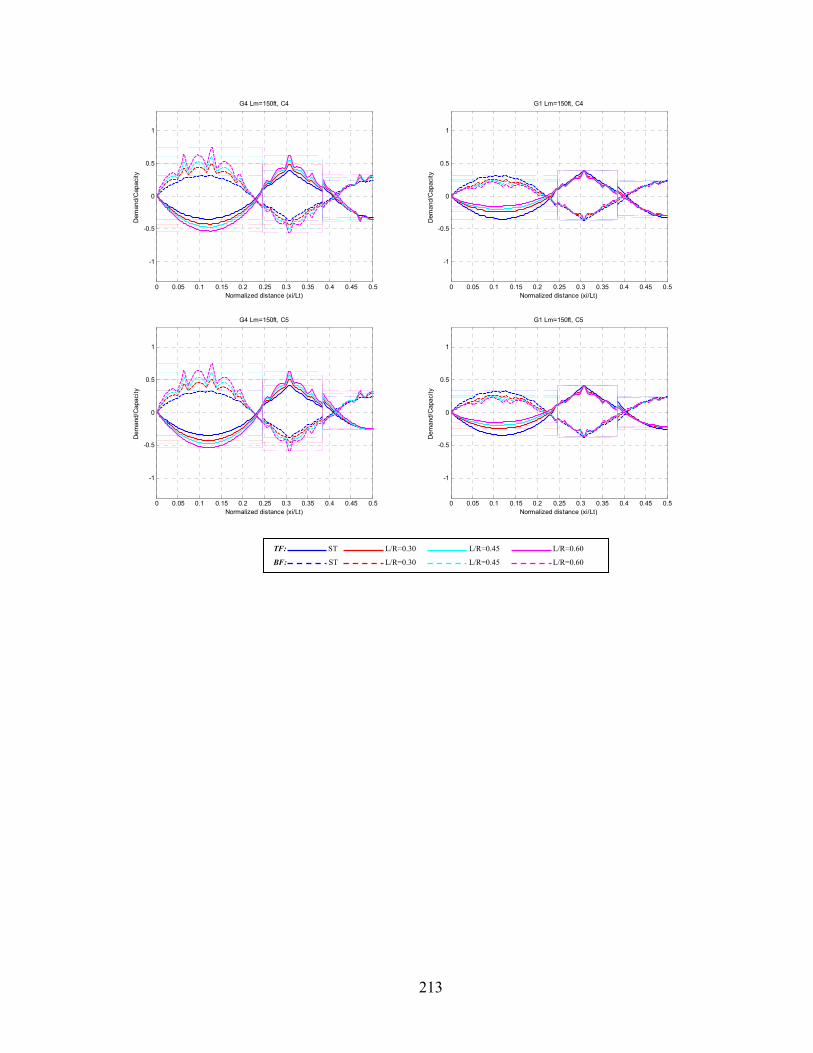
213
0 0.05 0.1 0.15 0.2 0.25 0.3 0.35 0.4 0.45 0.5
-1
-0.5
0
0.5
1
G4 Lm=150ft, C4
Normalized distance (xi/Lt)
Dem
and/
Cap
acity
0 0.05 0.1 0.15 0.2 0.25 0.3 0.35 0.4 0.45 0.5
-1
-0.5
0
0.5
1
G1 Lm=150ft, C4
Normalized distance (xi/Lt)
Dem
and/
Cap
acity
0 0.05 0.1 0.15 0.2 0.25 0.3 0.35 0.4 0.45 0.5
-1
-0.5
0
0.5
1
G4 Lm=150ft, C5
Normalized distance (xi/Lt)
Dem
and/
Cap
acity
0 0.05 0.1 0.15 0.2 0.25 0.3 0.35 0.4 0.45 0.5
-1
-0.5
0
0.5
1
G1 Lm=150ft, C5
Normalized distance (xi/Lt)
Dem
and/
Cap
acity
TF: ST L/R=0.30 L/R=0.45 L/R=0.60
BF: ST L/R=0.30 L/R=0.45 L/R=0.60

214
• Curved bridges: Lb=25ft
0 0.05 0.1 0.15 0.2 0.25 0.3 0.35 0.4 0.45 0.5-0.8
-0.6
-0.4
-0.2
0
0.2
0.4
0.6G4 Lm=150ft, C2, TF
Normalized distance (xi/Lt)
fb/F
yf
0 0.05 0.1 0.15 0.2 0.25 0.3 0.35 0.4 0.45 0.5
-0.4
-0.3
-0.2
-0.1
0
0.1
0.2
0.3
0.4G1 Lm=150ft, C2, TF
Normalized distance (xi/Lt)
fb/F
yf
0 0.05 0.1 0.15 0.2 0.25 0.3 0.35 0.4 0.45 0.5
-0.6
-0.4
-0.2
0
0.2
0.4
0.6
G4 Lm=150ft, C2, TF
Normalized distance (xi/Lt)
fl / F
yf
0 0.05 0.1 0.15 0.2 0.25 0.3 0.35 0.4 0.45 0.5
-0.6
-0.4
-0.2
0
0.2
0.4
0.6
G1 Lm=150ft, C2, TF
Normalized distance (xi/Lt)
fl / F
yf
ST
L/R=0.30
L/R=0.45
L/R=0.60

215
• Curved bridges: Lb=40ft G4 G1
0 0.05 0.1 0.15 0.2 0.25 0.3 0.35 0.4 0.45 0.5
-1
-0.5
0
0.5
1
G4 Lm=150ft, C1
Normalized distance (xi/Lt)
Dem
and/
Cap
acity
0 0.05 0.1 0.15 0.2 0.25 0.3 0.35 0.4 0.45 0.5
-1
-0.5
0
0.5
1
G1 Lm=150ft, C1
Normalized distance (xi/Lt)
Dem
and/
Cap
acity
0 0.05 0.1 0.15 0.2 0.25 0.3 0.35 0.4 0.45 0.5
-1
-0.5
0
0.5
1
G4 Lm=150ft, C2
Normalized distance (xi/Lt)
Dem
and/
Cap
acity
0 0.05 0.1 0.15 0.2 0.25 0.3 0.35 0.4 0.45 0.5
-1
-0.5
0
0.5
1
G1 Lm=150ft, C2
Normalized distance (xi/Lt)
Dem
and/
Cap
acity
0 0.05 0.1 0.15 0.2 0.25 0.3 0.35 0.4 0.45 0.5
-1
-0.5
0
0.5
1
G4 Lm=150ft, C3
Normalized distance (xi/Lt)
Dem
and/
Cap
acity
0 0.05 0.1 0.15 0.2 0.25 0.3 0.35 0.4 0.45 0.5
-1
-0.5
0
0.5
1
G1 Lm=150ft, C3
Normalized distance (xi/Lt)
Dem
and/
Cap
acity

216
0 0.05 0.1 0.15 0.2 0.25 0.3 0.35 0.4 0.45 0.5
-1
-0.5
0
0.5
1
G4 Lm=150ft, C4
Normalized distance (xi/Lt)
Dem
and/
Cap
acity
0 0.05 0.1 0.15 0.2 0.25 0.3 0.35 0.4 0.45 0.5
-1
-0.5
0
0.5
1
G1 Lm=150ft, C4
Normalized distance (xi/Lt)
Dem
and/
Cap
acity
0 0.05 0.1 0.15 0.2 0.25 0.3 0.35 0.4 0.45 0.5
-1
-0.5
0
0.5
1
G4 Lm=150ft, C5
Normalized distance (xi/Lt)
Dem
and/
Cap
acity
0 0.05 0.1 0.15 0.2 0.25 0.3 0.35 0.4 0.45 0.5
-1
-0.5
0
0.5
1
G1 Lm=150ft, C5
Normalized distance (xi/Lt)
Dem
and/
Cap
acity
TF: ST L/R=0.30 L/R=0.45 L/R=0.60
BF: ST L/R=0.30 L/R=0.45 L/R=0.60

217
• Curved bridges: Lb=40ft
0 0.05 0.1 0.15 0.2 0.25 0.3 0.35 0.4 0.45 0.5-0.8
-0.6
-0.4
-0.2
0
0.2
0.4
0.6G4 Lm=150ft, C2, TF
Normalized distance (xi/Lt)
fb/F
yf
0 0.05 0.1 0.15 0.2 0.25 0.3 0.35 0.4 0.45 0.5
-0.4
-0.3
-0.2
-0.1
0
0.1
0.2
0.3
0.4G1 Lm=150ft, C2, TF
Normalized distance (xi/Lt)
fb/F
yf
0 0.05 0.1 0.15 0.2 0.25 0.3 0.35 0.4 0.45 0.5
-0.6
-0.4
-0.2
0
0.2
0.4
0.6
G4 Lm=150ft, C2, TF
Normalized distance (xi/Lt)
fl / F
yf
0 0.05 0.1 0.15 0.2 0.25 0.3 0.35 0.4 0.45 0.5
-0.6
-0.4
-0.2
0
0.2
0.4
0.6
G1 Lm=150ft, C2, TF
Normalized distance (xi/Lt)
fl / F
yf
ST
L/R=0.30
L/R=0.45
L/R=0.60

218
• Curved bridges: Lm=150ft – Section 1
25 27 32 370
0.2
0.4
0.6
0.8
1
1.2
G4 Lm=150ft, TF S1D
/C m
ax
25 27 32 370
1
2
3
4
5
Cas
ting
#
25 27 32 370
1
2
3
4
5
Lb (ft)
Lim
it S
tate
ST CV30 CV45 CV60
25 27 32 370
0.2
0.4
0.6
0.8
1
1.2
G4 Lm=150ft, BF S1
D/C
max
25 27 32 370
1
2
3
4
5
Cas
ting
#
25 27 32 370
1
2
3
4
5
Lb (ft)
Lim
it S
tate
ST CV30 CV45 CV60
25 27 32 370
0.2
0.4
0.6
0.8
1
1.2
G1 Lm=150ft, TF S1
D/C
max
25 27 32 370
1
2
3
4
5
Cas
ting
#
25 27 32 370
1
2
3
4
5
Lb (ft)
Lim
it S
tate
ST CV30 CV45 CV60
25 27 32 370
0.2
0.4
0.6
0.8
1
1.2
G1 Lm=150ft, BF S1D
/C m
ax
25 27 32 370
1
2
3
4
5
Cas
ting
#
25 27 32 370
1
2
3
4
5
Lb (ft)
Lim
it S
tate
ST CV30 CV45 CV60

219
• Curved bridges: Lm=150ft – Section 2
20 21 27 350
0.2
0.4
0.6
0.8
1
1.2
G4 Lm=150ft, TF S2D
/C m
ax
20 21 27 350
1
2
3
4
5
Cas
ting
#
20 21 27 350
1
2
3
4
5
Lb (ft)
Lim
it S
tate
ST CV30 CV45 CV60
20 21 27 350
0.2
0.4
0.6
0.8
1
1.2
G4 Lm=150ft, BF S2
D/C
max
20 21 27 350
1
2
3
4
5
Cas
ting
#
20 21 27 350
1
2
3
4
5
Lb (ft)
Lim
it S
tate
ST CV30 CV45 CV60
20 21 27 350
0.2
0.4
0.6
0.8
1
1.2
G1 Lm=150ft, TF S2
D/C
max
20 21 27 350
1
2
3
4
5
Cas
ting
#
20 21 27 350
1
2
3
4
5
Lb (ft)
Lim
it S
tate
ST CV30 CV45 CV60
20 21 27 350
0.2
0.4
0.6
0.8
1
1.2
G1 Lm=150ft, BF S2
D/C
max
20 21 27 350
1
2
3
4
5
Cas
ting
#
20 21 27 350
1
2
3
4
5
Lb (ft)
Lim
it S
tate
ST CV30 CV45 CV60

220
• Curved bridges: Lm=150ft – Section 3
22 27 32 400
0.2
0.4
0.6
0.8
1
1.2
G4 Lm=150ft, TF S3D
/C m
ax
22 27 32 400
1
2
3
4
5
Cas
ting
#
22 27 32 400
1
2
3
4
5
Lb (ft)
Lim
it S
tate
ST CV30 CV45 CV60
22 27 32 400
0.2
0.4
0.6
0.8
1
1.2
G4 Lm=150ft, BF S3
D/C
max
22 27 32 400
1
2
3
4
5
Cas
ting
#
22 27 32 400
1
2
3
4
5
Lb (ft)
Lim
it S
tate
ST CV30 CV45 CV60
22 27 32 400
0.2
0.4
0.6
0.8
1
1.2
G1 Lm=150ft, TF S3
D/C
max
22 27 32 400
1
2
3
4
5
Cas
ting
#
22 27 32 400
1
2
3
4
5
Lb (ft)
Lim
it S
tate
ST CV30 CV45 CV60
22 27 32 400
0.2
0.4
0.6
0.8
1
1.2
G1 Lm=150ft, BF S3D
/C m
ax
22 27 32 400
1
2
3
4
5
Cas
ting
#
22 27 32 400
1
2
3
4
5
Lb (ft)
Lim
it S
tate
ST CV30 CV45 CV60

221
Appendix E: Fragility Curves in Skewed Bridges • Skewed bridges: θ=45° - S1
10 20 30 40 50 60 70 80 90 1000
0.1
0.2
0.3
0.4
0.5
0.6
0.7
0.8
0.9
1S1 - TF - P
Lb (ft)
Pf
Lm=150ft, LS1Lm=150ft, LS2Lm=150ft, LS6Lm=240ft, LS1Lm=240ft, LS2Lm=240ft, LS6Lm=300ft, LS1Lm=300ft, LS2Lm=300ft, LS6
10 20 30 40 50 60 70 80 90 100-0.5
0
0.5
1
1.5
2
2.5
3
3.5
4
4.5
5S1 - TF - P
Lb (ft)
β
Lm=150ft, LS1Lm=150ft, LS2Lm=150ft, LS6Lm=240ft, LS1Lm=240ft, LS2Lm=240ft, LS6Lm=300ft, LS1Lm=300ft, LS2Lm=300ft, LS6Code
10 20 30 40 50 60 70 80 90 1000
0.1
0.2
0.3
0.4
0.5
0.6
0.7
0.8
0.9
1S1 - TF - w
Lb (ft)
Pf
Lm=150ft, LS1Lm=150ft, LS2Lm=150ft, LS6Lm=240ft, LS1Lm=240ft, LS2Lm=240ft, LS6Lm=300ft, LS1Lm=300ft, LS2Lm=300ft, LS6
10 20 30 40 50 60 70 80 90 100-0.5
0
0.5
1
1.5
2
2.5
3
3.5
4
4.5
5S1 - TF - w
Lb (ft)
βLm=150ft, LS1Lm=150ft, LS2Lm=150ft, LS6Lm=240ft, LS1Lm=240ft, LS2Lm=240ft, LS6Lm=300ft, LS1Lm=300ft, LS2Lm=300ft, LS6Code

222
• Skewed bridges: θ=45° - S3
10 20 30 40 50 60 70 80 90 1000
0.1
0.2
0.3
0.4
0.5
0.6
0.7
0.8
0.9
1S3 - TF - P
Lb (ft)
Pf
Lm=150ft, LS1Lm=150ft, LS2Lm=150ft, LS6Lm=240ft, LS1Lm=240ft, LS2Lm=240ft, LS6Lm=300ft, LS1Lm=300ft, LS2Lm=300ft, LS6
10 20 30 40 50 60 70 80 90 100-0.5
0
0.5
1
1.5
2
2.5
3
3.5
4
4.5
5S3 - TF - P
Lb (ft)
β
Lm=150ft, LS1Lm=150ft, LS2Lm=150ft, LS6Lm=240ft, LS1Lm=240ft, LS2Lm=240ft, LS6Lm=300ft, LS1Lm=300ft, LS2Lm=300ft, LS6Code
10 20 30 40 50 60 70 80 90 1000
0.1
0.2
0.3
0.4
0.5
0.6
0.7
0.8
0.9
1S3 - TF - w
Lb (ft)
Pf
Lm=150ft, LS1Lm=150ft, LS2Lm=150ft, LS6Lm=240ft, LS1Lm=240ft, LS2Lm=240ft, LS6Lm=300ft, LS1Lm=300ft, LS2Lm=300ft, LS6
10 20 30 40 50 60 70 80 90 100-0.5
0
0.5
1
1.5
2
2.5
3
3.5
4
4.5
5S3 - TF - w
Lb (ft)
βLm=150ft, LS1Lm=150ft, LS2Lm=150ft, LS6Lm=240ft, LS1Lm=240ft, LS2Lm=240ft, LS6Lm=300ft, LS1Lm=300ft, LS2Lm=300ft, LS6Code
• Skewed bridges: θ=45° - S2
10 20 30 40 50 60 70 80 90 1000
0.1
0.2
0.3
0.4
0.5
0.6
0.7
0.8
0.9
1S2 - BF - w
Lb (ft)
Pf
Lm=150ft, LS1Lm=150ft, LS2Lm=150ft, LS6Lm=240ft, LS1Lm=240ft, LS2Lm=240ft, LS6Lm=300ft, LS1Lm=300ft, LS2Lm=300ft, LS6
10 20 30 40 50 60 70 80 90 100-0.5
0
0.5
1
1.5
2
2.5
3
3.5
4
4.5
5S2 - BF - w
Lb (ft)
β
Lm=150ft, LS1Lm=150ft, LS2Lm=150ft, LS6Lm=240ft, LS1Lm=240ft, LS2Lm=240ft, LS6Lm=300ft, LS1Lm=300ft, LS2Lm=300ft, LS6Code

223
• Skewed bridges: θ=60° - S1
10 20 30 40 50 60 70 80 90 1000
0.1
0.2
0.3
0.4
0.5
0.6
0.7
0.8
0.9
1S1 - TF - P
Lb (ft)
Pf
Lm=150ft, LS1Lm=150ft, LS2Lm=150ft, LS6Lm=240ft, LS1Lm=240ft, LS2Lm=240ft, LS6Lm=300ft, LS1Lm=300ft, LS2Lm=300ft, LS6
10 20 30 40 50 60 70 80 90 100-0.5
0
0.5
1
1.5
2
2.5
3
3.5
4
4.5
5S1 - TF - P
Lb (ft)
β
Lm=150ft, LS1Lm=150ft, LS2Lm=150ft, LS6Lm=240ft, LS1Lm=240ft, LS2Lm=240ft, LS6Lm=300ft, LS1Lm=300ft, LS2Lm=300ft, LS6Code
10 20 30 40 50 60 70 80 90 1000
0.1
0.2
0.3
0.4
0.5
0.6
0.7
0.8
0.9
1S1 - TF - w
Lb (ft)
Pf
Lm=150ft, LS1Lm=150ft, LS2Lm=150ft, LS6Lm=240ft, LS1Lm=240ft, LS2Lm=240ft, LS6Lm=300ft, LS1Lm=300ft, LS2Lm=300ft, LS6
10 20 30 40 50 60 70 80 90 100-0.5
0
0.5
1
1.5
2
2.5
3
3.5
4
4.5
5S1 - TF - w
Lb (ft)
β
Lm=150ft, LS1Lm=150ft, LS2Lm=150ft, LS6Lm=240ft, LS1Lm=240ft, LS2Lm=240ft, LS6Lm=300ft, LS1Lm=300ft, LS2Lm=300ft, LS6Code
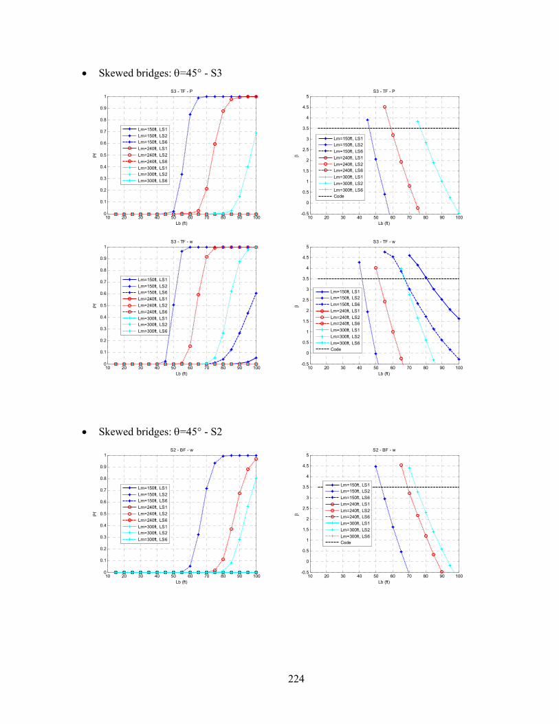
224
• Skewed bridges: θ=45° - S3
10 20 30 40 50 60 70 80 90 1000
0.1
0.2
0.3
0.4
0.5
0.6
0.7
0.8
0.9
1S3 - TF - P
Lb (ft)
Pf
Lm=150ft, LS1Lm=150ft, LS2Lm=150ft, LS6Lm=240ft, LS1Lm=240ft, LS2Lm=240ft, LS6Lm=300ft, LS1Lm=300ft, LS2Lm=300ft, LS6
10 20 30 40 50 60 70 80 90 100-0.5
0
0.5
1
1.5
2
2.5
3
3.5
4
4.5
5S3 - TF - P
Lb (ft)
β
Lm=150ft, LS1Lm=150ft, LS2Lm=150ft, LS6Lm=240ft, LS1Lm=240ft, LS2Lm=240ft, LS6Lm=300ft, LS1Lm=300ft, LS2Lm=300ft, LS6Code
10 20 30 40 50 60 70 80 90 1000
0.1
0.2
0.3
0.4
0.5
0.6
0.7
0.8
0.9
1S3 - TF - w
Lb (ft)
Pf
Lm=150ft, LS1Lm=150ft, LS2Lm=150ft, LS6Lm=240ft, LS1Lm=240ft, LS2Lm=240ft, LS6Lm=300ft, LS1Lm=300ft, LS2Lm=300ft, LS6
10 20 30 40 50 60 70 80 90 100-0.5
0
0.5
1
1.5
2
2.5
3
3.5
4
4.5
5S3 - TF - w
Lb (ft)
βLm=150ft, LS1Lm=150ft, LS2Lm=150ft, LS6Lm=240ft, LS1Lm=240ft, LS2Lm=240ft, LS6Lm=300ft, LS1Lm=300ft, LS2Lm=300ft, LS6Code
• Skewed bridges: θ=45° - S2
10 20 30 40 50 60 70 80 90 1000
0.1
0.2
0.3
0.4
0.5
0.6
0.7
0.8
0.9
1S2 - BF - w
Lb (ft)
Pf
Lm=150ft, LS1Lm=150ft, LS2Lm=150ft, LS6Lm=240ft, LS1Lm=240ft, LS2Lm=240ft, LS6Lm=300ft, LS1Lm=300ft, LS2Lm=300ft, LS6
10 20 30 40 50 60 70 80 90 100-0.5
0
0.5
1
1.5
2
2.5
3
3.5
4
4.5
5S2 - BF - w
Lb (ft)
β
Lm=150ft, LS1Lm=150ft, LS2Lm=150ft, LS6Lm=240ft, LS1Lm=240ft, LS2Lm=240ft, LS6Lm=300ft, LS1Lm=300ft, LS2Lm=300ft, LS6Code
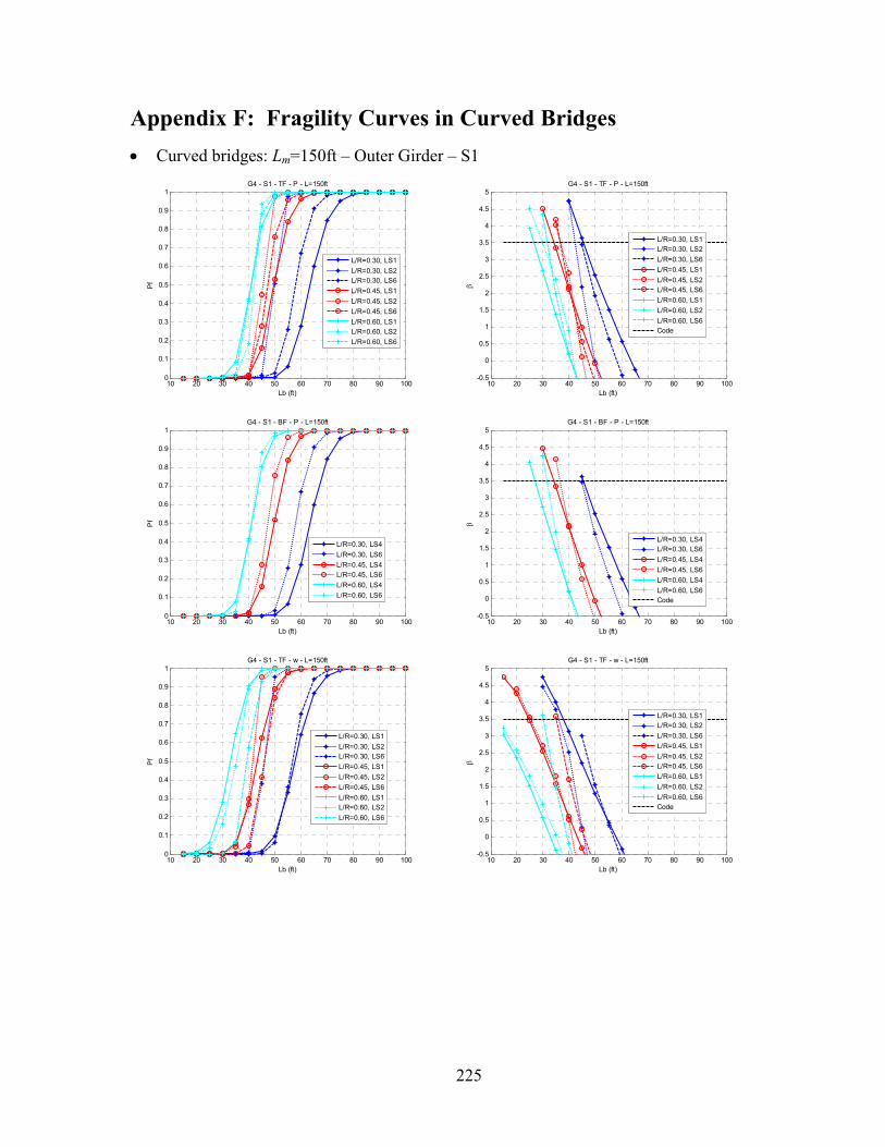
225
Appendix F: Fragility Curves in Curved Bridges • Curved bridges: Lm=150ft – Outer Girder – S1
10 20 30 40 50 60 70 80 90 1000
0.1
0.2
0.3
0.4
0.5
0.6
0.7
0.8
0.9
1G4 - S1 - TF - P - L=150ft
Lb (ft)
Pf
L/R=0.30, LS1L/R=0.30, LS2L/R=0.30, LS6L/R=0.45, LS1L/R=0.45, LS2L/R=0.45, LS6L/R=0.60, LS1L/R=0.60, LS2L/R=0.60, LS6
10 20 30 40 50 60 70 80 90 100-0.5
0
0.5
1
1.5
2
2.5
3
3.5
4
4.5
5G4 - S1 - TF - P - L=150ft
Lb (ft)
β
L/R=0.30, LS1L/R=0.30, LS2L/R=0.30, LS6L/R=0.45, LS1L/R=0.45, LS2L/R=0.45, LS6L/R=0.60, LS1L/R=0.60, LS2L/R=0.60, LS6Code
10 20 30 40 50 60 70 80 90 1000
0.1
0.2
0.3
0.4
0.5
0.6
0.7
0.8
0.9
1G4 - S1 - BF - P - L=150ft
Lb (ft)
Pf
L/R=0.30, LS4L/R=0.30, LS6L/R=0.45, LS4L/R=0.45, LS6L/R=0.60, LS4L/R=0.60, LS6
10 20 30 40 50 60 70 80 90 100-0.5
0
0.5
1
1.5
2
2.5
3
3.5
4
4.5
5G4 - S1 - BF - P - L=150ft
Lb (ft)
β
L/R=0.30, LS4L/R=0.30, LS6L/R=0.45, LS4L/R=0.45, LS6L/R=0.60, LS4L/R=0.60, LS6Code
10 20 30 40 50 60 70 80 90 1000
0.1
0.2
0.3
0.4
0.5
0.6
0.7
0.8
0.9
1G4 - S1 - TF - w - L=150ft
Lb (ft)
Pf
L/R=0.30, LS1L/R=0.30, LS2L/R=0.30, LS6L/R=0.45, LS1L/R=0.45, LS2L/R=0.45, LS6L/R=0.60, LS1L/R=0.60, LS2L/R=0.60, LS6
10 20 30 40 50 60 70 80 90 100-0.5
0
0.5
1
1.5
2
2.5
3
3.5
4
4.5
5G4 - S1 - TF - w - L=150ft
Lb (ft)
β
L/R=0.30, LS1L/R=0.30, LS2L/R=0.30, LS6L/R=0.45, LS1L/R=0.45, LS2L/R=0.45, LS6L/R=0.60, LS1L/R=0.60, LS2L/R=0.60, LS6Code

226
10 20 30 40 50 60 70 80 90 1000
0.1
0.2
0.3
0.4
0.5
0.6
0.7
0.8
0.9
1G4 - S1 - BF - w - L=150ft
Lb (ft)
Pf
L/R=0.30, LS4L/R=0.30, LS6L/R=0.45, LS4L/R=0.45, LS6L/R=0.60, LS4L/R=0.60, LS6
10 20 30 40 50 60 70 80 90 100-0.5
0
0.5
1
1.5
2
2.5
3
3.5
4
4.5
5G4 - S1 - BF - w - L=150ft
Lb (ft)
β
L/R=0.30, LS4L/R=0.30, LS6L/R=0.45, LS4L/R=0.45, LS6L/R=0.60, LS4L/R=0.60, LS6Code

227
• Curved bridges: Lm=150ft – Outer Girder – S3
10 20 30 40 50 60 70 80 90 1000
0.1
0.2
0.3
0.4
0.5
0.6
0.7
0.8
0.9
1G4 - S3 - TF - P - L=150ft
Lb (ft)
Pf
L/R=0.30, LS1L/R=0.30, LS2L/R=0.30, LS6L/R=0.45, LS1L/R=0.45, LS2L/R=0.45, LS6L/R=0.60, LS1L/R=0.60, LS2L/R=0.60, LS6
10 20 30 40 50 60 70 80 90 100-0.5
0
0.5
1
1.5
2
2.5
3
3.5
4
4.5
5G4 - S3 - TF - P - L=150ft
Lb (ft)
β
L/R=0.30, LS1L/R=0.30, LS2L/R=0.30, LS6L/R=0.45, LS1L/R=0.45, LS2L/R=0.45, LS6L/R=0.60, LS1L/R=0.60, LS2L/R=0.60, LS6Code
10 20 30 40 50 60 70 80 90 1000
0.1
0.2
0.3
0.4
0.5
0.6
0.7
0.8
0.9
1G4 - S3 - BF - P - L=150ft
Lb (ft)
Pf
L/R=0.30, LS4L/R=0.30, LS6L/R=0.45, LS4L/R=0.45, LS6L/R=0.60, LS4L/R=0.60, LS6
10 20 30 40 50 60 70 80 90 100-0.5
0
0.5
1
1.5
2
2.5
3
3.5
4
4.5
5G4 - S3 - BF - P - L=150ft
Lb (ft)
β
L/R=0.30, LS4L/R=0.30, LS6L/R=0.45, LS4L/R=0.45, LS6L/R=0.60, LS4L/R=0.60, LS6Code
10 20 30 40 50 60 70 80 90 1000
0.1
0.2
0.3
0.4
0.5
0.6
0.7
0.8
0.9
1G4 - S3 - TF - w - L=150ft
Lb (ft)
Pf
L/R=0.30, LS1L/R=0.30, LS2L/R=0.30, LS6L/R=0.45, LS1L/R=0.45, LS2L/R=0.45, LS6L/R=0.60, LS1L/R=0.60, LS2L/R=0.60, LS6
10 20 30 40 50 60 70 80 90 100-0.5
0
0.5
1
1.5
2
2.5
3
3.5
4
4.5
5G4 - S3 - TF - w - L=150ft
Lb (ft)
β
L/R=0.30, LS1L/R=0.30, LS2L/R=0.30, LS6L/R=0.45, LS1L/R=0.45, LS2L/R=0.45, LS6L/R=0.60, LS1L/R=0.60, LS2L/R=0.60, LS6Code

228
10 20 30 40 50 60 70 80 90 1000
0.1
0.2
0.3
0.4
0.5
0.6
0.7
0.8
0.9
1G4 - S3 - BF - w - L=150ft
Lb (ft)
Pf
L/R=0.30, LS4L/R=0.30, LS6L/R=0.45, LS4L/R=0.45, LS6L/R=0.60, LS4L/R=0.60, LS6
10 20 30 40 50 60 70 80 90 100-0.5
0
0.5
1
1.5
2
2.5
3
3.5
4
4.5
5G4 - S3 - BF - w - L=150ft
Lb (ft)
β
L/R=0.30, LS4L/R=0.30, LS6L/R=0.45, LS4L/R=0.45, LS6L/R=0.60, LS4L/R=0.60, LS6Code
• Curved bridges: Lm=150ft – Outer Girder – S2
10 20 30 40 50 60 70 80 90 1000
0.1
0.2
0.3
0.4
0.5
0.6
0.7
0.8
0.9
1G4 - S2 - BF - w - L=150ft
Lb (ft)
Pf
L/R=0.30, LS1L/R=0.30, LS2L/R=0.30, LS6L/R=0.45, LS1L/R=0.45, LS2L/R=0.45, LS6L/R=0.60, LS1L/R=0.60, LS2L/R=0.60, LS6
10 20 30 40 50 60 70 80 90 100-0.5
0
0.5
1
1.5
2
2.5
3
3.5
4
4.5
5G4 - S2 - BF - w - L=150ft
Lb (ft)
β
L/R=0.30, LS1L/R=0.30, LS2L/R=0.30, LS6L/R=0.45, LS1L/R=0.45, LS2L/R=0.45, LS6L/R=0.60, LS1L/R=0.60, LS2L/R=0.60, LS6Code
10 20 30 40 50 60 70 80 90 1000
0.1
0.2
0.3
0.4
0.5
0.6
0.7
0.8
0.9
1G4 - S2 - TF - w - L=150ft
Lb (ft)
Pf
L/R=0.30, LS4L/R=0.30, LS6L/R=0.45, LS4L/R=0.45, LS6L/R=0.60, LS4L/R=0.60, LS6
10 20 30 40 50 60 70 80 90 100-0.5
0
0.5
1
1.5
2
2.5
3
3.5
4
4.5
5G4 - S2 - TF - w - L=150ft
Lb (ft)
β
L/R=0.30, LS4L/R=0.30, LS6L/R=0.45, LS4L/R=0.45, LS6L/R=0.60, LS4L/R=0.60, LS6Code

229
• Curved bridges: Lm=240ft – Outer Girder – S1
10 20 30 40 50 60 70 80 90 1000
0.1
0.2
0.3
0.4
0.5
0.6
0.7
0.8
0.9
1G4 - S1 - TF - P - L=240ft
Lb (ft)
Pf
L/R=0.30, LS1L/R=0.30, LS2L/R=0.30, LS6L/R=0.45, LS1L/R=0.45, LS2L/R=0.45, LS6L/R=0.60, LS1L/R=0.60, LS2L/R=0.60, LS6
10 20 30 40 50 60 70 80 90 100-0.5
0
0.5
1
1.5
2
2.5
3
3.5
4
4.5
5G4 - S1 - TF - P - L=240ft
Lb (ft)
β
L/R=0.30, LS1L/R=0.30, LS2L/R=0.30, LS6L/R=0.45, LS1L/R=0.45, LS2L/R=0.45, LS6L/R=0.60, LS1L/R=0.60, LS2L/R=0.60, LS6Code
10 20 30 40 50 60 70 80 90 1000
0.1
0.2
0.3
0.4
0.5
0.6
0.7
0.8
0.9
1G4 - S1 - BF - P - L=240ft
Lb (ft)
Pf
L/R=0.30, LS4L/R=0.30, LS6L/R=0.45, LS4L/R=0.45, LS6L/R=0.60, LS4L/R=0.60, LS6
10 20 30 40 50 60 70 80 90 100-0.5
0
0.5
1
1.5
2
2.5
3
3.5
4
4.5
5G4 - S1 - BF - P - L=240ft
Lb (ft)
βL/R=0.30, LS4L/R=0.30, LS6L/R=0.45, LS4L/R=0.45, LS6L/R=0.60, LS4L/R=0.60, LS6Code
3
10 20 30 40 50 60 70 80 90 1000
0.1
0.2
0.3
0.4
0.5
0.6
0.7
0.8
0.9
1G4 - S1 - TF - w - L=240ft
Lb (ft)
Pf L/R=0.30, LS1
L/R=0.30, LS2L/R=0.30, LS6L/R=0.45, LS1L/R=0.45, LS2L/R=0.45, LS6L/R=0.60, LS1L/R=0.60, LS2L/R=0.60, LS6
10 20 30 40 50 60 70 80 90 100-0.5
0
0.5
1
1.5
2
2.5
3
3.5
4
4.5
5G4 - S1 - TF - w - L=240ft
Lb (ft)
β
L/R=0.30, LS1L/R=0.30, LS2L/R=0.30, LS6L/R=0.45, LS1L/R=0.45, LS2L/R=0.45, LS6L/R=0.60, LS1L/R=0.60, LS2L/R=0.60, LS6Code

230
10 20 30 40 50 60 70 80 90 1000
0.1
0.2
0.3
0.4
0.5
0.6
0.7
0.8
0.9
1G4 - S1 - BF - w - L=240ft
Lb (ft)
Pf
L/R=0.30, LS4L/R=0.30, LS6L/R=0.45, LS4L/R=0.45, LS6L/R=0.60, LS4L/R=0.60, LS6
10 20 30 40 50 60 70 80 90 100-0.5
0
0.5
1
1.5
2
2.5
3
3.5
4
4.5
5G4 - S1 - BF - w - L=240ft
Lb (ft)
β
L/R=0.30, LS4L/R=0.30, LS6L/R=0.45, LS4L/R=0.45, LS6L/R=0.60, LS4L/R=0.60, LS6Code

231
• Curved bridges: Lm=240ft – Outer Girder – S3
10 20 30 40 50 60 70 80 90 1000
0.1
0.2
0.3
0.4
0.5
0.6
0.7
0.8
0.9
1G4 - S3 - TF - P - L=240ft
Lb (ft)
Pf
L/R=0.30, LS1L/R=0.30, LS2L/R=0.30, LS6L/R=0.45, LS1L/R=0.45, LS2L/R=0.45, LS6L/R=0.60, LS1L/R=0.60, LS2L/R=0.60, LS6
10 20 30 40 50 60 70 80 90 100-0.5
0
0.5
1
1.5
2
2.5
3
3.5
4
4.5
5G4 - S3 - TF - P - L=240ft
Lb (ft)
β
L/R=0.30, LS1L/R=0.30, LS2L/R=0.30, LS6L/R=0.45, LS1L/R=0.45, LS2L/R=0.45, LS6L/R=0.60, LS1L/R=0.60, LS2L/R=0.60, LS6Code
10 20 30 40 50 60 70 80 90 1000
0.1
0.2
0.3
0.4
0.5
0.6
0.7
0.8
0.9
1G4 - S3 - BF - P - L=240ft
Lb (ft)
Pf
L/R=0.30, LS4L/R=0.30, LS6L/R=0.45, LS4L/R=0.45, LS6L/R=0.60, LS4L/R=0.60, LS6
10 20 30 40 50 60 70 80 90 100-0.5
0
0.5
1
1.5
2
2.5
3
3.5
4
4.5
5G4 - S3 - BF - P - L=240ft
Lb (ft)
β
L/R=0.30, LS4L/R=0.30, LS6L/R=0.45, LS4L/R=0.45, LS6L/R=0.60, LS4L/R=0.60, LS6Code
10 20 30 40 50 60 70 80 90 1000
0.1
0.2
0.3
0.4
0.5
0.6
0.7
0.8
0.9
1G4 - S3 - TF - w - L=240ft
Lb (ft)
Pf
L/R=0.30, LS1L/R=0.30, LS2L/R=0.30, LS6L/R=0.45, LS1L/R=0.45, LS2L/R=0.45, LS6L/R=0.60, LS1L/R=0.60, LS2L/R=0.60, LS6
10 20 30 40 50 60 70 80 90 100-0.5
0
0.5
1
1.5
2
2.5
3
3.5
4
4.5
5G4 - S3 - TF - w - L=240ft
Lb (ft)
β
L/R=0.30, LS1L/R=0.30, LS2L/R=0.30, LS6L/R=0.45, LS1L/R=0.45, LS2L/R=0.45, LS6L/R=0.60, LS1L/R=0.60, LS2L/R=0.60, LS6Code

232
10 20 30 40 50 60 70 80 90 1000
0.1
0.2
0.3
0.4
0.5
0.6
0.7
0.8
0.9
1G4 - S3 - BF - w - L=240ft
Lb (ft)
Pf
L/R=0.30, LS4L/R=0.30, LS6L/R=0.45, LS4L/R=0.45, LS6L/R=0.60, LS4L/R=0.60, LS6
10 20 30 40 50 60 70 80 90 100-0.5
0
0.5
1
1.5
2
2.5
3
3.5
4
4.5
5G4 - S3 - BF - w - L=240ft
Lb (ft)
β
L/R=0.30, LS4L/R=0.30, LS6L/R=0.45, LS4L/R=0.45, LS6L/R=0.60, LS4L/R=0.60, LS6Code
• Curved bridges: Lm=240ft – Outer Girder – S2
10 20 30 40 50 60 70 80 90 1000
0.1
0.2
0.3
0.4
0.5
0.6
0.7
0.8
0.9
1G4 - S2 - BF - w - L=240ft
Lb (ft)
Pf
L/R=0.30, LS1L/R=0.30, LS2L/R=0.30, LS6L/R=0.45, LS1L/R=0.45, LS2L/R=0.45, LS6L/R=0.60, LS1L/R=0.60, LS2L/R=0.60, LS6
10 20 30 40 50 60 70 80 90 100-0.5
0
0.5
1
1.5
2
2.5
3
3.5
4
4.5
5G4 - S2 - BF - w - L=240ft
Lb (ft)
βL/R=0.30, LS1L/R=0.30, LS2L/R=0.30, LS6L/R=0.45, LS1L/R=0.45, LS2L/R=0.45, LS6L/R=0.60, LS1L/R=0.60, LS2L/R=0.60, LS6Code
10 20 30 40 50 60 70 80 90 1000
0.1
0.2
0.3
0.4
0.5
0.6
0.7
0.8
0.9
1G4 - S2 - TF - w - L=240ft
Lb (ft)
Pf
L/R=0.30, LS4L/R=0.30, LS6L/R=0.45, LS4L/R=0.45, LS6L/R=0.60, LS4L/R=0.60, LS6
10 20 30 40 50 60 70 80 90 100-0.5
0
0.5
1
1.5
2
2.5
3
3.5
4
4.5
5G4 - S2 - TF - w - L=240ft
Lb (ft)
β
L/R=0.30, LS4L/R=0.30, LS6L/R=0.45, LS4L/R=0.45, LS6L/R=0.60, LS4L/R=0.60, LS6Code

233
• Curved bridges: Lm=300ft – Outer Girder – S1
10 20 30 40 50 60 70 80 90 1000
0.1
0.2
0.3
0.4
0.5
0.6
0.7
0.8
0.9
1G4 - S1 - TF - P - L=300ft
Lb (ft)
Pf
L/R=0.30, LS1L/R=0.30, LS2L/R=0.30, LS6L/R=0.45, LS1L/R=0.45, LS2L/R=0.45, LS6L/R=0.60, LS1L/R=0.60, LS2L/R=0.60, LS6
10 20 30 40 50 60 70 80 90 100-0.5
0
0.5
1
1.5
2
2.5
3
3.5
4
4.5
5G4 - S1 - TF - P - L=300ft
Lb (ft)
β
L/R=0.30, LS1L/R=0.30, LS2L/R=0.30, LS6L/R=0.45, LS1L/R=0.45, LS2L/R=0.45, LS6L/R=0.60, LS1L/R=0.60, LS2L/R=0.60, LS6Code
10 20 30 40 50 60 70 80 90 1000
0.1
0.2
0.3
0.4
0.5
0.6
0.7
0.8
0.9
1G4 - S1 - BF - P - L=300ft
Lb (ft)
Pf
L/R=0.30, LS4L/R=0.30, LS6L/R=0.45, LS4L/R=0.45, LS6L/R=0.60, LS4L/R=0.60, LS6
10 20 30 40 50 60 70 80 90 100-0.5
0
0.5
1
1.5
2
2.5
3
3.5
4
4.5
5G4 - S1 - BF - P - L=300ft
Lb (ft)
β
L/R=0.30, LS4L/R=0.30, LS6L/R=0.45, LS4L/R=0.45, LS6L/R=0.60, LS4L/R=0.60, LS6Code
10 20 30 40 50 60 70 80 90 1000
0.1
0.2
0.3
0.4
0.5
0.6
0.7
0.8
0.9
1G4 - S1 - TF - w - L=300ft
Lb (ft)
Pf L/R=0.30, LS1
L/R=0.30, LS2L/R=0.30, LS6L/R=0.45, LS1L/R=0.45, LS2L/R=0.45, LS6L/R=0.60, LS1L/R=0.60, LS2L/R=0.60, LS6
10 20 30 40 50 60 70 80 90 100-0.5
0
0.5
1
1.5
2
2.5
3
3.5
4
4.5
5G4 - S1 - TF - w - L=300ft
Lb (ft)
β
L/R=0.30, LS1L/R=0.30, LS2L/R=0.30, LS6L/R=0.45, LS1L/R=0.45, LS2L/R=0.45, LS6L/R=0.60, LS1L/R=0.60, LS2L/R=0.60, LS6Code

234
10 20 30 40 50 60 70 80 90 1000
0.1
0.2
0.3
0.4
0.5
0.6
0.7
0.8
0.9
1G4 - S1 - BF - w - L=300ft
Lb (ft)
Pf
L/R=0.30, LS4L/R=0.30, LS6L/R=0.45, LS4L/R=0.45, LS6L/R=0.60, LS4L/R=0.60, LS6
10 20 30 40 50 60 70 80 90 100-0.5
0
0.5
1
1.5
2
2.5
3
3.5
4
4.5
5G4 - S1 - BF - w - L=300ft
Lb (ft)
β
L/R=0.30, LS4L/R=0.30, LS6L/R=0.45, LS4L/R=0.45, LS6L/R=0.60, LS4L/R=0.60, LS6Code

235
• Curved bridges: Lm=300ft – Outer Girder – S3
10 20 30 40 50 60 70 80 90 1000
0.1
0.2
0.3
0.4
0.5
0.6
0.7
0.8
0.9
1G4 - S3 - TF - P - L=300ft
Lb (ft)
Pf
L/R=0.30, LS1L/R=0.30, LS2L/R=0.30, LS6L/R=0.45, LS1L/R=0.45, LS2L/R=0.45, LS6L/R=0.60, LS1L/R=0.60, LS2L/R=0.60, LS6
10 20 30 40 50 60 70 80 90 100-0.5
0
0.5
1
1.5
2
2.5
3
3.5
4
4.5
5G4 - S3 - TF - P - L=300ft
Lb (ft)
β
L/R=0.30, LS1L/R=0.30, LS2L/R=0.30, LS6L/R=0.45, LS1L/R=0.45, LS2L/R=0.45, LS6L/R=0.60, LS1L/R=0.60, LS2L/R=0.60, LS6Code
10 20 30 40 50 60 70 80 90 1000
0.1
0.2
0.3
0.4
0.5
0.6
0.7
0.8
0.9
1G4 - S3 - BF - P - L=300ft
Lb (ft)
Pf
L/R=0.30, LS4L/R=0.30, LS6L/R=0.45, LS4L/R=0.45, LS6L/R=0.60, LS4L/R=0.60, LS6
10 20 30 40 50 60 70 80 90 100-0.5
0
0.5
1
1.5
2
2.5
3
3.5
4
4.5
5G4 - S3 - BF - P - L=300ft
Lb (ft)
β
L/R=0.30, LS4L/R=0.30, LS6L/R=0.45, LS4L/R=0.45, LS6L/R=0.60, LS4L/R=0.60, LS6Code
10 20 30 40 50 60 70 80 90 1000
0.1
0.2
0.3
0.4
0.5
0.6
0.7
0.8
0.9
1G4 - S3 - TF - w - L=300ft
Lb (ft)
Pf
L/R=0.30, LS1L/R=0.30, LS2L/R=0.30, LS6L/R=0.45, LS1L/R=0.45, LS2L/R=0.45, LS6L/R=0.60, LS1L/R=0.60, LS2L/R=0.60, LS6
10 20 30 40 50 60 70 80 90 100-0.5
0
0.5
1
1.5
2
2.5
3
3.5
4
4.5
5G4 - S3 - TF - w - L=300ft
Lb (ft)
β
L/R=0.30, LS1L/R=0.30, LS2L/R=0.30, LS6L/R=0.45, LS1L/R=0.45, LS2L/R=0.45, LS6L/R=0.60, LS1L/R=0.60, LS2L/R=0.60, LS6Code

236
10 20 30 40 50 60 70 80 90 1000
0.1
0.2
0.3
0.4
0.5
0.6
0.7
0.8
0.9
1G4 - S3 - BF - w - L=300ft
Lb (ft)
Pf
L/R=0.30, LS4L/R=0.30, LS6L/R=0.45, LS4L/R=0.45, LS6L/R=0.60, LS4L/R=0.60, LS6
10 20 30 40 50 60 70 80 90 100-0.5
0
0.5
1
1.5
2
2.5
3
3.5
4
4.5
5G4 - S3 - BF - w - L=300ft
Lb (ft)
β
L/R=0.30, LS4L/R=0.30, LS6L/R=0.45, LS4L/R=0.45, LS6L/R=0.60, LS4L/R=0.60, LS6Code
• Curved bridges: Lm=300ft – Outer Girder – S2
10 20 30 40 50 60 70 80 90 1000
0.1
0.2
0.3
0.4
0.5
0.6
0.7
0.8
0.9
1G4 - S2 - BF - w - L=300ft
Lb (ft)
Pf
L/R=0.30, LS1L/R=0.30, LS2L/R=0.30, LS6L/R=0.45, LS1L/R=0.45, LS2L/R=0.45, LS6L/R=0.60, LS1L/R=0.60, LS2L/R=0.60, LS6
10 20 30 40 50 60 70 80 90 100-0.5
0
0.5
1
1.5
2
2.5
3
3.5
4
4.5
5G4 - S2 - BF - w - L=300ft
Lb (ft)
βL/R=0.30, LS1L/R=0.30, LS2L/R=0.30, LS6L/R=0.45, LS1L/R=0.45, LS2L/R=0.45, LS6L/R=0.60, LS1L/R=0.60, LS2L/R=0.60, LS6Code
10 20 30 40 50 60 70 80 90 1000
0.1
0.2
0.3
0.4
0.5
0.6
0.7
0.8
0.9
1G4 - S2 - TF - w - L=300ft
Lb (ft)
Pf
L/R=0.30, LS4L/R=0.30, LS6L/R=0.45, LS4L/R=0.45, LS6L/R=0.60, LS4L/R=0.60, LS6
10 20 30 40 50 60 70 80 90 100-0.5
0
0.5
1
1.5
2
2.5
3
3.5
4
4.5
5G4 - S2 - TF - w - L=300ft
Lb (ft)
β
L/R=0.30, LS4L/R=0.30, LS6L/R=0.45, LS4L/R=0.45, LS6L/R=0.60, LS4L/R=0.60, LS6Code

237
• Curved bridges: Lm=150ft – Inner Girder – S1
10 20 30 40 50 60 70 80 90 1000
0.1
0.2
0.3
0.4
0.5
0.6
0.7
0.8
0.9
1G1 - S1 - TF - P - L=150ft
Lb (ft)
Pf
L/R=0.30, LS1L/R=0.30, LS2L/R=0.30, LS6L/R=0.45, LS1L/R=0.45, LS2L/R=0.45, LS6L/R=0.60, LS1L/R=0.60, LS2L/R=0.60, LS6
10 20 30 40 50 60 70 80 90 100-0.5
0
0.5
1
1.5
2
2.5
3
3.5
4
4.5
5G1 - S1 - TF - P - L=150ft
Lb (ft)
β
L/R=0.30, LS1L/R=0.30, LS2L/R=0.30, LS6L/R=0.45, LS1L/R=0.45, LS2L/R=0.45, LS6L/R=0.60, LS1L/R=0.60, LS2L/R=0.60, LS6Code
10 20 30 40 50 60 70 80 90 1000
0.1
0.2
0.3
0.4
0.5
0.6
0.7
0.8
0.9
1G1 - S1 - BF - P - L=150ft
Lb (ft)
Pf
L/R=0.30, LS4L/R=0.30, LS6L/R=0.45, LS4L/R=0.45, LS6L/R=0.60, LS4L/R=0.60, LS6
10 20 30 40 50 60 70 80 90 100-0.5
0
0.5
1
1.5
2
2.5
3
3.5
4
4.5
5G1 - S1 - BF - P - L=150ft
Lb (ft)
β
L/R=0.30, LS4L/R=0.30, LS6L/R=0.45, LS4L/R=0.45, LS6L/R=0.60, LS4L/R=0.60, LS6Code
10 20 30 40 50 60 70 80 90 1000
0.1
0.2
0.3
0.4
0.5
0.6
0.7
0.8
0.9
1G1 - S1 - TF - w - L=150ft
Lb (ft)
Pf
L/R=0.30, LS1L/R=0.30, LS2L/R=0.30, LS6L/R=0.45, LS1L/R=0.45, LS2L/R=0.45, LS6L/R=0.60, LS1L/R=0.60, LS2L/R=0.60, LS6
10 20 30 40 50 60 70 80 90 100-0.5
0
0.5
1
1.5
2
2.5
3
3.5
4
4.5
5G1 - S1 - TF - w - L=150ft
Lb (ft)
β
L/R=0.30, LS1L/R=0.30, LS2L/R=0.30, LS6L/R=0.45, LS1L/R=0.45, LS2L/R=0.45, LS6L/R=0.60, LS1L/R=0.60, LS2L/R=0.60, LS6Code
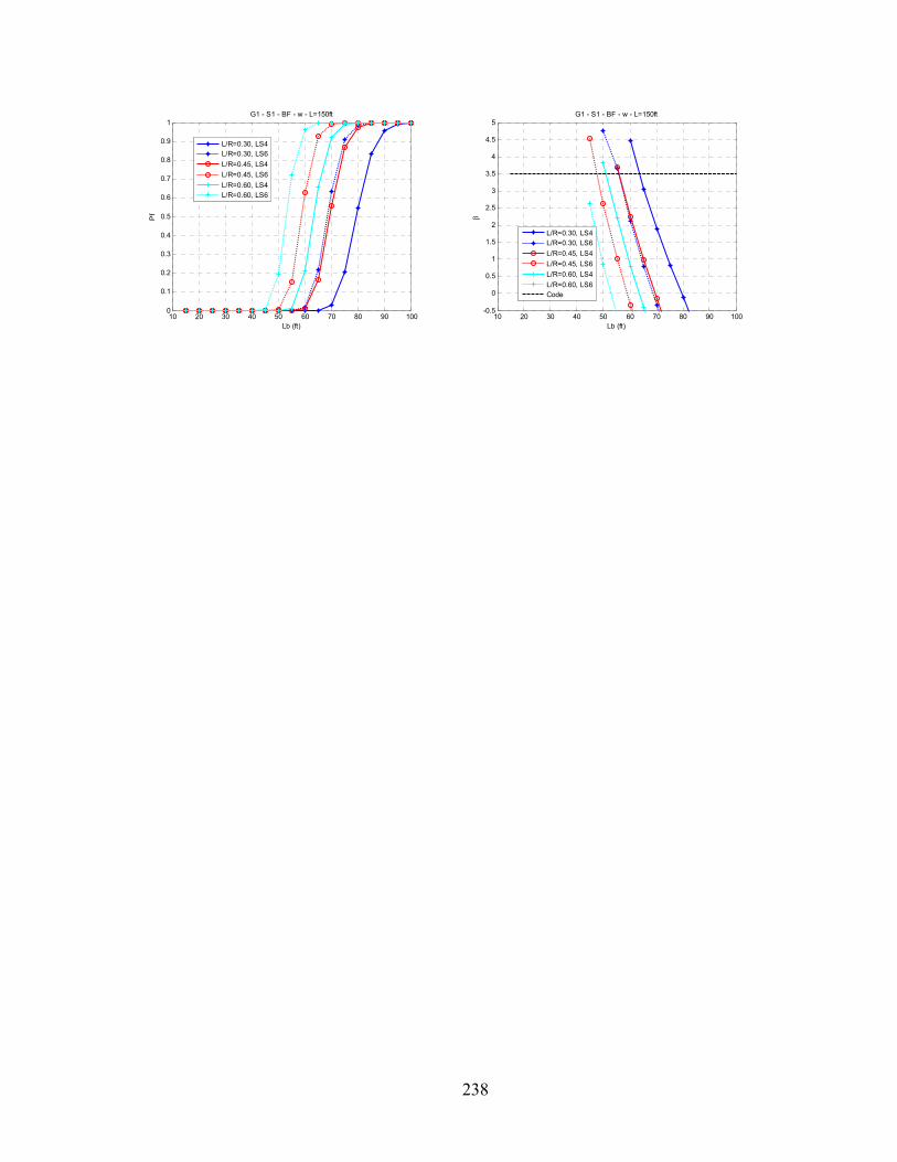
238
10 20 30 40 50 60 70 80 90 1000
0.1
0.2
0.3
0.4
0.5
0.6
0.7
0.8
0.9
1G1 - S1 - BF - w - L=150ft
Lb (ft)
Pf
L/R=0.30, LS4L/R=0.30, LS6L/R=0.45, LS4L/R=0.45, LS6L/R=0.60, LS4L/R=0.60, LS6
10 20 30 40 50 60 70 80 90 100-0.5
0
0.5
1
1.5
2
2.5
3
3.5
4
4.5
5G1 - S1 - BF - w - L=150ft
Lb (ft)
β
L/R=0.30, LS4L/R=0.30, LS6L/R=0.45, LS4L/R=0.45, LS6L/R=0.60, LS4L/R=0.60, LS6Code

239
• Curved bridges: Lm=150ft – Inner Girder – S3
10 20 30 40 50 60 70 80 90 1000
0.1
0.2
0.3
0.4
0.5
0.6
0.7
0.8
0.9
1G1 - S3 - TF - P - L=150ft
Lb (ft)
Pf
L/R=0.30, LS1L/R=0.30, LS2L/R=0.30, LS6L/R=0.45, LS1L/R=0.45, LS2L/R=0.45, LS6L/R=0.60, LS1L/R=0.60, LS2L/R=0.60, LS6
10 20 30 40 50 60 70 80 90 100-0.5
0
0.5
1
1.5
2
2.5
3
3.5
4
4.5
5G1 - S3 - TF - P - L=150ft
Lb (ft)
β
L/R=0.30, LS1L/R=0.30, LS2L/R=0.30, LS6L/R=0.45, LS1L/R=0.45, LS2L/R=0.45, LS6L/R=0.60, LS1L/R=0.60, LS2L/R=0.60, LS6Code
10 20 30 40 50 60 70 80 90 1000
0.1
0.2
0.3
0.4
0.5
0.6
0.7
0.8
0.9
1G1 - S3 - BF - P - L=150ft
Lb (ft)
Pf
L/R=0.30, LS4L/R=0.30, LS6L/R=0.45, LS4L/R=0.45, LS6L/R=0.60, LS4L/R=0.60, LS6
10 20 30 40 50 60 70 80 90 100-0.5
0
0.5
1
1.5
2
2.5
3
3.5
4
4.5
5G1 - S3 - BF - P - L=150ft
Lb (ft)
β
L/R=0.30, LS4L/R=0.30, LS6L/R=0.45, LS4L/R=0.45, LS6L/R=0.60, LS4L/R=0.60, LS6Code
10 20 30 40 50 60 70 80 90 1000
0.1
0.2
0.3
0.4
0.5
0.6
0.7
0.8
0.9
1G1 - S3 - TF - w - L=150ft
Lb (ft)
Pf
L/R=0.30, LS1L/R=0.30, LS2L/R=0.30, LS6L/R=0.45, LS1L/R=0.45, LS2L/R=0.45, LS6L/R=0.60, LS1L/R=0.60, LS2L/R=0.60, LS6
10 20 30 40 50 60 70 80 90 100-0.5
0
0.5
1
1.5
2
2.5
3
3.5
4
4.5
5G1 - S3 - TF - w - L=150ft
Lb (ft)
β
L/R=0.30, LS1L/R=0.30, LS2L/R=0.30, LS6L/R=0.45, LS1L/R=0.45, LS2L/R=0.45, LS6L/R=0.60, LS1L/R=0.60, LS2L/R=0.60, LS6Code

240
10 20 30 40 50 60 70 80 90 1000
0.1
0.2
0.3
0.4
0.5
0.6
0.7
0.8
0.9
1G1 - S3 - BF - w - L=150ft
Lb (ft)
Pf
L/R=0.30, LS4L/R=0.30, LS6L/R=0.45, LS4L/R=0.45, LS6L/R=0.60, LS4L/R=0.60, LS6
10 20 30 40 50 60 70 80 90 100-0.5
0
0.5
1
1.5
2
2.5
3
3.5
4
4.5
5G1 - S3 - BF - w - L=150ft
Lb (ft)
β
L/R=0.30, LS4L/R=0.30, LS6L/R=0.45, LS4L/R=0.45, LS6L/R=0.60, LS4L/R=0.60, LS6Code
• Curved bridges: Lm=150ft – Inner Girder – S2
10 20 30 40 50 60 70 80 90 1000
0.1
0.2
0.3
0.4
0.5
0.6
0.7
0.8
0.9
1G1 - S2 - BF - w - L=150ft
Lb (ft)
Pf
L/R=0.30, LS1L/R=0.30, LS2L/R=0.30, LS6L/R=0.45, LS1L/R=0.45, LS2L/R=0.45, LS6L/R=0.60, LS1L/R=0.60, LS2L/R=0.60, LS6
10 20 30 40 50 60 70 80 90 100-0.5
0
0.5
1
1.5
2
2.5
3
3.5
4
4.5
5G1 - S2 - BF - w - L=150ft
Lb (ft)
β
L/R=0.30, LS1L/R=0.30, LS2L/R=0.30, LS6L/R=0.45, LS1L/R=0.45, LS2L/R=0.45, LS6L/R=0.60, LS1L/R=0.60, LS2L/R=0.60, LS6Code
10 20 30 40 50 60 70 80 90 1000
0.1
0.2
0.3
0.4
0.5
0.6
0.7
0.8
0.9
1G1 - S2 - TF - w - L=150ft
Lb (ft)
Pf
L/R=0.30, LS4L/R=0.30, LS6L/R=0.45, LS4L/R=0.45, LS6L/R=0.60, LS4L/R=0.60, LS6
10 20 30 40 50 60 70 80 90 100-0.5
0
0.5
1
1.5
2
2.5
3
3.5
4
4.5
5G1 - S2 - TF - w - L=150ft
Lb (ft)
β
L/R=0.30, LS4L/R=0.30, LS6L/R=0.45, LS4L/R=0.45, LS6L/R=0.60, LS4L/R=0.60, LS6Code
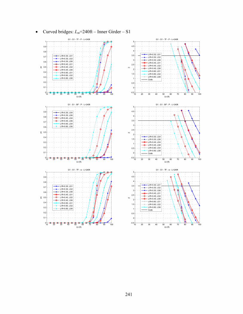
241
• Curved bridges: Lm=240ft – Inner Girder – S1
10 20 30 40 50 60 70 80 90 1000
0.1
0.2
0.3
0.4
0.5
0.6
0.7
0.8
0.9
1G1 - S1 - TF - P - L=240ft
Lb (ft)
Pf
L/R=0.30, LS1L/R=0.30, LS2L/R=0.30, LS6L/R=0.45, LS1L/R=0.45, LS2L/R=0.45, LS6L/R=0.60, LS1L/R=0.60, LS2L/R=0.60, LS6
10 20 30 40 50 60 70 80 90 100-0.5
0
0.5
1
1.5
2
2.5
3
3.5
4
4.5
5G1 - S1 - TF - P - L=240ft
Lb (ft)
β
L/R=0.30, LS1L/R=0.30, LS2L/R=0.30, LS6L/R=0.45, LS1L/R=0.45, LS2L/R=0.45, LS6L/R=0.60, LS1L/R=0.60, LS2L/R=0.60, LS6Code
10 20 30 40 50 60 70 80 90 1000
0.1
0.2
0.3
0.4
0.5
0.6
0.7
0.8
0.9
1G1 - S1 - BF - P - L=240ft
Lb (ft)
Pf
L/R=0.30, LS4L/R=0.30, LS6L/R=0.45, LS4L/R=0.45, LS6L/R=0.60, LS4L/R=0.60, LS6
10 20 30 40 50 60 70 80 90 100-0.5
0
0.5
1
1.5
2
2.5
3
3.5
4
4.5
5G1 - S1 - BF - P - L=240ft
Lb (ft)
β
L/R=0.30, LS4L/R=0.30, LS6L/R=0.45, LS4L/R=0.45, LS6L/R=0.60, LS4L/R=0.60, LS6Code
10 20 30 40 50 60 70 80 90 1000
0.1
0.2
0.3
0.4
0.5
0.6
0.7
0.8
0.9
1G1 - S1 - TF - w - L=240ft
Lb (ft)
Pf
L/R=0.30, LS1L/R=0.30, LS2L/R=0.30, LS6L/R=0.45, LS1L/R=0.45, LS2L/R=0.45, LS6L/R=0.60, LS1L/R=0.60, LS2L/R=0.60, LS6
10 20 30 40 50 60 70 80 90 100-0.5
0
0.5
1
1.5
2
2.5
3
3.5
4
4.5
5G1 - S1 - TF - w - L=240ft
Lb (ft)
β
L/R=0.30, LS1L/R=0.30, LS2L/R=0.30, LS6L/R=0.45, LS1L/R=0.45, LS2L/R=0.45, LS6L/R=0.60, LS1L/R=0.60, LS2L/R=0.60, LS6Code

242
10 20 30 40 50 60 70 80 90 1000
0.1
0.2
0.3
0.4
0.5
0.6
0.7
0.8
0.9
1G1 - S1 - BF - w - L=240ft
Lb (ft)
Pf
L/R=0.30, LS4L/R=0.30, LS6L/R=0.45, LS4L/R=0.45, LS6L/R=0.60, LS4L/R=0.60, LS6
10 20 30 40 50 60 70 80 90 100-0.5
0
0.5
1
1.5
2
2.5
3
3.5
4
4.5
5G1 - S1 - BF - w - L=240ft
Lb (ft)
β
L/R=0.30, LS4L/R=0.30, LS6L/R=0.45, LS4L/R=0.45, LS6L/R=0.60, LS4L/R=0.60, LS6Code

243
• Curved bridges: Lm=240ft – Inner Girder – S3
10 20 30 40 50 60 70 80 90 1000
0.1
0.2
0.3
0.4
0.5
0.6
0.7
0.8
0.9
1G1 - S3 - TF - P - L=240ft
Lb (ft)
Pf
L/R=0.30, LS1L/R=0.30, LS2L/R=0.30, LS6L/R=0.45, LS1L/R=0.45, LS2L/R=0.45, LS6L/R=0.60, LS1L/R=0.60, LS2L/R=0.60, LS6
10 20 30 40 50 60 70 80 90 100-0.5
0
0.5
1
1.5
2
2.5
3
3.5
4
4.5
5G1 - S3 - TF - P - L=240ft
Lb (ft)
β
L/R=0.30, LS1L/R=0.30, LS2L/R=0.30, LS6L/R=0.45, LS1L/R=0.45, LS2L/R=0.45, LS6L/R=0.60, LS1L/R=0.60, LS2L/R=0.60, LS6Code
10 20 30 40 50 60 70 80 90 1000
0.1
0.2
0.3
0.4
0.5
0.6
0.7
0.8
0.9
1G1 - S3 - BF - P - L=240ft
Lb (ft)
Pf
L/R=0.30, LS4L/R=0.30, LS6L/R=0.45, LS4L/R=0.45, LS6L/R=0.60, LS4L/R=0.60, LS6
10 20 30 40 50 60 70 80 90 100-0.5
0
0.5
1
1.5
2
2.5
3
3.5
4
4.5
5G1 - S3 - BF - P - L=240ft
Lb (ft)
β
L/R=0.30, LS4L/R=0.30, LS6L/R=0.45, LS4L/R=0.45, LS6L/R=0.60, LS4L/R=0.60, LS6Code
10 20 30 40 50 60 70 80 90 1000
0.1
0.2
0.3
0.4
0.5
0.6
0.7
0.8
0.9
1G1 - S3 - TF - w - L=240ft
Lb (ft)
Pf
L/R=0.30, LS1L/R=0.30, LS2L/R=0.30, LS6L/R=0.45, LS1L/R=0.45, LS2L/R=0.45, LS6L/R=0.60, LS1L/R=0.60, LS2L/R=0.60, LS6
10 20 30 40 50 60 70 80 90 100-0.5
0
0.5
1
1.5
2
2.5
3
3.5
4
4.5
5G1 - S3 - TF - w - L=240ft
Lb (ft)
β
L/R=0.30, LS1L/R=0.30, LS2L/R=0.30, LS6L/R=0.45, LS1L/R=0.45, LS2L/R=0.45, LS6L/R=0.60, LS1L/R=0.60, LS2L/R=0.60, LS6Code

244
10 20 30 40 50 60 70 80 90 1000
0.1
0.2
0.3
0.4
0.5
0.6
0.7
0.8
0.9
1G1 - S3 - BF - w - L=240ft
Lb (ft)
Pf
L/R=0.30, LS4L/R=0.30, LS6L/R=0.45, LS4L/R=0.45, LS6L/R=0.60, LS4L/R=0.60, LS6
10 20 30 40 50 60 70 80 90 100-0.5
0
0.5
1
1.5
2
2.5
3
3.5
4
4.5
5G1 - S3 - BF - w - L=240ft
Lb (ft)
β
L/R=0.30, LS4L/R=0.30, LS6L/R=0.45, LS4L/R=0.45, LS6L/R=0.60, LS4L/R=0.60, LS6Code
• Curved bridges: Lm=240ft – Inner Girder – S2
10 20 30 40 50 60 70 80 90 1000
0.1
0.2
0.3
0.4
0.5
0.6
0.7
0.8
0.9
1G1 - S2 - BF - w - L=240ft
Lb (ft)
Pf
L/R=0.30, LS1L/R=0.30, LS2L/R=0.30, LS6L/R=0.45, LS1L/R=0.45, LS2L/R=0.45, LS6L/R=0.60, LS1L/R=0.60, LS2L/R=0.60, LS6
10 20 30 40 50 60 70 80 90 100-0.5
0
0.5
1
1.5
2
2.5
3
3.5
4
4.5
5G1 - S2 - BF - w - L=240ft
Lb (ft)
βL/R=0.30, LS1L/R=0.30, LS2L/R=0.30, LS6L/R=0.45, LS1L/R=0.45, LS2L/R=0.45, LS6L/R=0.60, LS1L/R=0.60, LS2L/R=0.60, LS6Code
10 20 30 40 50 60 70 80 90 1000
0.1
0.2
0.3
0.4
0.5
0.6
0.7
0.8
0.9
1G1 - S2 - TF - w - L=240ft
Lb (ft)
Pf
L/R=0.30, LS4L/R=0.30, LS6L/R=0.45, LS4L/R=0.45, LS6L/R=0.60, LS4L/R=0.60, LS6
10 20 30 40 50 60 70 80 90 100-0.5
0
0.5
1
1.5
2
2.5
3
3.5
4
4.5
5G1 - S2 - TF - w - L=240ft
Lb (ft)
β
L/R=0.30, LS4L/R=0.30, LS6L/R=0.45, LS4L/R=0.45, LS6L/R=0.60, LS4L/R=0.60, LS6Code

245
• Curved bridges: Lm=300ft – Inner Girder – S1
10 20 30 40 50 60 70 80 90 1000
0.1
0.2
0.3
0.4
0.5
0.6
0.7
0.8
0.9
1G1 - S1 - TF - P - L=300ft
Lb (ft)
Pf
L/R=0.30, LS1L/R=0.30, LS2L/R=0.30, LS6L/R=0.45, LS1L/R=0.45, LS2L/R=0.45, LS6L/R=0.60, LS1L/R=0.60, LS2L/R=0.60, LS6
10 20 30 40 50 60 70 80 90 100-0.5
0
0.5
1
1.5
2
2.5
3
3.5
4
4.5
5G1 - S1 - TF - P - L=300ft
Lb (ft)
β
L/R=0.30, LS1L/R=0.30, LS2L/R=0.30, LS6L/R=0.45, LS1L/R=0.45, LS2L/R=0.45, LS6L/R=0.60, LS1L/R=0.60, LS2L/R=0.60, LS6Code
10 20 30 40 50 60 70 80 90 1000
0.1
0.2
0.3
0.4
0.5
0.6
0.7
0.8
0.9
1G1 - S1 - TF - w - L=300ft
Lb (ft)
Pf
L/R=0.30, LS1L/R=0.30, LS2L/R=0.30, LS6L/R=0.45, LS1L/R=0.45, LS2L/R=0.45, LS6L/R=0.60, LS1L/R=0.60, LS2L/R=0.60, LS6
10 20 30 40 50 60 70 80 90 100-0.5
0
0.5
1
1.5
2
2.5
3
3.5
4
4.5
5G1 - S1 - TF - w - L=300ft
Lb (ft)
β
L/R=0.30, LS1L/R=0.30, LS2L/R=0.30, LS6L/R=0.45, LS1L/R=0.45, LS2L/R=0.45, LS6L/R=0.60, LS1L/R=0.60, LS2L/R=0.60, LS6Code

246
• Curved bridges: Lm=300ft – Inner Girder – S3
10 20 30 40 50 60 70 80 90 1000
0.1
0.2
0.3
0.4
0.5
0.6
0.7
0.8
0.9
1G1 - S3 - TF - P - L=300ft
Lb (ft)
Pf
L/R=0.30, LS1L/R=0.30, LS2L/R=0.30, LS6L/R=0.45, LS1L/R=0.45, LS2L/R=0.45, LS6L/R=0.60, LS1L/R=0.60, LS2L/R=0.60, LS6
10 20 30 40 50 60 70 80 90 100-0.5
0
0.5
1
1.5
2
2.5
3
3.5
4
4.5
5G1 - S3 - TF - P - L=300ft
Lb (ft)
β
L/R=0.30, LS1L/R=0.30, LS2L/R=0.30, LS6L/R=0.45, LS1L/R=0.45, LS2L/R=0.45, LS6L/R=0.60, LS1L/R=0.60, LS2L/R=0.60, LS6Code
10 20 30 40 50 60 70 80 90 1000
0.1
0.2
0.3
0.4
0.5
0.6
0.7
0.8
0.9
1G1 - S3 - TF - w - L=300ft
Lb (ft)
Pf
L/R=0.30, LS1L/R=0.30, LS2L/R=0.30, LS6L/R=0.45, LS1L/R=0.45, LS2L/R=0.45, LS6L/R=0.60, LS1L/R=0.60, LS2L/R=0.60, LS6
10 20 30 40 50 60 70 80 90 100-0.5
0
0.5
1
1.5
2
2.5
3
3.5
4
4.5
5G1 - S3 - TF - w - L=300ft
Lb (ft)
β
L/R=0.30, LS1L/R=0.30, LS2L/R=0.30, LS6L/R=0.45, LS1L/R=0.45, LS2L/R=0.45, LS6L/R=0.60, LS1L/R=0.60, LS2L/R=0.60, LS6Code
10 20 30 40 50 60 70 80 90 1000
0.1
0.2
0.3
0.4
0.5
0.6
0.7
0.8
0.9
1G1 - S3 - BF - w - L=300ft
Lb (ft)
Pf
L/R=0.30, LS4L/R=0.30, LS6L/R=0.45, LS4L/R=0.45, LS6L/R=0.60, LS4L/R=0.60, LS6
10 20 30 40 50 60 70 80 90 100-0.5
0
0.5
1
1.5
2
2.5
3
3.5
4
4.5
5G1 - S3 - BF - w - L=300ft
Lb (ft)
β
L/R=0.30, LS4L/R=0.30, LS6L/R=0.45, LS4L/R=0.45, LS6L/R=0.60, LS4L/R=0.60, LS6Code

247
• Curved bridges: Lm=300ft – Inner Girder – S2
10 20 30 40 50 60 70 80 90 1000
0.1
0.2
0.3
0.4
0.5
0.6
0.7
0.8
0.9
1G1 - S2 - BF - w - L=300ft
Lb (ft)
Pf
L/R=0.30, LS1L/R=0.30, LS2L/R=0.30, LS6L/R=0.45, LS1L/R=0.45, LS2L/R=0.45, LS6L/R=0.60, LS1L/R=0.60, LS2L/R=0.60, LS6
10 20 30 40 50 60 70 80 90 100-0.5
0
0.5
1
1.5
2
2.5
3
3.5
4
4.5
5G1 - S2 - BF - w - L=300ft
Lb (ft)
β
L/R=0.30, LS1L/R=0.30, LS2L/R=0.30, LS6L/R=0.45, LS1L/R=0.45, LS2L/R=0.45, LS6L/R=0.60, LS1L/R=0.60, LS2L/R=0.60, LS6Code

248
Curriculum Vitae
Nohemy Y. Galindez received her Bachelor of Science in Civil Engineering in
2002 and a Master’s degree in 2005, both with emphasis in structures from Universidad
del Valle, Colombia. She worked during her master studies as an adjunct assistant
professor in the Department of Civil Engineering at Universidad del Valle, teaching
courses related to the mechanics of solids and the structural design of buildings. She
joined the School of Civil and Environmental Engineering at West Virginia University in
2006 to pursue a doctoral degree. Her research interests include steel bridge design,
structural reliability, nonlinear finite element analysis and earthquake-resistant design of
buildings.