LESSONS FROM THE TAYLOR ENERGY OIL SPILL: HISTORY, SEASONALITY, AND

NUTRIENT LIMITATION

by

SARAH JOSEPHINE HARRISON

(Under the Direction of Samantha B. Joye)

ABSTRACT

In 2004, Hurricane Ivan destroyed Taylor Energy platform 23051 in the northern Gulf of

Mexico, and oil has leaked from this site into the marine environment since the platform was

destroyed, resulting in the nation’s longest ongoing offshore oil spill. This thesis explores this

site’s history and environmental context using publicly available records and field observations.

Oil slicks observed at this site are longer and more frequently observed in summer months,

coinciding with seasonal wind and riverine discharge patterns. This seasonal nature of the region

is further manifested in the biogeochemistry of surface water from the site, with higher nutrient

concentrations in the summer compared to fall; hydrocarbon oxidation rates suggest both a

seasonally dynamic and persistent community of oil degrading microorganisms in surface water.

Lessons learned from the Taylor Energy site can be applied to future oil spill response efforts in

the Gulf and beyond.

INDEX WORDS: Oil; Biogeochemistry; Taylor Energy; Gulf of Mexico; Season; Surface

Waters; Chemical Dispersant; Inorganic Nutrients

LESSONS FROM THE TAYLOR ENERGY OIL SPILL: HISTORY, SEASONALITY, AND

NUTRIENT LIMITATION

by

SARAH JOSEPHINE HARRISON

A Thesis Submitted to the Graduate Faculty of the University of Georgia in Partial

Fulfillment of the Requirements for the Degree

MASTER OF SCIENCE

ATHENS, GEORGIA

2017

© 2017

Sarah Josephine Harrison

All Rights Reserved

LESSONS FROM THE TAYLOR ENERGY OIL SPILL: HISTORY, SEASONALITY, AND

NUTRIENT LIMITATION

by

SARAH JOSEPHINE HARRISON

Major Professor: Samantha B. Joye

Committee: Patricia M. Medeiros

Mary Ann Moran

Electronic Version Approved

Suzanne Barbour

Dean of the Graduate School

The University of Georgia

December 2017

iv

ACKNOWLEDGMENTS

Many hands helped bring this project over the finish line. I would like to sincerely thank

my advisor, Mandy Joye, and committee, Patricia Medeiros and Mary Ann Moran, for their

support, advice, and encouragement to finish both my thesis and pursue an internship with the

National Oceanic and Atmospheric Administration during my final year of graduate school. I

would especially like to thank Mandy Joye for demonstrating that it is possible to research,

educate about, and advocate for the ocean.

This project would not have been possible without the support of my lab mates, both past

and present; many thanks go out to Mary Kate Rogener, Andy Montgomery, Ryan Sibert,

Guangchao Zhang, Cathrine Sheperd, Hannah Chao, Joy Battles, Sarah Herschede, Jessica

Washington, Samantha Waters, Sairah Malkin, Lindsey Fields, Lisa Nigro, Matt Saxton, and

Kim Hunter. I would also like to thank the science party and crew of Endeavor cruise EN559,

especially Leigha Peterson, Kelsey Rogers, and the Montoya Lab from Georgia Tech, for their

efforts in collecting the 2015 samples from the Taylor Site. Sincere thanks to the MacDonald

Lab at Florida State University for the collection of the 2014 samples.

I would also like the Apalachicola Riverkeeper for connecting me with the Tulane

Environmental Law Clinic and Machelle Hall, who generously provided background documents

detailing the site history of the Taylor Energy oil spill. Science does not unfold on a blank stage,

and thank you sincerely for allowing me to examine this site through a historical and legal lens.

v

No part of me would still be standing were it not for the support of my family and

friends. My parents, Nat and Tammy, have always encouraged me to follow my dreams and

blaze whatever medium I need to make my own way on my own terms, and my sister, Natalie

Harrison, has always lent a listening ear and alternative perspective to my own narrow one.

Funding for this research and support for my graduate education has been generously

provided by the University of Georgia Graduate School, the Gulf of Mexico Research Initiative’s

ECOGIG consortium, and the National Science Foundation’s Graduate Research Fellowship

Program.

This work is dedicated in loving memory of three of the best teachers I ever had: Gale

Petronis, Robert Germany, and Vladimir Samarkin.

vi

TABLE OF CONTENTS

Page

ACKNOWLEDGEMENTS………………………………………………………………….…. iv

LIST OF FIGURES…………………………………………………………………………..… ix

LIST OF TABLES …..………………………………………………………………………..... xv

CHAPTER

1. INTRODUCTION……………………………………………...………….... 1

1.1 Taylor Energy Site History…………………………..……………… 1

1.2 Oil at the Sea Surface ……………………………………………… 7

1.3 Aims, Objectives, and Thesis Overview …………………………… 13

References………..…………………………………………………..… 15

2 HIISTORICAL EXAMINATION OF SEASONAL VARIATION AT THE TAYLOR

ENERGY SITE IN THE NORTHERN GULF OF MEXICO …………………………… . 20

2.1 Introduction………………………………………………………… 20

2.2 Description of the Data ………………………...………………….. 21

2.3 Results …………...………………………………………………… 26

2.4 Synthesizing Oil Slick Observations with Meteorological and

Riverine Observations from the Taylor Energy Site..…………...… 48

References ……………………………………………………………... 53

vii

3 A TALE OF TWO TAYLORS: COMPARISON OF THE TAYLOR ENERGY SITE WITH

TWO SEASONALLY DISTINCT TRANSECTS……………………………………….... 54

3.1 Introduction………………………………………………………… 54

3.2 Methods ………………………………………………………...….. 55

3.3 Results.……………………………………………………………... 65

3.4 Discussion………………………………….………………………. 75

3.5 Conclusion……………………………………………………….… 82

References…………………………………………………………….... 83

4 AVAILABILITY OF DISSOLVED NUTRIENTS AND CHEMICAL DISPERSANT

IMPACTS MICROBIAL COMMUNITES AND POTENTIAL HYDROCARBON

OXIDATION RATES IN SURFACE WATER FROM THE TAYLOR ENERGY

SITE ………………………………………………………………...…………………...… 85

4.1 Introduction……………………….………………………………... 85

4.2 Methods and Materials…………………….……………………..… 87

4.3 Results……………………………...………………………………. 96

4.4 Discussion…………………………….………………………..…. 107

4.5 Conclusion……………………………….……………………..… 111

References……………………………...……………………………... 113

5 LESSONS FROM THE TAYLOR ENERGY SITE…………………………………...… 117

5.1 Take Home Lessons from this Study…………………………...… 117

5.2 Recognizing a Dynamic and Changing Gulf of Mexico………..… 118

References…………………...………………………………………... 121

viii

APPENDIX

1. List of Abbreviations……………………………..………………………………. 123

2. Statistical Analyses………………………..………………………………..…….. 125

3. Equations…………………………...………………………………………...…… 126

ix

LIST OF FIGURES

Figure 1.1: The Taylor Energy site in the northern Gulf of Mexico lies southeast of the

Mississippi River’s bird-foot delta (a) and is the site where Taylor Energy platform

23051 (b) once stood in Mississippi Canyon lease block 20 (MC20), before being

destroyed by an underwater mudslide, triggered by Hurricane Ivan (c). Oil has

leaked from the site since the platform fell in 2004…………………………………2

Figure 1.2 Schematic of the Taylor Energy debris field, before and after Hurricane Ivan toppled

the Taylor Energy platform in September 2004. Adapted from BSEE and TEC

documents; not drawn to scale………………………………………………………3

Figure 1.3. Photos from the days the platform deck (a) and jacket (b) were removed from the

seafloor in 2011. The removal process required several weeks of preparation by

divers to excavate and prepare the submerged debris for lifting prior to removal

from the seafloor. Images from TEC………………………………………………..6

Figure 2.1 NDBC stations in the northern Gulf of Mexico…………………………………...24

Figure 2.2 Reported oil slick length (2.2a) and width (2.2b) at the Taylor Energy site from

2004 to 2016. Each dot represents the reported length or width of a slick attributed

to Taylor Energy Company in the northern Gulf of Mexico………………………26

x

Figure 2.3 Reported oil slick length at the Taylor Energy site from 2008-2016 (a). Dot color

indicates the month the slick was observed at the Taylor Energy site. The black line

is a LOESS curve, a non-parametric locally weighted regression curve. Box plots of

reported slick length at the Taylor Energy site from 2008-2016, binned by month

(b) and by meteorological seasons (c)……………………………………………..28

Figure 2.4 Reported oil slick frequencies were tabulated monthly, with the total number of days

with oil slicks reported divided by the number of days in the month, and plotted

over the same period, June 2008- December 2016 (a). Box plots of slick frequency

by month (b) and by season (c)………………………………………………….…31

Figure 2.5 Taylor Energy Site History from 2004 to 2016. Top panel is the timeline of events

documented to have happened at or near the Taylor Energy site that could

potentially influence the ability of observers to document oil at the Taylor Energy

site. The bottom panel is a plot of the monthly slick frequencies over the site

history……………………………………………………………………………...33

Figure 2.6 Photos from TEC following successful removal of Taylor Energy platform 23051

(a) and platform jacket (b) from the seafloor in July and August 2011. Images from

TEC………………………………………………………………………………...34

Figure 2.7 Slick frequency data excluding summers 2010 and 2011 (a). Box plots of slick

frequency by month (b) and by season (c) with the summers of 2010 and 2011

excluded……………………………………………………………………………35

Figure 2.8 Box plots of observed (a) oil slick lengths by year (a), estimated oil slick areas by

year (b), and reported slick frequencies by year (c) at the Taylor Energy site…….38

xi

Figure 2.9 Wind speed data from BURL1 buoy plotted by day, colored by month, and fitted

with a Loess line (a). Wind speed data binned by month (b) and season (c)………40

Figure 2.10 Atmospheric pressure data from PSTL buoy plotted by day, colored by month, and

fitted with a Loess line (a). Pressure data binned by month (b) and season (c)……42

Figure 2.11 Wind direction data from PSTL buoy plotted by day, colored by month, and fitted

with a Loess line (a). Wind direction binned by month (b) and season (c)………..44

Figure 2.12 Data from USGS 07374000 station plotting riverine discharge of the Mississippi

River at Baton Rouge through time (a). Each dot represents the average daily value

for each variable, colored to represent the month in which that data point was

collected. The black line is a Loess curve, a non-parametric locally weighted

regression curve. Discharge data by month (b) and season (c)……………………46

Figure 2.13 Data from USGS 07374000 station plotting dissolved NOx concentrations of the

Mississippi River at Baton Rouge through time (a). Each dot represents the average

daily value for each variable, colored to represent the month in which that data

point was collected. The black line is a Loess curve, a non-parametric locally

weighted regression curve. NOx data by month (b) and season (c)………………..47

Figure 2.14 Correlogram of all variables from the publicly available record using a Spearman's

Rank Correlation Analysis between each variable………………………………...49

Figure 2.15 Schematic of how oil slicks change across seasons at the Taylor Energy site, with

summer on the left, winter on the right…………………………………………….52

xii

Figure 3.1 Map of (a) the northern Gulf of Mexico, (b) the Taylor Energy site, just 11 miles

southeast of the Bird Foot Delta, a slick progressing from the northeast to

southwest, and (c) locations of the stations along the 2014 and 2015 transects…...56

Figure 3.2 Structures of 14C substrates used to quantify hydrocarbon turnover in surface

waters. [1-14C]-n-hexadecane (a) was used as a model linear alkane, and [1,4,5,8-

14C] naphthalene was used as a model aromatic compound (b)…………………...60

Figure 3.3 Schematic of hydrocarbon oxidation rate method developed by Kleindienst et al.

(2015) and Sibert et al. (2016)……………………………………………………..61

Figure 3.4 Average dissolved nutrient concentrations in surface water for each station……...66

Figure 3.5 GC-FID chromatograms of surface slick samples from each of the stations along

the fall 2014 transect……………………………………………………………….68

Figure 3.6 Potential hexadecane oxidation rates by station, yellow bars are from the 2014

transect, green from the 2015 transect……………………………………………..69

Figure 3.7 Potential naphthalene oxidation rates by station, yellow bars are from the 2014

transect, green from the 2015 transect……………………………………………..71

Figure 3.8 Box plots of the potential hexadecane oxidation rate (a) and potential naphthalene

oxidation rate (b) aggregated by transect…………………………………………..72

Figure 3.9 Rate constants for hexadecane oxidation, plus or minus the standard deviation

among the radiotracer replicates. Bars are colored according to the year the sample

was taken…………………………………………………………………………...73

xiii

Figure 3.10 Rate Constants for naphthalene oxidation, plus or minus the standard deviation

among the radiotracer replicates…………………………………………………...74

Figure 3.11 Correlogram of all rates and geochemical parameters from the in situ sampling

regime of the Taylor Energy site, using a Spearman's rank correlation test……….81

Figure 4.1 Map of the Taylor Energy Site in the northern Gulf of Mexico. Regional overview

from Google Maps (left); satellite image of the site with oil emanating from the

source, demarcated with an X (top right); and a map of surface water sampling

locations (shades of blue) featured in this chapter (bottom right)…………………88

Figure 4.2 Schematic of experimental design (a) and sampling design (b)…………………...89

Figure 4.3 Structures of 14C substrates used to quantify hydrocarbon turnover in surface

waters. [1-14C]-n-hexadecane (a) was used as a model linear alkane, and [1,4,5,8-

14C] naphthalene was used as a model aromatic compound (b)…………………...92

Figure 4.4 Schematic of hydrocarbon oxidation rate method developed by Kleindienst et al.

(2015) and Sibert et al. (2016)……………………………………………………..93

Figure 4.5 Bar plots of the dissolved nitrogen species grouped by treatments and shaded by

station after incubation for 24h with each respective treatment…………………...97

Figure 4.6 Bar plots of ammonium drawdown (a) and total dissolved nitrogen drawdown (b)

grouped by treatments and shaded by sites after incubation for 24h with each

respective treatment………………………………………………………………..97

xiv

Figure 4.7 Bar plots of the dissolved organic carbon (DOC) and dissolved organic nitrogen

(DON) concentrations following 24h incubation with each respective treatment.

Plots are grouped by treatments and shaded by site……………………………….99

Figure 4.8 Bar plots of phosphate (a) and total dissolved phosphate (TDP) species (b) grouped

by treatments and shaded by site…………………………………………………100

Figure 4.9 Bar plots of the phosphate drawdown grouped by treatments and shaded by

site………………………………………………………………………………...100

Figure 4.10 Bar plots of the cell counts (a) and virus like particles (b) grouped by treatments

and shaded by site………………………………………………………………...102

Figure 4.11 Bar plots of the potential hexadecane oxidation grouped by treatments and shaded

by site..………………………………………………………………………….103

Figure 4.12 Bar plots of potential naphthalene oxidation rates grouped by treatments and shaded

by site……………………………………………………………………………..105

Figure 4.13 Structure of naphthalene from above and the side with the sp2 hybrid orbitals in

view……………………………………………………………………………….106

Figure 5.1 Map of oil production platforms and pipelines in the northern Gulf of Mexico;

Taylor Energy platform 23051 is marked as a red triangle, while other production

platforms are marked as green dots and pipelines as green lines………………...119

Figure 5.2 Comparison of annual oil fluxes from various sources in the Gulf of Mexico in

barrels of oil per year……………………………………………………………..121

xv

LIST OF TABLES

Table 2.1 Summary of the Wilcoxon Rank Sum Tests for differences in observed oil slick

length by season……………………………………………………………………40

Table 2.2 Summary of the Wilcoxon Rank sum tests for differences in wind speed by season.

Table 2.3 Summary of the Wilcoxon Rank sum tests for differences in atmospheric pressure

by season for PSTL station………………………………………………………...42

Table 2.4 Summary of the Wilcoxon Rank sum tests for differences in wind direction by

season for PSTL station……………………………………………………………44

Table 2.5 Spearman's Rank Correlation Coefficients (ρ) for slick length data and all other

significant metadata from the site………………………………………………….50

Table 3.1 Coordinates for the 2014 transect and 2015 transects……………………………..56

Table 3.2 Table of DNA concentrations for surface water samples from the two Taylor

Energy transects and the amplicon barcodes assigned to each sample using the

protocol developed by Kozich et al. (2013)………………………………………..64

Table 3.3 Table summarizing extractable hydrocarbons for surface water samples from the

two Taylor Energy transects……………………………………………………….67

Table 4.1 Table of potential rates in Kleindienst et al. (2015) and this study………………108

1

CHAPTER 1

INTRODUCTION

1.1 Taylor Energy Site History

The Taylor Energy site refers to the area in the northern Gulf of Mexico where Taylor Energy

Company (TEC) platform 23051 once stood (Figure 1.1a). The site is 17.7 kilometers southeast

of the Mississippi River’s bird-foot delta at a depth of 150 meters. The fixed, 8-pile structure

(Figure 1.1b) was constructed in 1984, with 28 oil and gas wells extending from the structure

into the seafloor, down to reservoirs as deep as 3.35 km deep.

On September 16, 2004, Hurricane Ivan approached Gulf Shores, Alabama as a strong category

3 storm on the Saffir-Simpson scale (Figure 1.1c). The eye of the storm passed 100 km to the

east of the Taylor Energy site, inundating the platform with extensive wind and wave action. The

storm and subsequent storm surge destabilized the seafloor beneath TEC platform 23051,

resulting in an underwater regional slope failure, e.g. an underwater mudslide. As the 8-pile

platform fell to the seafloor, its legs twisted and bent, and the platform and jacket were carried to

rest 170 m down slope and southeast of its original location. The event buried the deck, jacket,

and tangle of pipelines and 28 wells under 30 m of mud and sediment (MMS, 2004). Many of the

wells were significantly damaged. Some of the wells were permanently plugged during the

2

platform’s destruction and subsequent journey across the seafloor, while nine of the wells

survived and were capable of flow in the immediate aftermath of the platform’s destruction.

Figure 1.1 The Taylor Energy site in the northern Gulf of Mexico lies southeast of the Mississippi River’s

bird-foot delta (a) and is the site where Taylor Energy platform 23051 (b) once stood in Mississippi

Canyon lease block 20 (MC20), before being destroyed by an underwater mudslide, triggered by

Hurricane Ivan (c). Oil has leaked from the site since the platform fell in 2004, as pictured in the grey

box of (a).

Oil was first sighted at the sea surface around the Taylor Energy site and reported to the US

Coast Guard (USCG) the day after the hurricane passed through the region, on September 17,

2004 (NRC; SEQNOS ID: 735409). Oil and gas emanated from the seafloor at three discrete

locations across the ~30,000 m2 debris field: oil Plumes A and B were close to the site of the

partially buried jacket and deck, while gas Plume C emanated from the platform’s original

location (Figure 1.2; FRACE, 2014).

3

Figure 1.2 Schematic of the Taylor Energy debris field, before (left) and after (right) Hurricane Ivan

toppled the Taylor Energy platform in September 2004. Adapted from BSEE and TEC documents; not

drawn to scale.

Per the Oil Pollution Act of 1990 (OPA), TEC, the responsible party, is required to pay for the

cost of responding to, containing, and/or removing any oil discharged, or taking other actions “as

may be necessary to minimize or mitigate damage to the public health or welfare, including, but

not limited to, fish, shellfish, wildlife, and public and private property, shorelines, and beaches”

(OPA, 1990), regardless of intent. In March 2008, nearly four years after the platform fell, TEC

and the Minerals Management Service (MMS) entered into a trust agreement to begin the well

decommissioning process. Shortly thereafter, USCG established a Unified Command (UC)

comprised of the TEC, USCG, and MMS to oversee response efforts at the site. MMS ordered

TEC to plug all wells by June 2008, but TEC failed to meet these demands, claiming that the

technology needed to plug the wells at the site did not yet—and still does not—exist. In this

4

unprecedented type of oil spill, TEC had few options for stopping the flow of oil at the site, and,

much like BP in the aftermath of the 2010 Deepwater Horizon blowout, TEC pursued a variety

of previously untested options for oil well intervention and well containment to stop the flow of

oil and gas. Significant efforts were also made to monitor the site for slicks and sheens from mid-

2008 onward.

Well Intervention

Dredging the site to access the wells was deemed too much of an environmental hazard and

safety risk, and so UC pursued alternative intervention strategies. In August 2008, UC capped

nearby pipelines that had been damaged by the storm. Between March 2009 and March 2011,

TEC plugged and abandoned nine wells (wells 1, 4, 10, 11, 13, 16, 17, 19, and 21), all of which

were capable of flow after the platform collapsed (FRACE, 2014). These efforts eliminated the

source of Plume A and Plume B (FRACE, 2014). Drilling intervention wells for the remaining

seventeen wells was deemed too risky for both environmental and health standpoints, and only

four of the remaining wells were deemed capable of flow (wells 2, 3, 8, and 18). By 2013, UC

concluded that intervention activities had stemmed the flow of the nine wells that were capable

of leaking oil after the platform fell, preventing the release of 13-500 barrels of oil per day, or

2050-79,500 L of oil per day (FRACE, 2014).

Containment

UC also explored the plausibility of subsea containment systems as early as mid-2008 to address

the leaking oil while well intervention operations continued. After a brief design period, three

containment domes were installed on the seafloor on May 23, 2009, one over oil Plume A,

5

another over gas Plume C, and the third over a small gas seep adjacent to Plume C. These

containment systems were designed to sit on the seafloor and shunt any leaking oil into a

containment vessel that could be tapped from the surface, collected, and disposed of properly

onshore. In early 2010, Plume A was eliminated through well intervention activities, yet the

containment dome over Plume A’s site continued to yield oily water. Controversy remained over

whether this oil was from a continued leak or from improper cleaning of the containment dome

collection apparatus between deployments. UC concluded that the persistent oil in the

containment drum was most likely emanating from oil-soaked sediments at the site, but there is

little public data to support or refute this claim.

Clearing the debris field

In early 2010, UC prepared to lift platform debris out from under the sediment and off the

seafloor. This endeavor was completed in the summer of 2011 in several steps, first with the

recovery of the platform deck in early July 2011 (Figure 1.3a), followed by the jacket several

weeks later (Figure 1.3b).

6

Figure 1.3. Photos from the days the platform deck (a) and jacket (b) were removed from the seafloor in

2011. The removal process required several weeks of preparation by divers to excavate and prepare the

submerged debris for lifting prior to removal from the seafloor. Images from TEC.

Site Monitoring

In 2008, as part of the response activities, TEC embarked on an extensive oil slick monitoring

program with twice daily overflights of the site. These oil slick sightings were reported to the

National Response Center (NRC), operated by USCG. The NRC is the designation point of

contact across the U.S. and U.S. territories to report all chemical, radioactive, and/or biological

discharges into the environment, including maritime oil spills. The reported information is

publicly available, and contains information about the size of the oil slick, wind direction, sea

conditions, and information on the party responsible for the spill. From 2004 to 2016, there are

over 2,100 discrete NRC reports from the Taylor Energy site where TEC was the designated

responsible party (NRC).

The Future of the Taylor Energy spill

As of 2014, TEC has spent an estimated $435 million on decommissioning activities at the

Taylor Energy site. Despite all well intervention and containment efforts to stymie the flow of oil

7

and gas from the Taylor Energy site, oil slicks at the site persist to this day, and are visible on

satellite images of the area (Figure 1.1a). TEC officials contend that the ongoing source of oil at

the site is from the oil-soaked sediment at the site, while the natural gas at the site is biogenic in

origin (FRACE, 2014). BSEE officials estimate that the volume of oil leaking from this site

ranges from 1 barrel of oil to 55 barrels of oil per day and that oil will continue to leak from the

site for 100 years (BSEE, 2017).

1.2 Oil at the Sea Surface

The fate of oil in the northern Gulf of Mexico has been intensely studied in the wake of the 2010

Deepwater Horizon oil spill, and yet, questions remain about the fate of oil in the marine

environment. The Taylor Energy site offers investigators the opportunity to understand how oil

moves and is biologically processed through marine waters.

As soon as oil is released into the environment, it undergoes a myriad of processes, collectively

referred to as weathering. These processes ultimately transform its chemical composition and

dictate the oil’s fate in the environment. To determine the fate of oil in the environment and to

better respond to future oil spills, these weathering processes must be further characterized and

constrained.

With a lighter density than water, oil released into the marine environment usually makes its way

to the sea surface, forming oil sheens, slicks, or emulsions of gas, water, and oil commonly

referred to as ‘mousse’. There are weathering processes unique to surface waters and the

euphotic zone, including photo-oxidation, evaporation, and emulsification of oil. The combined

8

forces of biodegradation and photo-oxidation are the principle drivers of oil’s transformation in

the marine environment7, but very little effort has been put forth to constrain these forces or to

set biodegradation into the larger context of the surface water ecosystem, where organic matter

and inorganic nutrients are cycled rapidly by microbial communities (Azam et al. 2007; Pomeroy

et al. 1995).

Composition of oil

Petroleum is formed over millions of years from buried organic material subjected to high

temperatures and pressures beneath the Earth’s surface. This process creates a vastly dynamic

mixture that includes solid, liquid, and gaseous hydrocarbons, collectively referred to as

petroleum, and thousands of discrete compounds. The liquid phase is better known as crude oil

and is comprised of four classes of hydrocarbons: saturates, aromatics, resins, and asphaltenes.

The saturated fraction comprises the largest fraction of crude oil by mass, and includes linear,

branched, and cyclic alkanes. The aromatic fraction includes benzene and its alkylated sister

compounds, toluene, ethylbenzene, and xylene (BTEX), as well as polycyclic aromatic

hydrocarbons (PAHs). Although PAHs comprise only a small fraction of oil by mass, these

compounds remain some of the most well studied within oil, as known notorious persistent

organic pollutants, carcinogens (Guengerich et al. 2000), and some have been found to disrupt

cardiac function in fish (Incardona et al. 2004; Brette et al. 2017). The two remaining fractions,

resins and asphaltenes, are complex mixtures within themselves. Both fractions contain high

molecular weight heteroatomic molecules that have yet to be fully described, but are

distinguished functionally by polarity (Peters et al. 2005). The asphaltene fraction is readily

9

precipitated from crude oil upon the addition of a nonpolar solvent, while the resin fraction

remains in solution.

Elementally, oil is predominantly carbon and hydrogen, but may also contain quantities of sulfur,

oxygen, and nitrogen within organic compounds, particularly in the heteroatomic-rich resin and

asphaltene fractions. Oil is also known to contain trace metals, including iron, nickel, vanadium,

aluminum, sodium, calcium, copper, and uranium (Peters et al. 2005; Spiro et al. 2012).

Weathering of Oil

As stated earlier, it is now accepted that oil’s composition is not static as it moves through the

environment. In the wake of the Deepwater Horizon oil spill much research characterized

weathered oil found in the sub-tropical, marine and coastal environments (Aeppli et al. 2014;

Hall et al. 2013; Aeppli et al. 2012; Kiruri et al. 2013; White et al. 2016). Within the water

column, these weathering processes include degradation by microorganisms, dissolution of the

polar fraction, and sedimentation of insoluble constituents. Once at the surface, oil continues to

evolve, losing volatile species to the atmosphere, aromatic species via photooxidative processes,

and microbial degradation of the oil continues. The oil undergoes a predictable succession, with

the disappearance of short chain alkanes and volatile PAHs within a few days. While whole

compounds disappear, new functional groups emerge, including carboxylic acids, esters, and

ketones and the overall oxygen content of the oil increases (Kiruri et al. 2013; Charrie-Duhaut et

al. 2000).

10

Satellite data of oil emanating from natural seeps in the Gulf of Mexico has revealed that oil

slicks at the sea surface are ephemeral, with a mean residence time of 12 hours and a range of 8-

24 hours (MacDonald et al. 1993). Once spilled oil reaches the shore, however, it can persist for

months (Liu et al. 2012; Mendelssohn et al. 2012; Turner et al. 2014) or decades once buried in

the sediment (Reddy et al. 2002). Herein lies the oil paradox: oil in surface waters is ephemeral,

yet if it arrives onshore, it can persist for a very long time. Understanding the processes and

controls on surface slicks will better illuminate the long-term fate of oil in the marine and coastal

environments.

Biodegradation of Oil

The study of hydrocarbon degrading microorganisms dates to the early twentieth century, in the

infancy of the oil industry and microbiology (Zobell, 1946). Some of the earliest studies of

hydrocarbon degradation were conducted in surface waters. By the latter half of the twentieth

century, researchers began to understand the ecological context of these microbial metabolisms.

Wyndham and Costerton (1982) described adhesion by hydrocarbon degrading bacteria to the

underside of surface slicks, resulting in the formation of transparent extracellular polysaccharides

(TEP). Recent studies have sought to characterize the formation of these TEPs in the Gulf of

Mexico, as TEPs are believed to initiate the formation of marine snow, aggregated matrices of

bacteria, phytoplankton, micro-zooplankton, fecal pellets, and other detritus in the water column,

and may play an important role in the global carbon cycle (Ziervogel et al. 2014; Gutierrez et al.

2013).

11

Controls on hydrocarbon degradation in surface waters remain poorly constrained. Malkin and

coauthors demonstrated the important role dissolved nutrients play in regulating hydrocarbon

degrading microbial communities in surface waters (Malkin et al. in prep). Furthermore, the

percolation of oil from the seafloor at natural seeps may also bring dissolved nutrients up to the

surface from deeper, nutrient rich waters (D’souza et al. 2016). Ziervogel et al. (2014) observed

the disappearance of short chain alkanes (n-C12 to n-C21) characteristic of fresh oil and

enrichment of long chain alkanes (>n-C22) after just four days in the northern Gulf, consistent

with what has been observed previously in slightly cooler temperatures (Dutta et al. 2000). The

rapid and predictable removal of n-alkanes is not surprising considering the recent discovery that

strains of the most abundant cyanobacteria, Prochlorococcus and Synechococcus, intracellularly

produce and store linear alkanes (Lea-Smith et al. 2015). Some have even speculated that there is

a symbiotic relationship between alkanogenic cyanobacteria and hydrocarbon degrading

microorganisms in surface waters, which may serve as a reservoir for hydrocarbon degrading

microorganisms (Valentine and Reddy, 2015).

Photooxidation of Oil

The saturated fraction of oil has long thought to be resistant to photooxidation, while the

aromatic fraction of oil is particularly susceptible to photooxidation, owing to the abundance of

delocalized electrons on either side of planar aromatic compounds (Garrett et al. 1998). The

susceptibility to photooxidation increases with increasing molecular weight and increasing alkyl

substitution (Ehrhardt et al. 1992; King et al. 2014). This process is dramatic and rapid, as

demonstrated by King et al. (2014)’s work that tracked the disappearance of 80-90% of high

molecular weight PAHs after just 12 hours of simulated sunlight. The transformed products of

12

photooxidation can then enter the DOC pool, where they have been found to be acutely toxic to

the common brine shrimp, Artemia (Maki et al. 2001). Gros et al. (2014) demonstrated that

photo-oxidation could enrich an oil in the resin-like compounds and in sulfur-containing

moieties, while decreasing the abundance of nitrogen-containing species.

Synergistic Weathering Processes and the Fate of Oil in the Environment

Environmental sampling in the wake of the Deepwater Horizon oil spill revealed that fate of oil

in the marine environment is complex and multifaceted. Work on sand patties found along Gulf

Coast beaches has revealed novel oxyhydrocarbons formed from synergistic weathering

processes, including the photooxidation of saturated hydrocarbons, a fraction long considered to

be photo-resistant (Hall et al. 2013). Not all oil that made it to shore evolved into this extremely

weathered matrix, as demonstrated by the work of Turner et al. (2014) in the oiled marshes of

southern Louisiana, which found alkanes and PAHs characteristic of fresh oil in marsh sediment.

Furthermore, there is evidence that much of the oil returned to the seafloor through synergistic

weathering processes. Specifically, the biodegradation of oil in surface slicks led to the

accumulation of TEPs, triggering the formation of marine oil snow (MOS), which transported at

a minimum 14% of the oil discharged during the Deepwater Horizon release back to the seafloor

in what has been called the Marine Oil Snow Sedimentation and Flocculent Accumulation

(MOSSFA) event (Daly et al. 2016; Valentine et al. 2014). This underwater snowstorm resulted

in a footprint of petrocarbon and 17-α-21-β-hopane on the seafloor (Chanton et al. 2015;

Valentine et al. 2014). The impact of this oil deposition is poorly understood, but one study

found Macondo oil within a brown flocculent matrix on deep sea corals 11 km southwest of the

13

blown out well (White et al. 2012) and there is evidence a similar deposition occurred in the

wake of other major oil spills, including the 1979 IXTOC spill in the southern Gulf of Mexico

(Vonk et al. 2015). The sedimented petrocarbon on the seafloor may be so weathered that it is no

longer within the analytical window of the parent oil it originated from, as evidenced from the

work of Stout et al. in the years after the Macondo blowout (Stout et al. 2016a; Stout et al.

2016b).

1.3 Aims, Objectives, and Overview

The Taylor Energy site offers a rare opportunity to explore the impact of oil in surface waters

across a dynamic range of biogeochemistry conditions. The first chapter explores the history of

the site through careful examination of the public record of slick sightings at the Taylor Energy

site, as well as the metadata from the surrounding northern Gulf of Mexico region. This chapter

aims to understand the nature oil at the site, as well as understanding potential controls on the

fate of oil in surface waters at the site. The next chapter is a biogeochemical comparison of two

transects conducted at different times of the year. In the fall of 2014 and the summer of 2015,

surface water was collected from four stations approaching the site of the felled platform and

assessed for dissolved nutrients, microbial community composition, and capacity for degrading

petroleum hydrocarbons using a radiotracer technique. This chapter aims to understand the

interseasonal dynamics and controls of hydrocarbon oxidation and community structure in the

surface waters near this on-going oil spill. The final chapter of this thesis is an amendment

experiment conducted with water from the summer 2015 transect. Water was amended with

excess inorganic nutrients (N and P), with Corexit 9500A, a common chemical dispersant, and

with a combination of the two to examine how oil spill mitigation efforts might alter the capacity

14

for the microbial community to degrade petroleum hydrocarbons. The ultimate goal of this

project is to shed light on the dynamics and drivers for microbial degradation of oil in surface

waters, so that we may be able to better understand and respond to oil spills like the Taylor

Energy oil spill.

15

References

Aeppli, C.; Carmichael, C. A; Nelson, R. K.; Lemkau, K. L.; Graham, W. M.; Redmond, M.

C.; Valentine, D. L.; Reddy, C. M. Oil Weathering after the Deepwater Horizon Disaster

Led to the Formation of Oxygenated Residues. Environ. Sci. Technol. 2012, 46 (16),

8799–8807 DOI: 10.1021/es3015138.

Aeppli, C.; Nelson, R. K.; Radovic, J. R.; Carmichael, C. A.; Valentine, D. L.; Reddy, C. M.

Recalcitrance and Degradation of Petroleum Biomarkers upon Abiotic and Biotic

Natural Weathering of Deepwater Horizon Oil. Environ. Sci. Technol. 2014, 48, 6726–

6734.

Azam, F.; Malfatti, F. Microbial Structuring of Marine Ecosystems. Nat. Rev. Microbiol. 2007,

5 (10), 782–791 DOI: 10.1038/nrmicro1798.

Brette, F.; Shiels, H. A.; Galli, G. L. J.; Cros, C.; Incardona, J. P.; Scholz, N. L.; Block, B. A. A

Novel Cardiotoxic Mechanism for a Pervasive Global Pollutant. Sci. Rep. 2017, 7,

41476 DOI: 10.1038/srep41476.

Bureau of Safety and Environmental Enforcement (BSEE) and Bureau of Ocean Energy

Management (BOEM). Incident Archive- Taylor Energy Oil Discharge at MC-20 Site

and Ongoing Response Efforts. Retrieved 5/1/2017 from

Https://www.bsee.gov/newsroom/library/incident- Archive/taylor-Energy-Mississippi-

Canyon/ongoing-Response-Efforts. 2017.

Chanton, J.; Zhao, T.; Rosenheim, B. E.; Joye, S. B.; Bosman, S.; Brunner, C.; Yeager, K. M.;

Diercks, A. R.; Hollander, D. Using Natural Abundance Radiocarbon To Trace the Flux

of Petrocarbon to the Seafloor Following the Deepwater Horizon Oil Spill. Environ. Sci.

Technol. 2015, 49, 847–854 DOI: 10.1021/es5046524.

Charrie-Duhaut, A.; Lemoine, S.; Adam, P.; Connan, J.; Albrecht, P. Abiotic Oxidation of

Petroleum Bitumens under Natural Conditions. Org. Geochem. 2000, 31, 977–1003.

D’souza, N. A.; Subramaniam, A.; Juhl, A. R.; Hafez, M.; Chekalyuk, A.; Phan, S.; Yan, B.;

MacDonald, I. R.; Weber, S. C.; Montoya, J. P. Elevated Surface Chlorophyll

Associated with Natural Oil Seeps in the Gulf of Mexico. Nat. Geosci. 2016, 9

(January), 1–4 DOI: 10.1038/ngeo2631.

Daly, K. L.; Passow, U.; Chanton, J.; Hollander, D. Assessing the Impacts of Oil-Associated

Marine Snow Formation and Sedimentation during and after the Deepwater Horizon Oil

Spill. Anthropocene 2016 DOI: 10.1016/j.ancene.2016.01.006.

Dutta, T. K.; Harayama, S. Fate of Crude Oil by the Combination of Photooxidation and

Biodegradation. Environ. Sci. Technol. 2000, 34, 1500–1505.

16

Ehrhardt, M. G.; Burns, K. A.; Bicego, M. C. Sunlight-Induced Compositional Alterations in

the Seawater-Soluble Fraction of a Crude Oil. Mar. Chem. 1992, 37 (1–2), 53–64 DOI:

10.1016/0304-4203(92)90056-G.

Garrett, R. M.; Pickering, I. J.; Haith, C. E.; Prince, R. C. Photooxidation of Crude Oils.

Environ. Sci. Technol. 1998, 32 (23), 3719–3723 DOI: 10.1021/es980201r.

Gros, J.; Reddy, C. M.; Aeppli, C.; Nelson, R. K.; Carmichael, C. A.; Arey, J. S. Resolving

Biodegradation Patterns of Persistent Saturated Hydrocarbons in Weathered Oil

Samples from the Deepwater Horizon Disaster. Environ. Sci. Technol. 2014, 48, 1628–

1637.

Guengerich, F. P. Metabolism of Chemical Carcinogens. Carcinogenesis 2000, 21 (3), 345–

351.

Gutierrez, T.; Berry, D.; Yang, T.; Mishamandani, S.; McKay, L.; Teske, A.; Aitken, M. D.

Role of Bacterial Exopolysaccharides (EPS) in the Fate of the Oil Released during the

Deepwater Horizon Oil Spill. PLoS One 2013, 8 (6), e67717 DOI:

10.1371/journal.pone.0067717.

Hall, G. J.; Frysinger, G. S.; Aeppli, C.; Carmichael, C. a; Gros, J.; Lemkau, K. L.; Nelson, R.

K.; Reddy, C. M. Oxygenated Weathering Products of Deepwater Horizon Oil Come

from Surprising Precursors. Mar. Pollut. Bull. 2013, 75 (1–2), 140–149 DOI:

10.1016/j.marpolbul.2013.07.048.

Incardona, J. P.; Collier, T. K.; Scholz, N. L. Defects in Cardiac Function Precede

Morphological Abnormalities in Fish Embryos Exposed to Polycyclic Aromatic

Hydrocarbons. Toxicol. Appl. Pharmacol. 2004, 196 (2), 191–205 DOI:

10.1016/j.taap.2003.11.026.

King, S. M.; Leaf, P. a; Olson, A. C.; Ray, P. Z.; Tarr, M. a. Photolytic and Photocatalytic

Degradation of Surface Oil from the Deepwater Horizon Spill. Chemosphere 2014, 95

(2014), 415–422 DOI: 10.1016/j.chemosphere.2013.09.060.

Kiruri, L. W.; Dellinger, B.; Lomnicki, S. M. Tar Balls from Deep Water Horizon Oil Spill -

Environmentally Persistent Free Radicals (EPFR) Formation During Crude Weathering.

Environ. Sci. Technol. 2013 DOI: 10.1021/es305157w.

Kleindienst, S.; Seidel, M.; Ziervogel, K.; Grim, S.; Loftis, K.; Harrison, S.; Malkin, S. Y.;

Perkins, M. J.; Field, J.; Sogin, M. L.; Dittmar, T.; Passow, U.; Medeiros, P. M.; Joye, S.

B. Chemical Dispersants Can Suppress the Activity of Natural Oil-Degrading

Microorganisms. Proc. Natl. Acad. Sci. 2015, 112 (48) DOI: 10.1073/pnas.1507380112.

Lea-Smith, D. J.; Biller, S. J.; Davey, M. P.; Cotton, C. a. R.; Perez Sepulveda, B. M.; Turchyn,

A. V.; Scanlan, D. J.; Smith, A. G.; Chisholm, S. W.; Howe, C. J. Contribution of

17

Cyanobacterial Alkane Production to the Ocean Hydrocarbon Cycle. Proc. Natl. Acad.

Sci. 2015, 201507274 DOI: 10.1073/pnas.1507274112.

Liu, Z.; Liu, J.; Zhu, Q.; Wu, W. The Weathering of Oil after the Deepwater Horizon Oil Spill:

Insights from the Chemical Composition of the Oil from the Sea Surface, Salt Marshes

and Sediments. Environ. Res. Lett. 2012, 7 (3), 35302 DOI: 10.1088/1748-

9326/7/3/035302.

MacDonald, I. R.; Guinasso, N. L.; Ackleson, S. G.; Amos, J. F.; Duckworth, R.; Sassen, R.;

Brooks, J. M. Natural Oil Slicks in the Gulf of Mexico Visible from Space. J. Geophys.

Res. 1993, 98 (C9), 16351 DOI: 10.1029/93JC01289.

MacFayden, A.; Wei, E.; Warren, C.; Henry, C.; Watabayashi, G. Utilization of the Northern

Gulf Operational Forecast System to Predict Trajectories of Surface Oil from a

Persistent Source Offshore of the Mississippi River Delta. In 2014 International Oil

Spill Conference; 2014; Vol. 53, pp 1689–1699.

Maki, H.; Sasaki, T.; Harayama, S. Photo-Oxidation of Biodegraded Crude Oil and Toxicity of

the Photo-Oxidized Products. Chemosphere 2001, 44 (5), 1145–1151.

Mendelssohn, I. A.; Andersen, G. L.; Baltz, D. M.; Caffey, R. H.; Carman, K. R.; Fleeger, J.

W.; Joye, S. B.; Lin, Q.; Maltby, E.; Overton, E. B. Oil Impacts on Coastal Wetlands:

Implications for the Mississippi River Delta Ecosystem after the Deepwater Horizon Oil

Spill. Bioscience 2012, 62 (6), 562–574 DOI: 10.1525/bio.2012.62.6.7.

Pomeroy, L. R.; Sheldon, J. E.; Sheldon, W. M.; Peters, F. C. Limits to Growth and Respiration

of Bacterioplankton in the Gulf of Mexico. Mar. Ecol. Prog. Ser. 1995, 117, 259–268.

Reddy, C. M.; Eglinton, T. I.; Hounshell, A.; White, H. K.; Xu, L.; Gaines, R. B.; Frysinger, G.

S. The West Falmouth Oil Spill after Thirty Years: The Persistence of Petroleum

Hydrocarbons in Marsh Sediments. Environ. Sci. Technol. 2002, 36 (22), 4754–4760.

Sibert, R. J.; Harrison, S. J.; Joye, S. B. Protocols for Radiotracer Estimation of Primary

Hydrocarbon Oxidation in Oxygenated Seawater. In Hydrocarbon and Lipid

Microbiology Protocols; McGenity, T. J., Timmis, K. N., Nogales, B., Eds.; Humana

Press, 2016; pp 263–276.

Simister, R. L.; Poutasse, C. M.; Thurston, A. M.; Reeve, J. L.; Baker, M. C.; White, H. K.

Degradation of Oil by Fungi Isolated from Gulf of Mexico Beaches. Mar. Pollut. Bull.

2015, 100 (1), 327–333 DOI: 10.1016/j.marpolbul.2015.08.029.

Spiro, T. G.; Purvis-Roberts, K. L.; Stigliani, W. M. Chemistry of the Environment; University

Science Books, 2012.

18

Stout, S. A.; Payne, J. R. Macondo Oil in Deep-Sea Sediments: Part 1 -- Sub-Sea Weathering of

Oil Deposited on the Seafloor. Mar. Pollut. Bull. 2016, 111 (1–2), 365–380 DOI:

10.1016/j.marpolbul.2016.07.036.

Stout, S. A.; Payne, J. R.; Ricker, R. W.; Baker, G.; Lewis, C. Macondo Oil in Deep-Sea

Sediments: Part 2 -- Distribution and Distinction from Background and Natural Oil

Seeps. Mar. Pollut. Bull. 2016, 111 (1–2), 381–401 DOI:

10.1016/j.marpolbul.2016.07.041.

Taylor Energy Company LLC MC20. FRACE: Final Risk Assessment and Cost Estimate.

Unified Command Summary. March 25-26, 2014.

Taylor Energy Company, LLC. v United States Department of the Interior , No. 09-1029, Mem.

Op. (Washington, D.C. Aug. 31, 2010). 2010.

The Biomarker Guide; Peters, K. E., Walters, C. C., Moldowan, J. M., Eds.; Cambridge

University Press, 2005; Vol. 1.

Turner, R. E.; Overton, E. B.; Meyer, B. M.; Miles, M. S.; McClenachan, G.; Hooper-Bui, L.;

Engel, A. S.; Swenson, E. M.; Lee, J. M.; Milan, C. S.; Gao, H. Distribution and

Recovery Trajectory of Macondo (Mississippi Canyon 252) Oil in Louisiana Coastal

Wetlands. Mar. Pollut. Bull. 2014, 87 (1–2), 57–67 DOI:

10.1016/j.marpolbul.2014.08.011.

United States Department of Interior, Minerals Management Service. MMS Updates Damage

Assessment from Hurricane Ivan. (New Orleans, Oct. 8, 2004). Retrieved 4/27/2017

from https://www.bsee.gov/sites/bsee.gov/files/news/news-item/mms-press-release-

1008a.pdf. 2004.

Valentine, D. L.; Fisher, G. B.; Bagby, S. C.; Nelson, R. K.; Reddy, C. M.; Sylva, S. P.; Woo,

M. a. Fallout Plume of Submerged Oil from Deepwater Horizon. Proc. Natl. Acad. Sci.

2014 DOI: 10.1073/pnas.1414873111.

Valentine, D. L.; Reddy, C. M. Latent Hydrocarbons from Cyanobacteria. Proc. Natl. Acad.

Sci. 2015, 112 (12), 201518485 DOI: 10.1073/pnas.1518485112.

Vonk, S. M.; Hollander, D. J.; Murk, A. T. J. Was the Extreme and Wide-Spread Marine Oil-

Snow Sedimentation and Flocculent Accumulation (MOSSFA) Event during the

Deepwater Horizon Blow-out Unique? Mar. Pollut. Bull. 2015, No. February 2016 DOI:

10.1016/j.marpolbul.2015.08.023.

White, H.; Hsing, P.-Y.; Cho, W.; Shank, T. M.; Cordes, E. E.; Quattrini, A. M.; Nelson, R. K.;

Camilli, R.; Demopoulos, A. W. J.; German, C. R.; Brooks, J. M.; Roberts, H. H.;

Shedd, W.; Reddy, C. M.; Fisher, C. R. Impact of the Deepwater Horizon Oil Spill on a

Deep-Water Coral Community in the Gulf of Mexico. PNAS 2012, 1–6 DOI:

10.1073/pnas.1118029109.

19

Wyndham, R. C.; Costerton, J. W. Bacterionueston Involved in the Oxidation of Hydrocarbons

at the Air-Water Interface. J. Great Lakes Res. 1982, 8 (2), 316–322 DOI:

10.1016/S0380-1330(82)71972-0.

Ziervogel, K.; D’Souza, N.; Sweet, J.; Yan, B.; Passow, U. Natural Oil Slicks Fuel Surface

Water Microbial Activities in the Northern Gulf of Mexico. Front. Microbiol. 2014, 5

(May), 188 DOI: 10.3389/fmicb.2014.00188.

Zobell, C. E. Action of Microorganisms on Hydrocarbons. Bacteriol Rev. 1946, 10 (1–2), 1–49.

20

CHAPTER 2

HISTORICAL EXAMINATION OF SEASONAL VARIATION AT THE TAYLOR

ENERGY SITE IN THE NORTHERN GULF OF MEXICO

2.1 Introduction

In September 2004, Hurricane Ivan destroyed Taylor Energy platform 23051, an 8-pile structure

originally built 17.7 km southeast of the Mississippi River’s bird-foot delta in the northern Gulf

of Mexico. The destruction of the platform and its 28 operational wells has led to pervasive oil

slicks at the site since the platform fell thirteen years ago. Despite the duration of this oil spill,

very little has been done to assess the magnitude of this oil spill or its impact of this oil on

coastal waters in the Gulf of Mexico.

The northern Gulf of Mexico is no stranger to seasonal oscillations. This region experiences

seasonal variations in freshwater inputs from the Mississippi River plume as well as variations in

atmospheric conditions, including wind speed, direction, and rainfall. One prominent example of

how these riverine and meteorological conditions manifest to alter the nature of the water column

is in the annual hypoxic event known as ‘The Dead Zone’ (Rabalais et al. 2002). Nutrient

loading from the Mississippi and Atchafalaya rivers in the spring delivers large amounts of

inorganic nutrients and labile riverine carbon to offshore microbial communities, which rapidly

utilize these inputs in the shallow coastal water column. This nutrient loading in the spring is

followed by periods of stable atmospheric pressure in the summer, which minimizes surface

21

water mixing within the shallow (<100 m) water column. These riverine, atmospheric, and

marine processes converge to deplete the supply of dissolved oxygen in the water column to

hypoxic levels (< 2 mg/L). The 2017 ‘Dead Zone’ was the largest on record, stretching over

22,700 km2, an area the size of the state Connecticut.

This location offers investigators a rare opportunity to explore the impact of oil in surface waters

across a dynamic range of biogeochemical and seasonal conditions. This chapter will collect and

describe all publicly available data on the Taylor Energy site and explore how oil slicks and

other variables change seasonally at this highly dynamic site. The goal is to put these data in

environmental context, describing how atmospheric and riverine influences converge to shape

the fate of oil in the marine environment. This effort will better inform stakeholders and first

responders to future oil spills in the northern Gulf of Mexico.

2.2 Description of the Data

The data included below was collected from a variety of public sources, including the U.S.

Geological Survey (USGS), U.S. Coast Guard (USCG), and the National Oceanographic and

Atmospheric Administration (NOAA).

2.2.1 Oil Slick Observational Data

Oil slick data was collected from the National Response Center and is presently housed by the

U.S. Coast Guard (USCG)'s Maritime Information Exchange (CGMIX). The National Response

Center is a massive database, including every reported chemical spill across the entire U.S. and

22

its territories, including both federal and state waterways. This data repository is comprised of

voluntary reports from individuals after witnessing a chemical spill and/or fire to which might

require emergency response, much like a 9-1-1 emergency line. Reports filed with the NRC can

include precise coordinates of the slick, a quantitative slick description (length, width, area, etc.),

qualitative slick descriptions (e.g. "silvery", "rainbow", etc.), and various levels of

meteorological and maritime observations (wind speed, direction, sea state, etc.), along with

number of injured persons, responsible party, and fire details.

For this study, only oil slick records that included the Taylor Energy Company (TEC) as the

responsible party and located in the region of the felled oil platform in MC20 were included. The

record of observed oil slicks is inconsistent in its coverage, because the information was

collected for regulatory rather than research purposes.

Oil slick dimensions were extracted from the database, converted into kilometers from the

various reporting units, and ordered so that if a difference in length versus width was reported,

length was always greater than the width. For days with multiple filed NRC reports, the average

of all observations were used to describe a slick to not oversample the data. For days in the

record where no slick was reported, value is "N/A" rather than assumed to be zero, as it cannot

be assumed the site was surveyed for oil.

A Shapiro-Wilk normality test concluded that the slick length data does not have a normal

distribution (p-value < 2.2 x 10-16), and so non-parametric modes of analysis were used to

analyze the variance of the slick length data. Kruskal Wallis rank sum tests were used to analyze

for variance of populations, and Wilcoxon rank sum tests were used to test for significant

differences between populations.

23

2.2.2 Buoy Data and Atmospheric Observations

Information on atmospheric conditions was explored using data collected from nearby

observational buoys. The National Data Buoy Center (NDBC) is a unique part of the National

Oceanic and Atmospheric Administration (NOAA)'s National Weather Service (NWS). The

NDBC oversees, designs, and operates a global array of data collecting buoys and coastal

stations, including many stations in the lower Mississippi River and the northern Gulf of Mexico.

Six candidate stations were selected from the NDBC database to gather data from as many

stations surrounding the Taylor Energy site, including other offshore stations (Figure 2.1).

However, there was either no accessible or usable data from the closest offshore stations,

including the KMIS station (operated by the Federal Aviation Administration) or either of the

stations operated by private organizations (Stone Energy platform and CGCL, operated by

Shell). Instead data was curated from the three observation stations in and near the bird-foot

delta.

For this study, buoy data from three NDBC stations were examined: BURL1, PSTL, and PILL1

(Figure 2.1).

1. Station BURL1 is located due Southwest of the Southwest Pass, LA and is owned and

maintained by National Data Buoy Center. BURL1 Coordinates: 28.905 N 89.428 W

(28°54'18" N 89°25'42" W). The buoy located at sea level. Data collected 2009-2016.

2. Station PSTL1 (Buoy ID: 8760922) is located at Pilot's Station East, Southwest Pass, LA,

and is owned and maintained by NOAA's National Ocean Service Water Level

Observation Network. PSTL1 coordinates: 28.932 N 89.407 W (28°55'56" N 89°24'25"

W). The site is located 3.6 m above mean sea level. Data collected 2006-2016.

24

3. Station PILL1 (Buoy ID: 8760721) in Pilottown, LA is owned and maintained by

NOAA's National Ocean Service Water Level Observation Network. PILL1 coordinates:

29.179 N 89.259 W (29°10'45" N 89°15'32" W). The site is located 2.3 m above sea-

level. Data collected 2011-2016.

Figure 2.1 NDBC stations in the northern Gulf of Mexico. Buoys with records featured in this discussion

are in red. Candidate buoys without abundant or accessible data are in pink. The coordinates of the

Taylor Energy site are demarcated by a black diamond.

Buoys featured in this study collected data on wind direction, wind speed, maximum sustained

gust, barometric pressure, air temperature, and water temperature, however, only wind speed,

barometric pressure, and wind direction are discussed in this study. Data was extracted from

these sources, manually aligned, and averaged into daily average values, as many of these

observations were collected at variable intervals, ranging from every five minutes to once per

day.

25

2.2.3 Mississippi River Data

Another important component of this region of the northern Gulf of Mexico is the Mississippi

River, the largest river in North America. The river has seasonal variations with respect to

discharge rates (flow) and nutrient loading. The U.S. Geological Survey (USGS) collects data on

rivers through their National Water Information System program. USGS Station 07374000 is

located at 30°26'44.4", 91°11'29.6"near Baton Rouge, LA and is operated by the USGS Baton

Rouge Field Station, home of the Lower Mississippi—Gulf Water Science Center.

Although this station is 80 km upriver from the Gulf of Mexico, the station is one of the most

well documented in the Lower Mississippi River. Observations from this station include water

temperature, river discharge, river gage height, specific conductivity at 25°C, pH, salinity, stream

level, turbidity, and dissolved NOx- (sum of NO3

- + NO2- in water). For this study, only

temperature, discharge, and NOx- are discussed.

26

2.3 Results

2.3.1 Oil Slick Observations

Figure 2.2 Reported oil slick length (2.2a) and width (2.2b) at the Taylor Energy site from 2004 to 2016.

Each dot represents the reported length or width of a slick attributed to Taylor Energy Company in the

northern Gulf of Mexico. All slick lengths were converted into kilometers from the reported unit(s). The

oil slick surface area values (2.2c) are an estimation that uses the reported slick length and width to

calculate the area of an ellipse as the total surface area of the slick ((Length/2) x (Width/2) x π).

27

The first oil slick sighting attributed to Taylor Energy was recorded on September 14, 2004.

From September 14, 2004 to December 31, 2016, there were 2,083 days out of the 4445 day

record with observed oil slicks in the vicinity of the felled platform and which the CGMIX

database listed TEC as the responsible party (Figure 2.2). This amounts to an average of 0.468

slicks sighted per day over or 1 oil slick every 2.14 days. The reported slick length values range

from 0.27 m to 176 km; observed slick widths vary from 1.2 m to 24 km. To better ascertain the

relative size of these slicks through time, the length and width values were used to calculate the

area of an ellipse, a more conservative estimate than a rectangular surface area (Fig 2.2c). These

estimated areas range from 0.000016700 to 471.78989 km2. Historic profiles of slick width

(Figure 2.2b) and slick area (Figure 2.2c) have the similar profiles, indicating that the upward

trend through time in surface area and overall variance of the surface area data set is driven by

the values of the reported slick widths. There is also a sharp increase in the reported values for

the oil slick width in mid-2014.

2.3.1.1 Observed Oil Slick Length at the Taylor Energy Site

The slick length data can be used to explore intra- and inter-annual variation of oil slicks at the

Taylor Energy Site. Although the record stretches back to September 2004 (Fig 2.1), the

frequency of reports increased steeply in mid-2008, when the USCG established a Unified

Command (UC) to respond to the ongoing oil sightings at the Taylor Energy site (FRACE,

2014). The data for the following section, thus, will only contain data from June 1, 2008-

December 31, 2016. A closer look of the reported slick length reveals that length of the oil slick

sighted varies sinusoidally through time (Figure 2.3a).

28

Figure 2.3 Reported oil slick length at the Taylor Energy site from 2008-2016 (a). Dot color indicates the

month the slick was observed at the Taylor Energy site. The black line is a Loess curve, a non-parametric

locally weighted regression curve. Box plots of reported slick length at the Taylor Energy site from 2008-

2016, binned by month (b) and by meteorological seasons (c). Note the y-scale has been limited to 0-45

km to highlight the seasonal trend, but no data has been omitted from the period.

29

A pair of Kruskal-Wallis rank sum tests found that the population of oil slick length observations

varies significantly between months (Kruskal-Wallis chi-squared = 248.22, df = 11, p-value <

2.2e-16) and between meteorological seasons (Kruskal-Wallis chi-squared = 203.66, df = 3, p-

value < 2.2e-16). Examination between seasonal pairings with a series of Wilcox Rank sum tests

detected significant differences between all seasonal pairings (Table 2.1)

Table 2.1 Summary of the Wilcoxon Rank Sum Tests for differences in observed oil slick length by season.

Spring Summer Fall Winter

Spring n/a

Summer W = 103440, p-value = 1.214e-11 n/a

Fall W = 138360, p-value = 0.002871 W = 103020, p-value < 2.2e-16 n/a

Winter W = 154930, p-value = 1.839e-15 W = 178150, p-value < 2.2e-16 W = 160950, p-value = 5.315e-08 n/a

These data provide substantial evidence that there is a seasonal variation with respect to the

observed oil slick length at the Taylor Energy site in the northern Gulf of Mexico. There are

significantly longer slicks observed in the summer months compared to the spring and fall

months, and the smallest slicks are observed in the winter months. However, the way that the

slick length data was collected is not listed on the CGMIX webpage or documented in any way,

and so the value of these data should be taken with caution and may not reflect a true seasonal

oscillation of slick size at the Taylor Energy site. Additionally, the observed seasonal oscillation

does not necessarily reflect a seasonal oscillation in the rate of oil leaking from the Taylor

Energy site.

30

2.3.1.2 Observation Frequency of Oil Slicks at the Taylor Energy Site

To circumvent the questionable quality of the observational oil slick data, the frequency of oil

slick sightings can be used to examine the seasonal difference in the number of days with an oil

slick(s) reported at the Taylor Energy site. The data included in this section uses the same data as

the previous section, but instead of taking the value of the observation, this section examines the

number of reports per month, reported as Slick Frequency (Equation 2.1).

𝐹𝑠 =[𝑛𝑢𝑚𝑏𝑒𝑟 𝑜𝑓 𝑑𝑎𝑦𝑠 𝑤𝑖𝑡ℎ 𝑟𝑒𝑝𝑜𝑟𝑡𝑒𝑑 𝑠𝑙𝑖𝑐𝑘(𝑠) 𝑖𝑛 𝑡ℎ𝑒 𝑚𝑜𝑛𝑡ℎ]

[𝑡𝑜𝑡𝑎𝑙 𝑛𝑢𝑚𝑏𝑒𝑟 𝑜𝑓 𝑑𝑎𝑦𝑠 𝑖𝑛 𝑡ℎ𝑒 𝑚𝑜𝑛𝑡ℎ]= 𝑛𝑠/𝑛𝑡𝑜𝑡𝑎𝑙

Equation 2.1

The seasonal oscillations are not immediately apparent in this examination of the dataset (Figure

2.4a), nor did statistical tests detect differences in slick frequency by month or by season. The

seasonal trend is somewhat apparent when examining the data by season (Figure 2.4c), and much

less apparent when examining the data by calendar month (Figure 2.4b). This is driven by high

amounts of variance of slick sighting frequency for May, June, July, and August months

compared to all other months.

31

Figure 2.4 Reported oil slick frequencies were tabulated monthly, with the total number of days with oil

slicks reported divided by the number of days in the month, and plotted over the same period, June 2008-

December 2016 (a). Box plots of slick frequency by month (b) and by season (c).

32

To understand the sources of this variance, we must examine the entire record of data (Figure

2.1), which contains three substantial data gaps, which can be better understood if we consider

the complex site history of the Taylor Energy site (Figure 2.5).

The first major gap is from September 2004 to June 2008, when a total of 11 oil slicks were

reported at the site in approximately 3.75 years. This sparse record reflects the fact that the

Unified Command to coordinate the joint industry and federal response effort for the Taylor

Energy oil spill was not established until mid-2008. This process formally began in March 2008,

when the Department of Interior's Minerals Management Service (MMS) entered a trust

agreement with Taylor Energy Company to pay for the response effort (FRACE, 2014).

The second major gap in the data set extends from May 2010 to August 2010. This gap coincides

with the Deepwater Horizon accident, the largest offshore oil spill in U.S. history. The spill

began on April 20, 2010 and lasted until July 15, 2010, when BP successfully plugged the

Macondo well. This spill occurred in Mississippi Canyon Lease Block 252 (MC252), only 62 km

to the southeast of the site of Taylor Energy platform 23051 in Mississippi Canyon Lease Block

20 (MC20). It is likely that many of the oil slicks reported during this time were mistakenly

attributed to the Deepwater Horizon oil spill.

Finally, the third gap in the data set occurred from May to August 2011 and coincided with the

TEC’s efforts to remove debris from the seafloor at the Taylor Energy site. This multi-year effort

culminated with the recovery of the platform deck in early July 2011 and the platform jacket in

August 2011. Images from the Taylor Energy Company reflect that the site was heavily occupied

during these months, thereby obscuring observational efforts during this period (Figure 2.6).

33

Incorporating information about the Taylor Energy site history allows us to better understand

potential sources of the observation variance. Let us look again at the observed slick frequency

data, but this time removing months where slicks could have been misattributed to the

Deepwater Horizon oil spill (May 2010-July 2010) or where the site was not monitored (May-

August 2011).

Figure 2.5 Taylor Energy Site History from 2004 to 2016. Top panel is the timeline of events documented

to have happened at or near the Taylor Energy site that could potentially influence the ability of

observers to document oil at the Taylor Energy site. The bottom panel is a plot of the monthly slick

frequencies over the site history.

34

Figure 2.6 Photos from TEC following successful removal of Taylor Energy platform 23051 (a) and

platform jacket (b) from the seafloor in July and August 2011. Images from TEC.

35

Figure 2.7 Slick frequency data excluding summers 2010 and 2011 (a). Box plots of slick frequency by

month (b) and by season (c) with the summers of 2010 and 2011 excluded. Summer 2010 is excluded

because of the confluence of the Deepwater Horizon oil spill, located 62 km to the southeast of the Taylor

Energy site. Summer 2011 is excluded due to the response activities happening at the Taylor Energy Site.

36

Excluding these time periods (May 2010-July 2010 and May-August 2011) restores some of the

seasonal oscillation observed with the slick length (Figure 2.3). Within this trimmed data set of

slick observations, there was no significant difference in the monthly populations of slick

frequencies (Kruskal-Wallis chi-squared = 15.229, df = 11, p-value = 0.1723). There was,

however a difference in the variance by meteorological season (Kruskal-Wallis chi-squared =

12.376, df = 3, p-value = 0.0062).

Using the Wilcoxon rank sum test to test for differences in the frequency of slick observations by

seasons, no significant differences between summer and spring (W = 174, p-value = 0.1217) or

summer and fall (W = 184, p-value = 0.06544) were detected. However, a significant difference

between summer and winter was detected (W = 379, p-value = 0.003295). The significant

difference between summer and winter months underscores the seasonal oscillation of oil at the

Taylor Energy site. The reason for this seasonal variation could stem from seasonal sampling

bias (more traffic or observations made in the summer) or could reflect seasonal differences

favoring slick formation in summer months compared to other times of the year.

2.3.1.3 Interannual Variation of Oil at the Taylor Energy Site

BOEM and BSEE have classified the persistent leaking oil from the Taylor Energy site as a

‘passive spill’ (BOEM and BSEE, 2016), but many questions remain about how the spill has

changed over its 13-year history. Given the paucity of data collected in the first four years after

the platform was destroyed, we can only examine the record since the site has been monitored in

mid-2008.

A series of Kruskal Wallis rank sum tests examined the slick length and width, by year from

mid-2008 to 2016, and rejected the null hypothesis that these data originated from identical

37

populations (Slick dimensions: Kruskal-Wallis chi-squared = 217.36, df = 8, p-value < 2.2e-16).

Furthermore, this significance is unchanged if we exclude the farthest outlier of recorded slick

lengths (Kruskal-Wallis chi-squared = 216.14, df = 8, p-value < 2.2e-16). Slick frequencies,

excluding summers 2010 and 2011, were also found to originate from non-identical populations

by year (Slick frequency: Kruskal-Wallis chi-squared = 67.824, df = 8, p-value = 1.331e-11).

A Spearman’s Rank Correlation test detected a moderate positive, and statistically significant

relationship between the observed slick length and the year (S= 1073100000, p-value < 2.2e-16,

rho= 0.2957745). A similar correlation is observed between estimated slick area and year (S =

1186400000, p-value < 2.2e-16, rho = 0.2213926), suggesting that the observed oil slicks are

growing larger through time (Figure 2.8 a and b). The slick frequency, however, does not have

the same trend over the entire 8.5-year record examined (S = 142750, p-value = 0.7644, rho= -

0.03132876). Excluding 2016, a clear outlier of the record, however, a Spearman's Rank

correlation coefficient test detected a positive correlation between slick frequency and time (S =

51355, p-value = 3.362e-05, rho = 0.4410686), suggesting that the frequency of observed slicks

is increasing through time, up until 2016 (Figure 2.8c).

38

Figure 2.8 Box plots of observed (a) oil slick lengths by year (a), estimated oil slick areas by year (b),

and reported slick frequencies by year (c) at the Taylor Energy site. Note that the frequency data (c) does

not include summers 2010 and 2011.

39

2.3.2 Seasonal Variations in Meteorological Observations

2.3.2.1 Wind Speed Data

There are substantial seasonal variations with respect to wind speed in the northern Gulf of

Mexico region. The average daily wind speed is highest in the winter months and lowest in the

early summer months. There was strong agreement and significant correlation between all three

stations included in the study, but for simplification, only BURL1 is discussed here. BURL1 had

significant variance by both month and meteorological season.

The sinusoidal oscillation of wind speed at the BURL1 station is even more apparent after

examining the results of the Wilcoxon rank sum tests, which founds significant differences

across all seasons, except for the Spring and Fall (W = 223730, p-value = 0.4683), which have

statistically indistinct wind speeds from one another.

40

Figure 2.9 Wind speed data from BURL1 buoy plotted by day, colored by month, and fitted with a Loess

line (a). Wind speed data binned by month (b) and season (c). No data has been excluded from these

figures.

Table 2.2 Summary of the Wilcoxon Rank sum tests for differences in wind speed by season.

Spring Summer Fall Winter

Spring n/a

Summer W = 264380, p-value < 2.2e-16 n/a

Fall W = 223730, p-value = 0.4683 W = 298730, p-value < 2.2e-16 n/a

Winter W = 146540, p-value < 2.2e-16 W = 66499, p-value < 2.2e-16 W = 168140, p-value < 2.2e-16 n/a

41

2.3.1.2. Atmospheric Pressure Data

Atmospheric pressure also varies significantly within the span of a year, with significantly higher

pressures recorded in the winter compared to summer months. What may be more important for

the Taylor Energy site, however, is the seasonal variance of atmospheric pressure. The variance

of atmospheric pressure is much greater in winter months compared to the summer months,

reflecting greater variation in weather systems are moving through the region. The sinusoidal

oscillation of atmospheric pressure at the PSTL station is even more apparent after examining the

results of the Wilcoxon rank sum test, which found significant differences across all seasons (p-

values <1 e-11), except for the Spring and Fall (p-value = 0.3263), which have statistically

indistinct atmospheric pressures from one another. Similar results were obtained examining the

offshore BURL station, but were excluded for brevity.

42

Figure 2.10 Atmospheric pressure data from PSTL buoy plotted by day, colored by month, and fitted with

a Loess line (a). Pressure data binned by month (b) and season (c). No data has been excluded from these

figures.

Table 2.3 Summary of the Wilcoxon Rank sum tests for differences in atmospheric pressure by season for

PSTL station.

Spring Summer Fall Winter

Spring n/a

Summer W = 266320, p-value = 4.133e-11 n/a

Fall W = 193180, p-value = 0.3263 W = 248910, p-value = 2.2e-14 n/a

Winter W = 126300, p-value < 2.2e-16 W = 93185, p-value < 2.2e-16 W = 120210, p-value < 2.2e-16 n/a

43

2.3.1.3 Wind Direction Data

MacFayden et al. (2014), the only other published study on the Taylor Energy site to date,

observed that oil slicks emanating from the Taylor Energy site range from 0.5-2 km x 10-30 km

in size and vary with respect to the wind conditions. Winds from the south advect oil slicks to the

east from mid-spring to mid-fall, while winds from the north and northeast transport oil slicks to

the west in the fall and winter (MacFayden et al. 2014). Examining the wind direction data from

the three buoy stations confirms the seasonal oscillation of winds, which results in the seasonal

oscillation of where the oil is advected. In the summer months, the wind is predominantly

blowing from the southwest (~225 °), and for the remainder of the year, the wind blows from the

southeast (~ 135 °) (Figure 2.11). This oscillating wind direction reflects that throughout the

year, the oil is likely to be advected in different directions, further underscoring the dynamic

nature of the Taylor Energy site.

44

Figure 2.11 Wind direction data from PSTL buoy plotted by day, colored by month, and fitted with a

Loess line (a). Wind direction binned by month (b) and season (c). No data has been excluded from these

figures.

Table 2.4 Summary of the Wilcoxon Rank sum tests for differences in wind direction by season for PSTL

station.

Spring Summer Fall Winter

Spring n/a

Summer W = 150930, p-value < 2.2 e-16 n/a

Fall W = 147040, p-value < 2.2e-16 W = 105280, p-value < 2.2e-16 n/a

Winter W = 238040, p-value = 1.585e-09 W = 338020, p-value < 2.2e-16 W = 179780, p-value = 0.1787 n/a

45

2.3.2 Mississippi River Observations

In addition to significant oscillations in turbidity, dissolved oxygen, and water temperature (not

shown), there were substantial seasonal oscillations with respect to the rate of riverine discharge

and nitrogen loading at USGS station 07374000 in Baton Rouge, LA. These observations

underscore the highly dynamic nature of the lower Mississippi River. The Taylor Energy site,

located just 18 km offshore, is likely influenced by some of these same drivers, particularly the

discharge and the dissolved nitrogen loading, although there is a multi-day lag between observed

levels at USGS station 07374000 and the Taylor Energy site (Rogener, personal

communication). The discharge rate of the Mississippi River peaks in the late spring, due to the

spring melt upriver, and reaches a minimum in the winter months (Figure 2.12). This discharge

carries large amounts of dissolved organic carbon, sediment, and dissolved nutrients, including

excess nitrogen (Figure 2.13). The seasonal flux of nitrogen from the Mississippi River is

believed to be a primary driver of the annual hypoxic zone in the Gulf of Mexico (Rabalais et al.

2002).

46

Figure 2.12 Data from USGS 07374000 station plotting riverine discharge of the Mississippi River at

Baton Rouge through time (a). Each dot represents the average daily value for each variable, colored to

represent the month in which that data point was collected. The black line is a Loess curve, a non-

parametric locally weighted regression curve. Discharge data by month (b) and season (c). No data has

been excluded from these figures. All data included has been demarcated as 'approved' by the USGS as of

March 2017.

47

Figure 2.13 Data from USGS 07374000 station plotting dissolved NOx concentrations of the Mississippi

River at Baton Rouge through time (a). Each dot represents the average daily value for each variable,

colored to represent the month in which that data point was collected. The black line is a Loess curve, a

non-parametric locally weighted regression curve. NOx data by month (b) and season (c). No data has

been excluded from these figures. All data included has been demarcated as 'approved' by the USGS as of

March 2017.

48

2.4 Synthesizing Oil Slick Observations with the Meteorological and Riverine Observations from

the Taylor Energy Site

The northern Gulf of Mexico is a seasonally dynamic site, and this seasonality extends to the oil

slicks present in surface waters at the Taylor Energy site. From mid-2008-2016, observed oil

slicks were statistically longer and more frequently observed in summer months compared to

other seasons. Meanwhile, winter months have statistically fewer and smaller slicks observed

over the 8.5-year record.

Summer months have statistically lower wind speeds and atmospheric pressures than winter

months, and the wind direction also changes during these summer months. Upriver observations

of the Mississippi River found that the highest rates of discharge occur in the late spring-early

summer months, and nitrogen loading peaks about a month later in mid-summer.

Using a series of Spearman’s Rank Correlation tests, we can synthesize how these

meteorological and riverine observations relate to the oil slick sightings. While these correlations

are not causations, they underscore the site’s dynamic seasonality (Figure 2.14 and Table 2.5).

The hierarchical clustering groups the variables such that the agreement between the three buoy

stations (BURL1, PSTL, and PILL) is clear and statistically significant, with respect to wind

speed, maximum gust velocity, atmospheric pressure, and wind direction.

There is a significant negative relationship between average daily wind speeds and slick length

across all three stations, adding evidence that lower wind speeds correlate with longer oil slicks.

There is also a significant negative relationship between atmospheric pressure and slick length

across all three offshore stations. Previously we established that the lowest atmospheric pressures

49

were observed in the summer, and this negative relationship reflects the coincidence of longer

slicks in summer months with the lower atmospheric pressures. However, we would argue that

the driving force is not the absolute pressure, but the variance in pressure, which is greater in

winter months than in summer months.

Figure 2.14 Correlogram of all variables from the publicly available record using a Spearman's Rank

Correlation Analysis between each variable. The color and shape of each dot on the correlogram is

proportional to the size of the correlation coefficient (ρ), with the color dictating whether the monotonic

relationship described is positive (blue) or negative (red). Variables are clustered hierarchically.

50

Table 2.5 Spearman's Rank Correlation Coefficients (ρ) for slick length data and all other significant

metadata from the site.

Variable Rho p value Category

Elliptical Area (km2) 0.5005121 0.0000000 Slick Observation

Sheen Width (km) 0.1304207 0.0000000 Slick Observation

Square Area (km2) 0.5005121 0.0000000 Slick Observation

Gage Height (m) 0.1457531 0.0000000 Mississippi River

Specific Conductivity -0.0822708 0.0011114 Mississippi River

Discharge (m3s-1) 0.1476230 0.0000000 Mississippi River

NOx (μM) 0.2582545 0.0000000 Mississippi River

Dissolved O2 (μM) -0.3367831 0.0000000 Mississippi River

Water Temperature (°C) 0.2883881 0.0000000 Temperature

Max. Temperature (°C) 0.2812940 0.0000000 Temperature

Min. Temperature (°C) 0.2972207 0.0000000 Temperature

PILL1 Wind Direction 0.1328257 0.0000006 Wind

PSTL Wind Direction 0.1356594 0.0000000 Wind

BURL1 Wind Direction 0.0828905 0.0028774 Wind

PILL1 Maximum Gust -0.0926710 0.0004868 Wind

PSTL Maximum Gust -0.0979151 0.0000420 Wind

BURL1 Maximum Gust -0.1009095 0.0000279 Wind

PSTL Wind Speed -0.1315465 0.0000000 Wind

PILL1 Wind Speed -0.0887776 0.0008354 Wind

BURL1 Wind speed -0.1527836 0.0000000 Wind

Average Wind Speed -0.0880995 0.0000600 Wind

BURL1 Atmospheric Pressure -0.1114665 0.0000594 Atmospheric Pressure

PSTL Atmospheric Pressure -0.1048263 0.0000070 Atmospheric Pressure

PILL1 Atmospheric Pressure -0.1045319 0.0000821 Atmospheric Pressure

Year 0.2957745 0.0000000 Time

51

Additionally, the Spearman's Rank Test shows that there is a very weak, positive relationship

between discharge and observed slick length (ρ = 0.147623, p = 1.661e-11), as well as a weak,

positive relationship between the NOx and observed slick length (ρ = 0.25825, p < 2.2e-16). This

suggests that there are large seasonal inputs of terrestrial material, including DOC, dissolved

nutrients, and perhaps even trace metals, that might be utilized by surface microbial communities

responding to oil in the surface waters of the Taylor Energy site. Further research is required to

determine how rapidly water from the USGS station reaches the Taylor Energy site.

The meteorological conditions near the Taylor Energy site vary throughout the course of the year

with respect to wind speed, atmospheric pressure, and wind direction. These three variables each

can uniquely impact the Taylor Energy site and the fate of oil emanating from the seafloor at the

site of the felled platform. When oil slicks are likely to be more frequent and larger in size, the

Mississippi River can supply high levels of nitrogen, phosphorous, and trace metals that would

be required to degrade the hydrocarbons persisting in surface waters. In the fall and winter, the

changing atmospheric conditions churn up surface water, physically dispersing oil slicks and

dispersing the oil vertically and horizontally in the water column.

52

Figure 2.15 Schematic of how oil slicks change across seasons at the Taylor Energy site, with summer on

the left, winter on the right.

It is important to note that this seasonal variation in oil slick observations does not mean that oil

is leaking seasonally. Instead, what these data show is that the conditions that are favorable for

slick formation are seasonally dependent. In seasons where oil slicks are less frequently sighted

and smaller in size, we can assume that the oil is being mechanically dispersed vertically in the

water column and horizontally at the sea surface. It is interesting to note that in seasons where

nutrients are likely to be limiting (fall and winter) the oil will be more physically dispersed,

while in seasons where nutrients are abundant (spring and summer), oil slicks are more likely to

form. These differences provide the environment with two different routes to address and

respond to oil over the course of a year. These seasonal differences will be explored in the next

chapter.

53

References

Bureau of Ocean Energy Management and Bureau of Safety and Environmental Enforcement

(BOEM and BSEE; DOI). 2016 Update of Occurrence Rates for Offshore Oil Spills.

Report prepared by ABS Consulting Inc. Arlington, VA. July 13, 2016.

Coast Guard Maritime Information Exchange (CGMIX), version 5.4.0. United States Coast

Guard. Accessed 10/17/2016 from https:/cgmix.uscg.mil/

MacFayden, A.; Wei, E.; Warren, C.; Henry, C.; Watabayashi, G. Utilization of the Northern

Gulf Operational Forecast System to Predict Trajectories of Surface Oil from a Persistent

Source Offshore of the Mississippi River Delta. In 2014 International Oil Spill

Conference; 2014; Vol. 53, pp 1689–1699.

National Data Buoy Center (NDBC). Department of Commerce; National Oceanic and

Atmospheric Administration; Center of Excellence in Marine Technology and the

National Weather Service. Stennis Space Center, MS. Accessed 3/17/2017 from

http://www.ndbc.noaa.gov/

National Water Information System (NWIS). Department of the Interior; U.S. Geological

Survey; National Streamflow Information Program and National Water-Quality

Assessment Project. Baton Rouge, LA. Accessed 3/18/2017 from

https://waterdata.usgs.gov/usa/nwis/uv?site_no=07374000

Rabalais, N. N.; Turner, R. E.; Wiseman, W. J. Gulf of Mexico Hypoxia, a.k.a. “The Dead

Zone.” Annu. Rev. Ecol. Syst. 2002, 33, 235–263 DOI:

10.1146/annurev.ecolsys.33.010802.150513.

Taylor Energy Company LLC MC20. FRACE: Final Risk Assessment and Cost Estimate.

Unified Command Summary. March 25-26, 2014.

54

CHAPTER 3

A TALE OF TWO TAYLORS: COMPARISON OF THE TAYLOR ENERGY SITE

WITH TWO SEASONALLY DISTINCT TRANSECTS

3.1 Introduction

In the previous chapter, we established that the northern Gulf of Mexico experiences substantial

seasonal variations with respect to riverine and meteorological inputs, and that these seasonal

oscillations extend to the observed oil slick length and slick frequency at the Taylor Energy site.

These seasonal observations of the macro-environment suggest that there might be seasonal

oscillations at the microscopic level, potentially impacting hydrocarbon degrading dynamics in

surface waters at the Taylor Energy site.

Surface water is of particular interest at the Taylor Energy site, because this is where oil is likely

to accumulate after being released into the water column, and the surface is also where a large

fraction of oil can be transformed via photo-oxidation, evaporation, and biodegradation by

microbial communities. Understanding the long-term fate of oil in marine and coastal

communities requires a thorough understanding of the kinds of transformations possible at the

sea surface.

To understand the seasonal dynamics and to begin understanding the biogeochemical range of

the Taylor Energy site, we conducted two four-point transects of surface water at the Taylor

55

Energy site. The first transect was conducted in October 2014 and the second transect was

conducted in June 2015 (Figure 3.1 and Table 3.1). Surface water was examined along a wide

variety of biogeochemical parameters, including dissolved nutrients, dissolved organic carbon,

microbial community composition, extractable petroleum hydrocarbons, and potential

hydrocarbon oxidation rates. These geochemical parameters were compared within and between

transects to determine how the seasonal oscillations at the macro-scale of the northern Gulf of

Mexico manifest at the Taylor Energy site, and how those seasonal oscillations impact the

surface water’s ability to degrade petroleum derived hydrocarbons.

3.2 Methods

3.2.1 Sampling and Sample Storage

Surface waters were collected in October 2014 from stations A-D (Figure 3.1) by the MacDonald

Lab. Stations A and D had extensive oiling, while stations B and C were in the vicinity of faint,

rainbow sheens (Figure 3.1). Station A was observed to have extensive mousse formation; oil

mousse is defined as an emulsion of oil, water, and gas whipped up by wind and wave action

(Leahy and Colwell, 1990; reference 45 therein). The oil slick at the Taylor Energy site was

described as a rainbow sheen, extending 12.1 km x 0.8 km in size (SEQNOS ID: 1097841; NRC

and CGMIX).

Whole surface water was collected and stored in acid-washed collapsible low-density

polypropylene cube containers (10L). Oil slick samples were collected into combusted glass jars

(120mL) fitted with PTFE lined caps. 1 x 10L whole water sample was taken from each station,

and 4 surface grabs of the oil at the surface were collected from each station. Samples were

placed out of direct sunlight and stored on ice and shipped overnight to Athens, GA, where

56

whole water was subsampled for nutrients, microbial community, and potential hydrocarbon

oxidation rates. Surface grabs were frozen at -20°C for hydrocarbon extraction and analysis via

gas-chromatography mass spectrometry (GC-MS).

Figure 3.1 Map of (a) the northern Gulf of Mexico, (b) the Taylor Energy site, just 11 miles southeast of

the Bird Foot Delta, a slick progressing from the northeast to southwest, and (c) locations of the stations

along the 2014 and 2015 transects. Stations A, B, C, and D were sampled on October 9, 2014 by the

MacDonald Lab, and are depicted in yellow. Stations E, F, G, and H were sampled on June 10, 2015 from

the R/V Endeavor (EN559), are depicted in green. The location of the sunken Taylor Energy platform is

depicted by the black diamond.

Table 3.1 Coordinates for the 2014 transect and 2015 transects.

Fall 2014 Transect Summer 2015 Transect

Station Longitude Latitude Station Longitude Latitude

A 28.91834 -89.0184 E 28.93270 -88.9619

B 28.93243 -89.0093 F 28.92863 -88.9428

C 28.93319 -88.9969 G 28.92365 -88.9270

D 28.93712 -88.9825 H 28.91315 -88.8906

Surface waters were collected in June 2015 from stations E-H (Figure 3.1). According to records

from the National Response Center and CMIX database of chemical spills, the oil slick at the

Taylor Energy site on the day of the summer 2015 transect was 6.9 km x 1.8 km in size and a

57

'silvery' sheen (SEQNOS ID: 1119149). However, by the time R/V Endeavor arrived on station,

no oil sheen was visible or smell detected, as a summer storm had physically dispersed oil from

the surface.

1L aliquots from bucket casts were poured into 1L amber bottles, fitted with PTFE lined caps,

with 3 x 1L samples taken per site (n= 3/station) and sampled for all analytes within 4 hours of

sample collection.

3.2.2 Dissolved Nutrients

Aliquots of whole surface water were filtered (0.2 μm) and preserved at -20°C until analysis of

dissolved organic carbon (DOC), ammonium (NH4+), NOx

- (NO3- + NO2

-), total dissolved

nitrogen (TDN), phosphate (HPO43-), and total dissolved phosphate (TDP). Dissolved organic

nitrogen and total dissolved organic phosphate concentrations were estimated from subtraction of

inorganic species from total dissolved species.

Dissolved organic carbon (DOC) was analyzed by high temperature (680°C) combustion

catalytic oxidation on a total organic carbon analyzer (Shimadzu TOC-Vcph); concentrations

were determined by comparison to a series of potassium hydrogen phthalate standards. Organic

carbon was measured as the non-purgeable organic carbon (NPOC) content with an NDIR

detector, following sparging with phosphoric acid. Total dissolved nitrogen (TDN) was

measured on the same instrument with a TNM-1 module; concentrations were derived from a

glycine standard. Samples were not diluted prior to analysis.

Nitrate plus nitrite (NOx-) concentrations were quantified by a vanadium reduction method using

a vanadium reduction assembly (Antek 745; Braman and Hendrix 1989) coupled with a

chemiluminescent nitric acid detector (Antek 7050; Garside 1982).

58

Nitrite (NO2-) was analyzed in parallel by standard colorimetric assay (Bendschneider and

Robinson, 1952), while ammonium was measured colorimetrically using the standard phenol

hypochlorite method (Solorzano, 1969). Nitrate (NO3-) was determined from the subtraction of

NO2- from NOx

-.

Dissolved phosphate was measured colorimetrically, using the molybdate blue method

(Solorzano and Sharp, 1980). Total dissolved phosphate (TDP) was first precipitated with

magnesium sulfate, and heated with acid to convert organic phosphate into orthophosphate. This

residue was then subjected to colorimetric analysis using the molybdate blue method (Solorzano

and Sharp, 1980). Colorimetric analyses were performed using a Shimadzu UV-1601

spectrophotometer.

3.2.3 Hydrocarbons

Whole unfiltered water was frozen at -20° for analysis of total extractable hydrocarbons using a

method adapted from Kleindeinst et al. (2015) and Kujawinski et al. (2014). Following thawing,

sample volume was determined gravimetrically, and spiked with known quantities of three

deuterated standards (5μg/sample; fluorene-d10, eicosane-d24, and benzo[a]pyrene-d12). Samples

were transferred to combusted 1L glass separation funnels fitted with solvent rinsed PTFE

spigots, and extracted with dichloromethane (2x 250 mL) and hexane (1 x 250 mL). Samples

from stations A and D required additional hexane and dichloromethane washes as there were still

visible sheens of colored oil in the separatory funnel. Organic fractions from each sample were

combined and reduced in volume via rotary evaporation (Buchi Corp.) and solvent exchanged

into hexane. Samples were further reduced to 500 μL under a gentle stream of Ar.

59

Organic extracts were analyzed with a gas chromatography with time of flight mass spectrometry

(GC-TOF-MS; Pegasus 4D GC, LECO, Michigan). 1 μL of each extract was injected with a 1:10

split injection method, and separated on two in-line columns; the primary column was a Rxi-5 Sil

fused silica column (60m x 0.25 mm ID; 0.25μm df; Restek) joined to an Rxi-17 Sil MS fused

silica column (1m x 0.10mm ID x 0.1μm dr; Restek) housed in a secondary GC oven. The GC

oven was held for 3 minutes at 50°C, followed by a 6°C/minute temperature ramp until reaching

320°C, and held for 20 minutes. Time of flight mass spectrometry allowed for the simultaneous

monitoring of ions ranging from 50-575 m/z across the entire method, after a 600 s solvent delay.

Samples from the 2014 transect were also analyzed via gas chromatography coupled with a

flame ionization detector (GC-FID; model 8610C, SRI, California). Briefly, 1 μL of each extract

was manually injected into a GC-FID, equipped with a splitless inlet and separated on a MXT-5

fused silica column (30 m x 0.53mm x 0.5μm; Restek). The GC oven was held at 45°C for 3

minutes, and the oven temperature was increased at 6°C/min to 120°C, and then increased at

10°C/min to 315°C and held at 315°C for 10 min; the FID detector was held at 315°C. Samples

were run alongside a standard curve of n-alkanes (nC7-nC40; heptane- tetracontane), a mixture

of 16 parent PAHs, and a dilution of crude oil as an estimation of total petroleum hydrocarbons

(TPH).

3.2.4 Potential Hydrocarbon Oxidation Rates

Potential hydrocarbon oxidation rates were quantified as the rate of conversion of a radiolabeled

model hydrocarbon into 14CO2 by the microbial community within each bottle (Kleindienst et al.

2015; Sibert et al. 2016). [1-14C]-n-hexadecane (American Radiolabeled Chemicals, Missouri)

was used as the model aliphatic compound, and [1,4,5,8-14C] naphthalene (American

Radiolabeled Chemicals, Missouri) was used as the model aromatic compound (Figure 3.2).

60

Figure 3.2 Structures of 14C substrates used to quantify hydrocarbon turnover in surface waters. [1-14C]-

n-hexadecane (a) was used as a model linear alkane, and [1,4,5,8-14C] naphthalene was used as a model

aromatic compound (b).

Homogenized water from station sample was subsampled into headspace-free, 8mL glass

scintillation vials capped with a PTFE-lined rubber septum (Supelco, Pennsylvania). Each assay

was carried out in triplicate alongside a killed control (2mL of 2M NaOH). 14C-labeled

hydrocarbons were each dissolved in molecular grade ethanol and delivered into each

scintillation vial with a glass syringe (0.5 μCi= 1.35 x 10-5 Bq; 10μL) and inverted gently to

distribute the tracer. Killed controls were injected with tracer and immediately added to the

killing solution (2M NaOH, 2mL) in a 50mL polypropylene conical tube. Incubations were

carried out at room temperature in the dark. Incubations were terminated by transferring the

contents of the scintillation tube into a 50mL polypropylene conical tube prefilled with the

killing solution. Terminated incubations were stored in the basic solution (pH > 10) at room

temperature for up to 3 weeks before acidic distillation of the evolved 14CO2.

61

Figure 3.3 Schematic of hydrocarbon oxidation rate method developed by Kleindienst et al. (2015) and

Sibert et al. (2016).

Evolved 14CO2 was distilled from the terminated incubation in the following method (Figure

3.3). Samples were transferred to 250mL Erlenmeyer flasks capped with rubber stoppers and

clamps and shaken with activated charcoal (1g, Sigma Aldrich) for 6h as a pre-treatment to bind

any unused tracer to the charcoal. Hexadecane oxidation assays were further amended with C18

reverse phase silica gel (250 mg, Supelco) to more effectively bind unused alkane tracer.

Following this pretreatment, the Erlenmeyer flask was fitted with a carbon dioxide trap (1.5 mL,

CarboSorb E®, Perkin Elmer), acidified with concentrated phosphoric acid (5mL), and quickly

stoppered to minimize loss of evolved CO2. Acidified solutions were then shaken overnight to

capture CO2. Radioactivity of the carbon dioxide trap was quantified using a Beckman 6500

liquid scintillation counter, after adding scintillation fluid, (4.5mL, Scintisafe®, Fisher

Scientific) to each trap. Instrumentation blanks were counted after every 10 samples, and total

injected tracer was quantified as the blank corrected average of the 3 injections made into

62

scintillation fluid at the time of the incubation. All values from the scintillation counter were first

blank corrected, and each sample was kill corrected with the value of the kill control for each

sample.

Potential rates were calculated using modifications of the following formula (Equation 3.1). k is

the rate constant, a term derived from the quotient of α, the fraction of radiotracer turned over, by

t, the duration of the incubation. S is the concentration of the substrate.

−𝑑[𝐻𝑦𝑑𝑟𝑜𝑐𝑎𝑟𝑏𝑜𝑛]

𝑑𝑡= 𝑘[𝑆] = 𝛼

𝑡[𝑆] ∗

[𝑅𝑎𝑑𝑖𝑜𝑎𝑐𝑡𝑖𝑣𝑖𝑡𝑦 𝑡𝑢𝑟𝑛𝑒𝑑 𝑜𝑣𝑒𝑟, 𝑑𝑝𝑚]

[𝑅𝑎𝑑𝑖𝑜𝑎𝑐𝑡𝑖𝑣𝑖𝑡𝑦 𝑎𝑑𝑑𝑒𝑑, 𝑑𝑝𝑚]∗ [𝑆]

𝑡

Equation 3.1

Potential Hexadecane Oxidation Rate: [1-14C]-hexadecane + O2 14CO2 + H2O

−𝑑[𝐻𝑒𝑥𝑎𝑑𝑒𝑐𝑎𝑛𝑒]

𝑑𝑡= 𝑘[𝐻𝑒𝑥𝑎𝑑𝑒𝑐𝑎𝑛𝑒] =

𝛼

𝑡∗ [𝐻𝑒𝑥𝑎𝑑𝑒𝑐𝑎𝑛𝑒] =

[ 𝐶14 𝑂2]

[ 𝐶14 − 𝐻𝑒𝑥𝑎𝑑𝑒𝑐𝑎𝑛𝑒 ∗ 𝑡]∗ [𝐻𝑒𝑥𝑎𝑑𝑒𝑐𝑎𝑛𝑒]

Equation 3.2

Potential Naphthalene Oxidation Rate: [1,4,5,8-14C]-naphthalene + O2 14CO2 + H2O

−𝑑[𝑁𝑎𝑝ℎ𝑡ℎ𝑎𝑙𝑒𝑛𝑒]

𝑑𝑡= 𝑘[𝑁𝑎𝑝ℎ𝑡ℎ𝑎𝑙𝑒𝑛𝑒] =

𝛼

𝑡∗ [𝑁𝑎𝑝ℎ𝑡ℎ𝑎𝑙𝑒𝑛𝑒] =

[ 𝐶14 𝑂2]

[ 𝐶14 − 𝑁𝑎𝑝ℎ𝑡ℎ𝑎𝑙𝑒𝑛𝑒 ∗ 𝑡]∗ [𝑁𝑎𝑝ℎ𝑡ℎ𝑎𝑙𝑒𝑛𝑒]

Equation 3.3

Calculated Concentration of the Radiotracer used in the 14C Incubations

[𝐻𝑒𝑥𝑎𝑑𝑒𝑐𝑎𝑛𝑒 𝑡𝑟𝑎𝑐𝑒𝑟] =𝑅𝑎𝑑𝑖𝑜𝑎𝑐𝑡𝑖𝑣𝑖𝑡𝑦 𝑜𝑓 𝑎𝑑𝑑𝑒𝑑 𝑡𝑟𝑎𝑐𝑒𝑟, 𝑑𝑝𝑚

𝑉𝑜𝑙𝑢𝑚𝑒 𝑜𝑓 𝑖𝑛𝑐𝑢𝑏𝑎𝑡𝑖𝑜𝑛 𝑣𝑒𝑠𝑠𝑒𝑙, 𝑚𝐿∗

1 𝑚𝐶𝑖

2.22𝑥109𝑑𝑝𝑚∗

1𝑚𝑚𝑜𝑙

55 𝑚𝐶𝑖

Equation 3.4

[𝑁𝑎𝑝ℎ𝑡ℎ𝑎𝑙𝑒𝑛𝑒 𝑡𝑟𝑎𝑐𝑒𝑟] =𝑅𝑎𝑑𝑖𝑜𝑎𝑐𝑡𝑖𝑣𝑖𝑡𝑦 𝑜𝑓 𝑎𝑑𝑑𝑒𝑑 𝑡𝑟𝑎𝑐𝑒𝑟, 𝑑𝑝𝑚

𝑉𝑜𝑙𝑢𝑚𝑒 𝑜𝑓 𝑖𝑛𝑐𝑢𝑏𝑎𝑡𝑖𝑜𝑛 𝑣𝑒𝑠𝑠𝑒𝑙, 𝑚𝐿∗

1 𝑚𝐶𝑖

2.22𝑥109𝑑𝑝𝑚∗

1𝑚𝑚𝑜𝑙

58 𝑚𝐶𝑖

Equation 3.5

63

The concentration of the added tracer is a function of the incubation vessel dimension (7.5 mL)

and specific activity of the hexadecane and naphthalene tracer, as determined by the

manufacturer (55 Ci/mol and 58 Ci/mol, respectively; Equations 3.2 and 3.3).

Determining which concentration of substrate to use presented a challenge in this study, given

the vastly different concentrations of oil across the two transects. The in situ concentrations of

hexadecane and naphthalene were below the limit of detection via GC-MS for the entire summer

2015 transect and near the limit of detection for stations B and C in the fall 2014 transect (Table

3.3). Additionally, the incubations required a high concentration of radiotracer (1.45 μM for

hexadecane, and 1.10 μM for naphthalene), which were above the solubility limit for both

compounds. Naphthalene fully saturates water at 25°C under standard atmosphere conditions at

0.248 μM (Pearlman et al. 1984), while the measured solubility limit for hexadecane is

considerably lower, at 4.06 nM (Human Metabalome Database and EPIWEB v4.11). The tracer,

then, is a misnomer in this study, as the tracer itself contributes substantially to the concentration

of substrate in the incubation vessel. Given these limitations, the estimations made from these

assays should be considered as potential rates for the given substrate. Additionally, the potential

rates discussed in this study use the sum of the measured substrate in the environment plus the

tracer concentration as the total substrate concentration.

3.2.5 Microbial Community Composition

Microorganisms were filtered onto a Sterivex filter cartridge (0.22μm; Millipore) and flash

frozen in liquid nitrogen. 1L of water was filtered from each station along the fall 2014 transect;

in the summer 2015 transect, 250 mL from each bottle was pooled with other station replicates

for a total of 750 mL water per station (3 bottles/station * 250 mL/bottle= 750 mL).

64

Samples from 2014 were stored at -20C until processing. Samples from 2015 were shipped on

dry ice from Gulfport, MS to Athens, GA and stored at -80C until processing. Sterivex filters

were thawed on ice, the tops removed with sterilized pliers, and the filter cut using sterile

scalpels; the cut filters were immediately processed for DNA extraction using the DNeasy

Powerwater Kit (Qiagen) according to the manufacturer’s directions. Eluted DNA was quantified

using the dsDNA assay kit and a Qubit fluorometer (Invitrogen) (Table 3.2).

Barcoded amplicons of the 16S rRNA were generated using primers amplifying the V4 region

and the AccuPrime Pfx SuperMix kit (Invitrogen) with methods previously described (Kozich

et al. 2013; Table 3.2). Samples were sequenced on an Illumina MiSeq (Illumina) at the Georgia

Genome Facility (GGF, University of Georgia, Athens, GA) resulting in 2x250 paired-end reads.

Transect Station Extracted DNA

concentration (ng/μL)

Barcoded Primer IDs for

16S Amplification

Oct-14 A lost during extraction N/A

Oct-14 B 8.4 SA504/SA702

Oct-14 C 2.08 SA503/SA712

Oct-14 D 0.444 SA504/SA701

Jun-15 E 22 SA501/SA705

Jun-15 F 11.4 SA502/SA701

Jun-15 G 29.4 SA502/SA710

Jun-15 H 53 SA502/SA708

extraction blank too low for detection SA502/SA711

Table 3.2 Table of DNA concentrations for surface water samples from the two Taylor Energy transects

and the amplicon barcodes assigned to each sample using the protocol developed by Kozich et al. (2013).

At the time of writing, this analysis is still in progress and will not be discussed further.

3.2.6 Statistical Analysis

Data was analyzed using R version 3.2.4 (Copyright © 2016, The R Foundation for Statistical

Computing). Due to the small sample size and non-normal distributions of data, non-parametric

65

tests were used to compare and contrast the biogeochemical data from the two stations. Variance

was assessed by the Kruskal-Wallis Rank Sum Test, a non-parametric alternative to an ANOVA.

Paired Wilcox rank sum tests were used to assess differences within the sample sets, and

Spearman’s rank coefficients were used to assess correlation between geochemical parameters.

3.3 Results

3.3.1 Dissolved Nutrients

Analysis of the dissolved constituents in the water revealed statistically greater differences

between the two transects than within each transect. The summer 2015 transect has significantly

higher levels of DOC (Wilcox rank sum test: p-value = 0.02857), NO2- (Wilcox rank sum test: p-

value = 0.02107), NO3- (Wilcox rank sum test: p-value = 0.02652), HPO4

3-, (Wilcox rank sum

test: p-value = 0.02652), and TDP (p-value = 0.02652) compared to the fall 2014 transect. The

differences in these dissolved parameters may reflect the seasonal oscillations described

previously (Chapter 2 of this project).

There were, however, no significant differences between or within the two transects with respect

to NH4+ (Wilcox rank sum test: p-value = 0.7702). This is surprising, given the overall

oligotrophic nature of the fall 2014 transect; however, this relative enrichment of ammonium in

the 2014 transect may be due to the rapid cycling of petrogenic material from the nearby oil

slick. This significance underscores the intertwined relationship of nutrient dynamics and carbon

cycling in surface waters at this coastal site.

66

Figure 3.4 Average dissolved nutrient concentrations in surface water for each station. Stations from the

fall 2014 transect are represented with gold bars and stations from the summer 2015 transect are

represented with green bars. Bars represent the average values from each +/- standard deviations; no error

bars are plotted for 2014 samples.

67

3.3.2 Extractable Hydrocarbons

As anticipated, there were stark differences between the two transects with respect to extractable

hydrocarbon concentrations. Stations A and D were the two most heavily oiled stations in the fall

2014 transect. All stations from the 2015 transect contained hydrocarbons below detectable

limits via GC-TOF-MS or GC-FID analysis, which was on the order of 1 ng/mL or 1ppm.

Average recovery of eicosane-d24 was 74.28% for 2015 samples.

The oil extracted from surface grabs of oil slicks in the 2014 transect revealed a heavily

weathered oil at Stations A and D, as demonstrated by the absence of short chain alkanes and the

appearance of an unresolved complex mixture forming in the chromatographic window (Figure

3.4). The chromatographs look similar to other heavily oiled surface slicks observed in the Gulf

of Mexico and resembles extracts of weathered sand patties found on beaches in the aftermath of

the Deepwater Horizon oil spill (Aeppli et al. 2012; Harrison, 2013).

Table 3.3 Table summarizing extractable hydrocarbons for surface water samples from the two Taylor

Energy transects. Results presented are the average of 3 extractions per station. Only naphthalene and

hexadecane are presented, as these concentrations were used in calculations for the radiolabeled

hydrocarbon turnover assays.

Naphthalene Concentration Hexadecane Concentration

Oil

Concentration

Station

Average

(ng/mL) SD

Average

(μM) SD

Average

(ng/mL) SD

Average

(μM) SD

Average

(mg/mL

) SD

A 42.77 22.84 0.33 0.18 3151.47 182.89 13.945 0.809 6.485 0.555

B BDL n/a BDL n/a 0.41 0.35 0.002 0.002 0.009 0.001

C 0.12 0.20 0.0009 0.002 BDL n/a BDL n/a 0.003 0.001

D 69.04 39.28 0.54 0.31 2293.82 1274.26 10.150 5.638 4.725 2.866

E BDL n/a BDL n/a BDL n/a BDL n/a BDL n/a

F BDL n/a BDL n/a BDL n/a BDL n/a BDL n/a

G BDL n/a BDL n/a BDL n/a BDL n/a BDL n/a

H BDL n/a BDL n/a BDL n/a BDL n/a BDL n/a

68

Figure 3.5 GC-FID chromatograms of surface slick samples from each of the stations along the fall 2014

transect.

3.3.3 Potential Rates of Hydrocarbon Oxidation

3.3.3.1 Potential Hexadecane Oxidation Rates

There was robust oxidation of hexadecane at all stations from both transects (mean 13.4 nM/d;

SD ±17.2). Using this same method, Kleindienst et al. measured maximum hexadecane oxidation

rates of 0.006 nM/d in a microcosm experiment using mid-water (Kleindienst et al. 2015). The

highest rates observed at this site were at Station A, a station with large quantities of observable

oil mousse, while the lowest observed potential rates were measured in the same transect at

Station C, adjacent to a fine oil sheen.

Despite the large range of potential hexadecane oxidation rates observed at the Taylor Energy

site (0.06-51 nM/d), no statistical differences were detected (via a series of Kruskal-Wallis rank

69

sum tests) between individual stations or between the two seasons that hexadecane oxidation was

measured. This finding suggests that there is a robust alkane degrading community present

within surface waters across seasons.

Figure 3.6 Potential hexadecane oxidation rates by station, yellow bars are from the 2014 transect, green

from the 2015 transect. Note that the 2014 samples are the average potential rate from 3 replicate rad

samples, while the 2015 samples are the overall site average from 3 bottle reps/station, +/- standard

deviation. The hexadecane concentration is a sum of the calculated tracer addition (1.5-2 μM) plus the

concentration of hexadecane as determined via GC-MS quantification.

70

3.3.3.2 Potential Naphthalene Oxidation Rates

There were modest rates of naphthalene oxidation measured across the two transects, with a

mean. The potential naphthalene oxidation rates were considerably lower than previously

measured naphthalene oxidation rates observed by Kleindienst et al. using mid-water from the

Gulf of Mexico exposed to a water accommodated fraction of oil (2015).

Unlike potential hexadecane oxidation rates across the Taylor Energy site, there was a significant

difference between the two transects with respect to the potential rates of naphthalene oxidation

(Kruskal-Wallis chi-squared = 5.3976, df = 1, p-value = 0.02016). Despite detectable

concentrations of naphthalene at three stations in the fall 2014 transect, there was significantly

lower potential rates of naphthalene oxidation compared to the summer 2015 transect (Wilcoxon

Rank Sum Test: p-value = 0.0294).

71

Figure 3.7 Potential naphthalene oxidation rates by station, yellow bars are from the 2014 transect,

green from the 2015 transect. All stations are plotted on (a), while the y-axis is limited in (b) to highlight

the differences within the 2014 transect. Note that the 2014 samples are the average potential rate from 3

replicate rad samples, while the 2015 samples are the overall site average from 3 bottle reps/station, +/-

standard deviation. The naphthalene concentration used to calculate the rate is the sum of the calculated

tracer addition (1.5-2 μM) plus the measured naphthalene concentration.

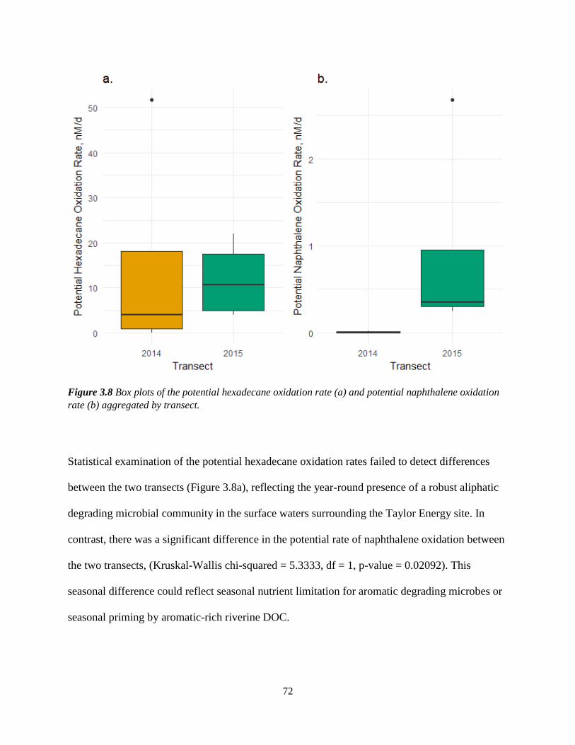
72

Figure 3.8 Box plots of the potential hexadecane oxidation rate (a) and potential naphthalene oxidation

rate (b) aggregated by transect.

Statistical examination of the potential hexadecane oxidation rates failed to detect differences

between the two transects (Figure 3.8a), reflecting the year-round presence of a robust aliphatic

degrading microbial community in the surface waters surrounding the Taylor Energy site. In

contrast, there was a significant difference in the potential rate of naphthalene oxidation between

the two transects, (Kruskal-Wallis chi-squared = 5.3333, df = 1, p-value = 0.02092). This

seasonal difference could reflect seasonal nutrient limitation for aromatic degrading microbes or

seasonal priming by aromatic-rich riverine DOC.

73

3.3.3.3 Rate Constants for Hydrocarbon Turnover Assays

To further examine the rates, we can also examine the rate constant, k, as measured by the

radiotracer assays (Equations 3.2 and 3.3). The rate constant is the quotient of alpha (fraction of

total radiotracer turned over to 14CO2 out of the total pool injected into the live incubation,

corrected for kill controls and instrument blanks) and incubation time. Examination of the rate

constant allows us to compare potential rates across the Taylor Energy site independently of the

measured in situ substrate concentration.

3.3.3.3.1 Hexadecane Oxidation Rate Constant

Examination of the hexadecane oxidation rate constants revealed a significant difference

between the two different transects (Kruskal-Wallis chi-squared = 4.0833, df = 1, p-value =

0.04331); examination by a Wilcox rank sum failed to detect a difference between the two

transects (Wilcoxon rank sum test; p-value= 0.05714). No significant differences were detected

with each transect.

Figure 3.9 Rate constants for hexadecane oxidation, plus or minus the standard deviation among the

radiotracer replicates. Bars are colored according to the year the sample was taken.

74

3.3.3.3.2 Naphthalene Oxidation Rate Constant

The only significant difference across naphthalene oxidation rate constants was detected between

the two transects (Kruskal Wallis rank sum test: Kruskal-Wallis chi-squared = 5.4634, df = 1, p-

value = 0.01942). A follow up examination with a Wilcoxon rank sum test agreed with this

finding (Wilcoxon rank sum test: p-value=0.02843), agreeing with the potential rate finding

discussed earlier.

Figure 3.10 Rate constants for naphthalene oxidation, plus or minus the standard deviation among the

radiotracer replicates. Bars are colored according to the year the sample was taken.

Analysis of the rate constant largely agrees with the analysis of the full potential rate data. There

are significant differences in the microbial community's ability to mineralize hydrocarbons

across seasons, but not within each transect. The major difference is with respect to hexadecane

oxidation; analysis of the potential rate revealed no significant differences between the autumn

2014 and summer 2015 transect, yet there were significant differences with respect to the rate

constant (Kruskal-Wallis chi-squared = 4.0833, df = 1, p-value = 0.04331).

75

3.4 Discussion

3.4.1 Commentary about post hoc experimental design

The comparison between these two transects is truly a post hoc experimental design utilizing

samples of opportunity, and there are considerable concerns with this. The sample sizes for each

station are different across the years (n=1/ station in 2014; n= 3 /station in 2015).

The 2014 samples included in this project are some of the very first biological and geochemical

samples collected from surface waters at the Taylor Energy site. Unfortunately, for this transect,

we were water-limited in our sampling, with only one sample taken per station. We were unsure

of what kind of variability we might see within these four stations within this single transect. As

such, sampling was rethought and redesigned prior to the 2015 transect.

The 2015 transect, again, has some interesting factors to consider. According to the CGMIX

database, there was an oil slick (2 km x 0.5 km; SEQNOS report ID 1119149) reported slick at

the Taylor Energy site, following a northwest to southeast trajectory the day of sampling.

However, between the time of the slick sighting and getting on station, a storm rolled through,

severely limiting any slick visibility and likely breaking up any slicks that had previously set up

during the day.

3.4.2 Comparison of Potential Hydrocarbon Oxidation Rates

3.4.2.1 Differences between Substrates

Previously, hydrocarbon oxidation rates were compared amongst each other siloed the rates by

the type of rate. However, these rate methods were developed as tools to quantify the

biodegradation of a complex mixture of petroleum hydrocarbons in surface water. Ultimately, we

76

hope to compare these two types of potential rates to better understand the fate of the various

fractions of petroleum hydrocarbons in the environment.

Overall, there are higher rates of hexadecane oxidation compared to naphthalene oxidation in

surface waters around the Taylor Energy site (Wilcoxon rank sum test: p-value= 0.03226). The

mean potential hexadecane oxidation rate is 13.40 nM/d compared to the mean potential

naphthalene oxidation rate of 0.46 nM/d. This nearly two orders of magnitude difference agrees

with previously work; Aeppli et al. described n-alkanes as among the most readily biodegraded

classes compounds within oil (Aeppli et al. 2014). Moreover, the mineralization of hexadecane

requires breaking single carbon-carbon bond, where each carbon is bound to one another across a

pair sp3 hybridized orbitals. The mineralization of naphthalene requires breaking double carbon-

carbon bonds, which require enough energy to break both the single bond forged from the two

sp3 hybridized orbitals as well as the pi bond that contributes to the compounds aromaticity. This

difference in bond structure is echoed in the energetic costs to break these different kinds of

carbon bonds: 348 kJ/mol for saturated carbon bonds, compared to 519 kJ/mol required for a

single carbon aromatic bond (Silverstein et al., 2005).

Constraining these hydrocarbon oxidation rates is important to the much larger study of how oil

is transformed biologically. While the biodegradation of mid-sized alkanes has long been

characterized, it has been assumed that the disappearance of aromatic hydrocarbons from surface

slicks was largely the result of physical processes, such as evaporation, photo-oxidation,

oxidation, and/or dissolution. It appears, however, that biodegradation of a small aromatic, like

naphthalene, is an important sink for these petroleum hydrocarbons.

77

3.4.2.1 Differences between Fall 2014 and Summer 2015 Transects

Previously, we established that there are seasonal differences in the slick length and frequency at

the Taylor Energy site and that the northern Gulf of Mexico is a highly seasonal region. The first

installment of this chapter illustrated that these seasonal differences are also apparent at the

Taylor Energy site. Closer examination of the rate data has revealed a significant difference with

respect to the potential rate of naphthalene oxidation between the two transects (Kruskal-Wallis

chi-squared = 5.3333, df = 1, p-value = 0.02092), but not the potential rate of hexadecane

(Kruskal-Wallis chi-squared = 1.3333, df = 1, p-value = 0.2482). Unlike hexadecane, the

potential rate and the rate constant data agree for naphthalene oxidation.

One question that emerges from this work is whether the rates of hydrocarbon oxidation differ

with season at the Taylor Energy site. While the data included in this chapter are not rich enough

to definitively describe the seasonal differences for all petroleum hydrocarbons, we can begin to

understand how the microbial community and its capacity to degrade broad classes of

hydrocarbons changes between the summer and autumn months. If hexadecane is a good model

for other mid-sized normal alkanes, then there appears to be no seasonal variation with respect to

the potential rate of biodegradation for these compounds. The significant increase in naphthalene

oxidation in the summer 2015 transect as compared to the fall 2014 transect suggests that there

may be seasonal controls on the biodegradation of small aromatic compounds. While these

trends are suggestive, there is not enough information to assess whether oil is biodegraded more

rapidly in the autumn or summer based on just these two transects. Sampling the site, with and

without oil, across various points of time in the year will be required to ultimately state if there

are significant seasonal microbial sinks of petroleum hydrocarbons in the surface waters at the

Taylor Energy site. Understanding the seasonal capacity of microbial oxidation of oil in surface

78

waters around the Taylor Energy site is important for understanding the greater ecological

impact of the Taylor Energy oil spill to coastal waters. For instance, economically valuable and

large predatory pelagic species, such as blue- and yellowfin tuna, amberjack, sailfish, blue

marlin, and cobia spawn offshore in the late spring and summer months, and can be significantly

impacted by trace concentrations of crude oil in the water column (Incardona et al. 2013;

references 5-13 therein).

3.4.3 Correlations between Nutrients and Potential Hydrocarbon Oxidation Rates

Examining the geochemical and potential rate data from across both transects via a Spearman’s

Rank Correlation test allows us to hypothesize which geochemical parameters could be candidate

drivers for hydrocarbon oxidation in surface waters (Figure 3.11).

Given that there were no statistical differences between the two transects with respect to

potential hexadecane oxidation rates, it is unsurprising that there were also no significant

correlations between potential hexadecane oxidation rates and any of the other geochemical

parameters tested that varied significantly. There were, however, significant relationships

between parameters used to calculate the rate, including the rate constant (HexaOx.RC) and the

potential rate using just tracer concentration (HexaOx.Tracer). There was a strong negative

correlation between potential hexadecane oxidation rates and ammonium, but this relationship

was not found to be significant (Spearman’s rank correlation: rho = -0.59; p-value = 0.1233).

There were several statistically significant relationships between the potential rate of naphthalene

oxidation and dissolved nutrients. The potential rate of naphthalene oxidation was positively

correlated with nearly every geochemical parameter measured: phosphate concentrations

(Spearman’s rank correlation: rho = 0.88; p-value = 0.00361), nitrate concentrations (Spearman’s

79

rank correlation: rho = 0.86; p-value = 0.00628), total dissolved nitrogen (Spearman’s rank

correlation: rho = 0.84; p-value = 0.00949), total dissolved phosphate (Spearman’s rank

correlation: rho = 0.83; p-value = 0.00997); nitrite (Spearman’s rank correlation: rho = 0.77; p-

value = 0.02681); and DOC (Spearman’s rank correlation: rho = 0.80; p-value = 0.01654). There

was no significant relationship between naphthalene oxidation and ammonium concentrations.

Meanwhile, there was a negative relationship between naphthalene oxidation and total petroleum

hydrocarbon concentration (Spearman’s rank correlation: rho = -0.79; p-value = 0.01937) as well

as with measured quantities of naphthalene, although the latter correlation was not statistically

significant (Spearman’s rank correlation: rho = -0.59 ; p-value = 0.125).

Naphthalene oxidation is significantly correlated with higher concentrations of dissolved

nitrogen and phosphate species, indicating that naphthalene oxidation may become nutrient

limited in fall and winter months.

Naphthalene oxidation also appears to have a complex relationship with carbon in surface

waters. While there is a statistically significant negative relationship between the concentration

of oil at a site and the rate of naphthalene oxidation (Spearman’s rank correlation: rho = -0.79; p-

value = 0.01937), there is also a statistically significant and equally positive correlation with

dissolved organic carbon across the site (Spearman’s rank correlation: rho = 0.80; p-value =

0.01654). The negative relationship with oil and naphthalene oxidation may stem from

synergistic toxicity or higher affinity for smaller aromatic compounds. More likely, this negative

relationship reflects that the stations with heavily oiled surface water were also nutrient limited.

Further investigations at the Taylor Energy site are needed to understand the relationship

between oil concentrations and potential naphthalene oxidation rates.

80

The significant, positive relationship between DOC and potential rates of naphthalene oxidation

is among the most surprising discoveries from this site. This relationship may reflect an

underlying influence of the Mississippi River plume on the surface waters at the Taylor Energy

site. As conduits of carbon from terrestrial to marine ecosystems, rivers play a key role in the

transformation of terrestrial carbon to marine carbon. One important class of terrestrial carbon is

lignin, a key component in the support structure of woody plants, comprised of phenolic

compounds joined together with aromatic ether bonds. Lignin is heavily degraded along riverine

systems, such as the Amazon River (Ward et al. 2013), releasing small aromatic compounds,

such as phenols, into the DOC pool. Microbial communities along the river-ocean-continuum

responsible for this transformation has been implicated as an important sink for these aromatic

compounds, especially at a river’s mouth (Medeiros et al. 2015). The export of degraded

terrestrial carbon and the microbial communities responsible for degrading terrestrial material

may confer the Taylor Energy site, a site inundated with persistent oil slicks, with a microbial

community primed to degrade small aromatic compounds found in oil, such as naphthalene.

81

Figure 3.11 Correlogram of all rates and geochemical parameters from the in situ sampling regime of

the Taylor Energy site, using a Spearman's rank correlation test. Rho values are depicted as colors; blue

values indicate a positive relationship, white bubbles indicate a neutral or minimal relationship, and red

values indicate a negative relationship.

82

3.5 Conclusion

These two transects conducted in the fall and summer represent two extreme ends of the

biogeochemical range possible at the Taylor Energy site. While this is not a full factorial

exploration of this site (with oil across all four seasons; without oil across all four seasons), these

two transects reveal the surface water at the Taylor Energy site to be a highly dynamic and

seasonally variant site. There were significant differences with respect to dissolved nutrients and

the potential naphthalene oxidation rate between the summer and fall transects, but the potential

rate of hexadecane was robust and not significantly different between the two transects. No

significant differences were found within transects, but deeper sampling will be required to

resolve nutrient and hydrocarbon degrading dynamics within the area of a surface slick.

Differences in correlations between dissolved nutrients and potential hydrocarbon oxidation rates

suggest that the geochemical controls governing hydrocarbon oxidation in surface waters are

highly substrate specific and may be seasonally variant.

83

References

Aeppli, C.; Carmichael, C. A.; Nelson, R. K.; Lemkau, K. L.; Graham, W. M.; Redmond, M.

C.; Valentine, D. L.; Reddy, C. M. Oil Weathering after the Deepwater Horizon Disaster

Led to the Formation of Oxygenated Residues. Environ. Sci. Technol. 2012, 46 (16),

8799–8807 DOI: 10.1021/es3015138.

Aeppli, C.; Nelson, R. K.; Radovic, J. R.; Carmichael, C. A.; Valentine, D. L.; Reddy, C. M.

Recalcitrance and Degradation of Petroleum Biomarkers upon Abiotic and Biotic

Natural Weathering of Deepwater Horizon Oil. Environ. Sci. Technol. 2014, 48, 6726–

6734.

Bendschneider K.; Robinson R.J. A new spectrophotometric method for the determination of

nitrite in sea water. University of Washington Oceanographic Laboratories. 1952.

Braman, R.S.; Hendrix, S.A. Nanogram nitrite and nitrate determination in environmental and

biological materials by vanadium (III) reduction with chemiluminescence detection.

Analytical Chemistry. 1989 Dec 1;61(24):2715-8.

Garside C. A chemiluminescent technique for the determination of nanomolar concentrations of

nitrate and nitrite in seawater. Marine Chemistry. 1982 Apr 1;11(2):159-67.

Harrison, S.J. Investigating the Dynamic Range of Weathered Oil and Chemical Dispersant in

the Environment. B.Sc. Thesis, Haverford College, Haverford, PA. 2013.

Incardona, J. P.; Gardner, L. D.; Linbo, T. L.; Brown, T. L.; Esbaugh, A. J.; Mager, E. M.;

Stieglitz, J. D.; French, B. L.; Labenia, J. S.; Laetz, C. A.; Tagal, M.; Sloan, C. A.;

Elizur, A.; Benetti, D. D.; Grosell, M.; Block, B. A.; Scholz, N. L. PNAS Plus: From the

Cover: Deepwater Horizon Crude Oil Impacts the Developing Hearts of Large Predatory

Pelagic Fish. Proc. Natl. Acad. Sci. 2014, 111 (15), E1510–E1518 DOI:

10.1073/pnas.1320950111.

Kleindienst, S.; Seidel, M.; Ziervogel, K.; Grim, S.; Loftis, K.; Harrison, S.; Malkin, S. Y.;

Perkins, M. J.; Field, J.; Sogin, M. L.; Dittmar, T.; Passow, U.; Medeiros, P. M.; Joye,

S. B. Chemical Dispersants Can Suppress the Activity of Natural Oil-Degrading

Microorganisms. Proc. Natl. Acad. Sci. 2015, 112 (48) DOI: 10.1073/pnas.1507380112.

Kozich, J. J.; Westcott, S. L.; Baxter, N. T.; Highlander, S. K.; Schloss, P. D. Development of a

Dual-Index Sequencing Strategy and Curation Pipeline for Analyzing Amplicon

Sequence Data on the Miseq Illumina Sequencing Platform. Appl. Environ. Microbiol.

2013, 79 (17), 5112–5120 DOI: 10.1128/AEM.01043-13.

84

Liu, Y.; Kujawinski, E. B. Chemical Composition and Potential Environmental Impacts of

Water-Soluble Polar Crude Oil Components Inferred from ESI FT-ICR MS. PLoS One

2015, 10 (9), e0136376 DOI: 10.1371/journal.pone.0136376.

Medeiros, P.; Seidel, M.; Ward, N. D.; Carpenter, E.; Gomes, H.; Niggemann, J.; Krusche, A.

V; Richey, J. E.; Yager, P. L.; Dittmar, T. Fate of the Amazon River Dissolved Organic

Matter in the Tropical Atlantic Ocean. Global Biogeochem. Cycles 2015, 677–690 DOI:

10.1002/2015GB005115.

Pearlman R.S.; Yalkowsky, S.H.; Banerjee S. Water solubilities of polynuclear aromatic and

heteroaromatic compounds. Journal of physical and chemical reference data. 1984

Apr;13(2):555-62.

Sibert, R. J.; Harrison, S. J.; Joye, S. B. Protocols for Radiotracer Estimation of Primary

Hydrocarbon Oxidation in Oxygenated Seawater. In Hydrocarbon and Lipid

Microbiology Protocols; McGenity, T. J., Timmis, K. N., Nogales, B., Eds.; Humana

Press, 2016; pp 263–276.

Silverstein, R.M.; Webster, F.X.; Kiemle, D.J. Spectrometric Identification of Organic

Compounds, 7th ed.; John Wiley & Sons, Inc.: Hoboken, 2005.

Solorzano L. Determination of ammonia in natural waters by phenolhypochlorite method 1 1.

This research was fully supported by US Atomic Energy Commission Contract No.

ATS (11‐1) GEN 10, PA 20. Limnology and Oceanography. 1969 Sep 1;14(5):799-801.

Solorzano, L.; Sharp, J. H. Determination of Total Dissolved Phosphorous and Particulate

Phosphorous in Natural Waters. Limnol. Ocean. 1980, No. 1965, 754–758.

Ward, N. D.; Keil, R. G.; Medeiros, P. M.; Brito, D. C.; Cunha, A. C.; Dittmar, T.; Yager, P. L.;

Krusche, A. V.; Richey, J. E. Degradation of Terrestrially Derived Macromolecules in

the Amazon River. Nat. Geosci. 2013, 6 (7), 530–533 DOI: 10.1038/ngeo1817.

85

CHAPTER 4

AVAILABILITY OF DISSOLVED NUTRIENTS AND CHEMICAL DISPERSANT

IMPACTS MICROBIAL COMMUNITIES AND POTENTIAL HYDROCARBON

OXIDATION RATES IN SURFACE WATER FROM THE TAYLOR ENERGY SITE

4.1 Introduction

When oil is spilled in a coastal or marine environment, first responders are often left with a

selection of difficult choices about how to respond to the spilled oil. Physical efforts to contain

and divert the oil from delicate coastal environments can include deploying booms, packed with

oil absorbing materials, or skimming sheens off the surface. Responders have also used

controlled in situ burning of surface slicks to remove surface slicks. The efficacy of these

mitigation efforts can be limited by the amount of oil spilled, the location of the spill, the

weather conditions at the site of the spill, and the type of oil spilled (e.g. bunker fuel, crude oil,

etc.) (Daling and Lewis, 2001).

Chemical dispersants, complex mixtures of solvents and surfactants able to physically lower the

free energy at the interface between nonpolar and polar molecules, were first applied in the

aftermath of the 1967 Torrey Canyon oil spill. An estimated 136 million liters of oil washed

onshore after an oil tanker ran aground on Seven Stones reef, located off the southwest coast of

England. At the time, it was the considered the largest oil spill in history. 10,000 tons of first

generation dispersants were applied on delicate shoreline ecosystems to clean up the oil, killing

86

scores of sea birds, threatening the local commercial fisheries, and upsetting the coastal

ecosystem for decades (Southward and Southward, 1978).

Since their first use, various formulations of dispersants have been used in the cleanup efforts of

many notable oil spills, including the 1977 Ekofisk Bravo blow out in the North Sea, the 1993

Braer spill off the Scottish coast, the 1996 Sea Empress spill off the English coast (Daling and

Lewis, 2001), and most recently during the 2010 Deepwater Horizon blow out in the northern

Gulf of Mexico.

Yet, many questions remain about the impact of these chemical mixtures. There is little dispute

that dispersants function well at the molecular level to break up oil slicks and remove oil from

the sea surface. Prince et al. (2015), however, heralded these mixtures as “bioremediation

tool[s]”, which stimulate aerobic oil degradation through the process of dilution, overcoming

macronutrient and oxygen limitation in surface waters. McFarlin et al. (2014) demonstrated that

0.167 ppm addition of Corexit 9500, the primary chemical dispersant used in the Deepwater

Horizon oil spill response, enhanced the rate of oil degradation compared to undispersed oil

treatment at each time point up until the end of their 60-day incubation of Arctic surface waters

(McFarlin et al. 2014). Kleindienst et al. (2015) demonstrated that chemical dispersants do not

stimulate, and in some cases, may suppress the activity of natural oil-degrading microorganisms

in Gulf of Mexico mid-waters (Kleindienst et al. 2015).

It has long been known that microbial communities in surface waters readily respond to oil

(Atlas 1981, Leahy and Colwell, 1990), and dissolved nutrients enhance the capabilities of oil

degrading microbial communities (Atlas 1981, Leahy and Colwell 1990, Prince 2010). Without

these inorganic nutrients, microbial communities have few resources to breakdown carbon rich

oil in surface slicks. Edwards et al. (2011) postulated that offshore nutrient limitation inhibited

87

the degradation of oil in surface slicks in the aftermath of the Deepwater Horizon oil spill.

Meanwhile, Seidel et al. documented the disappearance of heteroatomic compounds from a

WAF bottle experiment, indicating some of the metabolic plasticity microbial communities use

to work around apparent nutrient limitation to degrade petroleum derived hydrocarbons (Seidel

et al. 2015).

Moreover, little is known about the nutrient dynamics following application of Corexit to surface

waters. In this chapter, we will compare the microbial response of a chemical dispersant, Corexit

9500A (Nalco, Sugar Land, TX), with an inorganic nutrient amendment (NO3-, NH4

+, HPO43-,

20:1 N:P) in surface waters from the Taylor Energy site in the northern Gulf of Mexico. We will

explore how inorganic nutrients are utilized in these different treatments, how potential

hydrocarbon oxidation rates change, and how microbial communities change after application of

chemical dispersant and nutrients.

4.2 Methods and Materials

4.2.1 Sample Collection

Surface waters from four stations approaching the Taylor Energy site in the northern Gulf of

Mexico were collected via bucket cast on board the RV Endeavor, aliquoted into 1L bottles.

Although an oil slick had been spotted near the site (SEQNOS ID: 1119149) several hours before

we arrived on station, a summer storm had churned up the slick prior to our arrival on station. No

oil sheen or smell was visible in any of the four stations along the transect (Figure 4.1).

88

Figure 4.1 Map of the Taylor Energy Site in the northern Gulf of Mexico. Regional overview from Google

Maps (left); satellite image of the site with oil emanating from the source, demarcated with an X (top

right); and a map of surface water sampling locations (shades of blue) featured in this chapter (bottom

right).

4.2.2 Experimental Design

Water from each station was aliquoted into 1L amber bottles and amended with one of the

following treatments: + Nutrients (10μM NH4+

, 10 NO3- μM, and 1 μM HPO4

3-,) targeting a 20:1

N:P ratio; + Corexit (5 μL of Corexit 9500A); or Nutrients + Corexit, in triplicate, with an

unamended control for each station. Water was incubated for 24 h at room temperature onboard,

and sampled for dissolved nutrients, cell counts, potential hydrocarbon oxidation rates, and

hydrocarbon composition. 250 mL of each bottle was pooled with site and treatment replicates

for microbial community analysis via 16S rRNA sequencing.

89

Figure 4.2 Schematic of experimental design (a) and sampling design (b). Surface water was collected

from each of the four stations, and was sampled for in situ values and rates. Additional surface water was

collected for the amendment experiment discussed here, with each treatment done in triplicate for each

station. Each bottle was sampled for cell counts and virus like particle counts, dissolved nutrients, DOC,

and water was subsampled for radiotracer assays. Water was pooled from each site and treatment for 16S

rRNA analysis (*).

4.2.3 Dissolved Nutrients

Aliquots of whole water were filtered (0.2 μm) and preserved at -20°C for analysis of dissolved

organic carbon (DOC), ammonium (NH4+), NOx

- (NO3- + NO2

-), total dissolved nitrogen (TDN),

phosphate (HPO43-), and total dissolved phosphate (TDP). Dissolved organic nitrogen and total

dissolved organic phosphate concentrations were estimated from subtraction of inorganic species

from total dissolved species.

Dissolved organic carbon (DOC) was analyzed by high temperature (680°C) combustion

catalytic oxidation on a total organic carbon analyzer (Shimadzu TOC-Vcph); concentrations

90

were determined by comparison to a series of potassium hydrogen phthalate standards. Organic

carbon was measured as the non-purgeable organic carbon (NPOC) content with an NDIR

detector, following sparging with phosphoric acid. Total dissolved nitrogen (TDN) was

measured on the same instrument with a TNM-1 module; concentrations were derived from a

glycine standard. Samples were not diluted prior to analysis.

Nitrate plus nitrite (NOx-) concentrations were quantified by a vanadium reduction method using

a vanadium reduction assembly (Antek 745; Braman and Hendrix, 1989) coupled with a

chemiluminescent nitric acid detector (Antek 7050; Garside et al. 1982).

Nitrite (NO2-) was analyzed in parallel by standard colorimetric assay (Bendschneider and

Robinson, 1952), while ammonium was measured colorimetrically using the standard phenol

hypochlorite method (Solorzano, 1969). Nitrate (NO3-) was determined from the subtraction of

NO2- from NOx

-.

Dissolved phosphate was measured colorimetrically, using the molybdate blue method

(Solorzano and Sharp, 1980). Total dissolved phosphate (TDP) was first precipitated with

magnesium sulfate, and heated with acid to convert organic phosphate into orthophosphate. This

residue was then subjected to colorimetric analysis using the molybdate blue method (Solorzano

and Sharp, 1980). Colorimetric analyses were performed using a Shimadzu UV-1601

spectrophotometer. Dissolved organic carbon (DOC) was analyzed by high temperature (680°C)

combustion catalytic oxidation on a total organic carbon analyzer (Shimadzu TOC-Vcph), as

compared to a series of potassium hydrogen phthalate solution standards. Samples were diluted

2:11 in Milli-Q water. Organic carbon was measured as the non-purgeable organic carbon

(NPOC) content with an NDIR detector, following sparging with a strong acid.

91

4.2.4 Hydrocarbons

Whole unfiltered water was frozen at -20° for analysis of total extractable hydrocarbons using a

method adapted from Kleindeisnt et al. (2015) and Kujawinski et al. (2014). Following thawing,

sample volume was determined gravimetrically, and spiked with known quantities of three

deuterated standards (5μg/sample; fluorene-d10, eicosane-d24, and benzo[a]pyrene-d12). Samples

were transferred to combusted 1L separation funnels fitted with solvent rinsed PTFE spigots, and

extracted with dichloromethane (2x 250 mL each) and hexane (1 x 250 mL). Samples from

stations A and D required additional hexane and dichloromethane washes as there were still

visible sheens of colored oil in the extraction. Organic fractions were combined and reduced in

volume via rotary evaporation (Buchi Corp.) and solvent exchanged into hexane. Samples were

further reduced to 500 μL under a gentle stream of Ar.

Organic extracts were analyzed with a gas chromatography with time of flight mass spectrometry

(GC-TOF-MS; Pegasus 4D GC, LECO, Michigan). 1 μL of each extract was injected with a 1:10

split injection method, and separated on two in-line columns; the primary column was a Rxi-5 Sil

fused silica column (60m x 0.25 mm ID; 0.25μm df; Restek) joined to an Rxi-17 Sil MS fused

silica column (1m x 0.10mm ID x 0.1μm dr; Restek) housed in a secondary GC oven. The GC

oven was held for 3 minutes at 50°C, followed by a 6°C/minute temperature ramp until reaching

320°C, and held for 20 minutes. Time of flight mass spectrometry allowed for the simultaneous

monitoring of ions ranging from 50-575 m/z across the entire method, after a 600 s solvent delay.

Samples were run alongside a standard curve of n-alkanes (nC7-nC40; heptane- tetracontane), a

mixture of 16 parent PAHs, and a dilution of crude oil as an estimation of total petroleum

hydrocarbons (TPH).

92

4.2.5 Potential Hydrocarbon Oxidation Rates

Potential hydrocarbon oxidation rates were quantified as the rate of conversion of a radiolabeled

model hydrocarbon into 14CO2 by the microbial community within each bottle (Kleindienst et al.

2015; Sibert et al. 2016). [1-14C]-n-hexadecane was used as the model aliphatic compound, and

[1,4,5,8-14C] naphthalene was used as the model aromatic compound.

Figure 4.3 Structures of 14C substrates used to quantify hydrocarbon turnover in surface waters. [1-14C]-

n-hexadecane (a) was used as a model linear alkane, and [1,4,5,8-14C] naphthalene was used as a model

aromatic compound (b).

Homogenized water from each microcosm was subsampled into headspace-free, 8mL glass

scintillation vials capped with a PTFE-lined rubber septum (Supelco, Pennsylvania). Each assay

was carried out in triplicate alongside a NaOH killed control. 14C-labeled hydrocarbons were

each dissolved in molecular grade ethanol and delivered into each scintillation vial with a glass

syringe (0.5 μCi=1.35 x 10-5 Bq; 10μL) and shaken gently to distribute the tracer. Killed controls

were injected with tracer and immediately added to the killing solution (2M NaOH, 2mL).

Incubations were carried out at room temperature in the dark, and stopped in the same manner as

killed controls. Assays were stored in the basic solution (pH> 10) at room temperature for up to 3

weeks before acidic distillation of the evolved 14CO2.

Evolved 14CO2 was distilled from the terminated incubation in the following method (Figure

3.3). Samples were transferred to 250mL Erlenmeyer flasks capped with rubber stoppers and

93

clamps and shaken with activated charcoal (1g, Sigma Aldrich) for 6h as a pre-treatment to bind

any unused tracer to the charcoal. Hexadecane oxidation assays were further amended with C18

reverse phase silica gel (250 mg, Supelco) to more effectively bind unused alkane tracer.

Figure 4.4 Schematic of hydrocarbon oxidation rate method developed by Kleindienst et al. (2015) and

Sibert et al. (2016).

Following this pretreatment, the Erlenmeyer flask was fitted with a carbon dioxide trap (1.5 mL,

CarboSorb E®, Perkin Elmer), acidified with concentrated phosphoric acid (5mL), and quickly

stoppered to minimize loss of evolved CO2. Acidified solutions were then shaken overnight to

capture CO2. Radioactivity of the carbon dioxide trap was quantified using a Beckman 6500

liquid scintillation counter, after adding scintillation fluid, (4.5mL, Scintisafe®, Fisher

Scientific) to each trap. Instrumentation blanks were counted after every 10 samples, and total

injected tracer was quantified as the blank corrected average of the 3 injections made into

scintillation fluid at the time of the incubation. All values from the scintillation counter were first

94

blank corrected, and each sample was kill corrected with the value of the kill control for each

sample.

Potential rates were calculated using modifications of the following formula (Equation 3.1). k is

the rate constant, a term derived from the quotient of α, the fraction of radiotracer turned over, by

t, the duration of the incubation. S is the concentration of the substrate.

−𝑑[𝐻𝑦𝑑𝑟𝑜𝑐𝑎𝑟𝑏𝑜𝑛]

𝑑𝑡= 𝑘[𝑆] = 𝛼

𝑡[𝑆] ∗

[𝑅𝑎𝑑𝑖𝑜𝑎𝑐𝑡𝑖𝑣𝑖𝑡𝑦 𝑡𝑢𝑟𝑛𝑒𝑑 𝑜𝑣𝑒𝑟, 𝑑𝑝𝑚]

[𝑅𝑎𝑑𝑖𝑜𝑎𝑐𝑡𝑖𝑣𝑖𝑡𝑦 𝑎𝑑𝑑𝑒𝑑, 𝑑𝑝𝑚]∗ [𝑆]

𝑡

Equation 4.1

Potential Hexadecane Oxidation Rate: [1-14C]-hexadecane + O2 14CO2 + H2O

−𝑑[𝐻𝑒𝑥𝑎𝑑𝑒𝑐𝑎𝑛𝑒]

𝑑𝑡= 𝑘[𝐻𝑒𝑥𝑎𝑑𝑒𝑐𝑎𝑛𝑒] =

𝛼

𝑡∗ [𝐻𝑒𝑥𝑎𝑑𝑒𝑐𝑎𝑛𝑒] =

[ 𝐶14 𝑂2]

[ 𝐶14 − 𝐻𝑒𝑥𝑎𝑑𝑒𝑐𝑎𝑛𝑒 ∗ 𝑡]∗ [𝐻𝑒𝑥𝑎𝑑𝑒𝑐𝑎𝑛𝑒]

Equation 4.2

Potential Naphthalene Oxidation Rate: [1,4,5,8-14C]-naphthalene + O2 14CO2 + H2O

−𝑑[𝑁𝑎𝑝ℎ𝑡ℎ𝑎𝑙𝑒𝑛𝑒]

𝑑𝑡= 𝑘[𝑁𝑎𝑝ℎ𝑡ℎ𝑎𝑙𝑒𝑛𝑒] =

𝛼

𝑡∗ [𝑁𝑎𝑝ℎ𝑡ℎ𝑎𝑙𝑒𝑛𝑒] =

[ 𝐶14 𝑂2]

[ 𝐶14 − 𝑁𝑎𝑝ℎ𝑡ℎ𝑎𝑙𝑒𝑛𝑒 ∗ 𝑡]∗ [𝑁𝑎𝑝ℎ𝑡ℎ𝑎𝑙𝑒𝑛𝑒]

Equation 4.3

Calculated Concentration of the Radiotracer used in the 14C Incubations

The concentration of the added tracer is a function of the incubation vessel dimension (7.5 mL)

and specific activity of the hexadecane and naphthalene tracer, as determined by the

manufacturer (55 Ci/mol and 58 Ci/mol, respectively; Equations 4.2 and 4.3).

[𝐻𝑒𝑥𝑎𝑑𝑒𝑐𝑎𝑛𝑒 𝑡𝑟𝑎𝑐𝑒𝑟] =𝑅𝑎𝑑𝑖𝑜𝑎𝑐𝑡𝑖𝑣𝑖𝑡𝑦 𝑜𝑓 𝑎𝑑𝑑𝑒𝑑 𝑡𝑟𝑎𝑐𝑒𝑟, 𝑑𝑝𝑚

𝑉𝑜𝑙𝑢𝑚𝑒 𝑜𝑓 𝑖𝑛𝑐𝑢𝑏𝑎𝑡𝑖𝑜𝑛 𝑣𝑒𝑠𝑠𝑒𝑙, 𝑚𝐿∗

1 𝑚𝐶𝑖

2.22𝑥109𝑑𝑝𝑚∗

1𝑚𝑚𝑜𝑙

55 𝑚𝐶𝑖

Equation 4.4

[𝑁𝑎𝑝ℎ𝑡ℎ𝑎𝑙𝑒𝑛𝑒 𝑡𝑟𝑎𝑐𝑒𝑟] =𝑅𝑎𝑑𝑖𝑜𝑎𝑐𝑡𝑖𝑣𝑖𝑡𝑦 𝑜𝑓 𝑎𝑑𝑑𝑒𝑑 𝑡𝑟𝑎𝑐𝑒𝑟, 𝑑𝑝𝑚

𝑉𝑜𝑙𝑢𝑚𝑒 𝑜𝑓 𝑖𝑛𝑐𝑢𝑏𝑎𝑡𝑖𝑜𝑛 𝑣𝑒𝑠𝑠𝑒𝑙, 𝑚𝐿∗

1 𝑚𝐶𝑖

2.22𝑥109𝑑𝑝𝑚∗

1𝑚𝑚𝑜𝑙

58 𝑚𝐶𝑖

Equation 4.5

95

The in situ concentrations of hexadecane and naphthalene were below the limit of detection via

GC-MS for the entire summer 2015 transect, and so the concentration of the tracer was used in

the radiotracer incubations was used to calculate the potential rate of hydrocarbon oxidation.

4.2.6 Microbial Community

Microorganism were filtered onto a Sterivex filter cartridge (0.22μm; Millipore) and flash frozen

in liquid nitrogen. Homogenized water from each biological replicate was pooled with other

station replicates for a total of 750 mL water per station (3 bottles/station * 250 mL/bottle= 750

mL). Samples were shipped on dry ice from Gulfport, MS to Athens, GA, and stored at -80C

until processing. Sterivex filters were thawed on ice, the tops removed with sterilized pliers, and

the filter cut using sterile scalpels; the cut filters were immediately processed for DNA extraction

using the DNeasy Powerwater Kit (Qiagen) according to the manufacturer’s directions. Eluted

DNA was quantified using the dsDNA assay kit and a Qubit fluorometer (Invitrogen) (Table

4.1).

Barcoded amplicons of the 16S rRNA were generated using primers amplifying the V4 region

and the AccuPrime Pfx SuperMix kit (Invitrogen) with methods previously described (Kozich

et al. 2013; Table 3.2). Samples were sequenced on an Illumina MiSeq (Illumina) at the Georgia

Genome Facility (GGF, University of Georgia, Athens, GA) resulting in 2x250 paired-end reads.

At the time of writing, analyses of these data were still underway and will not be discussed

further.

96

4.2.7 Statistical Analysis

Data was analyzed using R version 3.2.4 (Copyright (C) 2016, The R Foundation for Statistical

Computing). Due to the small sample size and non-normal distributions of data, non-parametric

tests were used to compare and contrast the biogeochemical data from the two stations. Variance

was assessed by the Kruskal-Wallis Rank Sum Test, a non-parametric alternative to an ANOVA.

Paired Wilcox rank sum tests were used to assess differences within the sample sets, and

Spearman’s rank coefficients were used to assess correlation between geochemical parameters.

4.3 Results

4.3.1 Dissolved Nutrients

4.3.1.2 Dissolved Nitrogen

As a coastal station 18 km the mouth of the Mississippi River, there are high levels of total

dissolved nitrogen (TDN) at this station during the spring-summer months compared with farther

offshore (Edwards et al. 2011 and Pomeroy et al. 1995).

A Kruskal-Wallis rank sum test detected a difference in ammonium drawdown by treatment

(Kruskal-Wallis chi-squared = 10.201, df = 3, p-value = 0.01693), and a series of Wilcoxon rank

sum tests detected a significant difference in the drawdown of ammonium in the Nutrient +

Corexit treatment compared to the unamended treatment (p-value = 0.02021). In the Nutrient +

Corexit treatments, nearly the entire ammonium addition (10 μM) was depleted over the 24 h

incubation.

97

Figure 4.5 Bar plots of the dissolved nitrogen species grouped by treatments and shaded by station after

incubation for 24h with each respective treatment. C= Corexit alone, N= + Nutrients, NC= Corexit +

Nutrients, U= unamended controls. Colors progressing from pale blue to dark blue as a function of

moving away from the Taylor Energy site.

Figure 4.6 Bar plots of ammonium drawdown (a) and total dissolved nitrogen drawdown (b) grouped by

treatments and shaded by sites after incubation for 24h with each respective treatment. C= Corexit alone,

N= + Nutrients, NC= Corexit + Nutrients, U= unamended controls. Colors progressing from pale blue to

dark blue as a function of moving away from the Taylor Energy site.

98

A Kruskal-Wallis rank sum test detected a difference in the drawdown of total dissolved nitrogen

by treatment (Kruskal-Wallis chi-squared = 11.707, df = 3, p-value = 0.008458), and a series of

Wilcoxon rank sum tests detected a significant difference in the drawdown of total nitrogen in

the Nutrient+ Corexit treatments compared to the unamended controls (p-value = 0.0294) as well

as in the Corexit amended treatments (W = 0, p-value = 0.02843). No significant difference was

observed between the nutrient amended treatment and the unamended controls.

Dissolved nitrogen species were significantly removed in all Corexit-amended treatments, and

ammonium was significantly depleted in the nutrient + Corexit treatments.

4.3.1.2 Dissolved Organic Species

A Kruskal-Wallis rank sum test detected that there was a significant difference in the size of the

dissolved organic pool by treatment, and a follow up analysis with a Wilcox rank sum detected

significantly higher levels of DOC both Corexit amended treatments compared to unamended

treatments (Corexit alone: W = 144, p-value = 3.63e-05; Nutrients + Corexit: W = 144, p-value =

3.63e-05), a difference of about 100 μM on average. Analysis of the dissolved organic nitrogen

pool failed to reveal differences by treatment, indicating that the pool of dissolved organic

species is carbon rich. Given the dynamic range of compounds within the Corexit formulation

and its predominant hydrocarbon formulation (Harrison, 2013; Baelum et al. 2012), it is

unsurprising that many of these compounds enter the pool of dissolved organic carbon.

99

Figure 4.7 Bar plots of the dissolved organic carbon (DOC) and dissolved organic nitrogen (DON)

concentrations following 24h incubation with each respective treatment. Plots are grouped by treatments

and shaded by site. C= Corexit alone, N= + Nutrients, NC= Corexit + Nutrients, U= unamended

controls. Colors progressing from pale blue to dark blue as a function of moving away from the Taylor

Energy site.

4.3.1.3 Dissolved Phosphorous Species

As expected for surface waters, the background levels of orthophosphate and total dissolved

phosphate were close to 1μM, with no significant differences detected across the four stations

(Figure 4.4). A Kruskal-Wallis rank sum test detected a significant difference in the drawdown

of phosphate by treatment (Kruskal-Wallis chi-squared = 12.812, df = 3, p-value = 0.005061).

Follow-up analysis of the drawdown of phosphate revealed a significant difference in the

drawdown of phosphate in both Corexit-amended treatments compared to unamended treatments

(p-value = 0.02857; p-value = 0.02857; Figure 4.5). No significant difference in the drawdown

of phosphate was detected in the nutrient amended treatments.

100

Figure 4.8 Bar plots of phosphate (a) and total dissolved phosphate (TDP) species (b) grouped by

treatments and shaded by sites. C= Corexit alone, N= + Nutrients, NC= Corexit + Nutrients, U=

unamended controls. Colors progressing from pale blue to dark blue as a function of moving away from

the Taylor Energy site.

Figure 4.9 Bar plots of the phosphate drawdown grouped by treatments and shaded by sites. C= Corexit

alone, N= + Nutrients, NC= Corexit + Nutrients, U= unamended controls. Colors progressing from

pale blue to dark blue as a function of moving away from the Taylor Energy site.

101

4.3.4 Nutrient Summary

Taken together, the Corexit amendments (5 μL/1L; 5 ppm) significantly changed the size of the

dissolved organic carbon pool in these surface water incubations. It is important to note that this

concentration of Corexit is well below the estimated critical micelle concentration (CMC) of

Corexit estimated by Steffy et al. (2011) and in the same order of magnitude as the trace levels

of DOSS detected in midwater depths from 2010 in the aftermath of the Deepwater Horizon oil

spill (Kujawinski et al. 2011), if DOSS is ~10% by mass.

Over the course of the 24h incubation in the dark, there were significant differences in the

amount of total dissolved nitrogen and phosphate utilized in both Corexit-amended treatments

compared to the unamended treatment. This observation was not seen in the nutrient-only

treatments. This suggests that adding low amounts of Corexit changes the pool of carbon in

surface waters, which dramatically alters the way that nutrients are utilized, and that the change

is rapid, changing on timescales of hours. This change in nutrient use could make these

communities that are already at risk of being nutrient limited (Pomeroy 1995; Edwards 2011)

even more so and could limit the ability of these microbial communities to degrade petroleum

hydrocarbons found in surface waters.

102

4.3.2 Microbial Community Composition

Figure 4.10 Bar plots of the cell counts (a) and virus like particles (b) grouped by treatments and shaded

by sites. C= Corexit alone, N= + Nutrients, NC= Corexit + Nutrients, U= unamended controls. Colors

progressing from pale blue to dark blue as a function of moving away from the Taylor Energy site.

No significant differences in cell counts were detected across sites or treatments, and the only

significant difference with respect to virus like particles was detected between the nutrient

amended treatments and nutrient + Corexit amended treatments (W = 21, p-value = 0.003535).

However, given that neither treatment was significantly different from the controls, this is not a

treatment effect and may reflect a subtle shift in the dynamic responses to nutrients and

dispersant.

Analyses of the 16S rRNA data is still underway and is to be featured in future work.

4.3.3 Potential Hydrocarbon Oxidation Rates

4.3.3.1 Potential Hexadecane Oxidation Rates

There was robust oxidation of the hexadecane tracer across the whole Taylor transect, especially

compared to offshore stations in the Gulf of Mexico (Shepherd and Joye, unpublished results

from EN586). The nutrient amendment had the most dramatic impact at station G, which was the

most oligotrophic station among those featured in this study.

103

A Kruskal-Wallis rank sum test detected differences among the hexadecane oxidation rate by

treatment (Kruskal-Wallis chi-squared = 10.004, df = 3, p-value = 0.01853), however, there were

no significant differences in potential hexadecane oxidation were observed between the

unamended controls and the amended samples. Therefore, there is no treatment effect of Corexit

or nutrients on the potential rate of hexadecane oxidation after a 24 h exposure.

Figure 4.11 Bar plots of the potential hexadecane oxidation grouped by treatments and shaded by sites.

C= Corexit alone, N= + Nutrients, NC= Corexit + Nutrients, U= unamended controls. Colors

progressing from pale blue to dark blue as a function of moving away from the Taylor Energy site.

However, there were no significant differences between the amendment treatments. Between

nutrient only amendments and Corexit-only amendments, potential hexadecane oxidation rates

were higher in the nutrient amended samples (W = 21, p-value = 0.002316). Between the two

nutrient amended treatments, potential rates were higher among the nutrient-only amended

samples compared to the nutrient and dispersant treatment (W = 109, p-value = 0.03324). This

indicates that Corexit and dissolved nutrients have diverging impacts on the potential rate of

hexadecane oxidation in surface waters. In agreement with previous findings in mid-water

(Kleindeinst et al. 2015), Corexit does not enhance the rate of potential hexadecane oxidation in

104

surface waters, but, perhaps more importantly to oil spill responders, Corexit does not appear to

depress the potential rate of alkane degradation either. However, a longer incubation may be

required to detect significant differences from the unamended control treatments.

These findings can be explained for several reasons: Corexit, itself, has n-alkanes within its

formulation (Harrison, 2013; Baelum et al. 2013; Nalco MSDS, 2012), and so microorganisms

may prefer to degrade these shorter, more labile n-alkanes over the radiolabeled n-hexadecane.

Alternatively, it is possible that the added substrate, hexadecane, was intermolecularly bound to

components of the dispersant (e.g. surfactants and solvents) through alkyl-alkyl interactions,

which become important intermolecular forces in the presence of increasingly polar solvents

(Yang et al. 2013). Nutrient data from this data set, however, suggests the former, given the

significant drawdown of nutrients in Corexit-amended treatments suggests that something is

being degraded.

4.3.3.2 Potential Naphthalene Oxidation Rates

The potential oxidation rates of naphthalene, the simplest polycyclic aromatic hydrocarbon, are

highly variable by treatment and station. When compared to potential hexadecane oxidation rates

for the same sites and treatments, the rate is roughly two orders of magnitude lower than the

hexadecane oxidation rate.

A Kruskal-Wallis rank sum test detected a significant difference in potential naphthalene

oxidation rates by treatment (Kruskal-Wallis chi-squared = 8.2891, df = 3, p-value = 0.0404). A

series of Wilcoxon rank sum tests detected a significantly higher potential rates of naphthalene

oxidation in the Corexit-amended treatments compared to the control treatments (W = 109, p-

value = 0.03324) and in the Corexit and nutrient amended treatments compared to the

unamended controls (W = 112, p-value = 0.02049). No significance was detected between the

105

nutrient treatments and unamended controls (W = 83, p-value = 0.5512) or between any other

treatment pairings.

Figure 4.12 Bar plots of potential naphthalene oxidation rates grouped by treatments and shaded by

sites. C= Corexit, N= Nutrients, NC= Corexit + Nutrients, U= unamended controls. Colors progressing

from pale blue to dark blue as a function of moving away from the Taylor Energy site.

Although this trend appears to be site specific, the increased degradation of naphthalene in the

presence of Corexit is surprising. Previous findings using this method (Kleindienst et al. 2015)

did not observe this trend in deep sea waters from the Gulf of Mexico. Moreover, Corexit has

only one aromatic constituent, trace amounts of a phthalic acid described by Major and

colleagues (2012), and so it is unlikely that the increased rate is reflection of an enrichment in

aromatic hydrocarbon degraders. Finally, the degradation of an aromatic compound is a

metabolically expensive endeavor, as the carbon-carbon bonds found in naphthalene require

about twice the energy to break compared to the single carbon bonds found in hexadecane

(Blanksby and Ellison, 2003).

However, the larger ecological context is important to understanding this result. The surface

microbial community at the Taylor Energy site is likely primed to degrade small aromatics,

106

given its proximity to the Mississippi River. Riverine DOC is rich in phenol-like compounds,

which are formed in the degradation of lignin (e.g. Ward et al. 2013). This priming, however,

does not fully explain why the Corexit appears to enhance the potential rate of naphthalene.

Aromatic compounds, including polycyclic aromatic hydrocarbons, have a halo of electrons

sandwiching the planar hydrophobic core (Figure 4.10). The high electron density on either side

of the compound's face confers the compound with a slight electronegative field, which allows

for interactions with cations, in what is known as a cation-π interaction, first described by Sunner

et al. (1981). In a saltwater matrix, this molecular interaction would allow naphthalene to truly

dissolve into the aqueous phase and be shielded by cations, thereby limiting the ability of

dispersants to interact with aromatic compounds. Essentially, we hypothesize that Corexit does

not work to disperse the more water-soluble components within oil; it was not designed to

disperse those compounds. In these radiotracer assays, the effective concentration of naphthalene

is higher compared to other carbon substrates, and so aromatic degraders likely flourish under

these conditions.

Figure 4.13 Structure of naphthalene from above and the side with the sp2 hybrid orbitals in view.

This promiscuous finding suggests that Corexit may enhance the biodegradation of a small, but

important class of compounds within crude oil. Polycyclic aromatic hydrocarbons (PAHs) are

among the most toxic constituents of crude oil. While long known to be carcinogenic, PAHs

107

have recently been discovered to be uniquely cardiotoxic to developing fish embryos (Incardona

et al. 2004, 2005, and 2011) and phenanthrene, a tricyclic PAH, can disrupt ion channels integral

to the normal function of cardiac muscle in fish (Brette et al. 2017).

4.4 Discussion

4.4.1 Commentary on Potential Rate Measurements

In the wake of the Deepwater Horizon oil spill, there was great interest in constraining the rate of

biodegradation to better calculate the oil budget. The hydrocarbon oxidation rate method used for

this study was first developed by Kleindienst et al. (2015) and refined by Sibert et al. (2016).

This method can estimate the rate of oil biodegradation using a small volume of water, and due

to the short incubation time required, it can be done without as many risks of bottle effects.

Additionally, because the method traces the conversion of a hydrocarbon to carbon dioxide, it

can uniquely isolate and quantify the rate of biodegradation separate from other weathering

processes. The amount of available substrate in the environment, however, remains a

considerable obstacle in the optimization and continued use of this radiotracer methodology in

the wider oil spill response community, as will be discussed below. However, if this uncertainty

can be constrained and better characterized, then this technique may eventually be used to

estimate oil degradation in the same way that 3H-leucine incorporation is used to estimate

bacterial production (Kirchman et al., 2001), an established and critical tool for biogeochemists.

At the time of this writing, the only other published data utilizing model radiolabeled

hydrocarbons to approximate the rate of hydrocarbon degradation is from Kleindienst et al.

(2015). In that microcosm study, water collected from a natural seep in the Gulf of Mexico was

exposed to various hydrocarbon and nutrient treatments to understand how dispersant application

108

impacted the rate of hydrocarbon oxidation and hydrocarbon degrading microbial communities,

using 16S rRNA genotyping and hydrocarbon oxidation rates as key end members, among a host

of other geochemical parameters.

Table 4.1 Table of potential rates between the Kleindienst et al. (2015) and this study. Substrate rates are

calculated using the concentration of the substrate measured in the sample as the substrate

concentration; potential rates are calculated using the concentration of the tracer as the substrate

concentration; and full rates are calculated using the sum of the measured compound and the tracer as

the substrate concentration (Equation 4.1). Kleindienst et al. (2015) used the substrate rates for

publication.

Kleindienst et al. 2015

Substrate Rates (nM/d) Potential Rates (nM/d) Full Rate (nM/d)

Hexadecane

Oxidation 0.000397 ± 0.001 0.877 ± 1.45 0.877 ± 1.45 nM/d

Naphthalene

Oxidation 4.34 ± 15.03 1.86 ± 2.20 6.20 ± 16.04 nM/d

This Study

Substrate Rates (nM/d) Potential Rates (nM/d) Full Rate (nM/d)

Hexadecane

Oxidation 0.00 ± 0 62.43 ± 30.22 62.43 ± 30.22

Naphthalene

Oxidation 0.00 ± 0 69.15 ± 114.16 69.15 ± 114.16

It is challenging to directly compare the potential rates from this study to the published rates

from the previous works, given that the calculations were done differently (Table 4.1). While this

study uses the concentration of the tracer as the concentration of the substrate available (a

potential rate), Kleindienst et al. used the concentration of the extracted hydrocarbons as the

concentration of the substrate available to the microbial consortia. However, the concentration of

tracer, in some instances, can overwhelm the concentration of the substrate, sometimes by

several orders of magnitude. The rate observed in the radiotracer assay is therefore much larger

than what is occurring in the bottle (as in the case of the published potential rates of hexadecane

oxidation). In other instances, this route of calculating the rate fails to encapsulate the whole pool

of the substrate available and therefore underestimates the rate (as in the case of the published

potential rates of naphthalene oxidation). Therefore, to compare these studies, the rates from

109

Kleindienst et al. were recalculated, using the sum of the tracer and the detected substrate in the

bottle, in what henceforth is known as the full rate (Table 4.1).

The magnitude of the potential rates in the present study is much higher than those observed by

Kleindienst et al., despite the absence of detectable levels of petroleum derived hydrocarbons in

surface waters from the Taylor Energy site (Table 4.1). One key reason for this difference may

be the temperature at which these studies were conducted (4°C versus 25°C), suggesting an

important role for temperature in governing the rate of hydrocarbon oxidation in surface and

mid-water. Additionally, Kleindienst e al. (2015) observed higher full rates of naphthalene

oxidation compared to hexadecane oxidation. This difference is surprising, given the energy

required to break aromatic rings is nearly double that required to break single carbon bonds.

However, Kleindienst et al. used a water accommodated fraction (WAF) to deliver oil to

incubations, which is more enriched in hydrophilic compounds like naphthalene than

hydrophobic compounds like hexadecane.

4.4.2 The relationship between inorganic nutrients and the DOC pool

The addition of chemical dispersant significantly changes the size and lability of the DOC pool

in surface waters, adding roughly 100 μM of labile carbon to surface water following a single

5μL addition of Corexit 9500A. This dispersant addition coincided with a significant drawdown

in concentrations of ammonium, total dissolved nitrogen, and phosphate after 24h, reflecting that

chemical dispersant may be readily degraded by microorganisms in surface water. This nutrient

drawdown, however, leaves the microbial community more vulnerable to nutrient limitation, and

may impact the community’s ability to degrade hydrocarbons over longer time scales than those

observed in this study. Further analysis of the microbial community through 16S rRNA analysis

is required to understand this relationship further.

110

4.4.3 Potential rates, dispersant, nutrients, and implications for oil spill response

Hexadecane, our model alkane, is rapidly degraded in these surface waters. There was no

treatment effect for inorganic nutrients or chemical dispersant on the rate of hexadecane

oxidation compared to the unamended after a 24h incubation at room temperature in the dark.

Although n-alkanes are largely considered to be the most easily biodegraded fraction of

hydrocarbons from crude oil, the rate observed in this study is impressive, and much larger than

what has previously been reported using this method (Kleindienst et al. 2015). Furthermore,

these data provide evidence for the “phytoplankton priming” hypothesis posited by Valentine

and Reddy (2014) after Lea-Smith et al. discovered that the two most abundant cyanobacteria in

surface waters, Prochlorococcus sp. and Synechococcus sp. produce and accumulate alkanes

intracellularly (n-C15 and n-C17 predominantly) (Lea-Smith et al. 2015). However, a significant

difference in the rate of nutrient amended and Corexit amended treatments suggest that a longer

incubation may be required to see if the hexadecane oxidation rate is sustainable and to

determine how excess inorganic nutrients or chemical dispersant impact this rate.

Naphthalene, the simplest PAH and model aromatic compound in this study, was degraded

significantly faster in the presence of a small quantity of the chemical dispersant, Corexit 9500A.

This promiscuous finding suggests that Corexit may enhance the biodegradation of a small, but

important class of compounds within crude oil. PAHs are among the most toxic constituents of

crude oil. While long known to be carcinogenic, PAHs have recently been discovered to be

cardiotoxic to developing fish embryos (Incardona et al. 2004, 2005, 2011, and 2014) and

phenanthrene, a tricyclic PAH, can disrupt ion channels integral to the normal function of cardiac

muscle in fish (Brette et al. 2017). While statistically significant in this study, this trend was

111

driven by two stations at a site that has significant seasonal variations, and so further work is

required to understand the ecological significance of this finding.

Although inorganic nutrients are essential for surface microbial communities, additional

inorganic nutrients did not enhance the potential rates of either model hydrocarbon. Nutrient

limitation, however, may become a more important driver in more oligotrophic waters (as

observed by Edwards et al. 2011) or during fall and winter months when the input of nutrients of

the Mississippi River become less significant forces for the Taylor Energy site.

The findings from this study do not support the findings of Kleindienst et al. (2015), which

stated that chemical dispersant suppressed the microbial community’s ability to degrade oil. The

choice to use chemical dispersants in the aftermath of an oil spill must be informed by the

highest quality science that scales and is able to encompass multi-trophic levels of the marine

and coastal ecosystem.

4.5 Conclusion

Following the Deepwater Horizon oil spill, many questions remain about the microbial response

to oil in surface waters and about how mitigation efforts might impact their biological response

to oil. This small incubation study observed a significant drawdown in ammonium, total

dissolved nitrogen, and phosphate in all Corexit-amended treatments. Neither inorganic nutrient

addition nor dispersant addition altered the robust rate of hexadecane oxidation in surface waters,

although a longer experiment may be required to understand this response. Surprisingly, Corexit

stimulated the potential rate of naphthalene oxidation in surface waters, suggesting a unique

112

interaction between Corexit and the water-soluble fraction of oil, including PAHs. This small

incubation study follows the example of MacFayden et al. 2014 in using the Taylor Energy site

in the northern Gulf of Mexico to inform critical oil spill response research at scale.

113

References

Atlas, R. M. Measurement of Hydrocarbon Biodegradation Potentials and Enumeration of

Hydrocarbon-Utilizing Microorganisms Using Carbon-14 Hydrocarbon-Spiked Crude

Oil. Nativ. Aquat. Bact. Enumeration, Act. Ecol. 1979, 196–204.

Baelum, J.; Borglin, S.; Chakraborty, R.; Fortney, J. L.; Lamendella, R.; Mason, O. U.; Auer,

M.; Zemla, M.; Bill, M.; Conrad, M. E.; Malfatti, S. a; Tringe, S. G.; Holman, H.-Y.;

Hazen, T. C.; Jansson, J. K. Deep-Sea Bacteria Enriched by Oil and Dispersant from

the Deepwater Horizon Spill. Environ. Microbiol. 2012, 14, 2405–2416 DOI:

10.1111/j.1462-2920.2012.02780.x.

Bendschneider K.; Robinson R.J. A new spectrophotometric method for the determination of

nitrite in sea water. University of Washington Oceanographic Laboratories. 1952.

Blanksby, S. J.; Ellison, G. B. Bond Dissociation Energies of Organic Molecules. Acc. Chem.

Res. 2003, 36 (4), 255–263 DOI: 10.1021/ar020230d.

Braman, R.S.; Hendrix, S.A. Nanogram nitrite and nitrate determination in environmental and

biological materials by vanadium (III) reduction with chemiluminescence detection.

Analytical Chemistry. 1989 Dec 1;61(24):2715-8.

Brette, F.; Shiels, H. A.; Galli, G. L. J.; Cros, C.; Incardona, J. P.; Scholz, N. L.; Block, B. A.

A Novel Cardiotoxic Mechanism for a Pervasive Global Pollutant. Sci. Rep. 2017, 7,

41476 DOI: 10.1038/srep41476.

Corexit®9500; Material Safety Data Sheet, No 3057221. Nalco Energy Services: Sugar Land,

TX, June 14, 2005. http://lmrk.org/corexit_9500_uscueg.539287.pdf. Accessed

September 17, 2012.

Edwards, B. R.; Reddy, C. M.; Camilli, R.; Carmichael, C. a; Longnecker, K.; Van Mooy, B. a

S. Rapid Microbial Respiration of Oil from the Deepwater Horizon Spill in Offshore

Surface Waters of the Gulf of Mexico. Environ. Res. Lett. 2011, 6 (3), 35301 DOI:

10.1088/1748-9326/6/3/035301.

Garside C. A chemiluminescent technique for the determination of nanomolar concentrations

of nitrate and nitrite in seawater. Marine Chemistry. 1982 Apr 1;11(2):159-67.

Harrison, S.J. Investigating the Dynamic Range of Weathered Oil and Chemical Dispersant in

the Environment. B.Sc. Thesis, Haverford College, Haverford, PA. 2013.

Incardona, J. P.; Carls, M. G.; Teraoka, H.; Sloan, C. A.; Tracy, K.; Scholz, N. L. Aryl

Hydrocarbon Receptor-Independent Toxicity of Weathered Crude Oil during Fish

Development Published by : The National Institute of Environmental Health Sciences

Linked References Are Available on JSTOR for This Article : Aryl Hydroc. Environ.

Health Perspect. 2005, 113 (12), 1755–1762.

114

Incardona, J. P.; Collier, T. K.; Scholz, N. L. Defects in Cardiac Function Precede

Morphological Abnormalities in Fish Embryos Exposed to Polycyclic Aromatic

Hydrocarbons. Toxicol. Appl. Pharmacol. 2004, 196 (2), 191–205 DOI:

10.1016/j.taap.2003.11.026.

Incardona, J. P.; Collier, T. K.; Scholz, N. L. Oil Spills and Fish Health: Exposing the Heart of

the Matter. J. Expo. Sci. Environ. Epidemiol. 2011, 21 (1), 3–4 DOI:

10.1038/jes.2010.51.

Incardona, J. P.; Gardner, L. D.; Linbo, T. L.; Brown, T. L.; Esbaugh, A. J.; Mager, E. M.;

Stieglitz, J. D.; French, B. L.; Labenia, J. S.; Laetz, C. A.; Tagal, M.; Sloan, C. A.;

Elizur, A.; Benetti, D. D.; Grosell, M.; Block, B. A.; Scholz, N. L. PNAS Plus: From

the Cover: Deepwater Horizon Crude Oil Impacts the Developing Hearts of Large

Predatory Pelagic Fish. Proc. Natl. Acad. Sci. 2014, 111 (15), E1510–E1518 DOI:

10.1073/pnas.1320950111.

Kirchman, D. Measuring Bacterial Biomass Production and Growth Rates from Leucine

Incorporation in Natural Aquatic Environments. Methods Microbiol. 2001, 30, 227–

237.

Kleindienst, S.; Seidel, M.; Ziervogel, K.; Grim, S.; Loftis, K.; Harrison, S.; Malkin, S. Y.;

Perkins, M. J.; Field, J.; Sogin, M. L.; Dittmar, T.; Passow, U.; Medeiros, P. M.; Joye,

S. B. Chemical Dispersants Can Suppress the Activity of Natural Oil-Degrading

Microorganisms. Proc. Natl. Acad. Sci. 2015, 112 (48) DOI:

10.1073/pnas.1507380112.

Kozich, J. J.; Westcott, S. L.; Baxter, N. T.; Highlander, S. K.; Schloss, P. D. Development of

a Dual-Index Sequencing Strategy and Curation Pipeline for Analyzing Amplicon

Sequence Data on the Miseq Illumina Sequencing Platform. Appl. Environ. Microbiol.

2013, 79 (17), 5112–5120 DOI: 10.1128/AEM.01043-13.

Kujawinski, E. B.; Kido Soule, M. C.; Valentine, D. L.; Boysen, A. K.; Longnecker, K.;

Redmond, M. C. Fate of Dispersants Associated with the Deepwater Horizon Oil Spill.

Environ. Sci. Technol. 2011, 45 (4), 1298–1306 DOI: 10.1021/es103838p.

Leahy, J. G.; Colwell, R. R. Microbial Degradation of Hydrocarbons in the Environment.

Microbiol. Rev. 1990, 54 (3), 305–315.

Lewis, A.; Daling, P.S. Oil spill dispersants. Guidelines on the Planning and Effective Use of

Oil Spill Dispersants to Minimise the Effects of Oil Spills. AMOS Report. SINTEF,

Trondheim. 2001:1-13.

Liu, Y.; Kujawinski, E. B. Chemical Composition and Potential Environmental Impacts of

Water-Soluble Polar Crude Oil Components Inferred from ESI FT-ICR MS. PLoS One

2015, 10 (9), e0136376 DOI: 10.1371/journal.pone.0136376.

115

Major, D.; Zhang, Q.; Wang, G.; Wang, H. Oil-Dispersant Mixtures: Understanding Chemical

Composition and Its Relation to Human Toxicity. Toxicol. Environ. Chem. 2012, 94

(9), 1832–1845.

McFarlin, K. M.; Prince, R. C.; Perkins, R.; Leigh, M. B. Biodegradation of Dispersed Oil in

Arctic Seawater at -1°C. PLoS One 2014, 9 (1), e84297 DOI:

10.1371/journal.pone.0084297.

Pomeroy, L. R.; Sheldon, J. E.; Sheldon, W. M.; Peters, F. C. Limits to Growth and

Respiration of Bacterioplankton in the Gulf of Mexico. Mar. Ecol. Prog. Ser. 1995,

117, 259–268.

Prince, R. C. Oil Spill Dispersants: Boon or Bane? Environ. Sci. Technol. 2015, 49 (11), 6376–

6384 DOI: 10.1021/acs.est.5b00961.

Prince, R. C.; McFarlin, K. M.; Butler, J. D.; Febbo, E. J.; Wang, F. C. Y.; Nedwed, T. J. The

Primary Biodegradation of Dispersed Crude Oil in the Sea. Chemosphere 2013, 90 (2),

521–526 DOI: 10.1016/j.chemosphere.2012.08.020.

Seidel, M.; Kleindienst, S.; Dittmar, T.; Joye, S. B.; Medeiros, P. M. Biodegradation of Crude

Oil and Dispersants in Deep Seawater from the Gulf of Mexico: Insights from Ultra-

High Resolution Mass Spectrometry. Deep Sea Res. Part II Top. Stud. Oceanogr.

2015, 1–11 DOI: 10.1016/j.dsr2.2015.05.012.

Sibert, R. J.; Harrison, S. J.; Joye, S. B. Protocols for Radiotracer Estimation of Primary

Hydrocarbon Oxidation in Oxygenated Seawater. In Hydrocarbon and Lipid

Microbiology Protocols; McGenity, T. J., Timmis, K. N., Nogales, B., Eds.; Humana

Press, 2016; pp 263–276.

Solorzano L. Determination of ammonia in natural waters by phenolhypochlorite method 1 1.

This research was fully supported by US Atomic Energy Commission Contract No.

ATS (11‐1) GEN 10, PA 20. Limnology and Oceanography. 1969 Sep 1;14(5):799-

801.

Solorzano, L.; Sharp, J. H. Determination of Total Dissolved Phosphorous and Particulate

Phosphorous in Natural Waters. Limnol. Ocean. 1980, No. 1965, 754–758.

Southward, A. J.; Southward, E. C. Recolonization of Rocky Shores in Cornwall after Use of

Toxic Dispersants to Clean up the Torrey Canyon Spill. J. Fish. Res. Board Canada

1978, 35 (5), 682–706 DOI: 10.1139/f78-120.

Steffy, D. A.; Nichols, A. C.; Kiplagat, G. Investigating the Effectiveness of the Surfactant

Dioctyl Sodium Sulfosuccinate to Disperse Oil in a Changing Marine Environment.

Ocean Sci. J. 2012, 46 (4), 299–305 DOI: 10.1007/s12601-011-0023-x.

116

Sunner, J.; Nishizawa, K.; Kebarle, P. Ion-Solvent Molecule Interactions in the Gas Phase.

The Potassium Ion and Benzene. J. Phys. Chem. 1981, 85, 1814–1820.

Yang, L.; Adam, C.; Nichol, G. S.; Cockroft, S. L. How Much Do van Der Waals Dispersion

Forces Contribute to Molecular Recognition in Solution? Nat. Chem. 2013, 5 (12),

1006–1010 DOI: 10.1038/nchem.1779.

117

CHAPTER 5

LESSONS FROM THE TAYLOR ENERGY SITE

5.1 Take Home Lessons from this Study

The Taylor Energy site remains a haunting example for the offshore oil and gas industry, which

as of 2012, had 2,996 oil and gas platforms in the Gulf of Mexico. The Taylor Energy oil spill

has lasted for over 13 years and is expected to continue through the next century. Well capping,

dome installation, and pipeline repair have cost TEC $435 million, and yet oil continues to be

spotted in the area. While this spill has largely escaped public notice, it remains, as of this

writing, ongoing and the longest offshore oil spill in history.

In Chapter 2, we examined the historical record of oil slicks attributed to TEC in MC20 and

found that oil slicks are larger and more frequently observed in summer months compared to

winter months. Significant seasonal correlations between slick length with riverine and

meteorological parameters suggest possible mechanisms for the size and frequency of surface

slicks at the site.

In Chapter 3, we explored how these seasonal dynamics manifest in surface waters around the

Taylor Energy site. In two small transects, we observed significant differences with respect to

dissolved nutrient and DOC concentrations. While potential naphthalene oxidation rates were

significantly higher in the summer transect compared to the fall transect, the potential rate of

118

hexadecane was found to be robust and not statistically different within the 8 stations sampled.

While further investigation of the site is needed to untangle the influence of seasonal nutrient

limitation and oil concentration on these rates, there is evidence of a robust and seasonally

persistent hydrocarbon degrading community in these waters.

Chapter 4 is an early example of the kind of oil spill research that can be done at the Taylor

Energy site. This short, microcosm amendment experiment compared how hydrocarbon

oxidation rates changed in response to inorganic nutrient and/or chemical dispersant additions.

This study found that there were no significant differences in the potential rate of hexadecane

oxidation after 24 h of exposure to all treatments, but did find a significant increase in the

potential rate of naphthalene oxidation in the presence of the chemical dispersant, Corexit.

Corexit-amended treatments were found to have significant drawdowns of ammonium, total

dissolved nitrogen, and phosphate, suggesting that Corexit makes surface communities more

vulnerable to nutrient limitation.

5.2 Recognizing a Dynamic and Changing Gulf of Mexico

As petroleum exploration and production on the outer continental shelf (OCS) of the Gulf of

Mexico has exponentially increased since the mid-1960s, the frequency of oil spills associated

with offshore drilling has declined precipitously as both technology and safety have advanced.

Between 1964-1970, one barrel of oil was spilled for every 4,000 barrels of oil produced; by the

turn of the century, the ratio had dropped to 1 barrel for every 155,600 barrels produced, even as

wells were drilled deeper and farther offshore (BOEM & BSEE, 2012). Having mastered the

science and precision drilling in the Gulf demands, the oil and gas industry faces a new kind of

challenge as it moves forward: a changing climate.

119

Figure 5.1 Map of oil production platforms and pipelines in the northern Gulf of Mexico; Taylor Energy

platform 23051 is marked as a red triangle, while other production platforms are marked as green dots

and pipelines as green lines.

Taylor Energy platform 23051 was one of seven production platforms destroyed and twenty-four

production platforms significantly damaged by Hurricane Ivan as it approached the Gulf Coast.

While this event has been described as an ‘Act of God’ in the courts, the Taylor Energy oil spill

is perhaps a new kind of disaster, a chimeric anthropogenic natural disaster threatening our

industrialized coasts in the Anthropocene. BOEM estimated that almost half of the 51,000

barrels of oil was spilled on the OCS from 1995-2009 was lost during just six storms: Lili

(2002), Ivan (2004), Katrina (2005), Rita (2005), Gustav (2008) and Ike (2008) (BOEM, 2016).

Some of loss can be attributed to better record keeping; prior to 2004, oil lost from an OCS

structure during a storm was not reported. Yet, this is a significant source of oil to coastal waters,

given the estimated flux of oil from natural seeps in the Gulf of Mexico is estimated to be only

3,800 barrels/year or 604,150 L/year, diffusing from over 22,000 seeps (MacDonald et al. 1998;

Joye et al. 2014). BSEE has estimated that the rate of oil leaking from the Taylor Energy site

120

could range from 1-55 barrels of oil per day, or 365-20,075 barrels per year, making it a sizable

source of oil into the great Gulf of Mexico environment (Figure 5.2).

As the frequency of strong storms in the Gulf increases, and the long-used infrastructure along

the coast and on the OCS continues to age, spills in the wake of large storms are destined to

become more frequent and more dangerous. In August 2017, Hurricane Harvey inundated

Houston, the seat of the petrochemical industry, with a record amount of rainfall, displacing

thousands from their homes, and killing nearly 100 people. While the full cost of this hurricane

has yet to be fully tabulated, early estimates range from $70-109 billion (Quealy, 2017). This

unprecedented storm, another chimeric anthropogenic-natural disaster, has released an untold

amount of crude and refined products into neighborhoods and streams, which will run downriver

to Galveston Bay, and ultimately back to the Gulf.

121

Figure 5.2 Comparison of annual oil fluxes from various sources in the Gulf of Mexico in barrels of oil

per year.

0.17 365

3643 3800

20075

0

5000

10000

15000

20000

25000

AverageIndividual

Seep in GoM

TaylorEnergy- Low

Estimate

Hurricane-OilSpills, 1995-

2009

Sum of AllNatural Seeps

in GoM

TaylorEnergy-High

Estimate

An

nu

al R

ate

of

Oil

Leak

ing

(Bar

rels

/Yea

r)

122

References

Anderson, C. M.; Mayes, M.; Labelle, R. Update of Occurrence Rates for Offshore Oil Spills.

2012, 87.

Bureau of Safety and Environmental Enforcement (BSEE) and Bureau of Ocean Energy

Management (BOEM). Incident Archive- Taylor Energy Oil Discharge at MC-20 Site

and Ongoing Response Efforts. Retrieved 5/1/2017 from

Https://www.bsee.gov/newsroom/library/inc. 2017

Joye, S.B., Teske, A.P., Kotska, J.E. Microbial dynamics following the Macondo oil well

blowout across Gulf of Mexico environments. BioScience 2014, 64, 766-777.

Kaiser, M. J. Hurricane Clean-up Activity in the Gulf of Mexico, 2004 – 2013. 2015, 51, 512–

526.

MacDonald, I.R. Natural oil spills. Sci. Amer. 1998, 279, 51-66.

Quealy, K. “The Cost of Hurricane Harvey: Only One Recent Storm Comes Close”, New York

Times: The Upshot. Accessed from

https://www.nytimes.com/interactive/2017/09/01/upshot/cost-of-hurricane-harvey-only-

one-storm-comes-close.html on October 1, 2017.

123

APPENDIX

1. List of Abbreviations

BDL Below detection limit

BOEM Bureau of Ocean Energy Management

Bq Becquerel, unit of radioactivity

BSEE Bureau of Safety and Environmental Enforcement

CGMIX U.S. Coast Guard Maritime Information Exchange

Ci Curie, unit of radioactivity

CO2 Carbon dioxide

DOC Dissolved organic carbon

DOI Department of the Interior

DWH Deepwater Horizon

FRACE Final risk assessment and cost estimate

FS Slick Frequency

GC-FID Gas chromatography-flame ionization detector

GC-MS Gas chromatography-mass spectrometry

GC-TOF-

MS Gas chromatography-time of flight-mass spectrometry

GoM Gulf of Mexico

HPO43- Ortho-phosphate

MC Mississippi Canyon

MC20 Mississippi Canyon Lease Block 20, site of the Taylor Energy oil spill

MC252 Mississippi Canyon Lease Block 252, site of the Deepwater Horizon oil spill

MMS Minerals Management Service

MOS Marine oil-snow

MOSSFA Marine oil-snow sedimentation and flocculation accumulation

NAVD North American Vertical Datum of 1988

NDBC National Data Buoy Center

NH4+ Ammonium

NO2- Nitrite

NO3- Nitrate

NOAA National Oceanic and Atmospheric Administration

NOx- Nitrate + Nitrite

NPOC Non-purgeable organic carbon

NRC National Response Center

124

NWS National Weather Service

O2 Oxygen

OCS Outer continental shelf

OPA Oil Pollution Act of 1990

PAH Polycyclic aromatic hydrocarbon

RC Rate Constant

TDN Total dissolved nitrogen

TDP Total dissolved phosphate

TEC Taylor Energy Company

TPH Total petroleum hydrocarbon

UC Unified Command

USCG U.S. Coast Guard

USGS U.S. Geological Survey

WAF Water accommodated fraction

125

2. Statistical Analyses

Shapiro Wilk Normality Test

A Shapiro-Wilk normality test tests for normality of a given population. If the p-value is less than the chosen α

level, then the null hypothesis (that the data are normally distributed) is rejected.

Kruskal-Wallis Rank Sum Test as a nonparametric analysis of variance

The Kruskal-Wallis rank sum test is a non-parametric test to determine if there is/are significantly differences

between two (or more) groups of an independent variable on a continuous or ordinal dependent variable.

Wilcoxon Rank Sum Test for Differences between Groups

The Wilcoxon rank-sum test is a nonparametric alternative to the t-test, which only works for normally

distributed data. The Wilcoxon rank-sum test scores individual data points based on their rank, rather than their

true value. While it is not as sensitive as a t-test, this test can be applied to determine the significant difference

between two groups. A series of pairwise Wilcoxon rank sum tests were run to determine how the observed

length varies within a single year.

Spearman's Rank for Correlation Analysis

Spearman's Rank Coefficient is denoted as ρ (rho) and measures the monotonic relationship of the variables,

making the Spearman’s correlation coefficient is more reliable with non-linear data compared to Pearson’s r

value.

To interpret the value of ρ, the sign is indicative of whether the relationship between the two variables is

negative (-) or positive (+). The value of ρ determines the strength of that relationship.

• 00-.19 :“very weak”

• .20-.39 :“weak”

• .40-.59: “moderate”

• .60-.79: “strong”

• .80-1.0: “very strong”

126

3. Equations

Slick Frequency: The number of reported slicks per days of the month in which the slicks were reported.

𝐸𝑞𝑢𝑎𝑡𝑖𝑜𝑛 2.1: 𝐹𝑠 =[𝑛𝑢𝑚𝑏𝑒𝑟 𝑜𝑓 𝑑𝑎𝑦𝑠 𝑤𝑖𝑡ℎ 𝑟𝑒𝑝𝑜𝑟𝑡𝑒𝑑 𝑠𝑙𝑖𝑐𝑘(𝑠) 𝑖𝑛 𝑡ℎ𝑒 𝑚𝑜𝑛𝑡ℎ]

[𝑡𝑜𝑡𝑎𝑙 𝑛𝑢𝑚𝑏𝑒𝑟 𝑜𝑓 𝑑𝑎𝑦𝑠 𝑖𝑛 𝑡ℎ𝑒 𝑚𝑜𝑛𝑡ℎ]= 𝑛𝑠/𝑛𝑡𝑜𝑡𝑎𝑙

For example: In January 2009, there were three days where a report was filed with the NRC reporting that oil

slicks were sighted at the Taylor Energy site; therefore, the slick frequency for January 2009 is 0.09677419 (3

days with reports/31 days in January).

−𝑑[𝐻𝑦𝑑𝑟𝑜𝑐𝑎𝑟𝑏𝑜𝑛]

𝑑𝑡= 𝑘[𝑆] = 𝛼

𝑡[𝑆] ∗

[𝑅𝑎𝑑𝑖𝑜𝑎𝑐𝑡𝑖𝑣𝑖𝑡𝑦 𝑡𝑢𝑟𝑛𝑒𝑑 𝑜𝑣𝑒𝑟, 𝑑𝑝𝑚]

[𝑅𝑎𝑑𝑖𝑜𝑎𝑐𝑡𝑖𝑣𝑖𝑡𝑦 𝑎𝑑𝑑𝑒𝑑, 𝑑𝑝𝑚]∗ [𝑆]

𝑡

Equation 3.1

Potential Hexadecane Oxidation Rate: [1-14C]-hexadecane + O2 14CO2 + H2O

−𝑑[𝐻𝑒𝑥𝑎𝑑𝑒𝑐𝑎𝑛𝑒]

𝑑𝑡= 𝑘[𝐻𝑒𝑥𝑎𝑑𝑒𝑐𝑎𝑛𝑒] =

𝛼

𝑡∗ [𝐻𝑒𝑥𝑎𝑑𝑒𝑐𝑎𝑛𝑒] =

[ 𝐶14 𝑂2]

[ 𝐶14 − 𝐻𝑒𝑥𝑎𝑑𝑒𝑐𝑎𝑛𝑒 ∗ 𝑡]∗ [𝐻𝑒𝑥𝑎𝑑𝑒𝑐𝑎𝑛𝑒]

Equation 3.2

Potential Naphthalene Oxidation Rate: [1,4,5,8-14C]-naphthalene + O2 14CO2 + H2O

−𝑑[𝑁𝑎𝑝ℎ𝑡ℎ𝑎𝑙𝑒𝑛𝑒]

𝑑𝑡= 𝑘[𝑁𝑎𝑝ℎ𝑡ℎ𝑎𝑙𝑒𝑛𝑒] =

𝛼

𝑡∗ [𝑁𝑎𝑝ℎ𝑡ℎ𝑎𝑙𝑒𝑛𝑒] =

[ 𝐶14 𝑂2]

[ 𝐶14 − 𝑁𝑎𝑝ℎ𝑡ℎ𝑎𝑙𝑒𝑛𝑒 ∗ 𝑡]∗ [𝑁𝑎𝑝ℎ𝑡ℎ𝑎𝑙𝑒𝑛𝑒]

Equation 3.3

[𝐻𝑒𝑥𝑎𝑑𝑒𝑐𝑎𝑛𝑒 𝑡𝑟𝑎𝑐𝑒𝑟] =𝑅𝑎𝑑𝑖𝑜𝑎𝑐𝑡𝑖𝑣𝑖𝑡𝑦 𝑜𝑓 𝑎𝑑𝑑𝑒𝑑 𝑡𝑟𝑎𝑐𝑒𝑟, 𝑑𝑝𝑚

𝑉𝑜𝑙𝑢𝑚𝑒 𝑜𝑓 𝑖𝑛𝑐𝑢𝑏𝑎𝑡𝑖𝑜𝑛 𝑣𝑒𝑠𝑠𝑒𝑙, 𝑚𝐿∗

1 𝑚𝐶𝑖

2.22𝑥109𝑑𝑝𝑚∗

1𝑚𝑚𝑜𝑙

55 𝑚𝐶𝑖

Equation 3.4

[𝑁𝑎𝑝ℎ𝑡ℎ𝑎𝑙𝑒𝑛𝑒 𝑡𝑟𝑎𝑐𝑒𝑟] =𝑅𝑎𝑑𝑖𝑜𝑎𝑐𝑡𝑖𝑣𝑖𝑡𝑦 𝑜𝑓 𝑎𝑑𝑑𝑒𝑑 𝑡𝑟𝑎𝑐𝑒𝑟, 𝑑𝑝𝑚

𝑉𝑜𝑙𝑢𝑚𝑒 𝑜𝑓 𝑖𝑛𝑐𝑢𝑏𝑎𝑡𝑖𝑜𝑛 𝑣𝑒𝑠𝑠𝑒𝑙, 𝑚𝐿∗

1 𝑚𝐶𝑖

2.22𝑥109𝑑𝑝𝑚∗

1𝑚𝑚𝑜𝑙

58 𝑚𝐶𝑖

Equation 3.5

−𝑑[𝐻𝑦𝑑𝑟𝑜𝑐𝑎𝑟𝑏𝑜𝑛]

𝑑𝑡= 𝑘[𝑆] = 𝛼

𝑡[𝑆] ∗

[𝑅𝑎𝑑𝑖𝑜𝑎𝑐𝑡𝑖𝑣𝑖𝑡𝑦 𝑡𝑢𝑟𝑛𝑒𝑑 𝑜𝑣𝑒𝑟, 𝑑𝑝𝑚]

[𝑅𝑎𝑑𝑖𝑜𝑎𝑐𝑡𝑖𝑣𝑖𝑡𝑦 𝑎𝑑𝑑𝑒𝑑, 𝑑𝑝𝑚]∗ [𝑆]

𝑡

Equation 4.1

Potential Hexadecane Oxidation Rate: [1-14C]-hexadecane + O2 14CO2 + H2O

−𝑑[𝐻𝑒𝑥𝑎𝑑𝑒𝑐𝑎𝑛𝑒]

𝑑𝑡= 𝑘[𝐻𝑒𝑥𝑎𝑑𝑒𝑐𝑎𝑛𝑒] =

𝛼

𝑡∗ [𝐻𝑒𝑥𝑎𝑑𝑒𝑐𝑎𝑛𝑒] =

[ 𝐶14 𝑂2]

[ 𝐶14 − 𝐻𝑒𝑥𝑎𝑑𝑒𝑐𝑎𝑛𝑒 ∗ 𝑡]∗ [𝐻𝑒𝑥𝑎𝑑𝑒𝑐𝑎𝑛𝑒]

Equation 4.2

127

Potential Naphthalene Oxidation Rate: [1,4,5,8-14C]-naphthalene + O2 14CO2 + H2O

−𝑑[𝑁𝑎𝑝ℎ𝑡ℎ𝑎𝑙𝑒𝑛𝑒]

𝑑𝑡= 𝑘[𝑁𝑎𝑝ℎ𝑡ℎ𝑎𝑙𝑒𝑛𝑒] =

𝛼

𝑡∗ [𝑁𝑎𝑝ℎ𝑡ℎ𝑎𝑙𝑒𝑛𝑒] =

[ 𝐶14 𝑂2]

[ 𝐶14 − 𝑁𝑎𝑝ℎ𝑡ℎ𝑎𝑙𝑒𝑛𝑒 ∗ 𝑡]∗ [𝑁𝑎𝑝ℎ𝑡ℎ𝑎𝑙𝑒𝑛𝑒]

Equation 4.3

[𝐻𝑒𝑥𝑎𝑑𝑒𝑐𝑎𝑛𝑒 𝑡𝑟𝑎𝑐𝑒𝑟] =𝑅𝑎𝑑𝑖𝑜𝑎𝑐𝑡𝑖𝑣𝑖𝑡𝑦 𝑜𝑓 𝑎𝑑𝑑𝑒𝑑 𝑡𝑟𝑎𝑐𝑒𝑟, 𝑑𝑝𝑚

𝑉𝑜𝑙𝑢𝑚𝑒 𝑜𝑓 𝑖𝑛𝑐𝑢𝑏𝑎𝑡𝑖𝑜𝑛 𝑣𝑒𝑠𝑠𝑒𝑙, 𝑚𝐿∗

1 𝑚𝐶𝑖

2.22𝑥109𝑑𝑝𝑚∗

1𝑚𝑚𝑜𝑙

55 𝑚𝐶𝑖

Equation 4.4

[𝑁𝑎𝑝ℎ𝑡ℎ𝑎𝑙𝑒𝑛𝑒 𝑡𝑟𝑎𝑐𝑒𝑟] =𝑅𝑎𝑑𝑖𝑜𝑎𝑐𝑡𝑖𝑣𝑖𝑡𝑦 𝑜𝑓 𝑎𝑑𝑑𝑒𝑑 𝑡𝑟𝑎𝑐𝑒𝑟, 𝑑𝑝𝑚

𝑉𝑜𝑙𝑢𝑚𝑒 𝑜𝑓 𝑖𝑛𝑐𝑢𝑏𝑎𝑡𝑖𝑜𝑛 𝑣𝑒𝑠𝑠𝑒𝑙, 𝑚𝐿∗

1 𝑚𝐶𝑖

2.22𝑥109𝑑𝑝𝑚∗

1𝑚𝑚𝑜𝑙

58 𝑚𝐶𝑖

Equation 4.5