Embed Size (px)
Citation preview

LECTURES ON OPTIMAL CONTROLTHEORY
Terje Sund
March 3, 2014
CONTENTS
INTRODUCTION1. FUNCTIONS OF SEVERAL VARIABLES2. CALCULUS OF VARIATIONS3. OPTIMAL CONTROL THEORY
1 INTRODUCTION
In the theory of mathematical optimization one try to find maximum orminimum points of functions depending of real variables and of other func-tions. Optimal control theory is a modern extension of the classical calculusof variations. Euler and Lagrange developed the theory of the calculus ofvariations in the eighteenth century. Its main ingredient is the Euler equa-tion1 which was discovered already in 1744. The simplest problems in thecalculus of variation are of the type
max
∫ t1
t0
F (t, x(t), x(t)) dt
where x(t0) = x0, x(t1) = x1, t0, t1, x0, x1 are given numbers and F is agiven function of three (real) variables. Thus the problem consists of finding
1The Euler equation is a partial differential equation of the form ∂F∂x −
ddt (
∂F∂x ) = 0,
where F is a function of three real variables, x is an unknown function of one variablet and x(t) = dx
dt (t). Here ∂F∂x stands for the partial derivative of F with respect to the
second variable x, ∂F∂x (t, x, x), and ∂F
∂x is the partial derivative with respect to the thirdvariable x.
1

functions x(t) that make the integral∫ t1t0F (t, x(t), x(t)) dt maximal or mini-
mal. Optimal control theory has since the 1960-s been applied in the study ofmany different fields, such as economical growth, logistics, taxation, exhaus-tion of natural resources, and rocket technology (in particular, interceptionof missiles).
2 FUNCTIONS OF SEVERAL VARIABLES.
Before we start on the calculus of variations and control theory, we shall needsome basic results from the theory of functions of several variables. Let A ⊆Rn, and let F : A → R be a real valued function defined on the set A. Welet F (~x) = F (x1, . . . , xn), ~x = (x1, . . . , xn) ∈ A, ||~x|| =
√x21 + · · ·+ x2n. ||~x||
is called (the Euklidean) norm of ~x.A vector ~x0 is called an inner point of the set A, if there exists a r > 0
such thatB(~x0, r) = {~x ∈ Rn : ||~x− ~x0|| < r} ⊆ A.
We letA0 = {~x0 ∈ A : ~x0 is an inner point of A}
The set A0 is called the interior of A. Let
~e1, ~e2, . . . , ~en
be the vectors of the standard basis of Rn, that is,
~ei = (0, 0, . . . , 0, 1, 0, . . . , 0) (i = 1, 2, . . . , n),
hence ~ei has a 1 on the i-th entry, 0 on all the other entries.
Definition 1. let ~x0 ∈ A be an inner point. The first order partialderivatives F ′i (~x0) of F at the point ~x0 = (x01, . . . , x
0n) with respect to the
i-th variable xi, is defined by
F ′i (~x0) = limh→0
1
h[F (~x0 + h~ei)− F (~x0)]
= limh→0
1
h[F (x01, . . . , x
0i + h, x0i+1, . . . , x
0n)− F (x01, . . . , x
0n)],
if the limit exists.
2

We also write
F ′i (~x0) =∂F
∂xi(~x0) = DiF (~x0) (1 ≤ i ≤ n)
for the i-th first order partial derivative of of F i ~x0.Second order partial derivatives are written
F ′i,j(~x0) =∂2F
∂xj∂xi(~x0) = Di,jF (~x0) (1 ≤ i ≤ n)
where we let
∂2F
∂xj∂xi(~x0) =
∂
∂xj
(∂F∂xi
)(~x0) = F ′j(F
′i (~x0)).
The gradient of the function F at ~x0 is the vector
∇F (~x0) = (∂F
∂x1(~x0), . . . , (
∂F
∂xn(~x0))
Example 1. Let F (x1, x2) = 7x21x32 + x42, ~x0 = (2, 1) Then
∇F (x1, x2) = (14x1x32, 21x21x
22 + 4x32),
∇F (x1, x2) = (14x1x32, 21x21x
22 + 4x32)
= (28, 28).
Level surfaces: Let c ∈ R, F : Rn → R. The set
Mc = {~x : F (~x) = c}
is called the level surface (or the level hypersurface ) of F corresponding tothe level c. if ~x0 = (x01, x
02, . . . , x
0n) ∈Mc, then we define the tangent plane of
the level surface Mc at the point ~x0 as the solution set of the equation
∇F (~x0) · (~x− ~x0) = 0.
In particular, ∇F~x0) is perpendicular to the tangent plane at ~x0, ∇F (~x0) ⊥the tangent plane at ~x0.
Example 2. let F (x1, x2) = x21x2. then
∇F (x1, x2) = (2x1x2, x21) and ∇F (1, 2) = (4, 1).
3

Tangent the equation at the point (1, 2) for the level surface (the level curve)x21x2 = 2 is ∇F (1, 2) · (~x − (1, 2)) = 0, hence (4, 1) · (x1 − 1, x2 − 1) = 0,4x1 − 4 + x2 − 2 = 0, that is 4x1 + x2 = 6.
Example 3. Let F (x1, x2, x3) = x21 + x22 + x23, and consider the levelsurface
x21 + x22 + x23 = 1,
the sphere with radius 1 and centre at the origin. (a) Then
∇F (x1, x2, x3) = 2(x1, x2, x3)
∇F (1√3,
1√3,
1√3
) =2√3
(1, 1, 1).
The tangent plane at the point 1√3(1, 1, 1) has the equation:
2√3
(1, 1, 1) · (x1 −1√3, x2 −
1√3, x3 −
1√3
) = 0,
2√3
(x1 + x2 + x3) =2√3
3√3,
x1 + x2 + x3 =√
3.
(b) Here
∇F (0,3
5,4
5) = 2(0,
3
5,4
5) =
2
5(0, 3, 4)
The tangent plane at (0, 35, 45) has the equation
2
5(0, 3, 4) · (x1 − 0, x2 −
3
5, x3 −
4
5) = 0,
0 + 3(x2 −3
5) + 4(x3 −
4
5) = 0,
3x2 + 4x3 = 5.
Directional derivatives. Assume that F : A ⊆ Rn → R. Let ~a ∈ Rn
and ~x ∈ A0 be an inner point of A. The derivative of F along ~a at the point~x is defined as
F ′~a(~x) = limh→0
1
h[F (~x+ h~a)− F (~x)]
if the limit exists.
4

Remark 1. The average growth of F from ~x of ~x+ h~a is
1
h[F (~x+ h~a)− F (~x)],
hence the above definition is natural if we think of the derivative as a rate ofchange.
Definition 2. We say that F is continuously differentiable, or C1, if thefunction F ′~a(~x) is continuous at ~x for all ~a ∈ Rn and all ~x ∈ A0, that is if
lim~y→0
F ′~a(~x+ ~y) = F ′~a(~x).
if F is C1, then we can show that the map ~a 7→ F ′~a(~x) is linear, for all~x ∈ A0. We show first the following version of the Mean Value Theorem forfunctions of several variables,
Proposition 1 (Mean Value Theorem). Assume that F is continuouslydifferentiable on an open set A ⊆ Rn and that the closed line segment
[~x, ~y] = {t~x+ (1− t)~y : 0 ≤ t ≤ 1}
from ~x to ~y is contained in A. Then there exists a point ~w on the open linesegment (~x, ~y) = {t~x+ (1− t)~y : 0 < t < 1} such that
F (~x)− F (~y) = F ′~x−~y(~w)
Proof. Set g(t) = F (t~x+ (1− t)~y), t ∈ (0, 1). Then
1
h[g(t+ h)− g(t)] =
1
h[F ((t+ h)~x+ (1− (t+ h))~y)− F (t~x+ (1− t)~y)]
=1
h[F (t)~x+ (1− t)~y + h(~x− ~y))− F (t~x+ (1− t)~y)]
−→h→0
F ′~x−~y(t~x+ (1− t)~y)
Since F was continuously differentiable, it is clear that g′(t) is continuousfor 0 < t < 1, and g′(t) = F ′~x−~y(t~x + (1 − t)~y). Moreover, g(0) = F (~y) andg(1) = F (~x). We apply the ”ordinary” Mean Value Theorem to the functiong. Hence there exists a θ ∈ (0, 1) such that
g(1)− g(0) = g′(θ)
= F ′~x−~y(θ~x+ (1− θ)~y) = F ′~x−~y(~w),
5
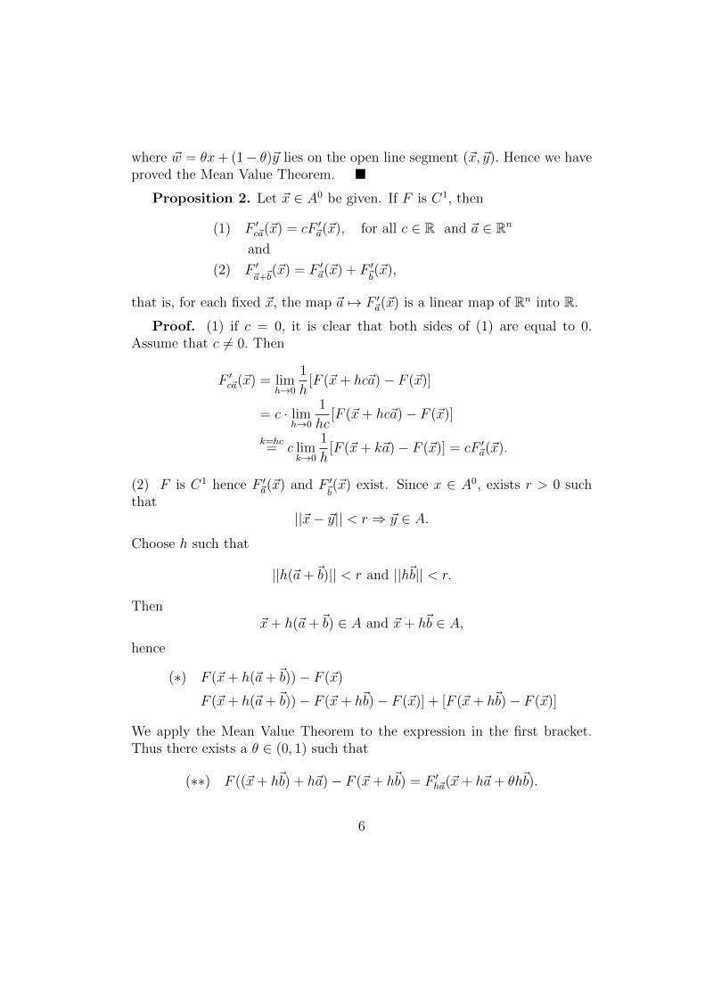
where ~w = θx+ (1− θ)~y lies on the open line segment (~x, ~y). Hence we haveproved the Mean Value Theorem. �
Proposition 2. Let ~x ∈ A0 be given. If F is C1, then
(1) F ′c~a(~x) = cF ′~a(~x), for all c ∈ R and ~a ∈ Rn
and
(2) F ′~a+~b
(~x) = F ′~a(~x) + F ′~b(~x),
that is, for each fixed ~x, the map ~a 7→ F ′~a(~x) is a linear map of Rn into R.
Proof. (1) if c = 0, it is clear that both sides of (1) are equal to 0.Assume that c 6= 0. Then
F ′c~a(~x) = limh→0
1
h[F (~x+ hc~a)− F (~x)]
= c · limh→0
1
hc[F (~x+ hc~a)− F (~x)]
k=hc= c lim
k→0
1
h[F (~x+ k~a)− F (~x)] = cF ′~a(~x).
(2) F is C1 hence F ′~a(~x) and F ′~b(~x) exist. Since x ∈ A0, exists r > 0 suchthat
||~x− ~y|| < r ⇒ ~y ∈ A.
Choose h such that
||h(~a+~b)|| < r and ||h~b|| < r.
Then~x+ h(~a+~b) ∈ A and ~x+ h~b ∈ A,
hence
(∗) F (~x+ h(~a+~b))− F (~x)
F (~x+ h(~a+~b))− F (~x+ h~b)− F (~x)] + [F (~x+ h~b)− F (~x)]
We apply the Mean Value Theorem to the expression in the first bracket.Thus there exists a θ ∈ (0, 1) such that
(∗∗) F ((~x+ h~b) + h~a)− F (~x+ h~b) = F ′h~a(~x+ h~a+ θh~b).
6

By part (1) we have
F ′h~a(~x+ h~a+ θh~b) = hF ′~a(~x+ h~a+ θh~b)
If we divide the equation in (∗∗) by h, then we find
1
h[F ((~x+ h~b) + ~a))− F (~x+ h~b)] = F ′~a(~x+ h~a+ θh~b) −→
h→0F ′~a(~x),
since F is continuously differentiable. Consequently, dividing by h in (∗), itfollows that
limh→0
1
h[F ((~x+ h(~a+~b))− F (~x)]
= F ′~a(~x) + limh→0
1
h[F (~x+ h~b)− F (~x)] = F ′~a(~x) + F ′~b(~x) �
We write ~a =∑n
i=1 ai~ei. Then
F ′~a(~x) =n∑i=1
aiF′~ei
(~x) =n∑i=1
ai∂F
∂xi(~x) = ∇F (~x) · ~a.
As a consequence we have,
Corollary 1. If F is C1 on A ⊆ Rn, then
F ′~a(~x) = ∇F (~x) · ~a,
for all ~x ∈ A0.
If ||~a|| = 1, then F ′~a(~x) is often called the directional derivative of F atthe point ~x in the direction of ~a. From Corollary 1 it follows easily that
Corollary 2. F is continuously differentiable at the point ~x0 ⇔ ∇F iscontinuous at the point ~x0 ⇔ all the first order partial derivatives of F arecontinuous at ~x0.
Proof. Let ~a = (a1, . . . , an) ∈ Rn, ||~a|| = 1. Then
|F ′~a(~x)− F ′~a(~x0)| = |[∇F (~x)−∇F (~x0)] · ~a]|=|∇F (~x)−∇F (~x0)| · ||~a|| · |∇F (~x)−∇F (~x0)|.
This proves that F ′~a(~x) − F ′~a(~x0) −→~x→~x0
0 ⇔ ∇F (~x) − ∇F (~x0) −→~x→~x0
0. Hence
F is continuously differentiable at the point ~x0 ⇔ ∇F is continuous at ~x0.
7
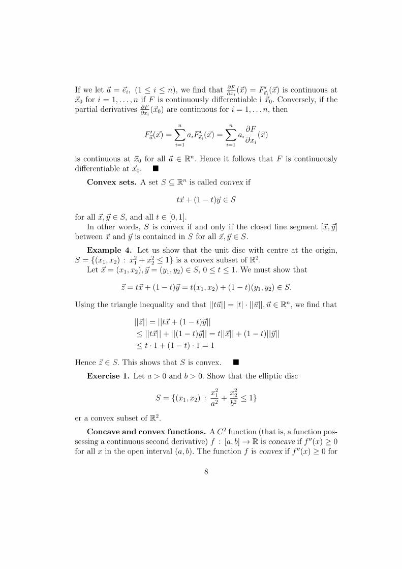
If we let ~a = ~ei, (1 ≤ i ≤ n), we find that ∂F∂xi
(~x) = F ′~ei(~x) is continuous at~x0 for i = 1, . . . , n if F is continuously differentiable i ~x0. Conversely, if thepartial derivatives ∂F
∂xi(~x0) are continuous for i = 1, . . . n, then
F ′~a(~x) =n∑i=1
aiF′~ei
(~x) =n∑i=1
ai∂F
∂xi(~x)
is continuous at ~x0 for all ~a ∈ Rn. Hence it follows that F is continuouslydifferentiable at ~x0. �
Convex sets. A set S ⊆ Rn is called convex if
t~x+ (1− t)~y ∈ S
for all ~x, ~y ∈ S, and all t ∈ [0, 1].In other words, S is convex if and only if the closed line segment [~x, ~y]
between ~x and ~y is contained in S for all ~x, ~y ∈ S.
Example 4. Let us show that the unit disc with centre at the origin,S = {(x1, x2) : x21 + x22 ≤ 1} is a convex subset of R2.
Let ~x = (x1, x2), ~y = (y1, y2) ∈ S, 0 ≤ t ≤ 1. We must show that
~z = t~x+ (1− t)~y = t(x1, x2) + (1− t)(y1, y2) ∈ S.
Using the triangle inequality and that ||t~u|| = |t| · ||~u||, ~u ∈ Rn, we find that
||~z|| = ||t~x+ (1− t)~y||≤ ||t~x||+ ||(1− t)~y|| = t||~x||+ (1− t)||~y||≤ t · 1 + (1− t) · 1 = 1
Hence ~z ∈ S. This shows that S is convex. �
Exercise 1. Let a > 0 and b > 0. Show that the elliptic disc
S = {(x1, x2) :x21a2
+x22b2≤ 1}
er a convex subset of R2.
Concave and convex functions. A C2 function (that is, a function pos-sessing a continuous second derivative) f : [a, b]→ R is concave if f ′′(x) ≥ 0for all x in the open interval (a, b). The function f is convex if f ′′(x) ≥ 0 for
8
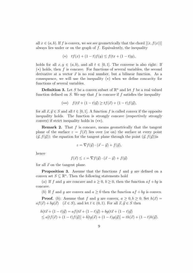
all x ∈ (a, b). If f is convex, we see see geometrically that the chord [(x, f(x))]always lies under or on the graph of f . Equivalently, the inequality
(∗) tf(x) + (1− t)f(y) ≤ f(tx+ (1− t)y),
holds for all x, y ∈ (a, b), and all t ∈ [0, 1]. The converse is also right: If(∗) holds, then f is concave. For functions of several variables, the secondderivative at a vector ~x is no real number, but a bilinear function. As aconsequence, we will use the inequality (∗) when we define concavity forfunctions of several variables.
Definition 3. Let S be a convex subset of Rn and let f be a real valuedfunction defined on S. We say that f is concave if f satisfies the inequality
(∗∗) f(t~x+ (1− t)~y) ≥ tf(~x) + (1− t)f(~y),
for all ~x, ~y ∈ S and all t ∈ [0, 1]. A function f is called convex if the oppositeinequality holds. The function is strongly concave (respectively stronglyconvex) if strict inequality holds in (∗∗).
Remark 2. That f is concave, means geometrically that the tangentplane of the surface z = f(~x) lies over (or on) the surface at every point(~y, f(~y)): the equation for the tangent plane through the point (~y, f(~y))is
z = ∇f(~y) · (~x− ~y) + f(~y),
hencef(~x) ≤ z = ∇f(~y) · (~x− ~y) + f(~y)
for all ~x on the tangent plane.
Proposition 3. Assume that the functions f and g are defined on aconvex set S ⊆ Rn. Then the following statements hold
(a) If f and g are concave and a ≥ 0, b ≥ 0, then the function af + bg isconcave.
(b) If f and g are convex and a ≥ 0 then the function af + bg is convex.
Proof. (b): Assume that f and g are convex, a ≥ 0, b ≥ 0. Set h(~x) =af(~x) + bg(~x) (~x ∈ S), and let t ∈ (0, 1). For all ~x, ~y ∈ S then
h(t~x+ (1− t)~y) = af(t~x+ (1− t)~y) + bg(t~x+ (1− t)~y)
≤ a[tf(~x) + (1− t)f(~y)] + b[tg(~x) + (1− t)g(~y)] = th(~x) + (1− t)h(~y).
9
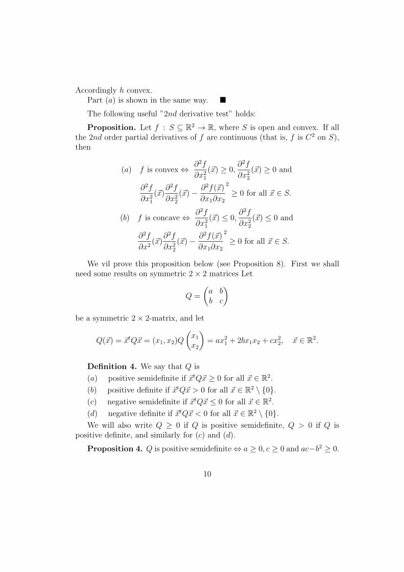
Accordingly h convex.Part (a) is shown in the same way. �
The following useful ”2nd derivative test” holds:
Proposition. Let f : S ⊆ R2 → R, where S is open and convex. If allthe 2nd order partial derivatives of f are continuous (that is, f is C2 on S),then
(a) f is convex⇔ ∂2f
∂x21(~x) ≥ 0,
∂2f
∂x22(~x) ≥ 0 and
∂2f
∂x21(~x)
∂2f
∂x22(~x)− ∂2f(~x)
∂x1∂x2
2
≥ 0 for all ~x ∈ S.
(b) f is concave⇔ ∂2f
∂x21(~x) ≤ 0,
∂2f
∂x22(~x) ≤ 0 and
∂2f
∂x2(~x)
∂2f
∂x22(~x)− ∂2f(~x)
∂x1∂x2
2
≥ 0 for all ~x ∈ S.
We vil prove this proposition below (see Proposition 8). First we shallneed some results on symmetric 2× 2 matrices Let
Q =
(a bb c
)be a symmetric 2× 2-matrix, and let
Q(~x) = ~xtQ~x = (x1, x2)Q
(x1x2
)= ax21 + 2bx1x2 + cx22, ~x ∈ R2.
Definition 4. We say that Q is
(a) positive semidefinite if ~xtQ~x ≥ 0 for all ~x ∈ R2.
(b) positive definite if ~xtQ~x > 0 for all ~x ∈ R2 \ {0}.(c) negative semidefinite if ~xtQ~x ≤ 0 for all ~x ∈ R2.
(d) negative definite if ~xtQ~x < 0 for all ~x ∈ R2 \ {0}.We will also write Q ≥ 0 if Q is positive semidefinite, Q > 0 if Q is
positive definite, and similarly for (c) and (d).
Proposition 4. Q is positive semidefinite⇔ a ≥ 0, c ≥ 0 and ac−b2 ≥ 0.
10

Proof. ⇐: assume that a ≥ 0, c ≥ 0 and ac− b2 ≥ 0. If a = 0 then
ac− b2 = −b2 ≥ 0
hence b = 0. Therefore
(x1, x2)Q
(x1x2
)= (x1, x2)
(0 00 c
)(x1x2
)= (x1, x2)
(0cx2
)= cx22 ≥ 0,
for all (x1, x2). Consequently Q is positive semidefinite.Assume that a 6= 0. Then
(x1, x2)
(a bb c
)(x1x2
)= (x1, x2)
(ax1 + bx2bx1 + cx1
)= ax21 + 2bx1x2 + cx22
= a[x21 + 2b
ax1x2 +
c
ax22]
= a[x21 + 2b
ax1x2 +
b2
a2x22 + (
c
a− b2
a2)x22]
= a[(x1 +b
ax2)
2 +ac− b2
a2x22] ≥ 0
for all (x1, x2) ∈ R2. Hence is Q ≥ 0.
⇒: Assume that Q ≥ 0, then ~xtQ~x ≥ 0, ~x ∈ R2. In particular,
(1, 0)
(a bb c
)(10
)= a ≥ 0
and
(0, 1)
(a bb c
)(01
)= c ≥ 0
Assume that a > 0 : As we have seen above,
(x1, x2)
(a bb c
)(x1x2
)= a[(x1 +
b
ax2)
2 +ac− b2
a2x22].
11

If we let x1 = − bax2, we deduce that ac−b2
a2x22 ≥ 0, for all x2, hence ac−b2 ≥ 0.
Assume that a = 0 : Then
0 ≤ ~xtQ~x = ax21 + 2bx1x2 + cx22= 2bx1x2 + cx22
if b > 0, the fact that x2 = 1, x1 = −n, implies
0 ≤ −2bn+ c −→n→∞
−∞,
yields a contradiction. Hence b = 0, and ac− b2 = 0 ≥ 0. �
Further, it is easy to show
Proposition 5. Q is positive definite⇔ a > 0 (and c > 0) and ac− b2 >0.
Exercise. Prove Proposition 5.
The following chain rule for real functions of several variables will beuseful.
Proposition 6. (Chain Rule) Let f be a real C1- function defined on anopen convex subset S of Rn, and assume that ~r : [a, b]→ S is differentiable.Then the composed function f ◦ ~r = f ◦ (r1, . . . , rn) : [a, b] → R is welldefined. Set g(t) = f(~r(t)). Then g is differentiable and
g′(t) =∂f
∂x1(~r(t))r′1(t) + · · ·+ ∂f
∂xn(~r(t))r′n(t) = ∇f(~r(t)) · ~r ′(t).
Proof. consider
(∗) g(t+ h)− g(t)
h=f(~r(t+ h))− f(~r(t))
h
Since S is open, there exists an open sphere Br with positive radius and centreat ~r(t) which is contained in S. We choose h 6= 0 so small that ~r(t+h) ∈ Br.Set ~u = ~r(t+ h), ~v = ~r(t). Then the numerator on the right hand side of (∗)is f(~u)− f(~v). By applying the Mean Value Theorem to the last difference,we obtain
f(~u)− f(~v) = ∇f(~z) · (~u− ~v),
12

where ~z = ~u + θ(~u− ~v) for a θ ∈ (0, 1). Hence the difference quotient in (∗)may be written
(∗∗) 1
h[g(t+ h)− g(t)] =
1
h∇f(~z) · [(~r(t+ h))− (~r(t))]
As h → 0, we find ~u → ~v, so that ~z → ~u. Sincef is C1, is ∇f continuous,∇f(~z) → ∇f(~u) = ∇f(~r(t)). Therefore the right side of (∗∗) converges to∇f(~r(t)) ·~r ′(t). This shows that g′(t) exists and is equal to the inner product∇f(~r(t)) · ~r ′(t). �
If the function f is defined on an open subset S of R2 for which the partialderivatives of 2nd order exist on S, then we may ask if the two mixed partialderivative are equal. That is, if ∂2f
∂x1∂x2= ∂2f
∂x2∂x1. This is not always the case
however, the following result which we state without proof, will be sufficientfor our needs.
Proposition 7. Assume that f is a real valued function defined on anopen subset S of R2 and that all the first and second order partial derivativesof f are continuouse on S. Then
∂2f
∂x1∂x2(~x) =
∂2f
∂x2∂x1(~x),
for all ~x i S.
Proof. See for instance Tom M. Apostol, Calculus Vol. II, 4.25.
Next we will apply the last four propositions to prove
Proposition 8. Let f be a C2 function defined on an open convex subsetS of R2. Then the following statements hold,
(a) f is convex ⇔ ∂2f∂x21≥ 0, ∂
2f∂x22≥ 0 and ∆f = ∂2f
∂x21
∂2f∂x22− ( ∂2f
∂x1∂x2)2 ≥ 0
(b) f is concave ⇔ ∂2f∂x21≤ 0, ∂
2f∂x22≤ 0 and ∆f ≥ 0
(c) ∂2f∂x21
> 0 and ∆f > 0 ⇒ f is strictly convex.
(d) ∂2f∂x21
< 0 and ∆f > 0 ⇒ f is strictly concave.
Alle the above inequalities are supposed to hold at each point of S.
Proof. (a) ⇐: Choose two arbitrary vectors ~a,~b in S, and let t ∈ [0, 1].We consider the function g given by
g(t) = f(~b+ t(~a−~b)) = f(t~a+ (1− t)~b).
13

Put ~r(t) = ~b+ t(~a−~b), thus g(t) = f(~r(t)). Let ~a = (a1, a2),~b = (b1, b2). TheChain Rule yields
g′(t) = ∇f(~r(t)) · ~r′(t)∂f
∂x1(~r(t)) · (a1 − b1) +
∂f
∂x2(~r(t)) · (a2 − b2)
and
g′′(t) =(∂2f(~r(t))
∂x21,∂2f(~r(t))
∂x2∂x1) · (~a−~b)(a1 − b1)
+ (∂2f(~r(t))
∂x1∂x2,∂2f(~r(t))
∂x22) · (~a−~b)(a2 − b2)
=[∂2f
∂x21(a1 − b1)2 +
∂2f
∂x2∂x1(a1 − b1)(a2 − b2)
+∂2f
∂x1∂x2(a1 − b1)(a2 − b2) +
∂2f
∂x22(a2 − b2)2]~r(t)
=(~a−~b)t(
∂2f∂x21
∂2f∂x1∂x2
∂2f∂x2∂x1
∂2f∂x22
)~r(t)
(~a−~b)
From the conditions in (a) the ”Hessematrix” H of f ,
H =
(∂2f∂x21
∂2f∂x1∂x2
∂2f∂x2∂x1
∂2f∂x22
)
is positive semidefinite in S. Accordingly g′′(t) ≥ 0, for all t ∈ (0, 1), so thatg is convex. In particular it follows that
f(t~a+ (1− t)~b) = g(t) = g(t · 1 + (1− t) · 0)
≤ tg(1) + (1− t)g(0) = tf(~a) + (1− t)f(~b).
Since ~a and ~b were arbitrary in S, we deduce that f is convex.
⇒: In light of Proposition 4 it suffices to prove that the Hessematrix Hof f is positive semidefinite in S. Let ~x ∈ S, h ∈ R2 be arbitrary. As S isopen, there exists r > 0 such that |t| < r ⇒ ~x + t~h ∈ S. Define p on the
interval I = (−r, r) ved p(t) = f(~x+ t~h).
14

Claim: p is a convex function.In order to see this, let λ ∈ [0, 1], t and s ∈ I. Then
p(λt+ (1− λ)s)) = f(~x+ λt~h+ (1− λ)s~h)
= f(λ(~x+ t~h) + (1− λ)(~x+ s~h))
≤ λf(~x+ t~h) + (1− λ)f(~x+ s~h)
= λp(t) + (1− λ)p(s),
which proves the claim.Since p is C2 and convex, we deduce p′′ ≥ 0. Let ~r(t) = ~x+ t~h, t ∈ I. By
The Chain Rule,p′(t) = ∇f(~r(t)) · ~h
and as in the first part of the proof,
p′′(t) = ~htH(~r(t))~h (~h ∈ R2 arbitrary).
As p′′(t) ≥ 0, it follows that H(~r(t)) is positive semidefinite, t ∈ I. In partic-ular,
H(~x) = H(~r(0)) ≥ 0
for all ~x ∈ S. Hence part (a) follows.The proofs of (b), (c) and (d) are similar. �
The following ”gradient inequality” and its consequenses are useful in thecalculus of variations.
Proposition 9. (Gradient inequality) Assume that S ⊆ Rn is convex,and let f : S → R be a C1-function. Then the following equivalence holds
f is concave ⇔
(1) f(~x)− f(~y) ≤ ∇f(~y) · (~x− ~y) =n∑i=1
∂f
∂xi(~y)(xi − yi)
for all ~x, ~y ∈ S.
Proof. ⇒: Assume that f is concave, and let ~x, ~y ∈ S. For all t ∈ (0, 1) :we know that
tf(~x) + (1− t)f(~y) ≤ f(t~x− (1− t)~y),
15

that ist(f(~x)− f(~y)) ≤ f(t(~x− ~y) + ~y)− f(~y)
hence
f(~x)− f(~y) ≤ 1
t[f(~y + t(~x− ~y))− f(~y)]
If we let t → 0, we find that the expression to the right approaches thederivative of f at ~y along ~x− ~y. Hence,
f(~x)− f(~y) ≤ limt→0
1
t[f(~y + t(~x− ~y))− f(~y)] = f ′~x−~y(~y)
= ∇f(~y) · (~x− ~y)
⇐: Assume that the inequality (1) holds. Let ~x, ~y ∈ S, and let t ∈ (0, 1). Weput
~z = t~x+ (1− t)~y.
It is clear that ~z ∈ S, since S is convex. By (1),
(2) f(~x)− f(~z) ≤ ∇f(~z) · (~x− ~z)
and
(3) f(~y)− f(~z) ≤ ∇f(~z) · (~y − ~z)
Multiplying the inequality in (2) by t and the inequality in (3) by 1− t, andthen adding the two resulting inequalities, we derive that
(4) t(f(~x)− f(~z)) + (1− t)(f(~y)− f(~z))
≤ ∇f(~z) · [t(~x− ~z) + (1− t)(~y − ~z)]
Here the right side of (4) equals ~0, since
t(~x− ~z) + (1− t)(~y − ~z) = t~x+ (1− t)~y − t~z − ~z + t~z
= t~x+ (1− t)~y − ~z = ~0.
Rearranging the inequality (4) we hence find,
tf(~x) + (1− t)f(~y) ≤ f(~z) + (1− t)f(~z)
= f(~z) = f(t~x+ (1− t)~y),
which shows that f is convex. �
16
Remark 3. We also have that f is strictly concave ⇔ proper inequalityholds in (1). Corresponding results with the opposite inequality (respectivelythe opposite proper inequality) in (1), holds for convex (respectively stronglyconvex) functions.
Definition 5. Let f : S ⊆ Rn → R, and let ~x∗ = (x∗1, . . . , x∗n) ∈ S.
A vector ~x∗ is called a (global) maximum point for f if f(~x∗) ≥ f(~x) forall ~x ∈ S. Similarly we define global minimum point. ~x∗ is called a localmaximum point for f if there exists a positive r such that f(~x∗) ≥ f(~x) forall ~x ∈ S that satisfies ||~x− ~x∗|| < r.
A stationary (or critical) point for f is a point ~y ∈ S such that∇f(~y) = ~0,that is, all the first order partial derivatives of f at the point ~y are zero,∂f∂xi
(~y) = 0 (1 ≤ i ≤ n).
If ~x∗ is a local maximum- or minimum point in the interior S0 of S, then∇f(~x∗) = ~0 :
∂f
∂xi(~x∗) = lim
h→0+
1
h[f(~x∗)− f(~x∗ + h~ei)] ≥ 0
and∂f
∂xi(~x∗) = lim
h→0−
1
h[f(~x∗)− f(~x∗ + h~ei)] ≤ 0,
and hence ∂f∂xi
(~x∗) = 0, (1 ≤ i ≤ n). For arbitrary C1-functions f the
condition ∇f(~x∗) = ~0 is not sufficient to ensure that f has a loal maximumor minimum at ~x∗, however, if f is convex or concave, the following holds,
Proposition 10. Let f be a real valued C1 function defined on a convexsubset S of Rn, and let ~x∗ ∈ S. The following holds
(a) if f is concave, then ~x∗is a local maximum point for f
⇔ ∇f(~x∗) = ~0.
(b) if f is convex, is ~x∗ a local minimum point for f
⇔ ∇f(~x∗) = ~0.
Proof. (a)⇒: We have seen above that if ~x∗ is a local maximum point for f , then∇f(~x∗) = ~0.
17
⇐: Assume that ~x∗ is a stationary point and that f is concave. For all ~x ∈ Sit follows from the gradient inequality in Proposition 9 that
f(~x)− f(~x∗) ≤ ∇f(~x∗) · (~x− ~x∗) = 0,
hence f(~x) ≤ f(~x∗), for all ~x ∈ S.the proof of (b) is similar.
The next result will also be useful,
Proposition 11. Assume that F is a real valued function defined on aconvex subset S of Rn, and that G is a real function defined on an interval inR that contains the image f(S) = {f(~x) : ~x ∈ S} of f . Then the followingstatements hold,
(a) f is concave and G is concave and increasing ⇒ G ◦ f is concave.
(b) f is convex and G is convex and increasing ⇒ G ◦ f is convex.
(c) f is concave and G is convex and decreasing ⇒ G ◦ f is convex.
(d) f is convex and G concave and decreasing ⇒ G ◦ f is concave.
Proof. (a) Let ~x, ~y ∈ S, and let t ∈ (0, 1). Put U = G ◦ f. Then
U(t~x+ (1− t)~y) = G(f(t~x+ (1− t)~y)
≥ G(tf(~x) + (1− t)f(~y)) (f concave and G increasing)
≥ tG(f(~x)) + (1− t)G(f(~y)) (G concave)
= tU(~x) + (1− t)U(~y),
hence U is concave.(b) is proved as (a).(c) and (d): Apply (a) and (b) to the function −G. (Notice that G is convexand decreasing ⇔ −G is concave and increasing.) �
3 CALCULUS OF VARIATIONS.
We may say that the basic problem of the calculus of variations is to deter-mine the maximum or minimum of an integral of the form
(1) J(x) =
∫ t1
t0
F (t, x(t), x(t)) dt,
18

where F is a given C2 function of three variables and x = x(t) is an unknownC2 function on the interval [t0, t1], such that
(2) x(t0) = x0, and x(t1) = x1,
where x0 and x1 are given numbers. Additional side conditions for the prob-lem may also be included. Functions x that are C2 and satisfy the endpointconditions (2) are called admissible functions.
Example 1. (Minimal surface of revolution.)Consider curves x = x(t) in the tx−plane, t0 ≤ t ≤ t1, all with the samegiven, end points (t0, x0), (t1, x1). By revolving such curves around the t−axis,we obtain a surface of revolution S.Problem. Which curve x gives the smallest surface of revolution?If we assume that x(t) ≥ 0, the area of S is
A(x) =
∫ t1
t0
2πx√
1 + x2 dt
Our problem is to determine the curve(s) x∗ for which minA(x) = A(x∗),when x(t0) = x0, x(t1) = x1. This problem is of the same type as in (1)above.
We shall next formulate the main result for problems of the type (1).
Theorem 1. (”Main Theorem of the Calculus of Variations”)Assume that F is a C2 function defined on R3. Consider the integral
(∗)∫ t1
t0
F (t, x, x) dt
If a function x∗ maximizes or minimizes the integral in (∗) among all C2
functions x on [t0, t1] that satisfy the end point conditions
x(t0) = x0, x(t1) = x1,
then x∗ satisfies the Euler equation
(E)∂F
∂x(t, x(t), x(t))− d
dt(∂F
∂x(t, x(t), x(t)) = 0 (t ∈ [t0, t1]).
If the function (x, x) 7→ F (t, x, x) is concave (respectively convex) for eacht ∈ [t0, t1], then a function x∗ that satisfies the Euler equation (E), solvesthe maximum (respectively minimum) problem.
19

Solutions of the Euler equations are called stationary points or ex-tremals. A proof of Theorem 1 will be given below. First we consider anexample.
Example 2. Solve
minx
∫ 1
0
(x2 + x2) dt, x(0) = 0, x(1) = e2 − 1.
We let F (t, x, x) = x2 + x2. Then ∂F∂x
= 2x, ddt∂F∂x
= ddt
(2x) = 2x. Hence theEuler equation of the problem is
x− x = 0,
The general solution isx(t) = Aet +Be−t
Here x(0) = 0 = A+ B,B = −A, x(1) = e2 − 1 = Ae+ Be−1 = A(e− e−1).This implies that A = e, B = −e, hence
x(t) = et+1 − e1−t
is the only possible solution, by the first part of Theorem 1. Here F (t, x, x) =x2 + x2 is convex as a function of (x, x), for each t (this follows from the 2ndderivative test, or from the fact that F is a sum of two convex functions eachof them of a single variable: x 7→ x2, and x 7→ x2). As a consequence of thelast part of Theorem 1, we conclude that x does in fact solve the problem.The minimum is∫ 1
0
(x2 + x2) dt =
∫ 1
0
[(et+1 − e1−t)2 + (et+1 + e1−t)2] dt = . . . = e4 − 1.
We notice that t does not occur explicitly in the formula for F in this example.Next we shall take a closer look at this particular case.
The case F = F (x, x) (that is, t does not occur explicitly in the formulaof the function F ). Such problems are often called autonomous.
If x(t) is a solution of the Euler equation, then the Chain Rule yields:
d
dt[f(x, x)− x∂F
∂x(x, x)] =
∂F
∂xx+
∂F
∂xx− x∂F
∂x− x d
dt
∂F
∂x
= x[∂F
∂x− d
dt(∂F
∂x)] = x · 0 = 0,
20
so that
F − x∂F∂x
= C (is constant).
This equation is called a first integral of the Euler equation.
In order to prove Theorem 1 we will need,
The Fundamental Lemma (of the Calculus of Variations). Assumethat f : [t0, t1]→ R is a continuous function, and that∫ t1
t0
f(t)µ(t) dt = 0
for all C2 functions µ that satisfies µ(t0) = µ(t1) = 0. Then f(t) = 0 for allt in the interval [t0, t1].
Proof. If there exists an s ∈ (t0, t1) such that f(s) 6= 0, say f(s) > 0,then f(t) > 0 for all t in some interval [s− ε, s+ ε] of s since f is continuous.We choose a function µ such that µ is C2 and
µ ≥ 0, µ(s− ε) = µ(s+ ε) = 0, µ > 0 on (s− ε, s+ ε),
and µ = 0 outside the interval (s− ε, s+ ε). We may for instance let{(t− (s− ε))3((s+ ε)− t)3, y ∈ [s− ε, s+ ε]
0, t /∈ [s− ε, s+ ε].
which is C2. Then∫ t1
t0
f(t)µ(t) dt =
∫ s+ε
s−εf(t)µ(t) dt > 0.
since µ(t)f(t) > 0 and µ(t)f(t) is continuous on the open interval (s−ε, s+ε).Hence we have obtained a contradiction. �
We shall also need to ”differentiate under the integral sign”:
Proposition 2. Let g be a C2 function defined on the rectangle R =[a, b]× [c, d] i R2, and let
G(u) =
∫ b
a
g(t, u) dt, u ∈ [c, d].
21

Then
G′(u) =
∫ b
a
∂g
∂u(t, u) dt.
Proof. Let ε > 0. Since ∂g∂u
is continuous, it is also uniformly continuous onR (R is closed and bounded, hence compact). Therefore there exists a δ > 0such that
|∂g∂u
(s, u)− ∂g
∂u(t, v)| < ε
b− a,
for all (s, u), (t, v) in R such that ||(s, u) − (t, v)|| < δ. By the Mean valueTheorem there is a θ = θ(t, u, v) between u and v such that
g(t, v)− g(t, u) =∂g
∂u(t, θ)(v − u).
Consequently,
|∫ b
a
[g(t, v)− g(t, u)
v − u− ∂g
∂u(t, u)] dt|
≤∫ b
a
|∂g∂u
(t, θ)− ∂g
∂u(t, u)| dt
≤∫ b
a
ε
b− adt = ε, for |v − u| < δ.
Hence
G′(u) = limv→u
G(v)−G(u)
v − u= lim
v→u
∫ b
a
g(t, v)− g(t, u)
v − udt
=
∫ b
a
∂g
∂u(t, u) dt.
�
Proof of Theorem 1. We will consider the maximum problem (theminimum problem is similar)
(1)
maxx
∫ t1
t0
F (t, x(t), x(t)) dt
when x(t0) = x0 and x(t1) = x1, (here x0, and x1 are given numbers.
22
assume that x∗ is a C2 function that solves (1). Let µ be an arbitrary C2
function on [t0, t1] that satisfies µ(t0) = µ(t1) = 0. For each real ε the function
x = x∗ + εµ
is an admissible function, that is, a C2 function satisfying the endpoint con-ditions x(t0) = x0 and x(t1) = x1. Therefore we must have
J(x∗) ≥ J(x+ εµ)
for all real ε. Let µ be fixed. We will study I(ε) = J(x∗ + εµ) as a functionof ε. The function I has a maximum for ε = 0. Hence
I ′(0) = 0.
Now
I(ε) =
∫ t1
t0
F (t, x∗(t) + εµ(t), x∗(t) + εµ(t)) dt
Differentiating under the integral sign (see Proposition 2 above) with respectto ε we find by the Chain Rule,
0 = I ′(0) =
∫ t1
t0
[∂F ∗∂x
µ(t) +∂F ∗
∂xµ(t)
]dt
where we put ∂F ∗
∂x= ∂F
∂x(t, x∗(t), x∗(t)) and ∂F ∗
∂x= ∂F ∗
∂x(t, x∗(t), x∗(t)). Hence
0 = I ′(0) =
∫ t1
t0
∂F ∗
∂xµ(t) dt+
∫ t1
t0
∂F ∗
∂xµ(t) dt
=
∫ t1
t0
∂F ∗
∂xµ(t) dt+
[∂F ∗
∂xµ(t)
]t1t0
−∫ t1
t0
d
dt
(∂F ∗∂x
)µ(t) dt (using integration by parts)
=
∫ t1
t0
[∂F ∗∂x− d
dt
(∂F ∗∂x
)]µ(t) dt (since µ(t1) = µ(t0) = 0)
hence ∫ t1
t0
[∂F ∗∂x− d
dt
(∂F ∗∂x
)]µ(t) dt = 0
for all such C2 functions µ with µ(t1) = µ(t1) = 0. By the FundamentalLemma it follows that
(2)∂F ∗
∂x− d
dt
(∂F ∗∂x
)= 0,
23

hence x∗ satisfies the Euler equation. Using a quite similar argument we findthat an optimal solution x∗ for the minimum problem also satisfies (2).
Sufficiency: assume that for every t in [t0, t1], F (t, x, x) is concave withrespect to the last two variables (x, x), and let x∗ satisfy the Euler equationwith the endpoint conditions of (1). We shall prove that x∗ solves the max-imum problem. Let x be an arbitrary admissible function for the problem.By concavity the ”Gradient inequality” yields,
F (t, x, x)− F (t, x∗, x∗) ≤ ∂F ∗
∂x(x− x∗) +
∂F ∗
∂x(x− x∗)
d
dt(∂F ∗
∂x)(x− x∗) +
∂F ∗
∂x(x− x∗) =
d
dt(∂F ∗
∂x(x− x∗)),
for all t ∈ [t0, t1]. By integration of the inequality we deduce that∫ t1
t0
(F (t, x, x)− F (t, x∗, x∗)
)dt
≤∫ t1
t0
d
dt
( ∂F ∗∂x
)(x− x∗) dt =
[∂F ∗
∂x(x− x∗)
]t1t0
= 0,
where we used the endpoint conditions for x and x∗ at the last step. Hence∫ t1
t0
F (t, x, x) dt ≤∫ t1
t0
F (t, x∗, x∗) dt
as we wanted to prove. �
Remark. In the above theorem, assume instead that F is concave withrespect to (x, x) (for each t ∈ [t0, t1]) only in a certain open and convexsubset R of R2. The above sufficiency proof still applies to the set V ofall admissible functions x enjoying the property that (x(t), x(t)) ∈ R for allt ∈ [t0, t1]. Hence any admissible solution x∗ of the Euler equation that isalso an element of V will maximize the integral
∫ t1t0F (t, x, x) dt among all
members of V . Consequently, we obtain a maximum relative to the set V .Note that the proof uses the ”Gradient Inequality” (Proposition 9 in Section1) which requires the region to be open and convex.
Example 3. We will find a solution x = x(t) of the problem
min
∫ 1
−1F (t, x, x) dt
24

where F (t, x, x) = t2x2 + 12x2 and x(−1) = −1, x(1) = 1.
(a) First we will solve the problem by means of Theorem 1. Here we find
∂F
∂x− d
dt
(∂F∂x
)= 24x− d
dt
(t2 · 2x
)= 24x− 4tx− 2t2x,
and the Euler equation takes the form
t2x+ 2tx− 12x = 0.
We seek solutions of the type x(t) = tk. This gives
(k(k − 1) + 2k − 12)tk = 0, for all t,
that is, k2 + k − 12 = 0, which has the solutions k = 3 and k = −4.Consequently, x(t) = At3 +Bt−4 where
x(−1) = −A+B = −1
x(1) = A+B = 1
Hence B = 0 and A = 1, so that x(t) = t3 is the only possible solution.Furthermore,
∂2F
∂x2= 2t2 ≥ 0,
∂2F
∂x2= 24 > 0,
∂2F
∂x∂x= 0,
and the determinant of the Hesse matrix is 24 ·2t2 = 48t2 ≥ 0. It follows thatF is convex with respect to (x, x). Hence, in view of Theorem 1, x(t) = t3
gives a minimum. �
(b) Suppose next that x is a solution of the Euler equation to the problemwhich in addition satisfies the given endpoint conditions. If z is an arbitraryadmissible function, then µ = z − x is a C2 function that satisfies µ(−1) =µ(1) = 0. Let us show that
J(z)− J(x) = J(x+ µ)− J(x) ≥ 0.
From this it will follow that x minimizes J . Now
J(x+ µ)− J(x) =
∫ 1
−1[t2(x+ µ)2 + 12(x+ µ)2 − t2x2 − 12x2] dt
=
∫ 1
−1[2t2xµ+ t2µ2 + 24xµ+ 12µ2] dt =
∫ 1
−1[t2µ2 + 12µ2] dt+ I
25
where
I =
∫ 1
−1[2t2xµ+ 24xµ] dt
=
∣∣∣∣1−1
2t2xµ−∫ 1
−1(2t2xµ+ 4txµ) dt+
∫ 1
−124xµ dt (using integration by parts)
= 0−∫ 1
−12µ[t2x+ 2tx− 12x] dt
(µ(−1) = µ(1) = 0
)= 0,
where the last inequality follows from the fact that x satisfies the Eulerequation
t2x+ 2tx− 12x = 0.
Hence
J(x+ µ)− J(x) =
∫ 1
−1[t2µ2 + 12µ2] dt > 0
if µ 6= 0, hence every solution of the Euler equation that satisfies the endpointconditions, yields a minimum. We have seen in (a) that x(t) = t3 is the onlysuch solution. �
Example 4. (No minimum)Consider the minimum problem
min
∫ 4
0
(x(t)2 − x(t)2) dt, x(0) = 0, x(4) = 0.
The Euler equation(E) x+ x = 0
has the characteristic roots ±i, hence the general solution of (E) is
x(t) = A cos t+B sin t
The endpoint conditions yield A = B = 0, hence the unique solution is
x∗(t) = 0 (for all t ∈ [0, 4])
Consequently, if the minimum exists, then it is equal to zero and is attainedat x∗ = 0. Let us show that the minimum does not exist. To that end, weconsider the function
x(t) = sin(πt
4)
26
which is clearly C2. Moreover, x(0) = x(4) = 0, so that x is admissible. Now∫ 4
0
(x2 − x2) dt =
∫ 4
0
[π2
16cos2(
πt
4)− sin2(
πt
4)] dt
=
∫ 4
0
(π2
16− (
π2
16+ 1) sin2 πt
4) dt =
π2
4− (
π2
16+ 1)
∫ 4
0
1
2(1− cos
πt
2) dt
=π2
4− (
π2
16+ 1)
1
2
[40t− 2
πsin
πt
2
]=π2
4− (
π2
16+ 1)
1
2[4− 0] = −π
2
8− 2 < 0
Therefore, x∗ = 0 does not minimize the integral and no minimum exists.
Other endpoint conditions. Next we will consider optimation prob-lems for which the left end point x(t0) of the admissible functions x is fixed,whereas the right end point x(t1) is free. In this case we have the followingresult:
Theorem 2. Assume that x0 is a given number. A necessary conditionfor a C2 function2 x∗ to solve the problem
max (min)
∫ t1
t0
F (t, x(t), x(t)) dt, x(t0) = x0, x(t1) is free,
is that x∗ satisfies the Euler equation and, in addition, the condition
(T )(∂F∂x
)t=t1
= 0.
If the function F (t, x, x) is concave (respectively convex) in (x, x) for eacht ∈ [t0, t1], then any admissible function x∗ that satisfies the Euler equationand the condition (T ), solves the maximum (respectively minimum) problem.
The condition (T ) is called the transversality condition.
Proof. We will give a proof of the maximum problem. The proof ofthe minimum problem is similar. Assume that x∗ solves the problem. Inparticular all admissible (C2) functions x which have the same value x∗(t1)as x∗ at the right endpoint t = t1, satisfy J(x) ≤ J(x∗), hence x∗ is optimalamong those functions. However, then x∗ satisfies the Euler equation. In the
2As can be shown, it suffices to consider C1-functions. In fact, even piecewise C1-functions will do.
27

proof of the Euler equation, see the proof of Theorem 1, we considered thefunction
I(α) =
∫ t1
t0
F (t, x∗ + αµ, x∗ + αµ) dt
After integration by parts and differentiation under the integral, we con-cluded that
0 = I ′(0) =
∫ t1
t0
[∂F ∗
∂x− d
dt(∂F ∗
∂x)] dt+
[ ∂F ∗∂x
µ(t)]t1t0,
where
(∗) ∂F ∗
∂x=∂F
∂x(t, x∗(t), x∗(t)) and
∂F ∗
∂x=∂F
∂x(t, x∗(t), x∗(t))
Here, at this point, we let µ be a C2 function such that µ(t0) = 0 and µ(t1) isfree. Since x∗ satisfies the Euler equation, the integral in (∗) must be equalto zero, hence
µ(t1)( ∂F ∗∂x
)t=t1
= 0.
If we choose a µ with µ(t1) 6= 0, it follows that ( ∂F∗
∂x)t=t1 = 0.
Sufficiency: Assume that F (t, x, x) is concave in (x, x), and that x∗ isan admissible function which satisfies the Euler equation and the condition(T ). The argument led to the inequality∫ t1
t0
(F (t, x, x)− F (t, x∗, x∗)
)dt
≤∫ t1
t0
d
dt
( ∂F ∗∂x
)(x− x∗) dt =
[∂F ∗
∂x(x− x∗)
]t1t0
The last part of the proof of Theorem 1, goes through as before. Here wefind [
∂F ∗
∂x(x− x∗)
]t=t0
= 0
since x(t0) = x∗(t0) = x0. Finally the condition (T ) yields[∂F ∗
∂x(x− x∗)
]t=t1
= 0.
28
Thus it follows that J(x) ≤ J(x∗), hence x∗ maximizes J. �
Using techniques similar to those of the previous proof, we can show
Theorem 3.Assume that t0, t1, x0, and x1 are given numbers, and let F be a C2 functiondefined on R3. Consider the integral
(∗)∫ t1
t0
F (t, x(t), x(t)) dt
If a function x∗ maximizes or minimizes the integral in (∗) among all C2
functions x on [t0, t1] that satisfy the end point conditions
x(t0) = x0, x(t1) ≥ x1,
then x∗ satisfies the Euler equation
(E)∂F
∂x(t, x(t), x(t))− d
dt(∂F
∂x(t, x(t), x(t)) = 0 (t ∈ [t0, t1]).
and the transversality condition
(T )(∂F∂x
)t=t1≤ 0 (= 0 if x(t1) > x1).
If the function (x, x) 7→ F (t, x, x) is concave (respectively convex) foreach t ∈ [t0, t1], then a function x∗ that satisfies the Euler equation (E),solves the maximum (respectively minimum) problem.
Exercise 1. Let
F (t, x, x) = x2 + 7xx+ x2 + tx
(a) Find the Euler equation (E) of the function F . Is F concave orconvex as a function of the last two variables (x, x) ?
(b) Find the general solution of (E).(c) Express the integral ∫ t1
t0
x(t)x(t) dt
29

as a function of x(t0) and x(t1). Find a solution x of the problem
min
∫ 1
0
F (t, x(t), x(t)) dt, x(0) =1
2, x(1) =
3
2
Exercise 2. Find a function F (t, x, x) which has the given differentialequation as an Euler equation:
(a)x− x = 0
(b)t2x+ 2tx− x = 0
(c) Decide if the functions F of (a) and (b) are concave or convex asfunctions of (x, x) for fixed t.
(d) Find the only C2−function x∗ of the variation problem
min
∫ 1
0
(1
2x2 +
1
2x2)
dt, x(0) = 0, x(1) = e− e−1,
Justify your answer.(e) Let F be as in (b) and solve the problem
min
∫ π√3
0
F (t, x(t), x(t)) dt, x(0) = 1, x(π√3
) = 2e−π2√3 .
Exercise 3. Consider the problem min J(x), where
J(x) =
∫ 2
1
x(1 + t2x) dt, x(1) = 3, x(2) = 5.
(a) Find the Euler equation of the problem and show that it has exactlyone solution x that satisfies the given endpoint conditions.
(b) Apply Theorem 1 to prove that the solution from (a) really solvesthe minimum problem.
(c) For an arbitrary C2 function µ that satisfies µ(1) = µ(2) = 0, showthat
J(x+ µ)− J(x) =
∫ 2
1
t2µ2 dt,
30

where x is the solution from (a). Explain in light of this, that x minimizesJ .
Exercise 4. A function F is given by
F (x, y) = x2(1 + y2), (x, y) ∈ R2
(a) Show that F is convex in the region
R = {(x, y) : |y| ≤ 1√3}
(b) Show that the variation problem
min
∫ 1
0
x2(1 + x2) dt,
x(0) = x(1) = 1
has Euler equation
(∗) xx+ x2 − 1 = 0
(c) Find the only possible solution x∗ of the variation problem. Let
V = {x : x is a C2 function such that x(0) = x(1) = 1
and |x(t)| < 1√3
for all t ∈ [0, 1]}
Show that x∗ ∈ V . Explain that x∗ minimizes the integral in (1) among allfunctions in V .
Exercise 5. (Reduction of order)Suppose that one solution x1 of the homogeneous linear differential equation
(∗) x+ p(t)x+ q(t)x = 0
is known on an interval I where p and q are continuous. Substitute
x2(t) = u(t)x1(t)
into the equation (∗) to deduce that x2 is a solution of (∗) if
(∗∗) x1u+ (2x1 + px1)u = 0
31
Since (∗∗) is a separable first order equation in v = u, it is readily solved forthe derivative u of u and hence for u. This is called the method of reductionof order. As u is nonconstant, the general solution of (∗) is
x = c1x1 + c2x2 (c1, c2 arbitrary constants).
Exercise 6. Let α > −1, and put
(∗) F (t, x, x) =1
2(1− t2)x2 − 1
2α(α + 1)x2 + tx+
1
2t2x
(a) Show that the Euler equation of F is
(∗∗) (1− t2)x− 2tx+ α(α + 1)x = 0
This is known as the Legendre equation of order α and is important in manyapplications.
(b) Let α = 1 in (∗∗). Show that in this case the function x1(t) = t isa solution of the equation (∗∗). Then use the method of reduction of order(Exercise 5) to derive the second solution
x2(t) = 1− 1
2t ln |1 + t
1− t|, for t 6= ±1.
(c) Find all possible C2−solutions of the variation problem
max
∫ 3
2
F (t, x, x) dt, x(2) = 0, x(3) =3
2ln
3
2− 1
2.
(d) Find the optimal x of the problem in (c)
Exercise 7. Find the unique C2− solution x of the minimum problem
min
∫ e
1
(x2 + txx+ t2x2) dt, x(1) = 0, x(e) = er1 − er2 ,
where r1 = 12(−1 +
√3) and r2 = 1
2(−1−
√3)
Exercise 8. Let
F (t, x, x) = x2 +1
2t(t− 1)x2,
32

and consider the problem
(1) min
∫ 3
2
F (t, x(t), x(t)) dt, x(2) = 0, x(3) = ln25
27.
(a) Find the Euler equation (E) of the problem in (1).(b) Show that (E) has a polynomial solution x1.(c) Use reduction of order (see Exercise 5) to find another solution x2 of
(E) such that x2(t) = v(t)x1(t), t ∈ [2, 3].(d) What is the general solution of (E) ? Find the only solution x∗ of
(E) that satisfies the endpoint conditions in (1).(e) Decide if x∗ minimizes the integral in (1).Remark. The Euler equation (E) of Exercise 8 (a) is a special case of
Gauss’ hypergeometric differential equation
(G) t(1− t)x+ [c− (a+ b+ 1)t]x− abx = 0
where a, b, and c are constants. Hypergeometric differential equations occurfrequently in both mathematics and physics. In particular, they are obtainedfrom certain interesting partial differential equations by separation of vari-ables.
Exercise 9. In the followig we shall study maxima and minima of
(∗) J(x) =
∫ 2
1
F (t, x(t), x(t)) dt, x(1) = −1
3, x(2) is free .
Here
F (t, x, x) =1
2x2 +
1
6g(t)x3,
and g is a positive (g > 0) C2−function on [1, 2].(a) Find the Euler equation (E) of the problem. Express x in terms of
g.From now on we let
g(t) =1
t2, for all t ∈ [1, 2].
(b) Find the general solution of (E) in this special case.(c) Show that (E) has exactly two solutions x1 and x2 which satisfy the
endpoint conditions of (∗).
33

(d) Consider the two following convex sets of functions,
R1 = {x : x ∈ C2[1, 2], x(1) = −1
3, x(2) is free, x(t) > −1 (for all t ∈ [1, 2])}
and
R2 = {x : x ∈ C2[1, 2], x(1) = −1
3, x(2) is free, x(t) < −1 (for all t ∈ [1, 2])}
Decide if the function (x, x) 7→ F (t, x, x) (t ∈ [1, 2] arbitrary, fixed) is con-cave or convex on R1 or on R2. Does J(x) have a maximum or a minimumon any of the two sets R1, R2 ? Find the maximum and the minimum of J(x)on R1 and on R2 if they exist.
Remark. The Euler equation of Exercis 9 (a) (with y = x) is a simplespecial case of an Abel differential equation of the 2nd kind:
(1) (y + s)y + (p+ qy + ry2) = 0,
where p, q, r, and s are C1−functions of a real variable on an open intervalI. Such equations can always be reduced to the simpler form
(2) zz + (P +Qz) = 0
via a substitution y = α + βz, where α and β are C1−functions on I. Infact, we may let
α = −s, β(t) = e−∫r(t) dt, P = (p−qs+rs2)e2
∫r(t) dt, Q = (q−2rs− s)e
∫r(t) dt.
The simple special case (E) of Exercise 9 (a) may be solved without such a re-duction. Abel studied equation (1) in the 1820-s and he made the mentionedreduction to (2). (Œuvres completes de Niels Henrik Abel, Tome Second, p.26-35.)
Weierstrass’ sufficiency condition.3
Example 5. Consider the problem of maximizing or minimizing theintegral
J(x) =
∫ 1
0
(x2 − x2) dt, x(0) = x(1) = 0.
3This section is optional.
34
The Euler equation of the problem is
x+ x = 0
The extremals (that is, the solutions of the Euler equation) are
x(t) = A sin t+B cos t, A and B arbitrary constants.
Among all extremals only the zero function x∗, x∗(t) = 0 for all t ∈ [0, 1],satisfies the endpoint conditions. It is easy to see, using the second-derivativetest, that F (t, x, x) = x2 − x2 is neither concave nor convex i (x, x). Hencewe cannot use Theorem 1 to decide if x∗ gives a maximum or a minimum forthe problem.
Exercise 10. Show that the function F (t, x, x) = x2 − x2 of the lastExample is neither convex nor concave.
The sufficiency condition stated in Theorem 3 below, is often useful forsolving problems of the type
(1) max or min J(x)
where
J(x) =
∫ t1
t0
F (t, x(t), x(t)) dt.
As above F is assumed to be a given C2 function of three variables andx = x(t) is an unknown C2 function on the interval [t0, t1], such that
(2) x(t0) = x0, x(t1) = x1,
where x0 and x1 are given numbers.The solutions of the Euler equation of this problem (without any endpoint
conditions), are called extremals.
Definition. we say that an extremal x∗ for
J(x) =
∫ t1
t0
F (t, x(t), x(t)) dt, x(t0) = x0, x(t1) = x1,
is a relative maximum if there exists an r > 0 such that J(x∗) ≥ J(x) for allC2 functions x with x(t0) = x0, x(t1) = x1 that satisfies |x∗(t)−x(t)| < r forall t ∈ [0, 1]. A relative minimum x∗ is defined similarly.
35

Theorem 4. (Weierstrass’ sufficiency condition). Assume that an ex-tremal x∗ for the problem (1) satisfies the endpoint conditions (2) and thatthere exists a parameter family x(·, α) 4, −ε < α < ε, of extremals such that
(1) x(t, 0) = x∗(t), t ∈ [t0, t1],
(2) x(·, α) is differentiable with respect to α and∂x
∂α(t, α)
∣∣α=06= 0,
t0 ≤ t ≤ t1,
(3) if α1 6= α2, then the two curves given by x(·, α1) and x(·, α2)have no
common points,
(4)∂2F
∂x2(t, x, x) < 0 for all t ∈ [t0, t1] and all x = x(·, α), α ∈ (−ε, ε)
Then x∗ is a relative maximum for J(x) with the given endpoint conditions.If the condition
(4′)∂2F
∂x2(t, x, x) > 0 for all t ∈ [t0, t1] and all x = x(·, α), α ∈ (−ε, ε),
holds instead of (4), then x∗ is a relative minimum.
Example 6. Consider the extremals
x(t) = A cos t+B sin t, t ∈ [0, 1].
of Example 5. The parameter family of extremals x(·, α) given by
(∗) x(t, α) = α cos t, α ∈ (−1, 1),
satisfies x(·, 0) = x∗ = 0, and is differentiable with respect to α with∂x(t,α)∂α
∣∣α=0
= cos t 6= 0 for all t ∈ [0, 1]. Moreover, it is clear that the familyof curves given by (∗) have no common points. Finally we have
∂2F
∂x2(t, x, x) =
∂
∂x(2x) = 2 > 0.
Hence, by the Weierstrass sufficiency condition, x∗ = 0 is a relative minimumpoint for J(x).
4For fixed α, x(·, α) denotes the function t 7→ x(t, α)
36
Exercise 11. Let
J(x) =
∫ t1
t0
√1 + x2 dt, x(t0) = x0, x(t1) = x1, where t0 6= t1.
J(x) gives the arc length of the curve x(t) between the two given points(t0, x0) and (t1, x1). We wish to determine the curve x∗ that yields theminimal arc length.
(a) Show that the Euler equation of the problem may be written
(E)x√
1 + x= c, where c is a constant different from ± 1.
(b) Show that (E) has a unique solution x∗ that satisfies the givenendpoint conditions.
(c) Show that among the solutions of (E) there exists a parameter familygiven by x(t, α) = x∗(t) +α, −1 < α < 1, where x∗ is as in (b), and that theconditions of Theorem 3 are satified such that x∗ gives a (relative) minimum.
(d) Show that F (t, x, x) is convex i (x, x). Conclude by Theorem 1 thatx∗ solves the minimum problem.
Exercise 12.(a) Verify that x1(t) = t−1 cos t is a solution of
(∗) tx+ 2x+ tx = 0, (t 6= 0).
(b) Find another solution x2 of the equation in (∗) of the form
x2 = ux1,
using reduction of order (see Exercise 5).Next let
F (t, x, x) =1
2t2x2 +
1
3t3xx,
and consider the problem
(∗∗) min
∫ π2
π6
F (t, x, x) dt, x(π
6) = 0, x(
π
2) = 1.
(c) Write down the Euler equation of (∗∗) and find its general solution.(d) Find the only possible solution x∗ of the variation problem in (∗∗)
and decide if x∗ is optimal.
37
4 OPTIMAL CONTROL THEORY.
In the Calculus of Variations we studied problems of the type
max/min
∫ t1
t0
f(t, x(t), x(t)) dt, x(t0) = x0, x(t1) = x1 (or x(t1) free).
We assumed that all the relevant functions were of class C2 (twice continu-ously differentiable). If we let
u = x,
then the above problem may be reformulated as
(0) max/min
∫ t1
t0
f(t, x(t), u(t)) dt, x = u, x(t0) = x0, x(t1) = x1(or x(t1) free).
We shall next study a more general class of problems, problems of the type:
(1)
max/min
∫ t1t0f(t, x(t), u(t)) dt, x(t) = g(t, x(t), u(t)),
x(t0) = x0, x(t1) free,
u(t) ∈ R, t ∈ [t0, t1], u piecewise continuous.
Later we shall also consider such problems with other endpoint conditionsand where the functions u can take values in more general subsets of R.
Such problems are called control problems, u is called a control vari-able (or just a control). The control region is the common range of thepossible controls u.5 Pairs of functions (x, u) that satisfies the given end-point conditions and, in addition, the equation of state x = g(t, x, u), arecalled admissible pairs.
We shall always assume that the controls u are piecewise continuous, thatis, u may possess a finite number of jump discontinuities. (In more advancedtexts measurable controls are considered.) In the calculus of variations wealways assumed that u = x was of class C1.
In the optimal control theory it proves very useful to apply an auxiliaryfunction H of four variables defined by
H(t, x, u, p) = f(t, x, u) + pg(t, x.u),
called the Hamilton function or Hamiltonian of the given problem.
5Variable control regions may also be considered
38
Pontryagin’s Maximum principle gives conditions that are necessary foran admissible pair (x∗, u∗) to solve a given control problem:
Theorem (The Maximum Principle I)
Assume that (x∗, u∗) is an optimal pair for the problem in (1). Thenthere exist a continuous function p = p(t), such that for all t ∈ [t0, t1], thefollowing conditions are satisfied:
(a) u∗(t) maximizes H(t, x∗(t), u, p(t)), u ∈ R, that is,
H(t, x∗(t), u, p(t)) ≤ H(t, x∗(t), u∗(t), p(t)), for all u ∈ R.
(b) The function p (called the adjoint function) satisfies the differentialequation
p(t) = −∂H∂x
(t, x∗(t), u∗(t), p(t)) (written − ∂H∗
∂x),
except at the discontinuities of u∗.(c) The function p obeys the condition
(T ) p(t1) = 0 (the transversality condition)
Remark.For the sake of simplicity we will frequently use the notations
∂H∗
∂x=∂H
∂x(t, x∗(t), u∗(t), p(t))
and similarly,
f ∗ = f(t, x∗(t), u∗(t)), g∗ = g(t, x∗(t), u∗(t)), H∗ = H(t, x∗(t), u∗(t), p(t))
Remark.For the varition problem in (0), where x = u, the Hamiltonian H will beparticularly simple,
H(t, x, u, p) = f(t, x, u) + pu,
hence, by the Maximum Principle, it is necessary that
(i) p(t) = −∂H∗
∂x= −∂f
∗
∂x
39

Since u ∈ R, we must have (there are no endpoints to consider here)
0 =∂H∗
∂u=∂f ∗
∂u+ p(t).
or
(ii) p(t) = −∂f∗
∂u= −∂f
∗
∂x,
in order that u = u∗(t) shall maximize H. Equations (ii) and (i) now yield
p(t) = − d
dt(∂f ∗
∂x) = −∂f
∗
∂x,
Hence we have deduced the Euler equation
(E)∂f ∗
∂x− d
dt(∂f ∗
∂x) = 0
As p(t) = −∂f∗
∂x, the condition (T ) above yields the ”old” transversality
condition (∂f∗
∂x)t=t1 = 0 from the Calculus of Variations. This shows that
The Maximum Principle implies our previous results from The Calculus ofVariations. �
The following theorem of Mangasarian supplements the Maximum Prin-ciple with sufficient conditions for optimality.
Mangasarian’s Theorem (First version)Let the notation be as in the statement of the Maximum Principle. If themap (x, u) 7→ H(t, x, u, p(t)) is concave for each t ∈ [t0, t1], then each admis-sible pair (x∗, u∗) that satisfies conditions (a), (b), and (c) of the MaximumPrinciple, will give a maximum.
Example 1We will solve the problem
max
∫ T
0
[1− tx(t)− u(t)2] dt, x = u(t), x(0) = x0, x(T ) free,
where x0 and T are positive constants.Solution.The Hamiltonian is
H(t, x, u, p) = 1− tx− u2 + pu
40

In order that u = u∗(t) shall maximize H(t, x∗(t), u, p(t)), it is necessary that
∂H
∂u(t, x∗(t), u, p(t)) = 0,
that is −2u + p(t) = 0, or u = 12p(t). This yields a maximum since ∂2H∗
∂u2=
−2 < 0. Henceu∗(t) = p(t)/2, t ∈ [0, T ].
Furthermore,∂H
∂x= −t = −p(t),
so that p = t, and p(t) = 12t2 + A. In addition, the condition (T ) gives
0 = p(T ) = 12T 2 + A, hence A = −1
2T 2. Thus
p(t) =1
2(t2 − T 2)
and
x∗(t) = u∗(t) =1
2p(t) =
1
4(t2 − T 2),
x∗(t) =1
12t3 − 1
4T 2t+ x0.
Here H(t, x, u, p(t)) = 1− tx− u2 + pu is concave in (x, u) for each t, beingthe sum of the two concave functions (x, u) 7→ pu − tx (which is linear)and (x, u) 7→ 1 − u2, (which is constant in x and concave as a functionof u). As an alternative, we could have used the second derivative test.Accordingly Mangasarian’s Theorem shows that (x∗, u∗) is an optimal pairfor the problem.
Example 2
max
∫ T
0
(x− u2) dt, x = x+ u, x(0) = 0, x(T ) free, u ∈ R.
HereH(t, x, u, p) = x− u2 + p(x+ u) = −u2 + pu+ (1 + p)x,
which is concave in (x, u). Let us maximize H with respect to u: ∂H∂u
=
−2u+ p = 0 if and only if u = 12p. This gives a maximum as ∂2H
∂u2= −2 < 0.
As a consequence we find x = x+ 12p, p = −∂H∗
∂x= −(1 + p) Hence∫
dp
1 + p=
∫(−1) dt, log |1 + p| = −t+ C, |1 + p| = Ae−t
41
From (T ) we find p(T ) = 0, thus 1 = Ae−T, A = eT . Accordingly, 1 + p =±eT−t, p(t) = eT−t − 1 (p(T ) = 0 hence the plus sign must be used.) Itfollows that x− x = 1
2p = 1
2[eT−t − 1], d
dt(e−tx) = 1
2[eT−2t − e−t],
x(t) = −1
4eT−t +
1
2+Det
Now
x(0) = 0 = −1
4eT +
1
2+D, D =
1
2(−1 +
1
2eT ) =
1
4eT ) =
1
4eT − 1
2,
hence
x∗(t) = −1
4eT−t +
1
4eT+t − 1
2et +
1
2=
1
4[eT+t − eT−t] +
1
2(1− et)
�
Next we willl study control problems of the form
(2)
max/min
∫ t1t0f(t, x(t), u(t)) dt, x(t) = g(t, x(t), u(t)),
x(t0) = x0, x(t1) free,
u(t) ∈ U, t ∈ [t0, t1], u piecewise continuous,
U a given interval in R
We shall assume that f and g are C1−functions and that x(t1) satisfiesexactly one of the following three terminal conditions:
(3)
(i) x(t1) = x1, where x1 is given
(ii) x(t1) ≥ x1, where x1 is given
(iii) x(t1) is free
In the present situation it turns out that we must consider two different pos-sibilities for the Hamilton function in order to obtain the correct MaximumPrinciple.
(A) H(t, x, u, p) = f(t, x, u) + pg(t, x, u) (normal problems)
or(B) H(t, x, u, p) = pg(t, x, u) (degenerate problems)
42

Case (A) is by far the most interesting one. Consequently, we shall almostalways discuss normal problems in our applications. Note that in case (B)the Hamiltonian does not depend on the integrand f .
Remark. If x(t1) is free (as in (iii)), then the problem will always benormal. More general, if p(t) = 0 for some t ∈ [t0, t1], then it can be shownthat the problem is normal.
Pontryagin’s Maximum Principle takes the following form.
Theorem (The Maximum Principle II) Assume that (x∗, u∗) is anoptimal pair for the control problem in (2) and that one of the terminalconditions (i), (ii), or (iii) is satisfied. Then there exists a continuous andpiecewise differentiable function p such that p(t1) satisfies exactly one of thefollowing transversality conditions:
(i′) no condition on p(t1), if x(t1) = x1
(ii′) p(t1) ≥ 0 if x(t1) ≥ x1, (p(t1) = 0 if x(t1) > x1)
(iii′) p(t1) = 0 if x(t1) is free.
In addition, for each t ∈ [t0, t1], the following conditions must hold(a) u = u∗(t) maximizes H(t, x∗(t), u, p(t)), u ∈ U, that is,
H(t, x∗(t), u, p(t)) ≤ H(t, x∗(t), u∗(t), p(t)), for all u ∈ U.
(b) The function p (called the adjoint function) satisfies the differentialequation
p(t) = −∂H∂x
(t, x∗(t), u∗(t), p(t)) (written − ∂H∗
∂x),
except at the discontinuity points of u∗.(c) If p(t) = 0 for some t ∈ [t0, t1], then the problem is normal.
Once again concavity of the Hamiltonian H in (x, u) yields sufficiency forthe existence of an optimal pair:
Mangasarian’s Theorem II. Assume that (x∗, u∗) is an admissiblepair for the maximum problem given in (2) and (3) above. Assume furtherthat the problem is normal.
(A) If the map (x, u) 7→ H(t, x, u, p(t)) is concave and nonlinear foreach t ∈ [t0, t1], then each admissible pair (x∗, u∗) that satisfies conditions
43

(a), (b), and (c) of the Maximum Principle II, will maximize the integral∫ t1t0f(t, x, x) dt.(B) If the map (x, u) 7→ H(t, x, u, p(t)) is linear for each t ∈ [t0, t1],
then each admissible pair (x∗, u∗) that satisfies conditions (a), (b), and (c)of the Maximum Principle II, will either maximize or minimize the integral∫ t1t0f(t, x, x) dt.
In contrast to the Maximum Principle, the proof of Mangasarian’s Theo-rem is neither particularly long nor difficult. For the proof we shall need thefollowing
Lemma. If φ is a concave real-valued C1−function on an interval I,then
φ has a maximum at x0 ∈ I ⇐⇒ φ′(x0)(x0 − x) ≥ 0, for all x ∈ I.
Proof. We let a < b be the endpoints of I.=⇒: Assume that x : 0 is a max point for φ. Since the derivative φ′ existsthere are exactly three possibilities:
(1) x0 = a and φ′(x0) ≤ 0,(2) a < x0 < b and φ′(x0) = 0, and(3) x0 = b and φ′(x0) ≥ 0,
In all three cases we have φ′(x0)(x0 − x) ≥ 0.⇐=: Suppose that φ′(x0)(x0 − x) ≥ 0. Again there are three possibilities:
(1) x0 = a: Then x0 − x ≤ 0, hence φ′(x0) ≤ 0. Since φ is concave, thetangent lies above or on the graph of φ at each point. Hence φ′ decreases(this may also be shown analytically) so that
φ′(x) ≤ φ′(a) = φ′(x0) ≤ 0, for all x ∈ I.
Hence φ decreases and x0 = a is a maximum point.
(2) a < x0 < b: For any x ∈ I which satisfies x0 < x we have x0 − x < 0,hence φ′(x0) ≤ 0. On the other hand, if x0 > x, then x− x0 > 0, and henceφ′(x0) ≥ 0 too. It follows that φ(x0) = 0. As φ′ is decreasing, x0 must be amax point for φ.
(3) x0 = b: Then x0 − x ≥ 0, hence φ′(x0) ≥ 0. Since φ′ is decreasing,φ′(x) ≥ 0 for all x ∈ I. Therefore φ is increasing and x0 = b must be amaximum point. �
Proof of Mangasarian’s Theorem. (a) Assume that (x∗, u∗) is anadmissible pair and satisfies conditions (a), (b), and (c) in the hypothesis of
44

the Maximum Principle. Assume further that the map
(x, u) 7−→ H(t, x, u, p(t))
is concave for each t ∈ [t0, t1]. Let (x, u) be any admissible pair for the controlproblem. We must show that
∆ =
∫ t1
t0
f(t, x∗(t), u∗(t)) dt−∫ t1
t0
f(t, x(t), u(t)) dt ≥ 0
Let us introduce the simplified notations
f ∗ = f(t, x∗(t), u∗(t)), f = f(t, x(t), u(t)),
and similarly for g∗, g, H∗, and H. Thus
H∗ = H(t, x∗(t), u∗(t), p(t)), H = H(t, x(t), u(t), p(t)).
ThenH∗ = f ∗ + pg∗,
hence
f ∗ = H∗ − pg∗ = H∗ − px∗ since x∗ = g∗ by condition (b))
andf = H − px.
It follows that
∆ =
∫ t1
t0
(f ∗ − f) dt =
∫ t1
t0
(H∗ − px∗ −H + px) dt
=
∫ t1
t0
p(x∗ − x) dt−∫ t1
t0
(H −H∗) dt
SinceH is concave with respect to (x, u) the ”gradient inequality” (see Propo-sition 9 of Section 1) holds
H −H∗ ≤ ∂H∗
∂x(x− x∗) +
∂H∗
∂u(u− u∗)
= −p(x− x) +∂H∗
∂u(u− u∗)
≤ −p(x− x) (by the last Lemma),
45

except at the discontinuities of u∗. For the last inequality above we usedthat ∂H∗
∂u(u∗ − u) ≥ 0 which holds since H is concave in (x, u), hence in u,
Lemma. Consequently,
∆ ≥∫ t1
t0
p(x− x∗) dt+
∫ t1
t0
p(x− x∗) dt∫ t1
t0
d
dt[p(x− x∗)] dt ( here we used that the problem is normal ).
= |t1t0 p(x− x∗)
= p(t1)[x(t1)− x∗(t1)]− p(t0)[x(t0)− x∗(t0)]= p(t1)[x(t1)− x∗(t1)] (since x(t0) = x0 = x∗(t0))
By the terminal conditions,
(i) x(t1) = x1 = x∗(t1) : ∆ ≥ 0 is clear.
(ii) x(t1) ≥ x1 : If x∗(t1) = x1, then
x(t1) ≥ x1 = x∗(t1), and since p(t1) ≥ 0 we find that ∆ ≥ 0
(iii) x(t1) is free: p(t1) = 0, hence ∆ ≥ 0.
Hence we have shown that the pair (x∗, u∗) is optimal.(b) We shall just sketch the proof. Assume that the Hamiltonian H is
linear and hence both convex and concave in (x, u). Notice that the corre-sponding minimum problem is
min
∫ t1
t0
f(t, x(t), u(t)) dt = −max
∫ t1
t0
−f(t, x(t), u(t)) dt
It is straight forward to verify that, under the given hypothesis, the maxand min problems yield the same candidate(s) (x∗, u∗) for optimal pair(s). Ifthere are more than one such pair (x∗, u∗), then the max is obtained at thepair that gives the largest integral. �
Example 3 (SSS 12.4 Eksempel 1)We shall solve the control problem
max
∫ 1
0
x(t) dt, x = x+u, x(0) = 0, x(1) ≥ 1, u(t) ∈ [−1, 1] = U, for all t ∈ [0, 1].
46

We will assume (as usual) that the problem is normal. Hence the Hamiltonianis
H(t, x, u, p) = x+ p(x+ u) = (1 + p)x+ pu
which is linear in (x, u)m hence it is concave (for all t ∈ [0, 1]). Thus Man-gasarian’s Theorem applies and any admissible pair (x∗, u∗) that satisfiesthe conditions of the Maximum Principle will solve the problem. Here thetransversality condition
(iii′) p(1) ≥ 0(p(1) = 0 if x(1) > 1)
applies. Since H is linear in u, the maximum is attained at one of theendpoints u = 1 or u = −1, hence
u∗(t) =
1, if p(t) > 0
−1, if p(t) < 0
undetermined if p(t) = 0. We let u∗(t) = 1 in this case.
Furthermore, for x = x∗, u = u∗,
∂H
∂x= 1 + p = −p (from condition (b) in the Maximum Principle)
Hence p+ p = −1 which yields p(t) = Ae−t − 1, where p(1) = Ae−1 − 1 ≥ 0,so that A ≥ e. Therefore
p(t) = Ae−t − 1 ≥ e1−t − 1 = h(t),
whereh′(t) = −e1−t < 0, and h(1) = 0, h(0) = e− 1 > 0.
Hence h(t) ∈ [0, e− 1]. In particular,
p(t) ≥ h(t) > 0 for t ∈ [0, 1), p(1) ≥ 0.
Accordinglyu = u∗(t) = 1, t ∈ [0, 1].
It follows thatx∗ − x∗ = 1, x∗(t) = Bet − 1.
Further,x∗(0) = 0⇒ B = 1⇒ x∗(t) = et − 1.
47

Thus x∗(1) = e− 1 > 0, so that p(1) = 0, and A = e. We have found
x∗(t) = et − 1, u∗(t) = 1, for all t ∈ [0, 1]
and this is an optimal pair by Mangasarian’s Theorem. �
An inspection of the proof of Mangasarian’s Theorem reveals that it willwork locally if the function (x, u) 7→ H(t, x, u, p(t)) is concave only in someopen and convex subset V of R2. In fact, under these hypothesis the GradientInequality (Proposition 1.9) is valid. This yields
Corollary. Assume that (x∗, u∗) is an admissible pair for the maximumproblem given in (2) and (3) above. Assume further that the problem isnormal. Let V be an open and convex subset of R2 and let
W = {(x, u) : (x, u) is admissible and (x(t), u(t)) ∈ V for all t ∈ [t0, t1]}.
If for each t ∈ [t0, t1] the map (x, u) 7→ H(t, x, u, p(t)) is concave on V , theneach admissible pair (x∗, u∗) in W that satisfies conditions (a), (b), and (c) ofthe Maximum Principle II, will maximize the integral
∫ t1t0f(t, x, x) dt among
all admissible pairs (x, u) in W .
Exercise 1. Solve the control problem
max
∫ 2
0
(x− 2u) dt, x = x+ u, u ∈ [0, 1],
and where x(0) = 0, x(2) is free.
Exercise 2. Consider the control problem
max
∫ 2
0
(x− 2u) dt, x = x+ u, u ∈ [0, 1],
and where x(0) = 0, x(2) = e2 − 3.Using the Maximum Principle, try to find a solution candidate (x∗, u∗),
an associated adjoint function p, and a point t∗ in (0, 2) such that
(1) p(t)
{< 2, if t ∈ [0, t∗)
> 2, if t ∈ (t∗, 2]
or
(2) p(t)
{> 2, if t ∈ [0, t∗)
< 2, if t ∈ (t∗, 2]
48
(a) Decide if (1) or (2) yield a possible solution (x∗, u∗).(b) Solve the control problem.
Exercise 3. Consider the system of differential equations
(1)
{x = 2εy − 2
√x
y = 2x+ y√x− 1 , x > 0,
where ε is a fixed but arbitrary real number.(a) Solve the nonlinear system in (1) by the method of elimination. If
ε = 1 the general solution of (1) may be written as
x(t) = Ae2t +Be−2t
y(t) = Ae2t −Be−2t +√Ae2t +Be−2t
Consider next the control problem
(2) max
∫ 1
0
(x− x2 − u2) dt, x = −2√x− 2u, x(0) = 1, x(1) = 0
(b) Show that the Maximum Principle leads to the system
(3)
{x = 2p− 2
√x
p = 2x+ p√x− 1
where p denotes the adjoint function. (You can assume that this is a normalproblem.)
(c) Find the only possible solution (x∗, u∗) of the control problem in (2).(d) Show that, for each fixed t ∈ [0, 1], the function (x, u) 7→ H(t, x, u, p(t))
is concave on the set
R(t) = {(x, u) ∈ R2 : 4x3/2 ≥ p(t)}
(e) Next let
W = {(x, u) : (x, u) is an admissible pair and
4x(t)3/2 > p(t), for all t ∈ [0, 1]}
49

Show that the pair (x∗, u∗) of (c) is an element of W . Explain that (x∗, u∗)
maximizes the integral∫ 1
0(x− x2 − u2) dt among all pairs (x, u) in W .
Arrow’s condition.Mangasarian’s Theorem requires that the Hamilton function is concave withrespect to (x, u). In many important applications this condition is not sat-isfied. Consequently, we will consider a weaker but related condition that insome cases is sufficient for optimality. Define
H(t, x, p) = maxu∈U
H(t, x, u, p)
where we assume that the maximum exists. Then we have
Arrow’s Sufficiency Condition. In the control problem (2) above as-sume that the Hamilton function is given by
H(t, x, u, p) = f(t, x, u) + pg(t, x, u).
(that is, the problem is normal). If the conditions of the Maximum Principleare satisfied for an admissible pair (x∗, u∗) and the function x 7→ H(t, x, p(t))is concave for each t ∈ [t0, t1], then (x∗, u∗) is optimal for the problem.
Example. We shall apply the Maximum Principle to find a possibleoptimal pair for the problem. Then we will show that this pair is indeedoptimal.
max
∫ 1
−1(tx− u2) dt, where x = x+ u2, u(t) ∈ [0, 1] for all t ∈ [−1, 1],
and with the endpoint conditions x(−1) = −2e−1 − 1, x(1) free.Solution:
Assume that (x∗, u∗) is an optimal pair. The Hamilton function is
H(t, x, u, p) = tx− u2 + p(x+ u2) = (t+ p)x+ (p− 1)u2.
According to the Maximum Principle there exists a continuous function p(t)such that for each t the control u = u∗(t) maximizes H(t, x∗(t), u, p(t)). Here
∂H
∂u= 2(p− 1)u = 0 if and only if u = 0 or p = 1.
The second derivative of H with respect to u is equal to 2(p − 1) and it isnegative ⇔ p < 1. Consequently, whenever
50
p = p(t) > 1 :u = u∗(t) = 0 yields a minimum for H. Further, u = u∗(t) = 1 gives amaximum, and for all such t the function x∗ must satisfy the equation
x∗ − x∗ = 1, hence x∗(t) = Aet − 1. Next, ifp = p(t) < 1 :
u = u∗(t) = 0 maximizes H, so that x∗ − x∗ = 0, x∗(t) = Bet.Furthermore,
−p(t) =∂H
∂x= t+ p(t),
hence p(t) + p(t) = −t, p(t) = 1 − t + Ce−t. Here p(1) = C = 0, since x(1)is free. Therefore,
p(t) = 1− t, t ∈ [−1, 1].
Thus p(t) > 1 ⇔ t < 0, so that p(t) > 1 on [−1, 0) and p(t) < 1 on (0, 1].t ∈ [−1, 0) :
p(t) > 1, x∗(t) = Aet − 1, where x(−1) = Ae−1 − 1 = −2e−1 − 1, A = −2.Hence x∗(t) = −2et − 1, u∗(t) = 1.
t ∈ (0, 1] :p(t) < 1, x∗(t) = Bet. Continuity of x∗ at t = 0 gives x∗(0) = B = −2− 1 =−3. Therefore,
x∗(t) = −3et, u∗(t) = 0
t = 1 :u∗(1) can be assigned any value in [0, 1], since H is constant in u. Let uschoose the value u∗(1) = 1.
Then the pair (x∗, u∗) is the only possible candidate for a solution.It remains to prove that (x∗, u∗) is in fact optimal. We see thatH(t, x, u, p(t))
is concave in (x, u) ⇔ p(t) ≤ 1 ⇔ t ∈ [0, 1]. Hence Mangasarian’s Theoremdoes not apply. However, we observe that
H(t, x, p(t)) = maxu∈[0,1]
H(t, x, u, p(t)) = (t+ p(t)x) + p(t)− 1 if p(t) > 1
andH(t, x, p(t)) = (t+ p(t))x, if p(t) ≤ 1,
whence H is linear and is therefore concave in x. Accordingly, Arrow’s The-orem implies that the pair (x∗, u∗) solves the problem.
Exercise 4. Solve the control problem in the last example if the endpoint conditions instead are
x(−1) = 0, x(1) = e2 − e1+1e .
51

Hint: Try with p(t) < 1 on an interval (t0, 1], where p denotes the adjointfunction.
52

REFERENCES
[EP] Edwards & Penney, Elementary Differential Equations, 2009. UpperSaddle River, N.J. : Pearson Prentice Hall. ISBN: 978-0-13-235881-1.
[GF] Gelfand, I. M., Fomin, S. V., Calculus of variations, Prentice-Hall,1963.
[O] Osgood, W. F., Sufficient Conditions in the Calculus of Variations,The Annals of Mathematics, 2nd Series, Vol. 2, No. 1/4, 1900-1901 (105-129)(Online at: www.jstor.org/stable/2007189)
[LM] Lee, E. B., Markus, L., Foundations of Optimal Control Theory,John Wiley and Sons: New York, 1967.
[PBGM] Pontryagin, Boltyanskii, Gamkrelidze, Mischchenko, The Math-ematical Theory of Optimal Processes, Interscience Publishers (Wiley), 1962.
[SSS] Sydsæter K., Seierstad A., Strøm, A., Matematisk Analyse, Bind2, Gyldendal Akademisk 2004.
[SS] Seierstad, A., Sydsæter, K., Optimal Control Theory with EconomicApplications, North-Holland 1987. ISBN: 0-444-87923-4.
[T] Troutman, J. L., Variational Calculus and Optimal Control, SecondEdition, Undergraduate Texts in Mathematics, Springer-Verlag New York,1996.
Answers to selected exercises.
Chapter 2.
1.(a) x− x = −1
2. Neither convex nor concave.
(b) Aet +Be−t + 12
(c) 12[x(t1)
2 − x(t0)2]
(d) et−e−te−e−1 + 1
2
2.(a) 1
2(x2 + x2) is one such function.
(b) −12(x2 + t2x2) is one such function.
(c) The first function is convex, the second is concave (for all t).
53

(d) et − e−t.(e) cos 1
2
√3t+ 2 sin 1
2
√3t
3.(a) d
dt(2t2x+ 1) = 0. 7− 4/t
4.(c)√t2 − t+ 1
6.(d) x(t) = 1
2(ln 3− 1)t+ 1− 1
2t ln t+1
t−1
7. x(t) = tr1 − tr2 .8.
9.
12.(b) t−1 sin t(c) t−1(A cos t+B sin t))(d) π
2t−1(sin t− 1√
3cos t) yields a minimum by the Weierstrass sufficiency
condition applied to x(t, α) = π2t−1[− 1√
3(1− α) cos t+ (1 + α) sin t].
54