An Introduction to Optimal Estimation Theory

Chris O´Dell

Updated April 2014

2

3

2D Gaussian

as the conditional pdf of x given y meaning that is the probability that x lies

in (x,x+dx) when y has a given value. This is the quantity of interest for solving

the inverse problem.

( )P dx x

( )P y

( )P d dx,y x y

( )P dy x y

( )P dx y x

is the prior pdf of the state x. This means that the quantity P(x)dx is the probability (before the measurement) that x lies in the multidimensional volume (x,x+dx) expressing quantitatively our knowledge of x before the measurement is made.

as the prior pdf of the measurement with a similar meaning. This is the pdf of the

measurement before it is made. Typically taken to be flat or uniform.

as the joint prior pdf of x and y meaning that is the probability that x lies in (x,x+dx) and y lies in (y,y+dy)

as the conditional pdf of y given x meaning that is the probability that y lies in (y,y+dy) when x has a given value. This is a function derived by the forward model.

Bayes Theorem

( ) ( , ) and ( ) ( , )P x P x y dy P y P x y dx∞ ∞

−∞ −∞

= =∫ ∫

Bayes Theorem

( ) (( )

(P P

PP

=y x x)

x yy)

The most likely value of x derived from this posterior pdf therefore represents our inverse solution.

Our knowledge contained in is explicitly expressed in terms of the forward model and the statistical description of both the error of this model and the error of the

measurement. The factor P(y) will be ignored as it in practice is a normalizing factor.

( )P y x

This represents an updating to our prior knowledge P(x) given the measurement y

is the knowledge of y given x = pdf of forward model

( )P y x

The Bible of Optimal Estimation: Rodgers, 2000

The Retrieval PROBLEM

DATA = FORWARD MODEL ( State ) + NOISE

OR

nxFy !!!!+= )(

DATA: Reflectivities

Radiances

Radar Backscatter

Measured Rainfall

Et Cetera

Forward Model: Cloud Microphysics

Precipitation

Surface Albedo

Radiative Transfer

Instrument Response

State Vector Variables:

Temperatures

Cloud Variables

Precip Quantities / Types

Measured Rainfall

Et Cetera

Noise: Instrument Noise

Forward Model Error

Sub grid-scale processes

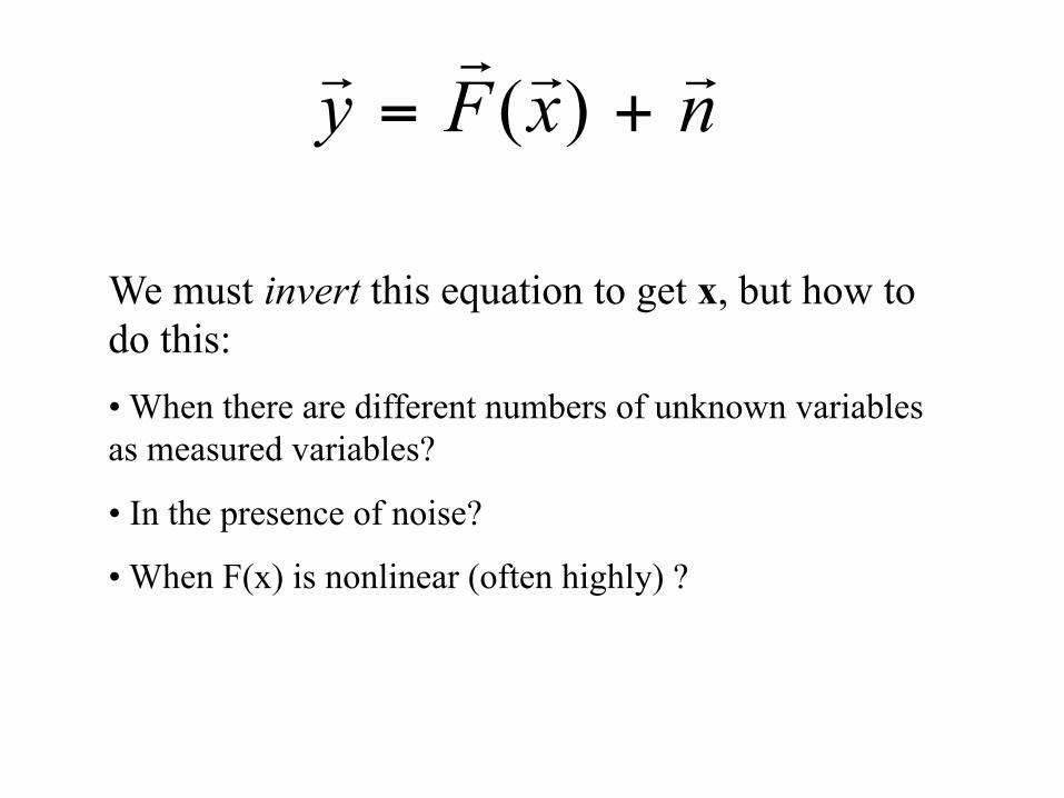
nxFy !!!!+= )(

We must invert this equation to get x, but how to do this: •  When there are different numbers of unknown variables as measured variables?

•  In the presence of noise?

•  When F(x) is nonlinear (often highly) ?

Retrieval Solution Techniques

•  Direct Solution (requires invertible forward model and same number of measured quantities as unknowns)

•  Multiple Linear Regression

•  Semi-Empirical Fitting

•  Neural Networks

•  Optimal Estimation Theory

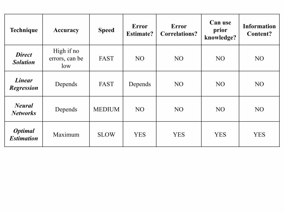
Technique Accuracy Speed Error Estimate?

Error Correlations?

Can use prior

knowledge?

Information Content?

Direct Solution

High if no errors, can be

low FAST NO NO NO NO

Linear Regression Depends FAST Depends NO NO NO

Neural Networks Depends MEDIUM NO NO NO NO

Optimal Estimation Maximum SLOW YES YES YES YES

Cloud Optical Thickness and Effective Radius

A Simple Example:

•  Cloud Optical Thickness and Effective Radius are often derived with a look-up table approach, although errors are not given.

•  The inputs are typically 0.86 micron and 2.06 micron reflectances from the cloud top.

water cloud forward calculations from Nakajima and King 1990

•  x = { reff, τ }

•  y = { R0.86 , R2.13 , ... }

•  Forward model must map x to y. Mie Theory, simple cloud droplet size distribution, radiative transfer model.

Simple Solution: The Look-up Table Approach

1.  Assume we know .

2.  Regardless of noise, find such that

3.  But is a vector! Therefore, we minimize the χ2 :

4.  Can make a look-up table to speed up the search.

x̂)(xF !

!

)(xFy !!!!−=ε is minimized.

ε!

∑−

=i i

ii xFy2

22 ))((

σχ

!

Example:

xtrue : { reff = 15 µm, τ = 30 }

Errors determined by how much change in each parameter (reff , τ ) causes the χ2 to change by one unit.

BUT

•  What if the Look-Up Table is too big?

•  What if the errors in y are correlated?

•  How do we account for errors in the forward model?

•  Shouldn’t the output errors be correlated as well?

•  How do we incorporate prior knowledge about x ?

Correlated Errors

•  Variables: y1, y2 , y3 ...

•  1-sigma errors: σ1 , σ2 , σ3 ...

•  The correlation between y1 and y2 is c12 (between –1 and 1), etc.

•  Then, the Noise Covariance Matrix is given by:

⎥⎥⎥⎥⎥

⎦

⎤

⎢⎢⎢⎢⎢

⎣

⎡

=

!"""###

2332233113

3223222112

3113211221

σσσσσ

σσσσσ

σσσσσ

cccccc

Sy

Example: Temperature Profile Climatology for December over Hilo, Hawaii

P = (1000, 850, 700, 500, 400, 300) mbar

<T> = (22.2, 12.6, 7.6, -7.7, -19.5, -34.1) Celsius

1.00 0.47 0.29 0.21 0.21 0.16 0.47 1.00 0.09 0.14 0.15 0.11 0.29 0.09 1.00 0.53 0.39 0.24 0.21 0.14 0.53 1.00 0.68 0.40 0.21 0.15 0.39 0.68 1.00 0.64 0.16 0.11 0.24 0.40 0.64 1.00

Correlation Matrix:

2.71 1.42 1.12 0.79 0.82 0.71 1.42 3.42 0.37 0.58 0.68 0.52 1.12 0.37 5.31 2.75 2.18 1.45 0.79 0.58 2.75 5.07 3.67 2.41 0.82 0.68 2.18 3.67 5.81 4.10 0.71 0.52 1.45 2.41 4.10 7.09

Covariance Matrix:

•  But what do we minimize ? Before, we found xhat such that this was a minimum:

∑

−=

i i

ii xFy2

22 ))((

σχ

!

•  Now, we must minimize the generalized χ2 :

( ) ( ))()( 12 xFySxFy yT !!!!!!

−−= −χ

•  This is just a number (a scalar), and reduces to the first equation when all the correlations are zero.

What to Minimize

Prior Knowledge

•  Prior knowledge about x can be known from many different sources, like other measurements or a weather or climate model prediction or climatology.

•  In order to specify prior knowledge of x, called xa , we must also specify how well we know xa; we must specify the errors on xa .

•  The errors on xa are generally characterized by a Probability Distribution Function (PDF) with as many dimensions as x.

•  For simplicity, people often assume prior errors to be Gaussian; then we simply specify Sa, the error covariance matrix associated with xa .

The χ2 with prior knowledge:

( ) ( )( ) ( )xxSxx

xFySxFy

aaT

a

yT

!!!!

!!!!!!

−−

+−−=−

−

1

12 )()(χ

Yes, that is a scary looking equation. But it is not so bad...

Minimization Techniques Minimizing the χ2 is hard. In general, you can use a look-

up table (this still works, if you have tabulated values of F(x) ), but if the lookup table approach is not feasible (i.e., it’s too big), then you have to do iteration:

1.  Pick a guess for x, called x0 .

2.  Calculate (or look up) F(x0) .

3.  Calculate (or look up) the Jacobian Matrix about x0:

j

iij x

xFxK∂

∂=

)()(!

!

K is the matrix of sensitivities, or derivatives, of each output (y) variable with respect to each input (x) variable. It is not necessarily square.

4.  Finally, iterate to get the next guess:

( ) ( )( )iaaiyTiiii xxSxFySKSxx !!!!!!!

−+−+= −−+

111 )(

( ) 111 −−− += aiyTii SKSKS

where:

xxFxKK i

ii !!!

!∂

∂==

)()(

Iteration in practice:

•  Not guaranteed to converge.

•  Can be slow, depends on non-linearity of F(x).

•  There are many tricks to make the iteration faster and more accurate.

•  Often, only a few function iterations are necessary.

Error Correlations?

xtrue reff = 15 µm, τ = 30 reff = 12 µm, τ = 8

{R0.86 , R2.13}true 0.796 , 0.388 0.516, 0.391

{R0.86 , R2.13}measured 0.808 , 0.401 0.529, 0.387

xderived reff = 14.3 µm, τ = 32.3 reff = 11.8 µm, τ = 7.6

Formal 95% Errors ± 1.5 µm, ± 3.7 ± 2.2 µm, ± 0.7

{reff, τ} Correlation 5% 55%

So, again, what is optimal estimation? Optimal Estimation is a way to infer information about a system, based on observations. It is necessary to be able to simulate the observations, given complete knowledge of the system state.

Optimal Estimation can:

•  Combine different observations of different types.

•  Utilize prior knowledge of the system state (climatology, model forecast, etc).

•  Errors are automatically provided, as are error correlations.

•  Estimate the information content of additional measurements.

Applications of Optimal Estimation

•  Retrieval Theory (standard, or using climatology, or using model forecast. Combine radar & satellite. Combine multiple satellites. Etc.)

•  Data Assimilation – optimally combine model forecast with measurements. Not just for weather! Example: carbon source sink models, hydrology models.

•  Channel Selection: can determine information content of additional channels when retrieving certain variables. Example: SIRICE mission is using this technique to select their IR channels to retrieve cirrus IWP.