Embed Size (px)
Citation preview

Lectures 3: Bayesian estimation ofspatial regression models
James P. LeSage
University of Toledo
Department of Economics
Toledo, OH 43606
March 2004

Introduction
• Application of Bayesian estimation methods to SAR,
SDM and SEM spatial regression models where the
number of observations is very large should result
in estimates nearly identical to those from maximum
likelihood methods.
• A standard result in econometrics because prior
information is dominated by a large amount of sample
information.
• Three points,
1) Bayesian methods can solve the problem of
inference in maximum likelihood computed using
numerial hessians, which are not always very good.
2) Bayesian methods can be used to relax the
assumption of constant variance normal disturbances
made by maximum likelihood methods, resulting in
extended models.
3) Bayesian methods can be used to formally
solve model comparison problems. We can
compare models based on: different weight matrices,
different explanatory (X) variables, or different model
specifications, e.g., SAR, SDM, SEM.
• We can develop Bayesian variants of the SAR, SDM and
SEM models that generalize on maximum likelihood by
allowing for non-constant variance over space.
1

ALL Bayesian econometric theory in 2overheads
In econometrics we care about 1) inference about
parameters, 2) model comparisons, and 3) prediction.
• p(A, B) = p(A|B)p(B) basic probability rules for
A, B r.v.
• p(A, B) = P (B|A)p(A) basic probability rules
• setting these two equal and rearranging yields Bayes’Rule
p(B|A) =p(A|B)p(B)
p(A)(1)
• Letting y = A represent model data and θ = B denote
model parameters:
P (θ|y) =p(y|θ)p(θ)
p(y)(2)
• With reference to 1) inference, All Bayesian
learning/inference about θ|y is based on the posterior
P (θ|y). Since we don’t care to learn about p(y),
because it doesn’t involve the parameters θ, our object
of interest we can simplify to:
p(θ|y) = p(y|θ)p(θ) (3)
2

Overhead #2
• With reference to 2) model comparison, each of m
models is denoted by a likelihood function and prior,
p(θi|y, Mi) =
p(y|θi, Mi)p(θi|Mi)
p(y|Mi)(4)
• Use Bayes’ rule again to explode terms like p(y|Mi) to
arrive at the posterior model probabilities, the basis for
inference about different models, given the sample data.
p(Mi|y) =p(y|Mi)p(Mi)
p(y)(5)
• p(y|Mi) is called the marginal likelihood and we can
solve for this key quantity needed for model comparison
finding:
p(y|Mi) =
Zp(y|θi
, Mi)p(θi|Mi)dθ
i(6)
• to avoid dealing with p(y), we can find:
POij =p(Mi|y)
p(Mj|y)=
p(y|Mi)p(Mi)
p(y|Mj)p(Mj)(7)
• With reference to 3) prediction of y? based on y, using
rules of probability:
p(y?|y) =
Zp(y
?, θ|y)dθ =
Zp(y
?|y, θ)p(θ|y)dθ
(8)
3

Markov Chain Monte Carlo estimation
Bayesian ordinary least-squares regression (non-spatial
example)
y = Xβ + ε (9)
ε ∼ N(0, σ2In)
The parameters to be estimated in (9) are (β, σ), for
which we assign a prior density of the form π(β, σ) =
π1(β)π2(σ), with a normal prior for β and diffuse prior for
σ.
Rβ ∼ N(r, T ) (10)
π1(β) ∝ exp{−(1/2)(Rβ − r)′T−1
(Rβ − r)}
π2(σ) ∝ (1/σ)
(Like Theil and Goldberger (1961) regression.)
For our purposes it is convenient to express (10) in an
alternative (equivalent) form based on a factorization of T−1
into Q′Q = T−1, and q = Qr leading to (11).
4

Qβ ∼ N(q, Im) (11)
π1(β) ∝ exp{−(1/2)(Qβ − q)′(Qβ − q)}
Following the usual Bayesian methodology, we combine
the likelihood function for our simple model:
L(β, σ) ∝ (1/σn)exp[(y−Xβ)
′(y−Xβ)/2σ
2] (12)
with the priors π1(β) and π2(σ) to produce the posterior
density for (β, σ) shown in (13).
p(β, σ) ∝ (1/σn+1
)exp[β − β̂(σ)]′[V (σ)]
−1[β − β̂(σ)]
β̂(σ) = (X′X + σ
2Q
′Q)
−1(X
′y + σ
2Q
′q)
V (σ) = σ2(X
′X + σ
2Q
′Q)
−1(13)
In (13), we have used the notation β̂(σ) to convey
that the mean of the posterior, β̂, is conditional on the
parameter σ, as is the variance, denoted by V (σ). This
single parameter prevents analytical solution of the Bayesian
regression problem.
5

In order to overcome this problem, Theil and Goldberger
(1961) observed that conditional on σ, the posterior density
for β is multivariate normal. They proposed that σ2 be
replaced by an estimated value, σ̂2, based on least-squares
estimates β̂.
β̂TG = (X′X + σ̂
2Q
′Q)
−1(X
′y + σ̂
2Q
′q)
var(β̂TG) = σ̂2(X
′X + σ̂
2Q
′Q)
−1(14)
The advantage of this solution is that the estimation
problem can be solved using existing least-squares regression
software. Their solution produces a point estimate which we
label β̂TG and an associated variance-covariance estimate,
both of which are shown in (14).
6

An MCMC Sampling solution
The Gibbs sampler provides a way to sample from a
multivariate probability density based only on the densities
of subsets of vectors conditional on all others.
A two-step Gibbs sampler for the posterior distribution
(13) of our Bayesian regression model based on the
distribution of β conditional on σ and the distribution of σ
conditional on β. For our regression problem, the posterior
density for β conditional on σ, p(β|σ), is multivariate
normal with mean equal to and variance as indicated in (15).
p(β|σ) ∼ N [β̂(σ), V (σ)] (15)
β̂(σ) = (X′X + σ
2Q
′Q)
−1(X
′y + σ
2Q
′q)
V (σ) = σ2(X
′X + σ
2Q
′Q)
−1
The posterior density for σ conditional on β, p(σ|β) is:
p(σ|β) ∝ (e′e)/χ
2(n)(16)
(y − Xβ)′(y − Xβ)/σ
2|β ∼ χ2(n)
7
The Gibbs sampler suggested by these two conditional
posterior distributions involves the following computations.
• Begin with arbitrary values for the parameters β0 and
σ0, which we designate with the superscript 0.
• Compute the mean and variance of β ∼N [β̂(σ), V (σ)] using (15) conditional on the initial
value σ0.
• Use the computed mean and variance of β to draw a
multivariate normal random vector, which we label β1.
• Use the value β1 along with a random χ2(n) draw to
determine σ1 using (16).
The above four steps are known as a ‘single pass’ through
our (two-step) Gibbs sampler, where we have replaced the
initial arbitrary values of β0 and σ0 with new values labeled
β1 and σ1. We now return to step using the new values β1
and σ1 in place of the initial values β0 and σ0, and make
another ‘pass’ through the sampler. This produces a new set
of values, β2 and σ2.
8

An Example% ----- A simple Gibbs samplern=100; k=3; % set nobs and nvarsx = randn(n,k); % generate data setb = ones(k,1);y = x*b + randn(n,1);r = [1.0 1.0 1.0]’; % prior meansR = eye(k); T = eye(k); % prior varianceQ = chol(inv(T)); Qpr = Q*r; % convenience transformb0 = (x’*x)\(x’*y); % use ols as initial valuessige = (y-x*b0)’*(y-x*b0)/(n-k);ndraw = 6000; nomit = 1000; % set the number of drawsbsave = zeros(ndraw,k); % allocate storage for resultsssave = zeros(ndraw,1);xpx = x’*x; xpy = x’*y; % compute these before samplingtic;for i=1:ndraw; % Start the samplingxpxi = inv(xpx + sige*Q);xpyi = (xpy + sige*Qpr);% update bb = xpxi*xpyi;b = norm_rnd(sige*xpxi) + b;bsave(i,:) = b’;% update sigee = y - x*b;chi = chis_rnd(1,n);sige = e’*e/chi;ssave(i,1) = sige;end; % End the samplingtoc;bhat = mean(bsave(nomit+1:ndraw,:)); % calculate meansbstd = std(bsave(nomit+1:ndraw,:)); % and std deviationsshat = mean(ssave(nomit+1:ndraw,1));
9

Results
Gibbs estimates (1.22 seconds for 6,000 draws)Variable Coefficient t-statistic t-probabilityvariable 1 1.101726 9.507527 0.000000variable 2 1.034981 9.637922 0.000000variable 3 0.994645 9.326300 0.000000
Theil-Goldberger Regression EstimatesR-squared = 0.7376Rbar-squared = 0.7321sigma^2 = 1.0071Durbin-Watson = 1.8900Nobs, Nvars = 100, 3***************************************************************Variable Prior Mean Std Deviationvariable 1 1.000000 1.000000variable 2 1.000000 1.000000variable 3 1.000000 1.000000***************************************************************
Posterior EstimatesVariable Coefficient t-statistic t-probabilityvariable 1 1.099942 9.512551 0.000000variable 2 1.035667 9.804278 0.000000variable 3 0.995215 9.490806 0.000000
10

Bayesian spatial models
Similar to the least-squares model we already did.
Parameters are: β, σ, ρ. We need the conditional
distributions for each of these, and then we can develop
a sampler.
A normal-gamma conjugate prior for β and σ, and a
uniform prior for ρ. The prior distributions are indicated
using π.
y = ρWy + Xβ + ε
ε ∼ N(0, σ2In)
π(β) ∼ N(c, T )
π(1/σ2) ∼ Γ(d, ν)
π(ρ) ∼ U [0, 1]
(17)
11

In the case of large samples involving 3,000 observations,
the normal-gamma priors for β, σ should exert relatively little
influence. Setting c to zero and T to a very large number
results in a diffuse prior for β. Diffuse settings for σ involve
setting d = 0, ν = 0. For completeness, we develop the
results for the case of a normal-gamma prior on β, σ.
In contrast to the case of the priors on β, σ, assigning
an informative prior to the parameter ρ associated with
spatial dependence should exert an impact on the estimation
outcomes even in large samples. This is due the important
role played by spatial dependence in these models. In typical
applications where the magnitude and significance of ρ is
a subject of interest, a diffuse prior would be used. It is
however possible to rely on an informative prior for this
parameter.
The parameters β, σ and ρ in the SAR model can
be estimated by drawing sequentially from the conditional
distributions of these parameters.
12

Conditional distributions
To implement this estimation method, we need to
determine the conditional distributions for each parameter in
our Bayesian SAR model.
• The conditional distribution for β follows from the
maximum likelihood model:
p(β|ρ, σ) ∼ N(b̄, σ2B) (18)
b̄ = A(X′Sy + σ
2T−1
c)
B = σ2A
A = (X′X + σ
2T−1
)−1
S = (In − ρW )
We see that the conditional for β is a multivariate normal
distribution from which it is easy to sample a vector β.
• The conditional distribution for σ given the other
parameters, takes the form (see Gelman, Carlin, Stern
and Rubin, 1995):
p(σ2|β, ρ) ∝ (σ
2)−(n
2+d+1)exp
�−e
′e +
2ν
2σ2
�
e = (In − ρW )y − Xβ
13

which is proportional to an inverse gamma distribution
with parameters (n/2) + d and e′e + 2ν. Again, this
would be an easy distribution from which to sample a
scalar value for σ.
• Finally, the conditional posterior distribution of ρ takes
the form:
p(ρ|β, σ) ∝ |S(ρ)|(s2(ρ))
−(n−k)/2π(ρ) (19)
s2(ρ) =
(Sy − Xb(ρ))′(Sy − Xb(ρ))
(n − k)
S = (In − ρW )
A problem arises here in that this distribution is not one
for which established algorithms exist to produce random
draws.
There are however two ways to sample from this
conditional distribution.
1) Use Metropolis-Hastings algorithms.
2) A griddy Gibbs sampler, with univariate
numerical integration to find the conditional posterior
distribution and then carry out a draw using
“inversion”.
14

The MCMC sampler
By way of summary, an MCMC estimation scheme
involves starting with arbitrary initial values for the
parameters which we denote β0, σ0, V 0, ρ0. We then
sample sequentially from the following set of conditional
distributions for the parameters in our model.
• p(β|σ0, ρ0, ), which is a multivariate normal distribution
with mean and variance defined in (18). This updated
value for the parameter vector β we label β1.
• p(σ|β1, ρ0), which is chi-squared distributed with n+2d
degrees of freedom. Note that we rely on the updated
value of the parameter vector β = β1 when evaluating
this conditional density. We label the updated parameter
σ = σ1 and note that we will continue to employ the
updated values of previously sampled parameters when
evaluating the next conditional densities in the sequence.
• p(ρ|β1, σ1, which we could sample using a metropolis
step or univariate numerical integration and inversion.
15
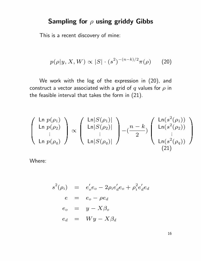
Sampling for ρ using griddy Gibbs
This is a recent discovery of mine:
p(ρ|y, X, W ) ∝ |S| · (s2)−(n−k)/2
π(ρ) (20)
We work with the log of the expression in (20), and
construct a vector associated with a grid of q values for ρ in
the feasible interval that takes the form in (21).
0BB@
Ln p(ρ1)
Ln p(ρ2)...
Ln p(ρq)
1CCA ∝
0BB@
Ln|S(ρ1)|Ln|S(ρ2)|
...
Ln|S(ρq)|
1CCA−(
n − k
2)
0BB@
Ln(s2(ρ1))
Ln(s2(ρ2))...
Ln(s2(ρq))
1CCA
(21)
Where:
s2(ρi) = e
′oeo − 2ρie
′deo + ρ
2i e
′ded
e = eo − ρed
eo = y − Xβo
ed = Wy − Xβd
16

βo = (X′X)
−1X
′y
βd = (X′X)
−1X
′Wy (22)
This vector allows univariate numerical integration using
a simple method such as Simpson’s rule. For this model,
you can compute the log-determinant once before you begin
sampling.
17

Computational issues using griddy Gibbs
There are four separate terms involved in the univariate
integration problem over the range of support for the
parameter ρ. These are shown in (23) as T1, T2, T3 and T4.
In addition, there are constants of proportionality that arise
during the analytical integration of β and σ that include a
Gamma function that involves n − k, where n denotes the
number of observations and k the number of explanatory
variables. For cases involving model comparisons where
the number of explanatory variables k varies, we need also
include this expression during solution of our integration
problem, which we will refer to as T0.
T1(ρ) = |In − ρW | (23)
T2 = |X ′X|−1/2
T3(ρ) = s2(ρ)
−(n−k)/2
s2(ρ) = {[(In − ρW )y − Xβ]
′[(In − ρW )y − Xβ]}
T4(ρ) =1
Be(α, α)
(1 + ρ)α−1(1 − ρ)α−1
22α−1
18

Griddy Gibbs sampling for rho
0 0.1 0.2 0.3 0.4 0.5 0.6 0.7 0.8 0.9 10
0.2
0.4
0.6
0.8
1
1.2
1.4
uniform 0,1 values
rho
draw
cumulative marginaldistribution for rho
Figure 1: Griddy Gibbs sampling for ρ
19

Applied examples
load elect.dat; % load data on votesy = log(elect(:,7)./elect(:,8));x1 = log(elect(:,9)./elect(:,8));x2 = log(elect(:,10)./elect(:,8));x3 = log(elect(:,11)./elect(:,8));latt = elect(:,5);long = elect(:,6);n = length(y); x = [ones(n,1) x1 x2 x3];n = 3107;[junk W junk] = xy2cont(latt,long);vnames = strvcat(’voters’,’const’,’educ’,’homeowners’,’income’);
result = sar(y,x,W); % maximum likelihood estimatesprt(result,vnames);
ndraw = 2500; nomit = 500;prior.novi = 1; % homoscedastic modelresult2 = sar_g(y,x,W,ndraw,nomit,prior); % MCMC estimationresult2.tflag = ’tstat’;prt(result2,vnames);plt(result2);
result = sdm(y,x,W); % maximum likelihood estimatesprt(result,vnames);
ndraw = 2500;nomit = 500;prior.novi = 1; % homoscedastic modelresult2 = sdm_g(y,x,W,ndraw,nomit,prior); % MCMC estimationresult2.tflag = ’tstat’;prt(result2,vnames);
20

Results
sar: hessian not positive definite augmenting small eigenvalues
Spatial autoregressive Model EstimatesDependent Variable = votersR-squared = 0.4426Rbar-squared = 0.4420sigma^2 = 0.0138Nobs, Nvars = 3107, 4log-likelihood = 3209.629# of iterations = 12min and max rho = 0.0000, 1.0000total time in secs = 1.2710time for lndet = 0.8010time for t-stats = 0.2000Pace and Barry, 1999 MC lndet approximation usedorder for MC appr = 50iter for MC appr = 30***************************************************************Variable Coefficient Asymptot t-stat z-probabilityconst 0.626492 20.910168 0.000000educ 0.220617 26.439243 0.000000homeowners 0.481831 48.551766 0.000000income -0.099245 -20.069609 0.000000rho 0.586990 41.899648 0.000000
21
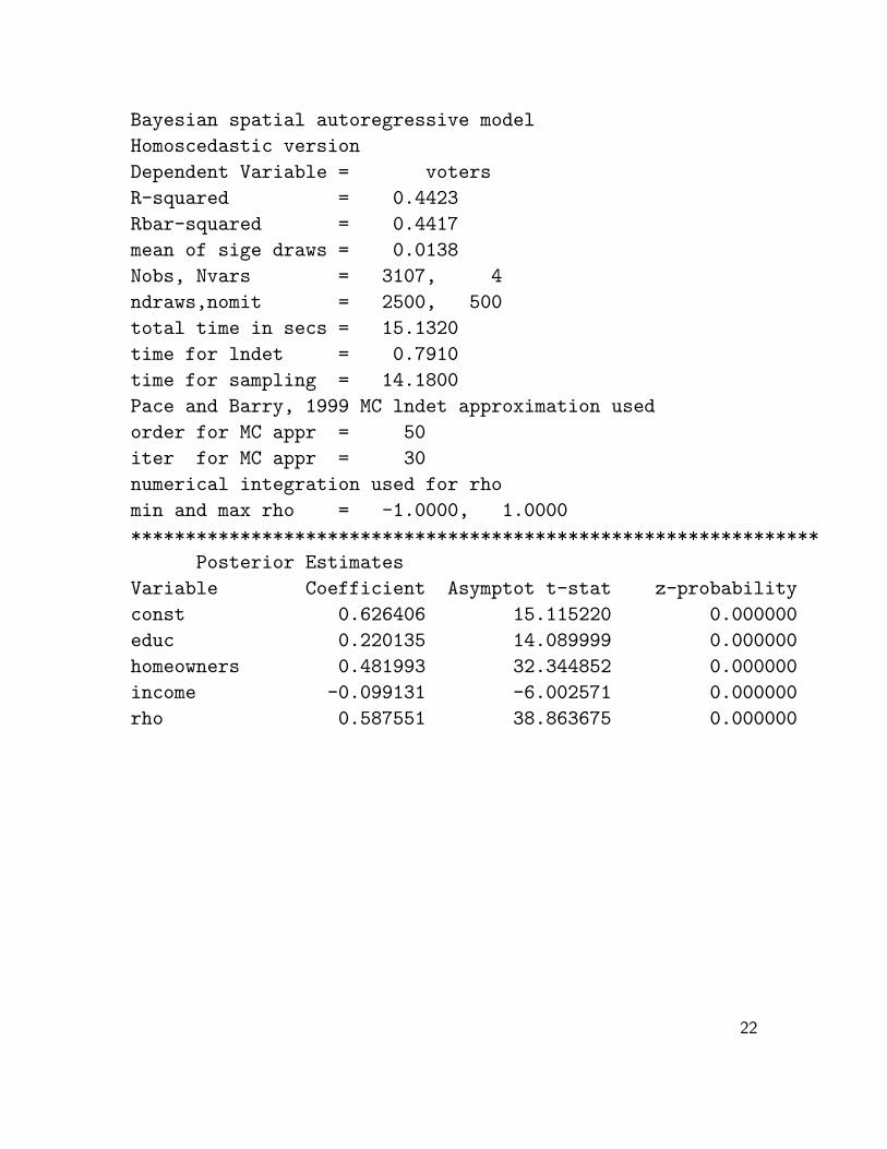
Bayesian spatial autoregressive modelHomoscedastic versionDependent Variable = votersR-squared = 0.4423Rbar-squared = 0.4417mean of sige draws = 0.0138Nobs, Nvars = 3107, 4ndraws,nomit = 2500, 500total time in secs = 15.1320time for lndet = 0.7910time for sampling = 14.1800Pace and Barry, 1999 MC lndet approximation usedorder for MC appr = 50iter for MC appr = 30numerical integration used for rhomin and max rho = -1.0000, 1.0000***************************************************************
Posterior EstimatesVariable Coefficient Asymptot t-stat z-probabilityconst 0.626406 15.115220 0.000000educ 0.220135 14.089999 0.000000homeowners 0.481993 32.344852 0.000000income -0.099131 -6.002571 0.000000rho 0.587551 38.863675 0.000000
22

sar: hessian not positive definite augmenting small eigenvalues
Spatial Durbin modelDependent Variable = votersR-squared = 0.5072Rbar-squared = 0.5063sigma^2 = 0.0126log-likelihood = 3316.1081Nobs, Nvars = 3107, 4# iterations = 17min and max rho = 0.0000, 1.0000total time in secs = 0.9920time for lndet = 0.7310time for t-stats = 0.1600Pace and Barry, 1999 MC lndet approximation usedorder for MC appr = 50iter for MC appr = 30***************************************************************Variable Coefficient Asymptot t-stat z-probabilityconst 0.466628 248.431325 0.000000educ 0.136006 5.507480 0.000000homeowners 0.581067 38.360260 0.000000income -0.069938 -3.036205 0.002396W-educ 0.107467 3.664551 0.000248W-homeowners -0.410606 -19.836192 0.000000W-income -0.077025 -2.695428 0.007030rho 0.653982 33.605980 0.000000
23

Bayesian Spatial Durbin modelHomoscedastic versionDependent Variable = votersR-squared = 0.5072mean of sige draws = 0.0126Nobs, Nvars = 3107, 7ndraws,nomit = 2500, 500total time in secs = 16.1930time for lndet = 0.7410time for sampling = 15.2620Pace and Barry, 1999 MC lndet approximation usedorder for MC appr = 50iter for MC appr = 30numerical integration used for rhomin and max rho= -1.0000, 1.0000***************************************************************Variable Coefficient Asymptot t-stat z-probabilityconst 0.461836 9.089562 0.000000educ 0.135410 5.314491 0.000000homeowners 0.580899 37.353203 0.000000income -0.069273 -3.005387 0.002652W-educ 0.106829 3.521691 0.000429W-homeowners -0.411537 -14.616216 0.000000W-income -0.076070 -2.476424 0.013271rho 0.655221 40.227536 0.000000
24

Using plt(results)
0 1000 2000 3000 4000�4
�3
�2
�1
0
1SAR heteroscedastic Gibbs Actual vs. Predicted
ActualPredicted
0 1000 2000 3000 40001.5
1
0.5
0
0.5
1
1.5Residuals
0 1000 2000 3000 40000
0.5
1
1.5
2Mean of Vi draws
0.5 0.55 0.6 0.65�5
0
5
10
15
20
25
30
Posterior Density for rho
Figure 2: plotting the results structure
25

Bayesian heteroscedastic/robust spatialmodels
We introduce a more general version of the SAR, SDM and SEMmodels that allows for non-constant variance across space as well asoutliers. When dealing with spatial datasets one can encounter whathave become known as “enclave effects”, where a particular region doesnot follow the same relationship as the majority of spatial observations.For example, all counties in a single state might represent aberrantobservations that differ from those in all other counties. This will lead tofat-tailed errors that are not normal, but more likely to follow a Student-tdistribution.
• Introduce a set of variance scalars (v1, v2, . . . , vn), as unknownparameters that need to be estimated.
• This allows us to assume ε ∼ N(0, σ2V ), where V =diag(v1, v2, . . . , vn).
• The prior distribution for the vi terms takes the form of anindependent χ2(r)/r distribution. Recall that the χ2 distributionis a single parameter distribution, where we have represented thisparameter as r. This allows us to estimate the additional nparameters vi in the model by adding the single parameter r to ourestimation procedure.
26

The heteroscedastic prior
0 0.5 1 1.5 2 2.5 30
0.2
0.4
0.6
0.8
1
1.2
1.4
prio
r pro
babi
lity
dens
ity
Vi values
r=2r=5r=20
Figure 3: Prior Vi distributions for various values of r
• The prior mean of the vi equals unity and the prior variance of thevi is 2/r.
• This implies that as r becomes very large, the terms vi will allapproach unity, resulting in V = In, the traditional assumption ofconstant variance across space.
• On the other hand, small values of r lead to a skewed distributionthat permits large values of vi that deviate greatly from the priormean of unity.
• The role of these large vi values is to accommodate outliers orobservations containing large variances by downweighting theseobservations.
27

• Note that ε ∼ N(0, σ2V ), with V diagonal implies a generalizedleast-squares (GLS) correction to the vector y and explanatoryvariables matrix X. The GLS correction involves dividing throughby
√vi, which leads to large vi values functioning to downweight
these observations. Even in large samples, this prior will exert animpact on the estimation outcome.
Bayesian heteroscedastic SAR model
A normal-gamma conjugate prior for β and σ, and a uniform priorfor ρ in addition to the chi-squared prior for the terms in V . The priordistributions are indicated using π.
y = ρWy + Xβ + ε
ε ∼ N(0, σ2V ) V = diag(v1, . . . , vn)
π(β) ∼ N(c, T )
π(r/vi) ∼ IIDχ2(r)
π(1/σ2) ∼ Γ(d, ν)
π(ρ) ∼ U [0, 1]
(24)
28

Estimation of Bayesian spatial models
An unfortunate complication that arises with this extension is thatthe addition of the chi-squared prior creates a complicated posteriordistribution. Assume for the moment, diffuse priors for β, σ. A keyinsight is that if we knew V , this problem would look like a GLS versionof the SAR model.
That is, conditional on V , we would arrive at similar expressions asin maximum likelihood, where the y and X are transformed by dividingthrough by:
pdiag(V ). We rely on a Markov Chain Monte Carlo
(MCMC) estimation method that exploits this fact.
The parameters β, V and σ in the heteroscedastic SAR model canbe estimated by drawing sequentially from the conditional distributionsof these parameters.
29

Conditional distributions
To implement this estimation method, we need to determinethe conditional distributions for each parameter in our Bayesianheteroscedastic SAR model.
• The conditional distribution for β follows from the insight that givenV , we can rely on standard Bayesian GLS regression results to showthat:
p(β|ρ, σ, V ) ∼ N(b̄, σ2B) (25)
β̄ = A(X′V−1
Sy + σ2T−1
c)
B = σ2A
A = (X′V−1
X + σ2T−1
)−1
We see that the conditional for β is a multivariate normal distributionfrom which it is easy to sample a vector β.
• The conditional distribution for σ given the other parameters, takesthe form (see Gelman, Carlin, Stern and Rubin, 1995):
p(σ2|β, ρ, V ) ∝ (σ
2)−(n
2+d+1)exp
�−e
′V−1
e +2ν
2σ2
�
e = (In − ρW )y − Xβ
which is proportional to an inverse gamma distribution withparameters (n/2) + d and e′V −1e + 2ν. Again, this wouldbe an easy distribution from which to sample a scalar value for σ.
• Geweke (1993) shows that the conditional distribution of V given theother parameters is proportional to a chi-square density with r + 1
30

degrees of freedom. Specifically, we can express the conditionalposterior of each vi as:
p(e2i + r
vi|β, ρ, σ
2, v−i) ∼ χ
2(r + 1) (26)
where v−i = (v1, . . . , vi−1, vi+1, . . . , vn) for each i, and e isas defined above. Again, this represents a known distribution fromwhich it is easy to construct a scalar draw.
• Finally, the conditional posterior distribution of ρ takes the form:
p(ρ|β, σ, V ) ∝ |S(ρ)|(s2(ρ))
−(n−k)/2π(ρ) (27)
s2(ρ) =
(Sy − Xb(ρ))′V −1(Sy − Xb(ρ))
(n − k)
Again, we can use either Metropolis-Hastings or univariate numericalintegration to draw ρ values.
31

Example code
while (iter <= ndraw); % ============> start sampling;xs = matmul(x,sqrt(V)); % ============> update betays = sqrt(V).*y; Wys = sqrt(V).*Wy;AI = inv(xs’*xs + sige*TI);yss = ys - rho*Wys;b = xs’*yss + sige*TIc;b0 = AI*b;bhat = norm_rnd(sige*AI) + b0;xb = xs*bhat;nu1 = n + 2*nu; % ============> update sigee = (yss - xb); d1 = 2*d0 + e’*e;chi = chis_rnd(1,nu1);sige = d1/chi;ev = y - rho*Wy - xb; % ============> update vichiv = chis_rnd(n,rval+1);vi = ((ev.*ev/sige) + in*rval)./chiv;V = in./vi;b0 = AI*xs’*ys; % ============> update rhobd = AI*xs’*Wys;e0 = ys - xs*b0; ed = Wys - xs*bd;epe0 = e0’*e0;eped = ed’*ed;epe0d = ed’*e0;rho = draw_rho(detval,epe0,eped,epe0d,n,k,rho);bsave(iter,1:k) = bhat’;% ============> save drawsssave(iter,1) = sige;psave(iter,1) = rho;vmean = vmean + vi;
iter = iter + 1;end; % ============> end sampling
32

Applied Example
To illustrate the heteroscedastic Bayesian SAR model,
generate data with outliers.
y = (In − ρW )−1
Xβ + (In − ρW )−1
ε (28)
load anselin.dat; % 49 observations from Columbus, OHlatt = anselin(:,4); long = anselin(:,5);% create W-matrix using Anselin’s neigbhorhood crime data set[junk W junk] = xy2cont(latt,long);[n junk] = size(W); k = 3; IN = eye(n);sige = 0.1; rho = 0.7; % true values for sige and rhox = randn(n,k); % generate random normal X-matrixbeta = ones(k,1); % true parameter valuesndraw = 2500; % # of draws to carry outnomit = 500; % # of draws to exclude for burn-in% generate y based on the SAR modelout = ones(n,1);out(30,1) = 10; out(35,1) = 10; out(40,1) = 10;y = inv(IN-rho*W)*x*beta + inv(IN-rho*W)*randn(n,1).*out;% estimate maximum likelihood modelresult = sar(y,x,W);prt(result);prior.rval = 4; % heteroscedastic priorresult2 = sar_g(y,x,W,ndraw,nomit,prior);prt(result2);
33

Results
Spatial autoregressive Model EstimatesR-squared = 0.4525Rbar-squared = 0.4287sigma^2 = 8.5044Nobs, Nvars = 49, 3log-likelihood = 108.95304# of iterations = 16min and max rho = -1.0000, 1.0000total time in secs = 0.1000time for lndet = 0.0600time for t-stats = 0.0100Pace and Barry, 1999 MC lndet approximation usedorder for MC appr = 50iter for MC appr = 30***************************************************************Variable Coefficient Asymptot t-stat z-probabilityvariable 1 0.557826 1.087610 0.276767variable 2 1.082276 2.589818 0.009603variable 3 -0.082036 -0.188551 0.850445rho 0.766955 4.667705 0.000003
34

Results
Bayesian spatial autoregressive modelHeteroscedastic modelR-squared = 0.4657sigma^2 = 1.0282r-value = 4Nobs, Nvars = 49, 3ndraws,nomit = 2500, 500total time in secs = 13.9300time for lndet = 0.0600time for sampling = 13.8500Pace and Barry, 1999 MC lndet approximation usedorder for MC appr = 50iter for MC appr = 30numerical integration used for rhomin and max rho = -1.0000, 1.0000***************************************************************
Posterior EstimatesVariable Coefficient Std Deviation p-levelvariable 1 0.761523 0.229360 0.000500variable 2 0.758247 0.170338 0.000000variable 3 0.727195 0.193013 0.000000rho 0.768175 0.056886 0.000000
35

0 5 10 15 20 25 30 35 40 45 50�5
0
5
10
15
20
25SAR model Actual vs. Predicted
ActualPredicted
0 5 10 15 20 25 30 35 40 45 50�5
0
5
10
15
20Residuals
Figure 4: Maximum likelihood act/pred and residuals
0 5 10 15 20 25 30 35 40 45 500
5
10
15
20
25
30
35
40Viestimates
Observations
Figure 5: Posterior means of the vi estimates
36