Embed Size (px)
Citation preview

CompSci 590.6 Understanding Data: Theory and Applica>ons
Lecture 2 Data Cube Basics
Instructor: Sudeepa Roy Email: [email protected]
1

Today’s Papers 1. Gray-‐Chaudhuri-‐Bosworth-‐Layman-‐Reichart-‐Venkatrao-‐Pellow-‐Pirahesh Data Cube: A Rela-onal Aggrega-on Operator Generalizing Group-‐By, Cross-‐Tab, and Sub-‐Totals ICDE 1996/Data Mining and Knowledge Discovery 1997
– Thinking process at that >me
2. Agarwal-‐Agrawal-‐Deshpande-‐Gupta-‐Naughton-‐Ramakrishnan-‐Sarawagi On the Computa-on of Mul-dimensional Aggregates VLDB 1996
– Technical
(more than 2630 and 750 cita>ons resp. on Google Scholar)
2

Naïve Approach • Data analysts are interested in exploring trends and
anomalies • Possibly by visualiza>on (Excel) -‐ 2D or 3D plots • “Dimensionality Reduc>on” by summarizing data and
compu>ng aggregates
• Find total unit sales for each 1. Model 2. Model, broken into years 3. Year, broken into colors 4. Year 5. Model, broken into colors 6. ….
3
Year Color
Mod
el
Sales (Model, Year, Color, Units)
Total Unit sales

Naïve Approach Run a number of queries SELECT sum(units) FROM Sales SELECT Color, sum(units) FROM Sales GROUP BY Color SELECT Year, sum(units) FROM Sales GROUP BY Year SELECT Model, Year, sum(units) FROM Sales GROUP BY Model, Year ….
• Data cube generalizes Histogram, Roll-‐Ups,
Cross-‐Tabs • More complex to do these with GROUP-‐BY
4
• How many sub-‐queries? • How many sub-‐queries for
8 ahributes?
Sales (Model, Year, Color, Units)
Year Color
Mod
el
Total Unit sales

Histograms A tabulated frequency of computed values
SELECT Year, COUNT(Units) as total FROM Sales
GROUP BY Year
ORDER BY Year
May require a nested SELECT to compute
Sales (Model, Year, Color, Units)
Year -‐>
total -‐>

Roll-‐Ups • Analysis reports start at a coarse level,
go to finer levels • Order of ahribute mahers • Not rela>onal data (empty cells no
keys)
Model Year Color Model, Year, Color Model, Year Model
Chevy 1994 Black 50
Chevy 1994 White 40
90
Chevy 1995 Black 115
Chevy 1995 White 85
200
290
GROUP BY
Sales (Model, Year, Color, Units)
Roll-‐ups
Drill-‐downs

Roll-‐Ups • Another representa>on (Chris Date’96) • Rela>onal, but
– long ahribute names – hard to express in SQL and repe>>on
Model Year Color Model, Year, Color Model, Year Model
Chevy 1994 Black 50 90 290
Chevy 1994 White 40 90 290
Chevy 1995 Black 85 200 290
Chevy 1995 Black 115 200 290
GROUP BY
Sales (Model, Year, Color, Units)

‘ALL’ Construct Easier to visualize roll-‐up if allow ALL to fill in the super-‐aggregates
SELECT Model, Year, Color, SUM(Units) FROM Sales WHERE Model = ‘Chevy’
GROUP BY Model, Year, Color
UNION SELECT Model, Year, ‘ALL’, SUM(Units)
FROM Sales
WHERE Model = ‘Chevy’ GROUP BY Model, Year
UNION …
UNION SELECT ‘ALL’, ‘ALL’, ‘ALL’, SUM(Units)
FROM Sales
WHERE Model = ‘Chevy’;
Model Year Color Units
Chevy 1994 Black 50
Chevy 1994 White 40
Chevy 1994 ‘ALL’ 90
Chevy 1995 Black 85
Chevy 1995 White 115
Chevy 1995 ‘ALL’ 200
Chevy ‘ALL’ ‘ALL’ 290
Sales (Model, Year, Color, Units)

Model Year Color Units
Chevy 1994 Black 50
Chevy 1994 White 40
Chevy 1994 ‘ALL’ 90
Chevy 1995 Black 85
Chevy 1995 White 115
Chevy 1995 ‘ALL’ 200
Chevy ‘ALL’ ‘ALL’ 290
Model Year Color Model, Year, Color Model, Year Model
Chevy 1994 Black 50
Chevy 1994 White 40
90
Chevy 1995 Black 115
Chevy 1995 White 85
200
290
Tradi>onal Roll-‐Up ‘ALL’ Roll-‐Up
• Roll-‐ups are asymmetric
Sales (Model, Year, Color, Units)

Cross Tabula>on If we made the roll-‐up symmetric, we would get a cross-‐tabula>on Generalizes to higher dimensions
SELECT Model, ‘ALL’, Color, SUM(Units)
FROM Sales
WHERE Model = ‘Chevy’
GROUP BY Model, Color
Chevy 1994 1995 Total (ALL)
Black 50 85 135
White 40 115 155
Total (ALL) 90 200 290
Is the problem solved with Cross-‐Tab and GROUP-‐BYs with ‘ALL’? • Requires a lot of GROUP BYs (64 for 6-‐dimension) • Too complex to op>mize (64 scans, 64 sort/hash, slow)
Sales (Model, Year, Color, Units)

Data Cube: Intui>on SELECT ‘ALL’, ‘ALL’, ‘ALL’, sum(units)
FROM Sales
UNION
SELECT ‘ALL’, ‘ALL’, Color, sum(units)
FROM Sales
GROUP BY Color
UNION SELECT ‘ALL’, Year, ‘ALL’, sum(units)
FROM Sales
GROUP BY Year
UNION SELECT Model, Year, ‘ALL’, sum(units)
FROM Sales
GROUP BY Model, Year
UNION ….
11
Sales (Model, Year, Color, Units)
Year Color
Mod
el
Total Unit sales

Data Cube
Ack: from slides by Laurel Orr and Jeremy Hyrkas, UW

Data Cube • Computes the aggregate on all possible combina>ons of
group by columns.
• If there are N ahributes, there are 2N-‐1 super-‐aggregates.
• If the cardinality of the N ahributes are C1,..., CN, then there are a total of (C1+1)...(CN+1) values in the cube.
• ROLL-‐UP is similar but just looks at N aggregates

Data Cube Syntax • SQL Server
SELECT Model, Year, Color, sum(units)
FROM Sales
GROUP BY Model, Year, Color
WITH CUBE
Sales (Model, Year, Color, Units)

Types of Aggregates
• Distribu>ve: input can be par>>oned into disjoint sets and aggregated separately o COUNT, SUM, MIN
• Algebraic: can be composed of distribu>ve aggregates o AVG
• Holis>c: aggregate must be computed over the en>re input set o MEDIAN

Types of Aggregates
Efficient computa>on of the CUBE operator depends on the type of aggregate
Distribu>ve and Algebraic aggregates mo>vate op>miza>ons

Agarwal et al paper
• Compute GROUP-‐BYs from previously computed GROUP-‐BYs
• Which direc>on?
• Next, some generic op>miza>ons

Op>miza>on 1: Smallest Parent • Compute GROUP-‐BY from
the smallest (size) previously computed GROUP-‐BY as a parent
– AB can be computed from ABC, ABD, or ABCD
– ABC or ABD beher than ABCD – Even ABC or ABD may have
different sizes
18
ABCD
ABC ABD ACD BCD
AC AD BC BD CD AB
A B C D
all

Op>miza>on 2: Cache Results • Cache result of one GROUP-‐
BY in memory to reduce disk I/O – Compute AB from ABC while
ABC is s>ll in memory
19
ABCD
ABC ABD ACD BCD
AC AD BC BD CD AB
A B C D
all

Op>miza>on 3: Amor>ze Disk Scans
• Amor>ze disk reads for mul>ple GROUP-‐Bys – Suppose the result for ABCD
is stored on disk – Compute all of ABC, ABD,
ACD, BCD simultaneously in one scan of ABCD
20
ABCD
ABC ABD ACD BCD
AC AD BC BD CD AB
A B C D
all

Op>miza>on 4, 5 (later) • 4. Share-‐sort
– for sort-‐based algorithms
• 5. Shared-‐par>>on – for hash-‐based algorithms
21
ABCD
ABC ABD ACD BCD
AC AD BC BD CD AB
A B C D
all

PipeSort Algorithm
22

PipeSort: Basic Idea • Share-‐sort op>miza>on:
– Data sorted in one order – Compute all GROUP-‐BYs prefixed in that order – Example:
• GROUP-‐BY over ahributes ABCD • Sort raw data by ABCD • Compute ABCD -‐> ABC -‐> AB -‐> A in pipelined fashion
– No addi>onal sort needed – BUT, may have a conflict with “smallest-‐parent” op>miza>on
• ABD -‐> AB could be a beher choice
• Pipe-‐sort algorithm: – Combines two op>miza>ons: “shared-‐sorts” and “smallest-‐parent” – Also includes “cache-‐results” and “amor>zed-‐scans”
• Compute one tuple of ABCD, propagate upward in the pipeline by a single scan
ABCD
ABC
AB
A

Search Latce • Directed edge => one ahribute
less and possible computa>on • Level k contains k ahributes
– all = 0 ahribute
• Two possible costs for each edge eij = i -‐-‐-‐> j
• A(eij): i is sorted for j • S(eij): i is NOT sorted for j
ABCD
ABC ABD ACD BCD
AC AD BC BD CD AB
A B C D
all Level 0
Level 1
Level 2
Level 3
Level 4
Harinarayan et al. ’96 Lecture 3
A B C sum
a1 b1 c1 5
a1 b1 c2 10
a1 b2 c3 8
a2 b2 c1 2
a2 b2 c3 11
Not Sorted
A B C sum
a2 b2 c3 11
a1 b1 c2 10
a2 b2 c1 2
a1 b1 c1 5
a1 b2 c3 8
Sorted
A B sum
a1 b1 15
a1 b2 8
a2 b2 13
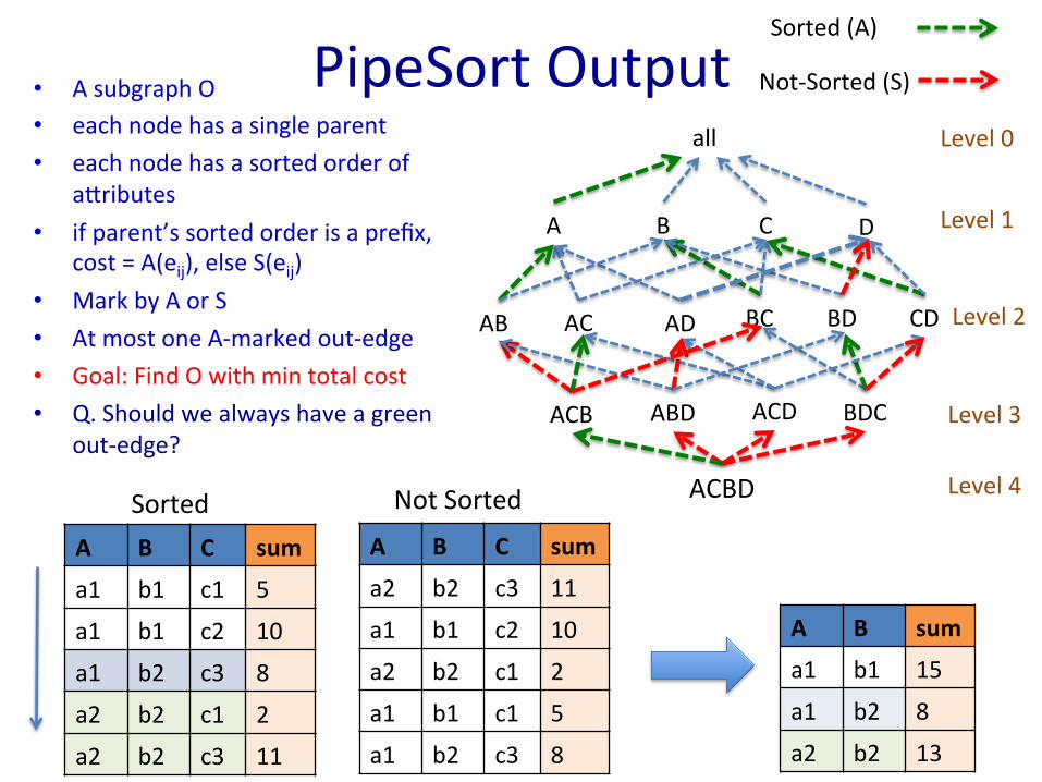
PipeSort Output • A subgraph O • each node has a single parent • each node has a sorted order of
ahributes • if parent’s sorted order is a prefix,
cost = A(eij), else S(eij) • Mark by A or S • At most one A-‐marked out-‐edge • Goal: Find O with min total cost • Q. Should we always have a green
out-‐edge?
ACBD
ACB ABD ACD BDC
AC AD BC BD CD AB
A B C D
all Level 0
Level 1
Level 2
Level 3
Level 4
A B C sum
a1 b1 c1 5
a1 b1 c2 10
a1 b2 c3 8
a2 b2 c1 2
a2 b2 c3 11
Not Sorted
A B C sum
a2 b2 c3 11
a1 b1 c2 10
a2 b2 c1 2
a1 b1 c1 5
a1 b2 c3 8
Sorted
A B sum
a1 b1 15
a1 b2 8
a2 b2 13
Sorted (A)
Not-‐Sorted (S)

Outline: PipeSort Algorithm (1) • Go from level 0 to N-‐1
– here N = 4
• For each level k – find the best way to construct it from level k+1
• Weighted Bipar>te Matching – G(V1, V2, E) – Weight on edges – each vertex in V1 should be connected to at most one vertex in V2 – Find a matching of max total weight – Here min total weight – w -‐> max_weight – w – Requires |V2| >= |V1|
ABCD
ABC ABD ACD BCD
AC AD BC BD CD AB
A B C D
all Level 0
Level 1
Level 2
Level 3
Level 4

Outline: PipeSort Algorithm (2) • Reduc>on to a weighted
bipar>te matching between level k and k+1
• Make k new copies of each node in level k+1
– k+1 copies for each in total – replicate edges
• Original copy = cost A(eij) = sorted
– sorted order of i fixed
• New copies = cost S(eij) = not sorted
– need to sort i
ABCD
ABC ABD ACD BCD
AC AD BC BD CD AB
A B C D
all Level 0
Level 1
Level 2
Level 3
Level 4
Make new 2 copies Total 3 copies each
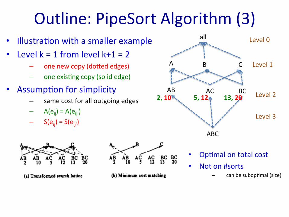
Outline: PipeSort Algorithm (3) • Illustra>on with a smaller example • Level k = 1 from level k+1 = 2
– one new copy (dohed edges) – one exis>ng copy (solid edge)
• Assump>on for simplicity – same cost for all outgoing edges – A(eij) = A(eij’) – S(eij) = S(eij’)
ABC
AC BC AB
A B C
all Level 0
Level 1
Level 2
Level 3
2, 10 5, 12 13, 20
• Op>mal on total cost • Not on #sorts
– can be subop>mal (size)

Azer compu>ng the plan, execute all pipelines
Outline: PipeSort Algorithm (4)
1. First pipeline is executed by one scan of the data
2. Sort CBAD -‐> BADC, compute the second pipeline
3. …..
A, S costs

Observa>ons: • Finds the best plan for compu>ng level k
from level k+1 – Assuming the cost of sor>ng “BAD” does not depend on how the GROUP-‐BY on “BAD” has been computed
• Genera>ng plan k+1 -‐> k does not prevent genera>ng plan k+2 -‐> k+1 from finding the best choice
• Not provably globally op>mal – e.g. can the op>mal plan compute AB from ABCD? – something to explore!
Outline: PipeSort Algorithm (5)
ABCD
ABC -‐> BCA
BC
If the green edge is chosen, the sorted order of ABCD will be BCAD

PipeHash Algorithm
31

• Use hash tables to compute smaller GROUP-‐BYs
• If the hash tables for AB and AC fit in memory, compute both in one scan of ABC
• With no memory restric>ons
for k = N...0: For each k+1-‐ahribute GROUP BY g Compute in one scan of g all k-‐ahribute GROUP
BY where g is smallest parent Save g to disk and destroy the hash table of g
ABCD
ABC ABD ACD BCD
AC AD BC BD CD AB
A B C D
all
PipeHash: Basic Idea (1) N = 4
A B sum
a1 b1 15
a1 b2 8
a2 b2 13
A B C sum
a1 b1 c1 5
a1 b1 c2 10
a2 b2 c3 8
a2 b2 c1 2
a2 b2 c3 11
A C sum
a1 c1 5
a1 c2 10
a2 c3 19
a2 c1 2

• But, data might be large, Hash Tables may not fit in memory
• Solu>on: op>miza>on “shared-‐par>>on” – par>>on data on one or more ahributes – Suppose the data is par>>oned on ahribute A – All GROUP-‐Bys containing A (AB, AC, AD, ABC…) can be computed independently on each par>>on – Cost of par>>oning is shared by mul>ple GROUP-‐BYs
ABCD
ABC ABD ACD BCD
AC AD BC BD CD AB
A B C D
all
PipeHash: Basic Idea (2) N = 4
A B sum
a1 b1 15
a1 b2 8
a2 b2 13
A B C sum
a1 b1 c1 5
a1 b1 c2 10
a2 b2 c3 8
a2 b2 c1 2
a2 b2 c3 11
A C sum
a1 c1 5
a1 c2 10
a2 c3 19
a2 c1 2

• Input: search latce • For each group-‐by, select smallest parent • Result: Minimum Spanning Tree (MST)
ABCD
ABC ABD ACD BCD
AC AD BC BD CD
A B C D
all
N = 4
AB
Size of GROUP-BY
• But, all Hash Tables (HT) in the MST may not fit in the memory together
• To consider: – Which GROUP-‐BYs to compute together? – When to allocate-‐release memory for HT? – What ahributes to par>>on on?
PipeHash: Basic Idea (3)

• Once again, a combinatorial op>miza>on problem • This problem is conjectured to be NP-‐complete in the paper
– something to explore!
• Use heuris>cs
Outline: PipeHash Algorithm (1)
Trade-‐offs 1. Choose as large sub-‐tree of MST as possible (“cache-‐results”, “amor>zed
scan”) 2. The sub-‐tree must include the par>>oning ahribute(s)
Heuris>c Choose a par>>oning ahribute that allows selec>on of the largest subtree of MST

Algorithm • Input: search latce • worklist = {MST} • while worklist not empty
• select one tree T from the worklist • T’ = select-‐subtree(T) • Compute-‐subtree(T’)
Next, through examples • Select-‐subtree(T)
– May add more subtrees to worklist
• Compute-‐subtree(T’)
ABCD
ABC ABD ACD BCD
AC AD BC BD CD
A B C D
all
AB
Outline: PipeHash Algorithm (2)
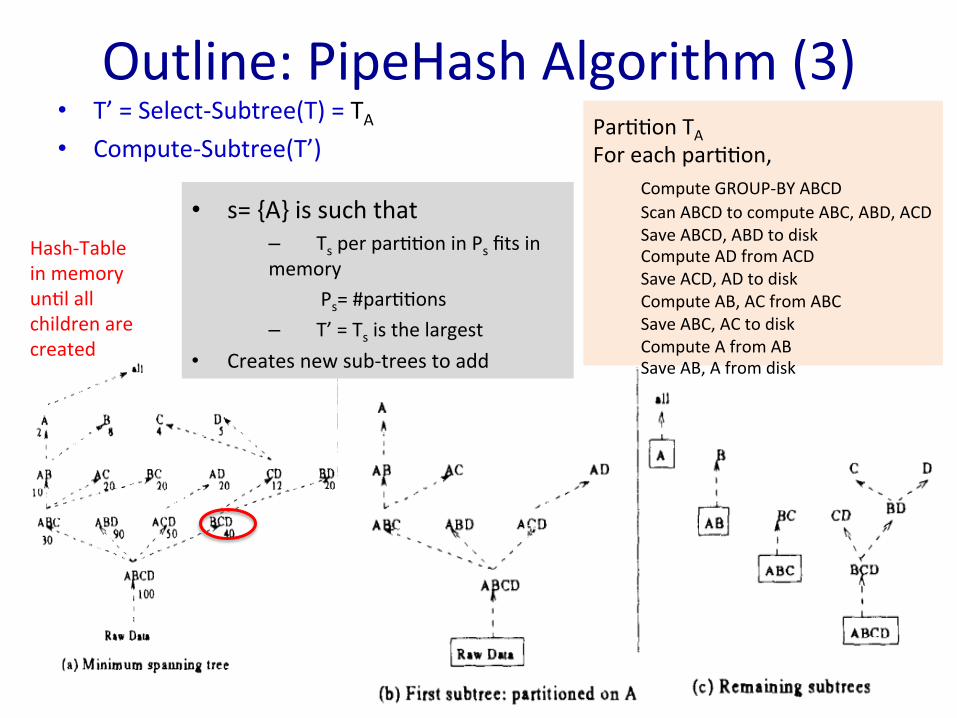
• T’ = Select-‐Subtree(T) = TA • Compute-‐Subtree(T’)
Outline: PipeHash Algorithm (3)
• s= {A} is such that – Ts per par>>on in Ps fits in memory
Ps= #par>>ons – T’ = Ts is the largest
• Creates new sub-‐trees to add
Par>>on TA For each par>>on,
Compute GROUP-‐BY ABCD Scan ABCD to compute ABC, ABD, ACD Save ABCD, ABD to disk Compute AD from ACD Save ACD, AD to disk Compute AB, AC from ABC Save ABC, AC to disk Compute A from AB Save AB, A from disk
Hash-‐Table in memory un>l all children are created

Experiments
• Here sort-‐based beher than hash-‐based (new hash-‐table for each GROUP-‐BY)
• Another experiment on synthe>c data (see paper) • For less sparse data, hash-‐based beher than sort-‐based

Summary • Similar Overlap algorithm by Deshpande et al. (see
paper)
• All algorithms try to pick the best plan to compute aggregates with fewer scans and maximal memory usage • Finding op>mal decisions for each algorithm may be NP-‐
complete • Algorithms use heuris>cs that work well in prac>ce
• Next class: other efficient implementa>ons and index for cube