Embed Size (px)
Citation preview

DOI: 10.1007/s004539910019
Algorithmica (2000) 26: 389–429 Algorithmica© 2000 Springer-Verlag New York Inc.
Algorithms for Sensorless Manipulation Using aVibrating Surface1
K.-F. Bohringer,2 V. Bhatt,3 B. R. Donald,4 and K. Goldberg5
Abstract. We describe a programmable apparatus that uses a vibrating surface for sensorless, nonprehensilemanipulation, where parts are systematically positioned and oriented without sensor feedback or force closure.The idea is to generate and change the dynamic modes of a vibrating surface. Depending on the node shapesof the surface, the position and orientation of the parts can be predicted and constrained. The vibrating surfacecreates a two-dimensional force vector field. By chaining together sequences of force fields, the equilibriumstates of a part in the field can be successively reduced to obtain a desired final state. We describe efficientpolynomial-time algorithms that generate sequences of force fields for sensorless positioning and orientingof planar parts, and we show that these strategies are complete. Finally we consider parts feeders that canonly implement a finite set of force fields. We show how to plan and execute strategies for these devices. Wegive numerical examples and experiments. and discuss tradeoffs between mechanical complexity and planningcomplexity.
Key Words. Vibratory parts feeders, Sensorless manipulation, Nonprehensile manipulation, Programmableforce fields, Open-loop positioning and orienting, Industrial parts feeding.
1. Introduction. It is often extremely costly to maintain part order throughout themanufacture cycle. For example, instead of keeping parts in pallets, they are often de-livered in bags or boxes, whence they must be picked out and sorted. A parts feeder isa machine that orients such parts before they are fed to an assembly station. Currently,the design of parts feeders is a black art that is responsible for up to 30% of the costand 50% of workcell failures [43], [13], [27], [54], [55].“The real problem is not parttransfer but part orientation,” Frank Riley, Bodine Corporation [52, p. 316, his italics].Thus although part feeding accounts for a large portion of assembly cost, there is notmuch scientific basis for automating the process.
The most common type of parts feeder is thevibratory bowl feeder, where parts ina bowl are vibrated using a rotary motion, so that they climb a helical track. As theyclimb, a sequence of baffles and cutouts in the track create a mechanical “filter” that
1 A brief preliminary version of this paper was presented at the International Conference on Robotics and Au-tomation (Nagoya, Japan, April 1995). Karl B¨ohringer received support from the National Science Foundationunder a Postdoctoral Associateship CDA-9726389 and a CAREER award ECS-9875367. Support for BruceDonald was provided by the NSF under Grant Nos. IRI-8802390, IRI-9000532, IRI-9201699, NSF/DARPAIRI-9403903, IRI-9530785, CDA-9726389, 9802068, CISE/CDA-9805548, EIA-9818299, IRI-9896020, EIA-9901407, IIS-9906790, and by the AFOSR, the Mathematical Sciences Institute, Intel Corporation, AT&T Belllaboratories, and an equipment grant from Microsoft Research.2 Department of Electrical Engineering, University of Washington, Seattle, WA 98195-2500, USA.3 GE Medical Systems, Milwaukee, WI 53219, USA.4 Department of Computer Science, Dartmouth College, Hanover, NH 03755-3510, USA.5 Department of Industrial Engineering and Operations Research, University of California, Berkeley, CA94720-1777, USA.
Received November 15, 1996; revised January 18, 1998. Communicated by R. Motwani and P. Raghavan.

390 K.-F. Bohringer, V. Bhatt, B. R. Donald, and K. Goldberg
causes parts in all but one orientation to fall back into the bowl for another attempt atrunning the gauntlet [13], [52], [53]. To improve feed rate, it is sometimes possible todesign the track so as to rotate parts mechanically into a desired orientation (this is calledconversion). Related methods use centrifugal forces [27], reciprocating forks, or belts tomove parts through the filter [49].
Sony’s APOS parts feeder [32] uses an array of nests (silhouette traps) cut into avibrating plate. The nests and the vibratory motion are designed so that the part willremain in the nest only in one particular orientation. By tilting the plate and letting partsflow across it, the nests eventually fill up with parts in the desired orientation. Althoughthe vibratory motion is under software control, specialized mechanical nests must bedesigned for each part [42].
The reason for the success of vibratory bowl feeders and the Sony APOS system is theunderlying principle ofsensorless manipulation[25] that allows parts positioning andorienting without sensor feedback. The theory of sensorless manipulation is the sciencebase for developing and controlling such devices.
Despite their popularity, all vibratory feeders mentioned so far have some disadvan-tages:
1. Parts may get wedged or entangled in filters.2. Parts may get damaged when dropping back into the bowl, or worn by repeated
rejections.3. Each filter reduces the feed rate, depending on the ratio between rejected and accepted
parts.4. The filters must be redesigned for each new part geometry, a task that usually requires
skilled work by human experts.6
In the early 1980s several researchers used sensors to determine the pose of partsdelivered by a vibratory track [49]. Sensors such as tactile probes [29], [35], photocells[30], fiber-optic sensors [44], and machine vision systems [31], [56] were employed.Once part pose was determined, air-jets and trapdoors were used to group parts in similarposes.
Singer and Seering [55] proposed several designs for parts feeders where programmedvibration was used to drive parts into a stable configuration. Their methods can be usefulfor bringing parts into one of several poses where its center of mass is as low as possible.Swanson et al. [57] and Tran et al. [59] used vibrating surfaces for parts feeding strategies,and achieved dynamic equilibrium states to pose parts.
In this paper we explore how controlled vibration can be used for a new setup to feedplanar parts systematically (i.e., parts with extruded polygonal shapes and low aspect-ratio). The idea is to generate and change dynamic modes in a plate by varying appliedfrequencies. Depending on the frequency of vibration and the boundary conditions, nodesof different shapes are formed. If planar parts are put on this vibrating plate, they moveto the node, and end up in a stable orientation [5]. We develop an analysis wherebygiven the shape of the node, and the part geometry, the final orientation can be predicted.For our device, we further propose a “sensorless” strategy for part manipulation [25],
6 Caine [15] presented an experimental CAD system that assists the construction of track filters for vibratorybowl feeders.

Algorithms for Sensorless Manipulation Using a Vibrating Surface 391
building on the theory originally developed for feeding parts using parallel-jaw grippers[28], which was recently extended to arrays of microactuators and programmable forcefields [9], [8].
Note that manipulation with force fields is a form of nonprehensile manipulation [22],[60], [26], [24], [17]: parts are manipulated without form or force closure.
In robotics,minimalism[16], [6] has become increasingly influential. Minimalismbegins with the proposition that doing task A without resource B is interesting, becausedoing so proves that B is somehow inessential to the information structure of the task.Thus, minimalism attempts to reduce the resource signature [6] for a task. Taking the“transitive closure” of this proposition would result in finding the minimal configurationof resources required to solve a task. Raibert [46] showed that running machines couldbe built without static stability. Erdmann and Mason [25] showed how to do dextrousmanipulation without sensing. McGeer [40] built a biped, kneed walker without sensors,computers, or actuators. Brooks [14] has developed on-line algorithms that rely lessextensively on planning and world models. Canny and Goldberg [16] have demonstraterobot systems of minimal complexity. Donald et al. [22], [6] have built distributed teamsof mobile robots that cooperate in manipulation without explicit communication. Themanipulation algorithms presented in this paper attempt to minimize the sensor inputand the required hardware.
Our results on equilibrium analysis, planning and manipulation strategies, and com-putational complexity devolve to an application of the theory of programmable forcefields introduced by B¨ohringer et al. [8]. This paper applies their algorithmic frameworkto a new class of vibratory devices. The main characteristics of our device are:
• simple design, with no mechanical filters (addressing disadvantages 1–3),• programmability (addressing problem 4).
Section 2 gives an overview on our research agenda, from the basic ideas of sensor-less manipulation using programmable force fields, to the use of discrete force fields.Section 3 describes the design of our devices, and the performed experiments. It alsopresents a device that can implement a particularly useful class of fields called squeezefields. In Section 4 we first investigate the dynamics of small particles on the plate, todeduce the approximate nature of the effective force field generated by the vibratingplate. Then we discuss the dynamic behavior of planar objects in such a force field. InSection 5 this model is used to predict the stable rest configurations (equilibria) for partson the vibrating plate, and the predictions are compared with experimental results. Basedon these results, we develop manipulation strategies with squeeze fields that uniquelyorient objects. However, not all vibratory devices can generate arbitrary squeeze fields.Section 6 presents new algorithms that use only limited sets of fields, and introducesmanipulation grammars. We demonstrate how they can be used to program our devicefor sensorless manipulation tasks. We close by giving an outlook on future work andopen problems.
2. A Science Base for Vibratory Manipulation. In a programmable force field, theforces generated at each point of the field can be controlled independently. Programmableforce fields can be used to control a variety of flexible planar parts feeders. These devices

392 K.-F. Bohringer, V. Bhatt, B. R. Donald, and K. Goldberg
Fig. 1. Sensorless parts orienting using programmable force fields: the part reaches unique orienta-tion after two subsequent squeezes. There exist such orientating strategies for all polygonal parts. Seewww.cs.dartmouth.edu/˜brd/demo/VibratoryAlign for an animated simulation.
can exploit exotic actuation technologies such as arrayed, microfabricated motion pixels[9] or, in the case of this paper, transversely vibrating plates. These new automationdesigns promise great flexibility, speed, and dexterity—they may be employed to orient,singulate, sort, feed, and assemble parts (see, for example, Figures 1 and 8). However,since they have only recently been invented, programming and controlling them formanipulation tasks is challenging. Our research goal is to develop a science base formanipulation using programmable force fields.
Since the eighteenth century scientists have studied vibrating plates, which causeparticles on the plate to arrange along vibratory nodes in so-called Chladni7 figures [18].These nodes in the force fields depend to a large extent on the vibration frequency, andon the location of clamped and free plate edges. Hence by changing the input frequency,or adding software-controlled clamps, specific force fields can be generated.
When a part is placed on our devices, the programmed force field induces a forceand moment upon it. Over time, the part may come to rest in a dynamic equilibriumstate. In principle, we have tremendous flexibility in choosing the force field, since using
7 After the German physicist Ernst Chladni, 1756–1827, whose objective was a schematic approach to theconstruction of better musical instruments.

Algorithms for Sensorless Manipulation Using a Vibrating Surface 393
software-controlled vibratory devices, the force field may be programmed in a fairly fine-grained fashion. Hence, we have a lot of control over the resulting equilibrium states.By chaining together sequences of force fields, the equilibria may be cascaded to obtaina desired final state—for example, this state may represent a unique orientation or poseof the part. A system with such a behavior exhibits thefeeding property[1]:
A system has thefeeding propertyover a set of partsP and a set of initial configu-rationsI if, given any partP ∈ P, there is some output configurationq such thatthe system can moveP to q from any location inI.
This paper first describes our experimental devices and a technique for analyzingthem calledequilibrium analysis. Then we describe new manipulation algorithms usingthese tools, and we relax earlier dynamic and mechanical assumptions to obtain morerobust and flexible strategies.
2.1. From Continuous Squeeze Fields to Discrete Manipulation Grammars
2.1.1. Sensorless Manipulation Using Continuous Squeeze Fields. We develop our re-sults as follows: In order to discuss planning and control algorithms for the vibrating platedevice, first, we make some idealizing assumptions about the kinds of fields it can imple-ment. In particular, we initially assume that it can implement a continuum of “squeezefields.” Next, we further develop a particular simplified dynamic model, called 2PHASE,in which translation and rotation are essentially “decoupled.” We then carefully definethe computational problem of synthesizing control strategies guaranteed to orient a partfrom any initial configuration. We find that motion plans with a simple structure suffice.
With current vibratory devices, the rich “vocabulary” required for this idealized modelis not attainable. Therefore, we show how our approach generalizes to the practicallimitations of our devices, and, in the process, relax our assumptions to include a morerealistic dynamic model.
2.1.2. Generalizing to Discrete Manipulation Grammars. We now make the researchagenda of Section 2.1.1 precise, and give the reader an overview of our technical results.Previous results on array and force field manipulation strategies may be formalized us-ing equilibrium analysis. In [10] Bohringer et al. proposed a family of control strategiescalledsqueeze fieldsand a planning algorithm for parts orientation. This first result provedan O(n2) upper bound on the numberE of orientation equilibria of a nonpathological(see Section 5.1) planar part withn vertices. This yields anO(E2) = O(n4) planningalgorithm to orient a part uniquely, under certain geometric, dynamic, and mechanicalassumptions. The strategies employed by these algorithms require significant mechani-cal and control complexity—even though they require no sensing. The requisite degreeof controllability does not exist yet for vibrating plates. For this reason, we introduceand analyze strategies composed of field sequences that we know are implementableusing current vibrating plate technology. Each strategy is a sequence of pairs of squeezessatisfying certain “orthogonality” properties. Under these assumptions, we can ensure
(a) equilibrium stability,(b) general first-order dynamics and simple force fields, and(c) complexity and completeness guarantees.

394 K.-F. Bohringer, V. Bhatt, B. R. Donald, and K. Goldberg
The framework is quite general, and applies to any set of primitive operations satis-fying certain “finite equilibrium” properties—hence it has broad applicability to a widerange of devices. In particular, we view the restricted class of fields as avocabularyand their rules of composition as agrammar, resulting in a “language” of manipulationstrategies.
Finally, our finitemanipulation grammarhas the following advantage over previousmanipulation algorithms for programmable force fields: previous algorithms such asthose described in [9] guarantee to orient a part uniquely, but the translational positionof the part is unknown at the strategy’s termination. Our new algorithms guarantee toposition the part uniquely (up to part symmetry) in translationas well asorientationspace. Like the algorithms in [9] and [8], the new algorithms require no sensing, andwork from any initial configuration to uniquely pose the part. In particular, the initialconfiguration is never known to the (sensorless) execution system, which functions open-loop.
The complexity and completeness guarantees we obtain for manipulation grammarsare weaker than for the general squeeze field strategies. For squeeze strategies, we applythe algorithmic theory of [8] to show thatany nonpathological planar part with finitearea contact can be placed in a unique orientation inO(E) = O(n2) steps. Under themanipulation grammar, our planner is guaranteed to find a strategy if one exists (if onedoes not exist, the planner will signal this). However, it is not known whether there existsa strategy for every part. This lack of completeness of manipulation grammar strategiesstands in contrast to thecompletealgorithms of [9] and [8] for which aguaranteedstrategy exists forall parts. Moreover, the planning algorithm is worst-case exponentialinstead of merely quadratic in the number of vertices of the part.
3. Experimental Observations
3.1. Setup and Calibration. Figures 2 and 3 are schematics of the experimental setup,which consists of an aluminum plate forced to oscillate in two different configurations.The shaker is a commercially available8 electrodynamic vibration generator, with a
Fig. 2.Schematic of experimental setup 1: a 50 cm× 40 cm aluminum plate is forced to oscillate horizontallyby the shaker armature. The forced oscillation causes a transverse vibration of the plate.
8 Model VT-100G, Vibration Test Systems, Akron, OH, USA.

Algorithms for Sensorless Manipulation Using a Vibrating Surface 395
Fig. 3.Schematic of experimental setup 2: the aluminum plate is hinged and can oscillate about an axis in itsmiddle.
linear travel of 0.02 m, and capable of producing a force of up to 500 N. The inputsignal, specifying the waveform corresponding to the desired oscillations, is fed to asingle coil armature, which moves in a constant field produced by a ceramic permanentmagnet in a center gap configuration.
In the first configuration (Figure 2), the plate is attached to the shaker armature suchthat it is forced to vibrate in the longitudinal direction (i.e., along the plate axis). For lowamplitudes and frequencies, the plate moves with no perceptible transverse vibrations(i.e., vibrations perpendicular to the plate). However, as the frequency of oscillationsis increased, transverse vibrations of the plate become more pronounced. The resultingmotion is similar to the forced transverse vibration of a rectangular plate, clamped onone edge and free along the other three sides.
The nodes for these transverse oscillations can either be obtained theoretically [48],[58], or experimentally using the technique originally pioneered by Chladni [18]. Bysprinkling small sized particles9 on a vibrating surface, the nodes can be experimentallyidentified as the regions where the particles tend to collect. The dynamics of “collecting”at the nodes is important in determining the effective force field that leads to the orientingand localization effect of our device, and is discussed in more detail in Section 4.
For the configuration in Figure 2, the location and shape of the node depends onthe frequency of vibration. Figure 4 shows experiments to determine the nodes forfrequencies of 60 Hz and 100 Hz.
The second configuration (Figure 3) forces the plate to undergo transverse vibrationssuch that the resulting shape of the node, and its location, are independent of the forcingfrequency. The plate is hinged about an axis situated midway between, and parallelto, two of its sides. A rod connected to the armature of the shaker forces the plate toan oscillatory motion about the hinged axis. As expected, experimental determinationshows that except for a slight distortion due to the effect of clamping at the rod, the nodelines up with the hinge axis (Figure 5).
9 Chladni used sand, we use Urad lentils to get a better contrast.

396 K.-F. Bohringer, V. Bhatt, B. R. Donald, and K. Goldberg
Fig. 4.Experimentally determined nodes at (a) 60 Hz and (b) 100 Hz, for experimental setup 1 (see Figure 2).After vibrating the plate for a short time, the particles form Chladni figures, which indicate the location of thevibrational nodes.
The second setup is run at lower frequencies, to ensure that only the mode where theplate oscillates about the hinge axis is excited. If we increase the operating frequency,modes corresponding to transverse vibration of a plate, clamped at the point of attachmentto the rod and the hinged ends, become dominant, and the node shape gets complicated.This effect can be seen at 20 Hz (Figure 5), where the node shows a tendency to get“pulled” toward the point where the plate is clamped to the rod.
3.2. Behavior of Planar Parts. If we put planar parts on the vibrating surface, thereis a marked tendency for them to move toward the node and end up in one of a finitenumber of stable orientations. We observe the following features over a wide range offrequencies in both the experimental setups:
• From all initial positions on the plate, the objects move towards the node. They endup in a stable position around some point on the node, which depends on the initialposition of the object.• As the object approaches the node (as we show later, after some portion of it crosses
the node), there is a tendency for it to rotate until it reaches one of a finite number ofstable orientations.
Fig. 5.Experimentally determined vibrational nodes at (a) 10 Hz and (b) 20 Hz, for experimental setup 2 (seeFigure 3).

Algorithms for Sensorless Manipulation Using a Vibrating Surface 397
Fig. 6. Stable position of planar parts in experimental setup 1, at a frequency of 60 Hz. The node is markedaccording to Figure 4.
Figure 6 shows two planar shapes, a triangle and a trapezoid, after they have reachedtheir stable position and orientation for the setup in Figure 2. To illustrate the orientingeffect better, the curve showing the node has been drawn by hand. Figure 7 similarlyshows the stable position of the planar parts for the second setup.
Over the large number of experimental runs performed, there are a couple of quali-tative observations describing the ease and speed with which the parts get into a stableconfiguration:
• At higher frequencies of oscillation, both the velocity of the part toward the node, andthe rate of orientation, are relatively faster.• Objects with a higher degree of rotational asymmetry get into a stable orientation
more easily.
Although the location of the node is better identified in the second setup, the loweroperating frequencies make the localization of the part at the node, and the correspondingorienting behavior, much slower.
Fig. 7. Stable position of planar parts in experimental setup 2, at a frequency of 20 Hz. The node is markedaccording to Figure 5.

398 K.-F. Bohringer, V. Bhatt, B. R. Donald, and K. Goldberg
4. Dynamics of Particles and Planar Parts on a Vibrating Plate. The underlyingdynamics that causes the objects placed on a vibrating surface to move toward the nodegive rise to an effective force field. In order to develop a theory for using our device as aviable method for sensorless manipulation, it is important to determine the genesis andvariation of this force field over the vibrating plate.
4.1. Chladni Figures. When particles are spread on a vibrating surface, they collectat the nodes, resulting in patterns known as Chladni figures (after Chladni [18], seeFigures 4 and 5). Rayleigh [48] describes the motion of the particles toward the nodesin the following words: “the movement to the nodes is irregular in its character. If agrain be situated elsewhere than at a node, it is made to jump by a sufficiently vigoroustransverse vibration. The result may be a movement either towards or from a node; butafter a succession of such jumps the grain ultimately finds its way to a node.”
The forces that cause the particles to move to the node act on any object placed on thevibrating surface, generating an effective force field. The underlying dynamics of thisphenomenon are very complex. In Appendix A we give an approach toward an analyticalmodel for the more tractable case of the planar motion of a particle bouncing on a stringin transverse vibration.
4.2. Motion and Equilibria of Planar Parts. The case of general large objects on theplate is more complicated than individual particles, because the determination of thepoints on the object that undergo impact, and the resulting impulses, are both difficultproblems to solve. For our analysis, we ignore effects such as rolling and tilting of theparts and assume that the contact geometry remains constant over the impacts.
We can consider the planar parts as a rigid arrangement of “particles,” each of whichinteracts with the plate and experiences the effective force field discussed in Section 4.1.The forces have to be summed up over the area of contact, giving a specific force (perunit area),f , that acts at every point of the planar object.
Let P be the planar part in contact with the vibrating plate, and letc denote thecenter of area ofP. The total net forcefP and momentMP aroundc can be obtained byintegrating the force fieldf over the contact surface ofP:
fP =∫
Pf d A,(1)
MP =∫
P(r − c)× f d A.(2)
Consider a partP on the vibrating plate. We assume that a first-order dynamicalsystem describes the motion ofP on the plate. In a first-order system, the velocity of apart is directly proportional to the force acting on it. Hence, anequilibriumis a placementof P such thatP remains stationary. In an equilibrium, the force and moment acting onP are balanced. Thisequilibrium conditionis met when the net forcefP and momentMP ((1) and (2)) are both zero.
We have made a series of assumptions to suggest that a force field exists for partson a planar plate. Our experimental results indicate that they are good engineeringassumptions when we observe the system over time, due to an averaging effect causedby the vibration of the plate. An “exact” modeling of the impact dynamics between

Algorithms for Sensorless Manipulation Using a Vibrating Surface 399
Fig. 8. Sensorless sorting using programmable force fields: parts of different sizes are first centered andsubsequently separated depending on their size.
part and plate, even though possible (see, e.g., [41] and [50]), is not necessary for ourpurposes.
5. Equilibrium Analysis for Programmable Force Fields. For the generation ofmanipulation strategies with programmable force fields it is essential to be able to pre-dict the motion of a part in the field. Particularly important is determining the stableequilibrium poses a part can reach in which all forces and moments are balanced. Thisequilibrium analysiswas introduced in [10], where B¨ohringer et al. presented a theoryof manipulation for programmable force fields, and an algorithm that generates manip-ulation strategies to orient polygonal parts without sensor feedback using a sequence ofsqueeze fields. We now briefly review their algorithm and its complexity bounds.
5.1. Squeeze Fields and Equilibria. In [10] Bohringer et al. proposed a family ofcontrol strategies calledsqueeze fieldsand a planning algorithm for parts orientation.
DEFINITION 1. Assumel is a straight line through the origin. Asqueeze field fis atwo-dimensional force field defined as follows:
1. If z ∈ R2 lies onl , then f (z) = 0.2. If z does not lie onl , then f (z) is the unit vector normal tol and pointing towardl .

400 K.-F. Bohringer, V. Bhatt, B. R. Donald, and K. Goldberg
Fig. 9.Equilibrium condition: to balance force and moment acting onP in a unit squeeze field, the two areasP1 andP2 must be equal (i.e.,l must be a bisector), and the line connecting the centers of areac1 andc2 mustbe perpendicular to the node line.
We refer to the linel as thesqueeze line, becausel lies in the center of the squeezefield.
Assuming quasi-static motion, an object will move perpendicularly toward the linel and come to rest there. We are interested in the motion of an arbitrarily shaped (notnecessarily small) partP. We call P1, P2 the regions ofP that lie to the left and to theright of l , respectively, andc1, c2 their centers of area. In a rest position both translationaland rotational forces must be in equilibrium. We obtain the following two conditions:
I. The areasP1 andP2 must be equal.II. The vectorc2− c1 must be normal tol .
P has a translational motion component normal tol if I does not hold.P has a rotationalmotion component ifII does not hold (see Figure 9). This assumes a uniform forcedistribution over the surface ofP, which is a reasonable assumption for planar parts insurface contact.
DEFINITION 2. A part P is in translational equilibriumif the forces acting onP arebalanced.P is in orientational equilibriumif the moments acting onP are balanced.Total equilibriumis simultaneous translational and orientational equilibrium.
Let (x0, y0, θ0) be an equilibrium pose ofP. (x0, y0) is the correspondingtranslationequilibrium, andθ0 is the correspondingorientation equilibrium.
DEFINITION 3. A bisectorof a polygonP is a line that cutsP into two regions of equalarea.
PROPOSITION4. Let P be a polygon whose interior is connected.There exist O(k n2)bi-sectors such that P is in equilibrium when placed in a squeeze field such that the bisectorcoincides with the squeeze line. n is the part complexity measured as the number of poly-gon vertices. k denotes the maximum number of polygon edges that a bisector can cross.
If P is convex, then the number of bisectors is bounded by O(n).

Algorithms for Sensorless Manipulation Using a Vibrating Surface 401
This proposition constitutes a key result for the complexity analysis of manipulationstrategies with programmable force fields. Several results in this paper are based on thebounds summarized in Proposition 4. Its proof can be found in Appendix B. For mostpart geometries,k is a small constant.10 However, in the worst case, pathological partscan reachk = O(n). A (e.g., rectilinear) spiral-shaped part would be an example forsuch a pathological case, because every bisector intersectsO(n) polygon edges.
5.2. Planning of Manipulation Strategies. In this section we present an algorithm forsensorless parts alignment with squeeze fields [9], [8]. Recall from Section 5.1 that insqueeze fields, the equilibria for connected polygons are discrete (modulo a neutrallystable translation parallel to the squeeze line which we will disregard for the remainderof Section 5).
To model actuator arrays and vibratory devices, the following assumptions are made:
DENSITY: The generated forces can be described by a vector field.2PHASE: The motion of a part has two phases: (1) Pure translation towardl until the part is
in translational equilibrium. (2) Motion in translational equilibrium until orientationalequilibrium is reached.
Note that due to the elasticity and oscillation of the actuator surfaces, we can assumecontinuous area contact, and not just contact in three or a few points. If a part moveswhile in translational equilibrium, in general the motion is not a pure rotation, but alsohas a translational component. Therefore, relaxing assumption 2PHASE is one of the keyresults of this paper.
DEFINITION 5. Let θ be the orientation of a connected polygonP in a squeeze field,and let us assume that conditionI holds. Theturn function t: θ → {−1,0,1} describesthe instantaneous rotational motion ofP:
t (θ) = 1 if P will turn counterclockwise,−1 if P will turn clockwise,
0 if P is in total equilibrium (Figure 10).
See Figure 10 for an illustration. The turn functiont (θ) can be obtained, for example,by taking the sign of the lifted momentMP(z) for posesz= (x, y, θ) in which the liftedforce fP(z) is zero.
Definition 5 immediately implies the following lemma:
LEMMA 6. Let P be a polygon with orientationθ in a squeeze field such that conditionI holds. P is stable if t(θ) = 0, t (θ+) ≤ 0, and t(θ−) ≥ 0. Otherwise P is unstable.
PROOF. Assume the partP is in a pose(x, y, θ) such that conditionI is satisfied. Thisimplies that the translational forces acting onP balance out. If in additiont (θ) = 0,then the effective moment is zero, andP is in total equilibrium. Now consider a smallperturbationδθ > 0 of the orientationθ of P while conditionI is still satisfied. For a
10 In particular, in [10] we assumed thatk = O(1).

402 K.-F. Bohringer, V. Bhatt, B. R. Donald, and K. Goldberg
Fig. 10. (a) Polygonal part. Stable (thick line) and unstable (thin line) bisectors are also shown. (b) Momentfunction. (c) Turn function, which predicts the orientations of the stable and unstable bisectors. (d) Squeezefunction, constructed from the turn function. (e) Alignment strategy for two arbitrary initial configurations.
stable equilibrium, the moment resulting from the perturbationδθ must not aggravatebut rather counteract the perturbation. This is true if and only ift (θ + δθ ) ≤ 0 andt (θ − δθ ) ≥ 0.
Using this lemma we can identify all stable orientations, which allows us to constructthe squeeze function [28] ofP (see Figure 10(d)), i.e., the mapping from an initialorientation ofP to the stable equilibrium orientation that it will reach in the squeezefield:
LEMMA 7. Let P be a polygonal part on an actuator arrayA such that assumptionsDENSITY and2PHASE hold. Given the turn function t of P, its correspondingsqueezefunctions: S1→ S1 is constructed as follows:
1. All stable equilibrium orientationsθ map identically toθ .2. All unstable equilibrium orientations map(by convention) to the nearest counter-
clockwise stable orientation.3. All orientationsθ with t(θ) = 1 (−1)map to the nearest counterclockwise(clockwise)
stable orientation.
Then s describes the orientation transition of P induced byA.

Algorithms for Sensorless Manipulation Using a Vibrating Surface 403
PROOF. Assume that partP initially is in pose(x, y, θ) in arrayA. Because of 2PHASE,we can assume thatP translates toward the center linel until condition I is satisfiedwithout changing its orientationθ . P will change its orientation until the moment iszero, i.e.,t = 0: a positive moment (t > 0) causes counterclockwise motion, and anegative moment (t < 0) causes clockwise motion until the next root oft is reached.
We conclude that any connected polygonal part, when put in a squeeze field, reachesone of afinite number of possible orientation equilibria [9], [8]. The motion of the partand, in particular, the mapping between initial orientation and equilibrium orientation isdescribed by the squeeze function, which is derived from the turn function as describedin Lemma 7. Note that all squeeze functions derived from turn functions are monotonestep-shaped functions.
Goldberg [28] has given an algorithm that automatically synthesizes a manipulationstrategy to orient a part uniquely, given its squeeze function. While Goldberg’s algorithmwas designed for squeezes with a robotic parallel-jaw gripper, in fact, it is more general,and can be used for arbitrary monotone step-shaped squeeze functions. The output ofGoldberg’s algorithm is a sequence of angles that specify the required directions of thesqueezes. Hence these angles specify the direction of the squeeze line in our force fields(for example the two-step strategy in Figure 10(e)).
It is important to note that the equilibria obtained by a force field and by a parallel-jaw gripper will typically be different, even when the squeeze directions are identical.For example, consider squeezing a square-shaped part (Figure 11). Stable and unstableequilibria are reversed. This shows that our mechanical analysis of equilibrium is differentfrom that of the parallel-jaw gripper. We summarize these results:
THEOREM8. Let P be a polygon whose interior is connected. There exists an align-ment strategy consisting of a sequence of squeeze fields that uniquely orients P up tosymmetries.
Fig. 11.Equilibrium configurations for a square-shaped part using (a) a frictionless parallel-jaw gripper and(b) a MEMS (microelectromechanical systems) squeeze field. In this example, stable and unstable equilibriaare reversed.

404 K.-F. Bohringer, V. Bhatt, B. R. Donald, and K. Goldberg
Since the strategies of Theorem 8 consist of fields with squeeze lines at arbitrary anglesthrough the origin, we call themgeneralS1 squeeze strategies, or henceforthgeneralsqueeze strategies.
COROLLARY 9. The alignment strategies of Theorem8 have O(k n2) steps, and theymay be computed in time O(k2 n4), where k is the maximum number of edges that abisector of P can cross. In the case where P is convex, the alignment strategy has O(n)steps and can be computed in time O(n2).
PROOF. Proposition 4 states that a polygon withn vertices hasE = O(k n2) stableorientation equilibria in a squeeze field (O(n) if P is convex). This means that theimage of its corresponding squeeze function is a set ofE discrete values. Given sucha squeeze function, Goldberg’s algorithm constructs alignment strategies withO(E)steps. Planning complexity isO(E2).
Goldberg’s strategies [28] have the same complexity bounds for convex and non-convex parts, because when using squeeze grasps with a parallel-jaw gripper, only theconvex hull of the part need be considered. This is not the case for programmable forcefields, where manipulation strategies for nonconvex parts are more expensive. As de-scribed in [8], there could exist parts that haveE = Ä(k n2) orientation equilibria in asqueeze field, which would imply alignment strategies of lengthÄ(k n2) and planningcomplexityÄ(k2 n4).
Note that the turn and squeeze functions have a period ofπ due to the symmetry ofthe squeeze field; rotating the field by an angle ofπ produces an identical force field.Rotational symmetry in the part also introduces periodicity into these functions. Hence,general squeeze strategies (see Theorem 8) orient a partup to symmetry, that is, up tosymmetry in the partandin the squeeze field. Similarly, the grasp plans based on squeezefunctions in [28] can orient a part with a macroscopic gripper only modulo symmetry inthe part and in the gripper.11 Since we reduce to the squeeze function algorithm in [28],it is not surprising that this phenomenon is also manifested for squeeze fields as well.For a detailed discussion of parts orientation modulo symmetry see [28].
5.3. Example: Uniquely Orienting Rectangular Parts. To demonstrate the equilibriumanalysis from Section 5.1 and the alignment algorithm from Section 5.2, we will generateplans for uniquely orienting several planar polygonal parts (up to part symmetry). Inparticular, here we will consider the simple case of three rectanglesR10, R20, andR30,which have sidesa andb such thata is 10%, 20%, and 30% longer thanb, respectively(Figure 12).
Our algorithm first determines stable and unstable equilibria of the parts, whichcorrespond to the negative and positive steps in the turn function, respectively (seeLemma 6). The turn function can be obtained as the sign of the moment function, which,for polygonal parts, is a piecewise rational function, and can be derived automaticallyfrom the part geometry. For example, consider the rectangleR in Figure 13: A linel
11 Parallel-jaw gripper symmetry is also moduloπ . Push-squeeze grasps, however, exhibit symmetry mod-ulo 2π .

Algorithms for Sensorless Manipulation Using a Vibrating Surface 405
Fig. 12.Sample rectanglesR10, R20, andR30. Edgea is 10%, 20%, and 30% longer than edgeb, respectively.
through the origin bisectsR. If l is placed such that it intersects the right edge ofR at(a/2, λ) with −b/2≤ λ ≤ b/2, then the COM of the segment belowl is
cλ =(
ab
2c0+ aλ
4(c1− c2)
)2
ab
= c0+ λ
2b2c1
=(
aλ
3b,−b
4+ λ2
3b
).
The moment function is the inner product between the vectorcλ, and the direction of theline l . For balanced moment, this product must be zero, which gives us the followingcondition for equilibrium:
0 =(
aλ
3b,−b
4+ λ2
3b
)·(a
2, λ)
= a2λ
6b− bλ
4+ λ3
3b
= λ
12b(2a2− 3b2+ 4λ2),
Fig. 13.Analytically determining the moment function for a rectangular partR with sides of lengtha andb.c0 is the center of area of the segment below thex-axis.c1 andc2 are the centers of the triangular segmentsbetweenx-axis and linel .

406 K.-F. Bohringer, V. Bhatt, B. R. Donald, and K. Goldberg
Fig. 14. Stable (dark) and unstable (white) equilibria of three rectangular parts in a unit squeeze field withvertical squeeze line: (a)R10, edge ratio 1.1; (b)R20, edge ratio 1.2; (c)R30, edge ratio 1.3.R10 and R20
exhibit two stable equilibria,R30 exhibits only one.
so λ = 0
or λ = ± 12
√3b2− 2a2
= ±b
2
√3− 2c2 for a = cb.
This means that for rectangles with edge ratioc ≤ √3/2≈ 1.22 (such asR10 andR20),there exist equilibrium orientations at anglesθ = arctan(±
√3/c2− 2). For rectangles
with larger edge ratioc (such asR30), an equilibrium exists only atθ = 0. A similaranalysis can be performed for all other placements of the linel , see [8] for more details.Equilibrium orientations as determined by our planner are shown in Figure 14 and Table 1.Since all of our parts are symmetric with respect to rotation byπ , for the remainder ofthis example we will consider all angles moduloπ .
From the equilibrium orientations in Table 1 the algorithm generates the squeezefunction, according to Lemma 7. Note that steps in the squeeze function occur at anglescorresponding to unstable equilibria, while the image of the squeeze function is the setof all stable equilibrium orientations (see Figure 15).
Finally, the squeeze function is used as input for Goldberg’s planning algorithm [28],which returns as output a sequence of squeeze angles. A sequence of two squeeze fields,with a relative angle ofπ/2, is sufficient to uniquely orient bothR10 and R20. SeeFigure 16 for a sample execution of this plan for two arbitrary initial poses.R30 requiresonly one squeeze field at an arbitrary angle.
It was shown in [8] that this algorithm can uniquely orient arbitrary polygons fromany initial configuration (up to part symmetry). However, recall that for this algorithm to
Table 1. Equilibria of rectangular partsR10, R20, andR30 in a unit squeeze field with vertical squeeze line.
Equilibrium orientationsθ
Part Stable Unstable
R10 0.97,2.18,4.11,5.32 0, π/2, π,3π/2R20 1.29,1.85,4.43,4.99 0, π/2, π,3/pi/2R30 π/2,3π/2 0, π

Algorithms for Sensorless Manipulation Using a Vibrating Surface 407
Fig. 15.Moment function, turn function, and squeeze function for three rectangular parts: (a)R10, edge ratio1.1; (b)R20, edge ratio 1.2; (c)R30, edge ratio 1.3.R10 andR20 exhibit two stable equilibria forθ in the range[0 · · ·π ], R30 exhibits only one.
work we have made several important assumptions that idealize the practical vibratoryfeeding devices presented in Section 3.1.
1. 2PHASE assumption, which states that translational and rotational motion of the partis decoupled, implying that the turn function is independent of the initial offset of thepart from the squeeze line; see also Section 5.4.
2. Depending on the part shape, the algorithm may generate alignment plans with unitsqueeze fields at arbitrary angles. Due to mechanical design limitations, usually notall of these fields will be feasible to implement on most vibratory device setups.
3. The resulting plans uniquelyorient a part, but the finaltranslational positioncannotbe predicted.
Fig. 16. Two-step alignment plan for rectangleR20. After two steps,R20 reaches a uniqueorientation θindependent of its initial pose. However, theposition(x, y) is not unique.

408 K.-F. Bohringer, V. Bhatt, B. R. Donald, and K. Goldberg
In the remainder of this paper, we will investigate new manipulation strategies thataddress these key issues. In particular, in Section 6 we will develop algorithms fordevices with a limited “vocabulary” of available force fields, which will result in a“manipulation grammar” for unique, sensorless posing strategies for arbitrary planar,polygonal parts.
5.4. Relaxing the2PHASE Assumption. In Section 5.2 assumption 2PHASE allowed usto determine successive equilibrium positions in a sequence of squeezes, by a quasi-static analysis that decouples translational and rotational motion of the moving part. Forany part, this obtains auniqueorientation equilibrium (after several steps). If 2PHASE isrelaxed, we obtain a dynamic manipulation problem, in which we must determine theequilibria(x, θ) given by the part orientationθ and the offsetx of its center of area fromthe squeeze line. A stable equilibrium is a(xi , θi ) pair inR×S1 that acts as anattractor(the x offset in an equilibrium is usually not 0). Again, we can compute these(xi , θi )
equilibrium pairsexactly, as outlined in Section 5.1.Considering(xi , θi ) equilibrium pairs has another advantage. We can show that, even
without 2PHASE, after two successive, orthogonal squeezes, the set of stable poses ofany part can be reduced fromC = R2 × S1 to a finite subset ofC (the configurationspace of partP); see Claim 11 (Section 6.1). Subsequent squeezes will preserve thefiniteness of the state space. This will significantly reduce the complexity of a task-levelmotion planner. Hence if assumption 2PHASE is relaxed, this idea still enables us tosimplify the general motion planning problem (as formulated, e.g., by Lozano-P´erezet al. in [37]) to that of Erdmann and Mason [25]. Conversely, relaxing assumption2PHASE raises the complexity from the “linear” planning scheme of Goldberg [28] tothe forward-chaining searches of Erdmann and Mason [25], Donald [21], or Berrettyet al. [4].
6. Manipulation Grammars. The development of devices that generate programmableforce fields is still in its infancy. For vibrating surfaces the fields are constrained by thevibrational modes of the plate. We are interested in the capabilities of such constrainedsystems. In this section we give an algorithm that decides whether a part can be uniquelypositioned using a given set of force fields, and it synthesizes an optimal-length strategyif one exists. Furthermore, in Section 6, the force fields we consider may be arbitrary,and in particular can vary in magnitude (as opposed to unit squeeze fields). If we thinkof these force fields as a vocabulary, we obtain a language of manipulation strategies.We are interested in those expressions in the language that correspond to a strategy foruniquely posing the part.
6.1. Finite Field Operators. We define two basic operations on force fields. Considertwo force fields f andg. f ∗ g denotes sequential execution off , and theng. f + gdenotes pointwise superposition, i.e., if we defineh = f + g, then at each point(x, y)we haveh(x, y) = f (x, y)+ g(x, y). Superposition of two simple fields can result in afield with more complex and very useful properties, as can be seen from the followingDefinition 10 and Claim 11.

Algorithms for Sensorless Manipulation Using a Vibrating Surface 409
Fig. 17.Manipulation vocabulary for a triangular part on a vibrating plate, consisting of two consecutive forcefields with slightly curved nodal lines (attractors) which bring the part into (approximately) the same equilibria.
DEFINITION 10. LetP be an arbitrary planar part. Afinite field operatoris a sequenceof force fields that bringsP from an arbitrary initial pose into afinite setof equilibriumposes.
A field operator comes with the following guarantee: No matter where inR2×S1 the partstarts off, it will always come to rest in one ofE different total equilibria (Figure 17).That is, for any polygonal partP, either of these field operators isalwaysguaranteed toreduceP to afiniteset of equilibria in its configuration spaceC = R2× S1.
CLAIM 11. Let f and f⊥ be unit squeeze fields such that f⊥ is orthogonal to f. Thenthe fields f∗ f⊥ and f + f⊥ induce a finite number of equilibria on every connectedpolygon P, hence f∗ f⊥ and f + f⊥ are finite field operators.
PROOF. First consider the fieldf ∗ f⊥, and without loss of generality assume thatf (x, y) = (− sign(x),0). Also assume that the COM ofP is the reference point usedto define its configuration spaceC = R2 × S1. As discussed in Sections 5.1 and 5.2,P will reach one of a finite number of orientation equilibria when placed inf or f⊥.More specifically, whenP is placed in f , there exists a finite set of equilibriaEf ={(xi , θi )}, wherexi is the offset from f ’s squeeze line, andθi is the orientation ofP(see Section 5.4). Similarly forf⊥(x, y) = (0,− sign(y)), there exists a finite set ofequilibria Ef⊥ = {(yj , θj )}. Since thex-component off⊥ is zero, thex-coordinate ofthe reference point ofP (the COM) remains constant whileP is in f⊥. HenceP willfinally come to rest in a pose(xk, yk, θk), wherexk ∈ π1(Ef ), (yk, θk) ∈ Ef⊥ , andπ1 isthe canonical projection such thatπ1(x, θ) = x. SinceEf is finite, so isπ1(Ef ). E( f⊥)is also finite, therefore there exists only a finite number of such total equilibrium posesfor f ∗ f⊥.

410 K.-F. Bohringer, V. Bhatt, B. R. Donald, and K. Goldberg
If P is placed into the fieldf + f⊥, there exists a unique translational equilibrium(x, y) for every given, fixed orientationθ . In each of these translational equilibria,the squeeze lines off and f⊥ are both bisectors ofP. Now consider the momentacting on P when P is in translational equilibrium as a function ofθ . Since thereare O(n2) topological placements for a single bisector, therefore there exist also onlyO(n2) topological placements for two simultaneous, orthogonal bisectors. In analogyto Proposition 4 in Section 5.1 we can show that for any topological placement of thebisectors, this moment function has at mostO(k) roots, wherek is the maximum numberof edges a bisector ofP can cross. This implies that there exist onlyO(k n2) distincttotal equilibria for f + f⊥.
COROLLARY 12. Let f be a finite field operator for a part P, and let g be an arbitraryforce field. Then the sequence g∗ f is a finite field operator.
PROOF. By definition of a finite field operator,f brings the partP into a finite set ofequilibrium poses from arbitrary initial poses, in particular from the poses that are theresult of fieldg.
Thus by prepending an arbitrary sequence of fields to a finite field operator, one canalways create a new finite field operator (possibly with a smaller set of discrete equilibria).In the remainder of this section, however, we will only consider finite field operators ofminimal length, i.e., field sequences from which no field can be removed without losingthe finiteness property (Definition 10).
We have seen in Section 5 that for simple force fields such as, e.g., unit squeeze fields,we can predict the motion and the equilibria of a part with exact analytical methods.However, for arbitrary fields the situation is more difficult. While it may still be possibleto determine all equilibria analytically (e.g., by modal analysis of the vibrating plate),in general there do not existexactalgorithms to predict the part motion. For example, itis well known that the related problem of robot collision detection cannot be formulatedas an algebraic decision problem when the robot is an open-chain manipulator underfull (Lagrangian) rigid body dynamics [23]. In such cases, our only choice is to have anumerical algorithm in the inner loop of a discrete (combinatorial) algorithm. In the caseof vibrating plates, there may not exist a closed-form formula for the net forcefP(z)acting on partP in posez = (x, y, θ) (see (1) in Section 4.2). In the worst case, theforce field may only be known by numerical values (e.g., from FEM analysis or fromexperimental measurements).
Instead of combinatorial algorithms, we can employ numerical methods to predictthe behavior of the part in the force field. Hence simulation can be used to determinethe transitions (i.e., the paths) between the equilibria each time the programmable forcefield is changing. These methods are typically numerical computations that involve sim-ulating the part from a specific initial pose, until it reaches equilibrium. We call thecost for such a computation thesimulation complexity s(n). We writes(n) because thesimulation complexity will usually depend on the geometric complexity of the part, i.e.,its number of verticesn. The factors(n) separates the complexity analysis of numericalcomputations from the combinatorial complexity of the algorithm. We feel this is more

Algorithms for Sensorless Manipulation Using a Vibrating Surface 411
accurate than assumings(n) is O(1), as is sometimes done. Complexity analyses of nu-merical algorithms often appear less crisp because of their dependence on error boundsand convergence criteria. Nevertheless, a thorough analysis of numerical algorithms ispossible (for more details on simulation complexity see [23]). Efficient simulation algo-rithms come with guaranteed bounds on the accumulated error (e.g., Runge–Kutta(4)),and they converge sublinearly with the accuracy [45].
In our algorithm, we implemented a full dynamics simulator for rigid bodies withdamping. This algorithm numerically integrates the forces over the part surface for eachtime step. It then numerically integrates the net force and moment to obtain the motionof the part.
PROPOSITION13. Consider a polygonal part P, and m finite field operators{Fi }, 1≤i ≤ m, each with at most E distinct equilibria in the configuration spaceC for P. Thereis an algorithm that generates an optimal-length strategy of the form F1 ∗ F2 ∗ · · · ∗ Fl
to pose P uniquely up to symmetries, if such a strategy exists. This algorithm runs inO(m2E (s(n)+2E)) time, where s(n) is the simulation complexity of P in Fi . If no suchstrategy exists, the algorithm will signal failure.
PROOF. Construct a transition tableT of sizem2E that describes how the partP movesfrom an equilibrium ofFi to an equilibrium ofFj . This table can be constructed eitherby a dynamic analysis similar to Section 5.1, or by dynamic simulation. The time toconstruct this table isO(m2E s(n)), wheres(n) is the simulation complexity, which willtypically depend on the complexity of the part.
Using the tableT , we can search for a strategy as follows: Define thestateof the systemas the set of possible equilibria a part is in, for a particular finite field operatorFi . ThereareO(E) equilibria for each finite field operator, hence there areO(m2E) distinct states.For each state there arem possible successor states as given by tableT , and they caneach be determined inO(E) operations, which results in a graph withO(m2E) nodes,O(m22E) edges, andO(m2E 2E) operations for its construction. Finding a strategy, ordeciding that it exists, then devolves to finding a path whose goal node is a state with aunique equilibrium. The total running time of this algorithm isO(m2E (s(n)+ 2E)).
Hence, as in [25], for any part we can decide whether a part can be uniquely posedusing the vocabulary of field operators{Fi } but (a) the planning time is worst-caseexponential and (b) we do not know how to characterize the class of parts that can beoriented by a specific family of operators{Fi }. However, the resulting strategies areoptimal in length.
This result illustrates a tradeoff between mechanical complexity (the dexterity andcontrollability of field elements) and planning complexity (the computational difficultyof synthesizing a strategy). If one is willing to build a device capable of general squeezefields, then one reaps great benefits in planning and execution speed. On the other hand,we can still plan for simpler devices (see Figure 17), but the plan synthesis is moreexpensive, and we lose some completeness properties.
6.2. Example: Uniquely Posing Planar Parts with Squeeze Fields. In this sectionwe will show how to accomplish tasks with manipulation grammars as developed in

412 K.-F. Bohringer, V. Bhatt, B. R. Donald, and K. Goldberg
Fig. 18.Manipulation vocabulary, consisting of 4 unit squeeze fields.
Section 6.1. Recall from Section 5.2 that we say a manipulation strategy orients (respec-tively, poses) a part uniquely if fromanyinitial configuration, the part can be brought intoa uniquefinal orientation (respectively, pose). We will show how the synthesized plansuniquely pose parts from any initial configuration. As an example, suppose our vibratoryplate feeder can generate only a very limited vocabulary of four force fields, which arealso not exactly centered on the plate. For simplicity we assume that the vocabularyconsists of unit squeeze fields with squeeze lines at angles of 0◦, 90◦, 60◦, and 150◦. Wecall these fieldsA, B, C, andD, respectively. The squeeze line of fieldA is offset by 2units from the origin, the squeeze line ofB is offset by 3 units, and the squeeze lines ofC andD intersect at the origin (see Figure 18).
The sequenceA ∗ B is a finite field operator, since the squeeze lines ofA andB areorthogonal (see Claim 11). In the remainder of this section we will abbreviate “A ∗ B”and simply write “AB.” Other finite field operators besidesAB areB A, C D, andDC,so that we obtain a vocabulary ofm= 4 operators.
Note that using unit squeeze fields in this example is not essential; any fields that yieldfinite sets of equilibria could be used as well. However, for this “didactic” example it isadvantageous to use unit squeeze fields because (a) it is easy to determine equilibria forunit squeeze fields, and (b) we can compare the result obtained here with the manipulationplans generated by the planner in Sections 5.2 and 5.3.
6.2.1. Uniquely Posing Rectangles. In this example we will attempt to generate plansfor uniquely posing several rectangular parts with the manipulation vocabularyA, B,C, andD (up to part symmetry). As in Section 5.3, we consider three rectanglesR10,R20, andR30 that have sidesa andb such thata is 10%, 20%, and 30% longer thanb,respectively (Figure 12). The stable equilibria ofR10, R20, and R30 in a unit squeezefield were shown in Table 1. Modulo part symmetry, each squeeze field induces only

Algorithms for Sensorless Manipulation Using a Vibrating Surface 413
Table 2. Stable equilibria of rectangular partsR10 and R20
for the manipulation vocabularyAB, B A, C D, andDC.
R10 R20
Operator Equilibrium (x, y, θ) (x, y, θ)
AB 1 (3, 2, 0.97) (3, 2, 1.29)2 (3, 2, 2.18) (3, 2, 1.85)
B A 3 (3, 2, 2.54) (3, 2, 2.86)4 (3, 2, 0.61) (3, 2, 0.28)
C D 5 (0, 0, 2.01) (0, 0, 2.34)6 (0, 0, 0.08) (0, 0, 2.90)
DC 7 (0, 0, 0.44) (0, 0, 0.77)8 (0, 0, 1.65) (0, 0, 1.33)
two stable orientation equilibria forR10 andR20, and only one stable orientation forR30.Also note that in stable equilibrium, the COM of a rectangle lies on the squeeze line.This gives us a total ofmE= 4 · 2= 8 discrete equilibria forR10 andR20, when usingthe finite field operatorsAB, B A, C D, and DC. All equilibria are shown in Table 2(compare with Table 1 and Figure 14). Finally, any one of the operatorsAB, B A, C D,andDC uniquely orientsR30, yielding trivial one-step plans to poseR30 uniquely. Hencewe will omit R30 for the remainder of this example.
Given the discrete equilibria, the algorithm based on the constructive proof of Propo-sition 13 generates a transition tableT that describes the mapping between initial equi-librium pose and final equilibrium pose of a part when one finite field operator is applied.This table hasmE rows andm columns. Table 3 shows the transitions for partsR10 andR20. Each entry inT can be determined either by dynamic analysis, or by simulation. Thevalues in Table 3 were generated by our planner using simulation. Figure 19 shows a traceof such a simulation: The initial pose of partR20 is equilibriume3 = (3,2,2.86). In field
Table 3. Transition table for equilibria of the rectanglesR10 and R20, with finite fieldoperatorsAB, B A, C D, and DC. For both rectangles, there exist a total ofE = 8
equilibria andm= 4 finite field operators.
R10 R20
To AB B A C D DC AB B A C D DC
FromAB 1 1 4 6 7 1 4 5 8
2 2 3 5 8 2 3 5 8
B A 3 2 3 5 8 2 3 6 74 1 4 6 7 1 4 6 7
C D 5 2 3 5 8 2 3 5 86 1 4 6 7 2 3 6 7
DC 7 1 4 6 7 1 4 6 78 2 3 5 8 1 4 5 8

414 K.-F. Bohringer, V. Bhatt, B. R. Donald, and K. Goldberg
Fig. 19.Simulation of partR20 from equilibrium 3 by using finite field operatorC D, reaching equilibrium 6:(a) applying fieldC; (b) applying fieldD.
C, R20 moves left and up until it reaches an equilibrium on the squeeze line ofC. Subse-quently, after fieldD is applied,R20 comes to rest in equilibriume6 = (0,0,2.90). In thiscase, using Claim 11, the equilibria (but not the transitions) can be calculated analytically.
Recall from Section 6.1 that this system has a state space of sizeO(m2E), becausefor each of them finite field operators, there areO(E) discrete equilibria in which thepart could be. For example, a state could be “the part is in equilibrium 1, 2, or 4.” Wecan represent such a state as a binary string, “11010000.” Hence the transition tableT can be used to define a transition graph whose nodes are theO(m2E) states, andwhoseO(m2E 2E) edges are derived from themE transitions inT . A simple breadth-first search of this graph, starting from the state in which all equilibria are possible,will yield optimal-length plans to reach any reachable state.12 This algorithm will alsodecide which states are unreachable. Hence it can signal success when the shortest planto reach a state with a unique equilibrium is found, or signal failure if no such plan exists.Figure 20 shows transition graphs for partsR10 and R20 with all reachable states, andthe shortest paths to reach them from the initial state, in which the part has an arbitrarypose. Notice that there exists a two-step plan for uniquely posingR20, but no such planexists forR10.
In summary, we observe that with our finite field operatorsAB, B A,C D, andDC, R30
can be uniquely posed in one step,R20 requires two steps, while there exists no strategyfor R10. Recall that the general squeeze algorithm in Section 5.3 found an alignmentstrategy for all three rectanglesR10, R20 as well asR30. However, the algorithm requiredtwo squeeze fields at a relative angle of approximately 45◦; for R10, it would fail forsqueeze lines at a relative angle of 60◦. Apparently, parts that are closer to rotationalsymmetry (i.e., in this case, closer to square-shaped) are more difficult to pose uniquelythan more asymmetric (i.e., long rectangular-shaped) parts.
6.2.2. Uniquely Posing and Feeding Arbitrary Parts. In this section we will demon-strate the manipulation grammar algorithm for a more realistic part (see Figure 21(a)),
12 We could also imagine using A∗-search to improve performance.

Algorithms for Sensorless Manipulation Using a Vibrating Surface 415
Fig. 20.Minimum spanning trees of the state transition graphs for rectangles (a)R10 and (b)R20. All reachablestates are shown, as well as the shortest paths to reach each of them. Nonspanning edges (e.g., an edgeC Dfrom 11000000 to 00001100) are omitted for simplicity. No state with unique equilibrium can be reachedfor R10. There exist several two-step plans forR20 that reach states with unique equilibrium. (Graphs weregenerated automatically by our planner software.)
and for two different manipulation vocabularies. All strategies in this section (and Sec-tion 6.2.1) were computed using an automatic planner we implemented, using the tech-niques of Section 6.1. We will first extend our manipulation grammar by adding a fieldF that has a vertical squeeze line atx = −3 (Figure 22(a)), which yields two new finitefield operators,AF andF A. Analysis of the part shows that it has four stable orientationequilibria in a unit squeeze field (Figure 21(b)). It is not difficult to see that, after anytwo orthogonal squeezes, the part can be inE = 8 different poses. We obtain a transitiontable of sizem2E = 228, which results in a state transition graph withm2E = 1536nodes (states) andm22E = 9216 edges (transitions). The algorithm finds the followingstrategy:CD BA AF FA, which is equivalent toCDBAFA. Two sample executions of thisstrategy are shown in Figure 23, from different initial poses. A close look at the strategy

416 K.-F. Bohringer, V. Bhatt, B. R. Donald, and K. Goldberg
Fig. 21.Sample part: (a) nonconvex shape with holes; (b) its four stable equilibria in a unit squeeze field.
reveals that operatorC D approximately centers the part, such thatB can move the partinto one of four discrete orientation equilibria below the squeeze line ofA. ThenA re-duces the number of orientation equilibria to two, andF to one (at a uniquex-position).Finally, A brings the part into a unique pose:e∗ ≈ (−2.9,1.9,3.6).
It is important to note the following distinction between the general squeeze strate-gies for parts orienting of Section 5.2, and the manipulation grammar strategies: Asmentioned in Section 5.2, turn and squeeze functions render planning algorithms basedupon them susceptible to field symmetries, thereby introducing aliasing in orientationspace and admitting completeness and uniqueness proofs of orientation only modulofield symmetry. Since manipulation grammars do not employ turn or squeeze functions,they are immune to this problem, and parts without rotational symmetry can be poseduniquely. In essence, turn and squeeze functions assume a global field symmetry. Inmanipulation grammars, such field symmetries may not exist, e.g., squeeze fields couldhave arbitrary angles and offsets from the origin. In the first example of this section(Figure 23), the final pose is indeed unique.
As a second example, we add the fieldG, which has a horizontal squeeze line aty = −2 (Figure 22(b)), and remove the fieldsC and D. This results in eight finitefield operators, hence we obtainm2E = 512 entries in the transition table,m2E =2048 states andm22E = 16384 transitions. We obtain the strategyGB BA AF FG,which is equivalent toGBAFG. During execution of this strategy, the COM of the part
Fig. 22.Extensions to the manipulation vocabulary, consisting of two unit squeeze fields.

Algorithms for Sensorless Manipulation Using a Vibrating Surface 417
Fig. 23. Two sample executions of the manipulation grammar strategyCD BA AF FA = CDBAFA. Forclarity, the simulation trace has been broken up into parts: initial pose (top), motion underCD (middle), andmotion underBAFA (bottom). Initial poses: (left)z0 = (2,2,−0.5), (right) z0 = (−4,−1,2.5). Final posee∗ ≈ (−2.9,1.9,3.6).
follows a counterclockwise rectangular path, at each step reducing the number of possibleequilibria, until, in the lower left corner, a unique pose is reached (Figure 24). This opensthe possibility ofpipelining the posing process, which could yield more efficient partsfeeders: as long as we can ensure that the next part is initially placed sufficiently far tothe right so not to interfere with its predecessor, theG field can be used simultaneouslyfor two parts. Hence if the parts feeder periodically cycles through the fieldsGBAF, thenext part can be introduced into the device each timebefore Gis executed. A part isuniquely posedafter each execution ofG.

418 K.-F. Bohringer, V. Bhatt, B. R. Donald, and K. Goldberg
Fig. 24.Two sample executions of strategyGB BA AF FG= GBAFG. For clarity, the simulation trace hasbeen broken up into parts: initial pose (top), motion underGB (middle), and motion underAFG (bottom).Initial poses: (left)z0 = (1,−3,−0.5), (right) z0 = (4,−1,2.5). Final posee∗ ≈ (−2.9,−1.9,5.9).
6.3. Summary. In this section we have defined manipulation grammars that consist ofa vocabulary of planar force fields, and we presented an implemented planning algorithmthat generates strategies to position and orient parts uniquely. In comparison with thegeneral squeeze strategies of Section 5.2, manipulation grammars allow sets of arbitraryforce fields, and are not limited to a one-parameter family of squeeze fields. Consequently,depending on the available manipulation vocabulary, the resulting strategies can be morepowerful or more restricted than the orienting strategies generated by the general squeezealgorithm of Section 5.2. In particular, parts can be uniquely posed even when onlysymmetric force fields are available. As a tradeoff, planning and execution complexity

Algorithms for Sensorless Manipulation Using a Vibrating Surface 419
is worst-case exponential instead of merely quadratic in the number of equilibria ofthe part, and there exist no completeness guarantees that a strategy always exists fora given vocabulary or class of parts. Moreover, numerical simulation was employed topredict the transitions, whereas they may be exactly computed (Section 5.2) for simplesqueezes.
7. Conclusions and Future Work. In this paper we have described a programmableapparatus that uses a vibrating surface for sensorless, nonprehensile manipulation. Thissystem relies on the idea that the vibrating surface creates a two-dimensional pro-grammable force field. We present algorithms that can generate sequences of forcefields for sensorless positioning and orienting.
A flurry of papers has emerged recently on manipulation with vibrating plates and,more generally, with programmable vector fields. Canny’s group showed that longitu-dinally vibrating plates can generate a rich vocabulary of programmable force fields[51], and they developed sophisticated dynamic models and dynamic simulators for mi-cro actuator arrays and macroscopic vibrating plates [50]. Kavraki explored the powerof elliptic fields capable of posing any part into one of two equilbrium states [33].Programmable force fields have drawn particular attention in the area of MEMS (micro-electromechanical systems), where traditional pick-and-place operations are unlikely tosucceed because of the small size and the possibly huge number of parts. B¨ohringeret al. designed, built, and programmed several kinds of microactuator arrays that canimplement programmable force fields [11], [8], [9]. Fujita et al. [3], [34] and Will etal. [36], [19] explored a number of different microactuator array designs and discussedalgorithms for controlling them. Vibrating substrates and electrostatic force fields wereused by B¨ohringer et al. [12] for parallel stochastic assembly of microfabricated compo-nents. Luntz et al. built a “virtual vehicle” consisting of a surface tiled with programmablewheels that can be driven and steered to manipulate large objects such as boxes [38], [39].
We believe that the explosive growth in this research area will continue. Even thougha science base for manipulation with programmable force fields has emerged, manyimportant questions remain open. Some topics for future work are listed in the followingparagraphs.
Parts Sorting with Geometric Filters. This paper focuses mainly on sensorless ma-nipulation strategies forunique positioningof parts. Another important application ofprogrammable force fields aregeometric filters[2], [47], which would be useful forsorting and singulation of parts. Figure 8 shows a simple filter that separates smallerand larger parts. We are interested in the questionGiven n parts, does there exist a forcefield that will separate them into specific equivalence classes? For example, does thereexist a field that moves small and large rectangles to the left, and triangles to the right?In particular, it would be interesting to know whether for any two different parts thereexists a sequence of force fields that will separate them.
Resonance Properties. Preliminary experiments have indicated that by applying fre-quencies close to the natural frequency of a part, the force field can be tuned veryeffectively. Is it possible to exploit the dynamic resonance properties of parts to tune thecontrol signal of the surface to perform efficient dynamic manipulation?

420 K.-F. Bohringer, V. Bhatt, B. R. Donald, and K. Goldberg
Output Sensitivity. We have seen in Sections 5 and 6 that the efficiency of planningand executing manipulation strategies critically depends on the number of equilibriumconfigurations. Expressing the planning and execution complexity as a function of thenumber of equilibriaE, rather than the number of verticesn, is calledoutput sensitiveanalysis. In practice, we have found that there are almost no parts with more thantwo distinct (orientation) equilibria, even in squeeze fields. This is far less than theE = O(k n2) upper bound derived in Section 5.1. If this observation can be supportedby an exact or even statistical analysis of part shapes, it could lead to extremely goodexpected bounds on plan length and planning time, even for the strategies employingmanipulation grammars (note that the complexity of the manipulation grammar algorithmin Proposition 13 is output-sensitive).
Abstraction Barriers. We believe that programmable force fields can be used as anabstraction barrierbetween parts positioning and feeding applications and vibratorydevices implementing the requisite mechanical forces. That is, applications such as partsfeeding can be formulated in terms of the force fields required. This then serves asa specification which the underlying device technology must deliver. Conversely, thecapabilities of vibratory device technology can be formulated in terms of the force fieldsthey can implement. This means that device designers can potentially ignore certaindetails of the application process, and instead focus on matching the required force fieldspecification. This would free application engineers from needing to know much aboutprocess engineering, in the same way that software and algorithm designers often abstractaway from details of the hardware. Such an abstraction barrier could permit hierarchicaldesign, and allow application designs with greater independence from the underlyingdevice technology.
Dynamic Analysis. The results of this paper were largely based on a static equilibriumanalysis (see Section 5). The prediction of equilibrium state transitions was simplifiedby using the 2PHASEassumption. Full dynamics have been taken into account only in thesimulation of state transitions in Section 6. While quasi-static analysis has been shownto be sufficient to analyze this first generation of vibratory devices, future systems withhigher force magnitudes and faster operating speeds will benefit from a full dynamicanalysis.
Updates on our research on vibratory parts feeding and manipulation with pro-grammable force fields can be found on-line at www.cs.dartmouth.edu/˜brd/demo/Vi-bratoryAlign and www.ee.washington.edu/research/mems/Projects/VibratoryPlate.
Acknowledgments. We would like to thank Tamara Lynn Abell, John Canny, BernardChazelle, Paul Chew, Perry Cook, Subhas Desa, Al Rizzi, Ivelisse Rubio, Andy Ruina,Ken Steiglitz, and Andy Yao for useful discussions and valuable comments. We areparticularly grateful to Danny Halperin for sharing his insights into geometric and topo-logical issues related to manipulation with force fields, to Lydia Kavraki for continuingdiscussions and creative new ideas concerning force fields, and Jean-Claude Latombefor his hospitality during our stay at the Stanford Robotics Laboratory.

Algorithms for Sensorless Manipulation Using a Vibrating Surface 421
Fig. 25.Particle bouncing on a vibrating string.
Appendix A. Particle Bouncing on a Vibrating String. To understand the effectiveforces on particles on a vibrating surface, we look at the more tractable case of the planarmotion of a particle bouncing on a string in transverse vibrations (Figure 25).
The string vibrates in the first mode, and is not affected by its interaction with theparticle. The shape of the string, at timet , for a givenx location is
ys = A sinx sin 2πνt,
whereν is the frequency of oscillation. The position of the particle is given by(xp, yp).The interaction between the particle and the string is through a sequence of impacts.
We use a model for particle impact with a finite friction coefficientµ, and a coefficientof restitutione. θ is the slope of the string at the point and instant of impact, and is smallfor small amplitudes of string vibration:
tanθ = A cosx sin 2πνt.
The motion of the particle can be simulated as a series of impacts with the string, withthe particle in free flight in between. The change in the momentum of the particle duringimpact is calculated using a simple planar impact model. Figure 26 shows the results ofa numerical simulation of the model at two different values ofe.
For a particle starting at rest, att = 0, we find thatyp À xp. Using the assumptionthat the amplitude of oscillations is small, sinθ ≈ tanθ , cosθ ≈ 1. If (x−p , y−p ) representthe velocity just before impact, the velocity just after impact(x+p , y+p ), is
x+p = e (y−p − y−s ) sinθ + α v−relt,(3)
y+p = y−s (1+ e)− e y−p ,(4)
wherev−relt= (y−p − y−s ) sinθ + x−p is the relative velocity along the tangential direction
before impact, andα ∈ [0,1] is the dissipation factor that depends onµ.After the impact,x+p is a sum of the relative tangential velocity before impact, at-
tenuated by friction; and a component from the impulse in the normal direction, whichdepends oneand the slope of the string at the point of impact. The portion ofx impulseadded purely due to the effect of the string can be approximated as−e ys sinθ , by settingy−p = 0.

422 K.-F. Bohringer, V. Bhatt, B. R. Donald, and K. Goldberg
Fig. 26.Simulation results showing the position of a particle moving on a vibrating string.
If this component of the impulse were spread uniformly over time, the effective force,Feff, that the particle would experience is
Feff ∝ −νeA2 sinx cos 2πνt cosx sin 2πνt.(5)
We now use the argument that it is more probable for the particle to impact the stringat times when the string is above the mean rest position, to show that over a large numberof impacts, the time dependent terms in (5) average out to a positive quantity. Therefore,the time averaged effective force,Favg, experienced by the particle is:
Favg∝ −νeA2 sin 2x.
This confirms the intuition and the observed behavior that the particle moves fasterat higher amplitudes of string oscillation, coefficient of restitution, and oscillation fre-quency. The sine dependency of the force withx ensures that it points toward the corre-sponding nodes on either side of the antinode atx = π/2.
Further experiments need to be done to study the effect of surface geometry andfriction properties on the final part configuration. The analysis can be further developedto determine the nodes and the vibration mode shape for a given plate setup, and theinformation used in conjunction with the part geometry and surface property to predictthe part behavior. We also propose an extension of the experimental setup by addingsoftware-controlled clamps to alter the node shapes in a systematic manner. This willthen be combined with automatic calibration of the setup by determining nodes usingedge detection, and a planner to automatically generate a plan to get a given part in adesired orientation.
Appendix B. Proof of Proposition 4. In this section we give a proof of Proposition 4from Section 5.1. We start with a lemma.
LEMMA 14. Given a polygon P and a line l: y = mx+ c. Let n be the number ofvertices of P.
1. There exist O(n2) combinatorially different ways how a line l can intersect P.

Algorithms for Sensorless Manipulation Using a Vibrating Surface 423
2. Let a and b be the intersections of bisector l with the convex hull of P. As m variesfrom−∞ to+∞, a and b progress monotonically counterclockwise about the convexhull of P.
3. If the interior of P is connected, then there exists a unique bisector of P for everym ∈ R.
Combinatorially equivalent intersections of polygonP are all those placements ofthe intersecting linel such that the sets of left and right polygon vertices are fixed. Anecessary condition for combinatorial equivalence is thatl intersects the same orderedset of polygon edges.
PROOF. 1. There areO(n2) different placements forl such that it coincides with morethan one vertex ofP. Hence all placements ofl fall into one ofO(n2) combinatoriallyequivalent classes.
2. This was proven by D´ıaz and O’Rourke [20, Lemma 3.1].3. Assumel is a bisector ofP with a fixed slopem. Since the interior ofP is
connected, the intersection betweenl andP must be a line segment of nonzero length.Hence a translation ofl , e.g., toward the left, will cause a strictly monotonous decreaseof the left area segment ofP, and vice versa. Therefore the bisector placement ofl fora given slopem is unique.
Consider the bisectorl of polygonP for changingmvalues, as described in Lemma 14.The intersections ofl with the convex hull ofP, a andb, progress monotonically aboutthe convex hull. In general, this progression corresponds to a rotation and a translationof l .
In the following proof for Proposition 4, we investigate the relationship between thelocation of the bisector, and the corresponding left and right areas ofP and its respectivecenters of area. This will allow us to show that forcombinatorially equivalentbisectorplacements there are only a finite number of possible equilibria, and that this numberis bounded byO(k), wherek ≤ n is the number of polygon edges that the bisectorintersects.
PROOF(PROPOSITION4). Consider two combinatorially equivalent placements of bi-sectorl on polygonP. We will show that the number of equilibria for this bisectorplacement is bounded byO(k). Since there areO(n2) such placements forP (seeLemma 14), the total number of equilibria will beO(k n2).
Rotating the Bisector. Consider the linel and a points that lies onl (Figure 27). Thedirection ofl is given by a vectorr . Assume for now that the linel intersects two edgesof the polygonP in the pointsr1 andr2. Also assume that these edges have directionsa1 anda2. Now consider another linel ′ with directionr ′ that intersectsl in s. Assumethat l andl ′ have combinatorially equivalent intersections with polygonP, and thatl ′
intersects the polygon edges inr ′1 andr ′2. We writeri = s+ ρi r andr ′i = s+ ρ ′i r ′ fori = 1,2. Then the polygon area betweenl andl ′ is
A = 12(ρ′2ρ2− ρ ′1ρ1)(r
′ × r ).

424 K.-F. Bohringer, V. Bhatt, B. R. Donald, and K. Goldberg
Fig. 27.Two nonparallel linesl andl ′ in combinatorially equivalent intersection with polygonP.
In the general case wherel andl ′ intersect multiple edges of some arbitrary polygonPat pointsr1, r2, . . . , rk andr ′1, r
′2, . . . , r
′k (k even), the polygon area betweenl andl ′ is
A = 12(r′ × r )
k∑i=1
(−1)iρ ′iρi .
Without loss of generality letρk 6= 0. Thenr ′ can be written asr ′ = r + αak for someα ∈ R, and the above equation becomes
A = 12((r + αak)× r )
k∑i=1
(−1)iρ ′iρi(6)
= α
2(ak × r )
k∑i=1
(−1)iρ ′iρi .
From the two vector equationsr ′i = s+ ρ ′i r ′ andr ′i = s+ ρi r + λai , λ ∈ R, we candetermineρ ′i as
ρ ′i =ρi (ai × r )
(ai × r )+ α(ai × ak).(7)
If we also choose the edge direction vectorsai such that(ai × r ) = 1, then (6) and (7)simplify to the following rational functions inα:
ρ ′i =ρi
1+ α(ai × ak),(8)
A = α
2
k∑i=1
(−1)iρ2
i
1+ α(ai × ak).(9)
We look at the denominatordi (α) = 1+ α(ai × ak) in more detail. This is importantbecause we shall see that in all formulas we will obtain, the denominators consist only

Algorithms for Sensorless Manipulation Using a Vibrating Surface 425
Fig. 28.Two parallel linesl ′ andl ′′ in combinatorially equivalent intersection with polygonP.
of di (α). For an arbitrary polygon,di is a linear function ofα. If all ai are parallel, thendi = 1. If the polygon is rectilinear, i.e., allai are either parallel or perpendicular, thendi (α) = 1 if ai ‖ ak, anddi (α) = 1+ αa⊥ if ai ⊥ ak, wherea⊥ is constant. So in thiscase there are only two different constant denominators, one of which is 1.
Translating the Bisector. We now consider the case wherel ′ shifts parallel (Figure 28).Analogously to the previous paragraph, letr ′i = s′ + ρ ′i r ′, andr ′′i = s′′ + ρ ′′i r ′. Also letthe vector betweens′ ands′′ bes′′ − s′ = βa2. Then the polygon area betweenl ′ andl ′′ is
B = βa2× 12((r
′2+ r ′′2 )− (r ′1+ r ′′1 ))(10)
= β
2(ρ ′2+ ρ ′′2 − ρ ′1− ρ ′′1)(a2× (r + αa2))
= β
2(ρ ′2+ ρ ′′2 − ρ ′1− ρ ′′1).
In the general casel ′ and l ′′ intersect multiple edges of some arbitrary polygonP atpoints r ′1, r
′2, . . . , r
′k and r ′′1 , r
′′2 , . . . , r
′′k . Now theρ ′′i can be determined from the two
vector equationsr ′′i = r ′i + λai , λ ∈ R, andr ′′i = s′′ + ρ ′′i r ′:
ρ ′′i = ρ ′i − βai × ak
ai × r ′(11)
= ρ ′i − βai × ak
1+ α(ai × ak)
= ρi − β(ai × ak)
1+ α(ai × ak).
Then the polygon area betweenl ′ andl ′′ is
B = β
2
k∑i=1
(−1)i (ρ ′i + ρ ′′i )(12)

426 K.-F. Bohringer, V. Bhatt, B. R. Donald, and K. Goldberg
= β
2
k∑i=1
(−1)i2ρi − β(ai × ak)
1+ α(ai × ak).
This is a quadratic polynomial inβ (unless allai are parallel, in which case it simplifiesto the linear equationB = β∑k
i=1(−1)iρi ).
Maintaining the Bisector Property. From the above two paragraphs we see that if thebisectorl is rotated tol ′, then the left and right areas are changed by a valueA (6= 0 ingeneral) as described in (9). Hence a subsequent shift ofl ′ is necessary to restore thebisector property, by changing the areas by a valueB, as described in (12).
This implies the conditionA+ B = 0, with A andB given by (9) and (12):
A+ B = 1
2
k∑i=1
(−1)iαρ2
i + 2βρi − β2(ai × ak)
1+ α(ai × ak)(13)
= 0.
This equation ensures thatl is a bisector ofP. It is a necessary and sufficient conditionfor translation equilibrium in a unit squeeze field. Equation (13) is a rational equation inα, and a quadratic polynomial equation inβ. Hence for all combinatorially equivalentbisectors, we can obtain an explicit formula to describeβ as a function ofα.
In general, (13) is equivalent to a polynomial inα andβ whose degree depends onthe numberk of polygon edges intersected by the bisectorsl , l ′, or l ′′. The degree of thispolynomial is limited byk for α, and by 2 forβ. In the rectilinear case the degrees forα
andβ are limited by 2. In case that allai are parallel, (14) simplifies to a linear equation:∑ki=1(−1)i (α(ρi /2)+ β)ρi = 0.
Moment Equilibrium. After rotating (parameterα, obtainl ′) and translating (parameterβ, obtainl ′′) the bisectorl , its intersections with the polygon edges move fromri to
r ′′i = s+ ρ ′′i r ′ + βak(14)
= s+ ρi − β(ai × ak)
1+ α(ai × ak)(r + αak)+ βak.
If all ai are parallel, this simplifies tor ′′i = s+ ρi r + (αρi + β)ak.Suppose thatcl andcr are the left and the right centers of area ofP, andAl and Ar
are the respective area sections, soAl + Ar = A. We are interested in how these pointschange when the bisector changes. Note that alwaysc = (1/A)(Al cl + Arcr), and if Pis bisected (i.e.,Al = Ar = 1
2 A), thenc = 12(cl + cr).
We consider the area betweenl andl ′′, which can be written as a sum of quadrangles(ri , rk, r ′′k , r
′′i ). The weighted center of area of this area can be determined as
C =k∑
i=1
(−1)i 16((ri + rk)(ri × rk)+ (rk + r ′′k )(rk × r ′′k )(15)
+ (r ′′k + r ′′i )(r′′k × r ′′i )+ (r ′′i + ri )(r
′′i × ri )).
For the left areas the following relationship holds (assumingA′′l 6= 0):
A′′l c′′l = Al cl + C ⇒ c′′l =Al
A′′lcl + 1
A′′lC
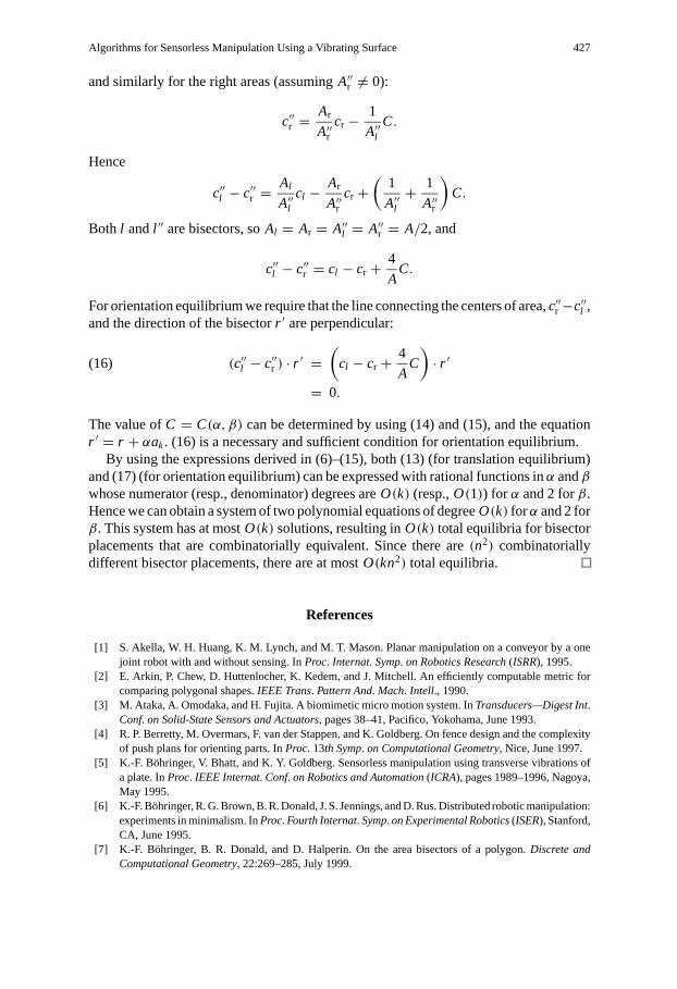
Algorithms for Sensorless Manipulation Using a Vibrating Surface 427
and similarly for the right areas (assumingA′′r 6= 0):
c′′r =Ar
A′′rcr − 1
A′′lC.
Hence
c′′l − c′′r =Al
A′′lcl − Ar
A′′rcr +
(1
A′′l+ 1
A′′r
)C.
Both l andl ′′ are bisectors, soAl = Ar = A′′l = A′′r = A/2, and
c′′l − c′′r = cl − cr + 4
AC.
For orientation equilibrium we require that the line connecting the centers of area,c′′r −c′′l ,and the direction of the bisectorr ′ are perpendicular:
(c′′l − c′′r ) · r ′ =(
cl − cr + 4
AC
)· r ′(16)
= 0.
The value ofC = C(α, β) can be determined by using (14) and (15), and the equationr ′ = r + αak. (16) is a necessary and sufficient condition for orientation equilibrium.
By using the expressions derived in (6)–(15), both (13) (for translation equilibrium)and (17) (for orientation equilibrium) can be expressed with rational functions inα andβwhose numerator (resp., denominator) degrees areO(k) (resp.,O(1)) for α and 2 forβ.Hence we can obtain a system of two polynomial equations of degreeO(k) forα and 2 forβ. This system has at mostO(k) solutions, resulting inO(k) total equilibria for bisectorplacements that are combinatorially equivalent. Since there are(n2) combinatoriallydifferent bisector placements, there are at mostO(kn2) total equilibria.
References
[1] S. Akella, W. H. Huang, K. M. Lynch, and M. T. Mason. Planar manipulation on a conveyor by a onejoint robot with and without sensing. InProc. Internat. Symp. on Robotics Research(ISRR), 1995.
[2] E. Arkin, P. Chew, D. Huttenlocher, K. Kedem, and J. Mitchell. An efficiently computable metric forcomparing polygonal shapes.IEEE Trans. Pattern And. Mach. Intell., 1990.
[3] M. Ataka, A. Omodaka, and H. Fujita. A biomimetic micro motion system. InTransducers—Digest Int.Conf. on Solid-State Sensors and Actuators, pages 38–41, Pacifico, Yokohama, June 1993.
[4] R. P. Berretty, M. Overmars, F. van der Stappen, and K. Goldberg. On fence design and the complexityof push plans for orienting parts. InProc. 13th Symp. on Computational Geometry, Nice, June 1997.
[5] K.-F. Bohringer, V. Bhatt, and K. Y. Goldberg. Sensorless manipulation using transverse vibrations ofa plate. InProc. IEEE Internat. Conf. on Robotics and Automation(ICRA), pages 1989–1996, Nagoya,May 1995.
[6] K.-F. Bohringer, R. G. Brown, B. R. Donald, J. S. Jennings, and D. Rus. Distributed robotic manipulation:experiments in minimalism. InProc. Fourth Internat. Symp. on Experimental Robotics(ISER), Stanford,CA, June 1995.
[7] K.-F. Bohringer, B. R. Donald, and D. Halperin. On the area bisectors of a polygon.Discrete andComputational Geometry, 22:269–285, July 1999.
428 K.-F. Bohringer, V. Bhatt, B. R. Donald, and K. Goldberg
[8] K.-F. Bohringer, B. R. Donald, and N. C. MacDonald. Upper and lower bounds for programmable vectorfields with applications to MEMS and vibratory plate parts feeders. In J.-P. Laumond and M. Overmars,editors,Algorithms for Robotic Motion and Manipulation, pages 255–276. A. K. Peters, Ltd, Wellesley,MA 02181, 1997.
[9] K.-F. Bohringer, B. R. Donald, N. C. MacDonald, G. T. A. Kovacs, and J. W. Suh. Computational methodsfor design and control of MEMS micromanipulator arrays.IEEE Computer Science and Engineering,pages 17–29, January–March 1997.
[10] K.-F. Bohringer, B. R. Donald, R. Mihailovich, and N. C. MacDonald. Sensorless manipulation usingmassively parallel microfabricated actuator arrays. InProc. IEEE Internat. Conf. on Robotics andAutomation(ICRA), pages 826–833, San Diego, CA, May 1994.
[11] K.-F. Bohringer, B. R. Donald, R. Mihailovich, and N. C. MacDonald. A theory of manipulation andcontrol for microfabricated actuator arrays. InProc. IEEE Workshop on Micro Electro MechanicalSystems(MEMS), pages 102–107, Oiso, January 1994.
[12] K.-F. Bohringer, K. Goldberg, M. B. Cohn, R. Howe, and A. Pisano. Parallel microassembly withelectrostatic force fields. InProc. IEEE Int.Conf.on Robotics and Automation(ICRA), Leuven, Belgium,May 1998.
[13] G. Boothroyd, C. Poli, and L. E. Murch.Automatic Assembly. Marcel Dekker, New York, 1982.[14] R. Brooks. A layered intelligent control system for a mobile robot.IEEE J. Robotics Automat., (2),
1986.[15] M. E. Caine. The Design of Shape from Motion Constraints. Ph.D. thesis, Department of Computer
Science, Massachusetts Institute of Technology, Cambridge, MA, 1993.[16] J. Canny and K. Goldberg. “RISC” for industrial robotics: recent results and open problems. InProc.
IEEE Internat. Conf. on Robotics and Automation(ICRA), May 1994.[17] Y. Chitour, A. Marigo, D. Prattichizzo, and A. Bicchi. Rolling polyhedra on a plane, analysis of the
reachable set. InProc. Internat. Workshop on Algorithmic Foundations of Robotics(WAFR), Toulouse,July 1996.
[18] E. F. Chladni.Entdeckungenuber die Theorie des Klanges. Weidmanns Erben und Reich, Leipzig, 1787.[19] M. Coutinho and P. Will. The intelligent motion surface: a hardware/software tool for the assembly of
meso-scale devices. InProc. IEEE Internat. Conf. on Robotics and Automation(ICRA), Albuquerque,NM, April 1997.
[20] M. Dıaz and J. O’Rourke. Ham-sandwich sectioning of polygons. InProc. 2nd Canadian Conf. onComputational Geometry, pages 98–101, Ottawa, 1990.
[21] B. R. Donald. The complexity of planar compliant motion planning with uncertainty.Algorithmica,5(3):353–382, 1990.
[22] B. R. Donald, J. Jennings, and D. Rus. Information invariants for distributed manipulation. In K. Gold-berg, D. Halperin, J.-C. Latombe, and R. Wilson, editors,Proc. Algorithmic Foundations of Robotics(WAFR), pages 431–459, Wellesley, MA, 1995. A. K. Peters, Boston, MA.
[23] B. R. Donald and P. Xavier. Provably good approximation algorithms for optimal kinodynamic planningfor cartesian robots and open chain manipulators.Algorithmica, 14(6):480–530, November 1995.
[24] M. A. Erdmann. An Exploration of Nonprehensile Two-Palm Manipulation: Planning and Execution.Technical report, Carnegie Mellon University, Pittsburgh, PA, 1996.
[25] M. A. Erdmann and M. T. Mason. An exploration of sensorless manipulation.IEEE J.Robotics Automat.,4(4), August 1988.
[26] M. A. Erdmann and M. T. Mason. Nonprehensile manipulation. InProc. Robotic Motion and Manipu-lation, Toulouse, July 1996.
[27] G. T. Farnum and B. Davis. Delivering the part.Manufacturing Engrg, March 1986.[28] K. Y. Goldberg. Orienting polygonal parts without sensing.Algorithmica, 10(2/3/4):201–225,
August/September/October 1993.[29] D. D. Grossman and M. W. Blasgen. Orienting mechanical parts by computer-controlled manipulator.
IEEE Trans. Systems Man Cybernet., 5, 1975.[30] J. Hartley. Picking parts from a bowlfeeder with image sensing.Sensor Rev., 1(1), January 1981.[31] J. W. Hill. Programmable bowl feeder design based on computer vision.Assembly Automat., 1(1),
November 1980.[32] H. Hitakawa. Advanced parts orientation system has wide application.Assembly Automat., 8(3),
1988.

Algorithms for Sensorless Manipulation Using a Vibrating Surface 429
[33] L. Kavraki. Part orientation with programmable vector fields: two stable equilibria for most parts. InProc. IEEE Internat. Conf. on Robotics and Automation(ICRA), Albuquerque, NM, April 1997.
[34] S. Konishi and H. Fujita. System design for cooperative control of arrayed microactuators. InProc.IEEE Workshop on Micro Electro Mechanical Systems(MEMS), pages 324–329, Amsterdam, January1995.
[35] W. Liu and P. Will. Parts manipulation on an intelligent motion surface. InInternat. Conf. on IntelligentRobots and Systems. IEEE/RSJ, 1995.
[36] W. Liu and P. Will. Parts manipulation on an intelligent motion surface. InIEEE/RSJ Internat. Workshopon Intelligent Robots & Systems(IROS), volume 3, pages 399–404, Pittsburgh, PA, Aug. 1995.
[37] T. Lozano-P´erez, M. Mason, and R. Taylor. Automatic synthesis of fine-motion strategies for robots.Internat. J. Robotics Res., 3(1), 1984.
[38] J. E. Luntz and W. Messner. A distributed control system for flexible materials handling.IEEE Trans.Control Systems, 17(1), February 1997.
[39] J. E. Luntz, W. Messner, and H. Choset. Parcel manipulation and dynamics with a distributed actuatorarray: the virtual vehicle. InProc. IEEE Internat. Conf. on Robotics and Automation(ICRA), pages1541–1546, Albuquerque, NM, April 1997.
[40] T. McGeer. Passive dynamic walking.Internat. J. Robotics Res., 1990.[41] B. Mirtich and J. Canny. Impulse-based simulation of rigid bodies. InProc. Symp. on Interactive3D
Graphics, Monterrey, CA, 1995.[42] P. Moncevicz, M. Jakiela, and K. Ulrich. Orientation and insertion of randomly presented parts using
viratory agitation. InProc. ASME3rd Conf. on Flexible Assembly Systems, September 1991.[43] J. L. Nevins and D. E. Whitney. Computer-controlled assembly.Scientific American, 1978.[44] D. Pherson. Programmable feeder for non-rotational parts. InProc. 15th CIRP Internat. Seminar on
Manufacturing Systems, 1983.[45] W. Press, B. Flannery, S. Tenkolsky, and W. Vetterling.Numerical Recipes in C. Cambridge University
Press, New York, 1988.[46] M. H. Raibert, J. K. Hodgins, R. R. Playter, and R. P. Ringrose. Animation of legged maneuvers: jumps,
somersaults, and gait transitions.J. Robotics Soc. Japan, 11(3):333–341, 1993.[47] A. Rao and K. Goldberg. Shape from diameter: recognizing polygonal parts with a parallel-jaw gripper.
Internat. J. Robotics Res., 13(1), February 1994.[48] J. W. S. Rayleigh.The Theory of Sound, 2nd edition. Dover, New York, 1945.[49] A. H. Redford and E. Lo.Robots in Assembly. Halsted Press, New York, 1986.[50] D. Reznik, S. Brown, and J. F. Canny. Dynamic simulation as a design tool for a microactuator array.
In Proc. IEEE Internat. Conf. on Robotics and Automation(ICRA), Albuquerque, NM, April 1997.[51] D. Reznik, J. F. Canny, and K. Y. Goldberg. Analysis of part motion on a longitudinally vibrating plate.
In Proc. IEEE/RSJ Internat. Workshop on Intelligent Robots & Systems(IROS), Grenoble, September1997.
[52] F. J. Riley.Assembly Automation, A Management Handbook. Industrial Press, New York, 1983.[53] B.-Z. Sandler.Robotics: Designing the Mechanisms for Automated Machinery. Prentice-Hall, Engle-
wood Cliffs, NJ, 1991.[54] B. J. Schroer. Electronic parts presentation using vibratory bowl feeders.Robotics, 3, 1987.[55] N. C. Singer and W. P. Seering. Utilizing dynamic stability to orient parts.J. Appl. Mech., 54:961–966,
December 1987.[56] T. Suzuki. An approach to a flexible part-feeding system. InProc. 1st Internat. Conf. on Assembly
Automation, 1980.[57] P. Swanson, R. Burridge, and D. Koditschek. Global asymptotic stability of a passive juggler: a parts
feeding strategy. InProc. IEEE Internat. Conf. on Robotics and Automation(ICRA), Nagoya, May 1995.[58] S. Timoshenko.Theory of Plates and Shells. McGraw-Hill, New York, 1940.[59] N. D. Tran and K. W. Chan. Object behavior using a vibrating plate testbed for part presentation research.
Term Paper 304-494, Electrical Engineering Department, McGill University, December 1995. InstructorVince Hayward.
[60] N. B. Zumel and M. A. Erdmann. Nonprehensile two palm manipulation with non-equilibrium transitionsbetween stable states. InProc. IEEE Internat. Conf. on Robotics and Automation(ICRA), Minneapolis,MN, April 1996.