Embed Size (px)
Citation preview

Lecture Noteson
Laplace and z-transforms
Ali Sinan [email protected]
http://www.fen.bilkent.edu.tr/˜sertoz
11 April 2003
1 Introduction
These notes are intended to guide the student through problem solving usingLaplace and z-transform techniques and is intended to be part of MATH 206course. These notes are freely composed from the sources given in the bibli-ography and are being constantly improved. Check the date above to see ifthis is a new version.
You are welcome to contact me through e-mail if you have any comments onthese notes such as praise, criticism or suggestions for further improvements.
1

MATH 206 Complex Calculus and Transform Techniques [11 April 2003] 2
2 Laplace Transformation
The main application of Laplace transformation for us will be solving somedifferential equations. A differential equation will be transformed by Laplacetransformation into an algebraic equation which will be solvable, and thatsolution will be transformed back to give the actual solution of the DE westarted with.
We define the Laplace Transform of a function f : [0,∞) → C as
L(f(t)) =
∫ ∞
0
e−stf(t)dt for s ∈ C
We sometimes use F (s) to denote L(f(t)) if there is no confusion. But bewareof conflicting notation in the literature.
Euler1 was the first one to use this transformation to solve certain differentialequations in 1737. Later Laplace2 independently used it in his book TheorieAnalytique de Probabilites in 1812, [6, p285].
2.1 Existence of Laplace Transformation
It is clear that L(f) does not exist for every function f . For example it
can be easily verified that L(et2) does not exist, i.e. the associated integralclearly diverges. However L exists for a large class of functions. For exampleconsider the following class of functions:
A function f : [0,∞) → C is said to be of exponential order a if there arepositive real constants M , T and a such that |f(t)| ≤ Meat for all t ≥ T .
L(f) exists if f is integrable on [0, b] for every b > 0 and f is of exponentialorder a for some a > 0. In this case F (s) is defined if and only if Re s > a.Moreover observe from the definition that lim
Re s→∞F (s) = 0.
A word of relief: We will basically be using Laplace transform techniques to
1Leonhard Euler 1707-1783.2Pierre-Simon Laplace 1749-1827.

MATH 206 Complex Calculus and Transform Techniques [11 April 2003] 3
solve differential equations. Most differential equations with initial values willhave a unique solution, see for example [7, p498-Thm 10.6 and p501-Thm10.8]. We therefore formally apply Laplace transform techniques, withoutchecking for validity, and if in the end the function we find solves the differ-ential equation then it is the solution. For this reasons most tables of Laplacetransforms do not give the range of validity and are therefore wrong per sebut perfectly acceptable given the overall purpose.
2.2 Elementary Properties of Laplace Transformation
Before we start calculating the Laplace transformation of any function wecan derive some results which reflect our expectations from L(f) using onlythe elementary properties of integrals.
Suppose α, β ∈ C and f, g functions for which Laplace transformation exists.Then:
• L(αf(t) + βg(t)) = αF (s) + βG(s). (Linearity)
• L(eαtf(t)) = F (s− α). (Shift property)
• Suppose f and all its derivatives up to and including order n are con-tinuous on [0,∞) with f and each derivative having Laplace transfor-mation. Then
L(f (n)(t)) = snF (s)− sn−1f(0)− · · · − sn−k−1f (k)(0)− · · · − f (n−1)(0).
In particular
L(f ′(t)) = sF (s)− f(0),
L(f ′′(t)) = s2F (s)− sf(0)− f ′(0).
• If f is continuous on (0,∞), then L
(∫ t
0
f(u)du
)= F (s)/s.
• If f is continuous on (0,∞), then L(tnf(t)) = (−1)nF (n)(s).

MATH 206 Complex Calculus and Transform Techniques [11 April 2003] 4
2.3 Transforms of some elementary functions
Before we apply Laplace transformation techniques to differential equationswe need to actually see the transformation of some functions. We generallyneed some tables listing the Laplace transforms of some elementary functions.Then using the properties listed in the previous section we can find theLaplace transformation of most functions.
We begin by a table where each entry can be found by direct integration,using the definition of the Laplace transformation.
In the following list, α and β are complex constants and n is a nonnegativeinteger.
• L(α) =α
s.
• L(t) =1
s2.
In general L(tn) =n!
sn+1.
• L(eαt) =1
s− α, where Re s > Re α.
• L(sin αt) =α
s2 + α2, where Re s > −Im α.
• L(cos αt) =s
s2 + α2, where Re s > −Im α.
• L(sinh αt) =α
s2 − α2.
• L(cosh αt) =s
s2 − α2.
The next three formulas follow from the general property L(tnf(t)) = (−1)nF (n)(s).
• L(t sin αt) =2αs
(s2 + α2)2.

MATH 206 Complex Calculus and Transform Techniques [11 April 2003] 5
• L(t cos αt) =s2 − α2
(s2 + α2)2.
• L(te−αt) =1
(s + α)2, where α > 0.
In general L(tne−αt) =n!
(s + α)n+1, where α > 0.
The next formulas follow from the shift property L(eαtf(t)) = F (s− α).
• L(e−αt sin βt) =β
(s + α)2 + β2, where α > 0.
• L(e−αt sinh βt) =β
(s + α)2 − β2, where α > 0.
• L(e−αt cos βt) =s + α
(s + α)2 + β2, where α > 0.
• L(e−αt cosh βt) =s + α
(s + α)2 − β2, where α > 0.
2.4 Inverse Laplace Transformation
If L(f(t)) = F (s), then f(t) is called the inverse Laplace transform of F (s)and is denoted by L−1(F (s)) = f(t).
If we assume that the functions whose Laplace transforms exist are going tobe taken as continuous then no two different functions can have the sameLaplace transform. Functions that differ only at isolated points can have thesame Laplace transform. Such uniqueness theorems allow us to find inverseLaplace transform by looking at Laplace transform tables.
Example:-2.1 Find the function f(t) for which L(f(t)) =2s + 3
s2 + 4s + 13.
Solution: By completing the denominator to a square and playing withthe numerator we write L(f(t)) as
2s + 3
s2 + 4s + 13=
2(s + 2)
(s + 2)2 + 9− 1
(s + 2)2 + 9.

MATH 206 Complex Calculus and Transform Techniques [11 April 2003] 6
Here we try to recognize each part on the right as Laplace transform ofsome function, using a table of Laplace transforms. For example we notethat L(e−2t cos(3t)) = s+2
(s+2)2+9and L(e−2t sin(3t)) = 3
(s+2)2+9. Using this
information together with the fact that Laplace transform is a linear operatorwe find that
L−1
{2s + 3
s2 + 4s + 13
}= L−1
{2(s + 2)
(s + 2)2 + 9
}− L−1
{1
(s + 2)2 + 9
}
= 2e−2t cos(3t)− 1
3e−2t sin(3t)
= f(t).
Note: Inverse Laplace of a function can also be found using integrals andresidues. This is given in your textbook [3, sections 66-67].
2.5 Convolution
When f(t) and g(t) are defined for t > 0, and are piecewise continuous, thentheir convolution, denoted by f ∗ g, is defined as
(f ∗ g)(t) =
∫ t
0
f(t− u)g(u)du, for 0 ≤ t < ∞.
Convolution has some immediate properties following from the above defini-tion:1. f ∗ g = g ∗ f .2. f ∗ (cg) = (cf) ∗ g = c(f ∗ g), where c is a constant.3. f ∗ (g + h) = f ∗ g + f ∗ h.4. f ∗ (g ∗ h) = (f ∗ g) ∗ h.
In particular the following property is useful:
L−1 {F (s)G(s)} = f ∗ g where L(f) = F and L(g) = G.
In other words;L((f ∗ g)(t)) = F (s)G(s).

MATH 206 Complex Calculus and Transform Techniques [11 April 2003] 7
Example:-2.2 An equation of the form
x(t) = f(t) +
∫ t
0
h(t− u)x(u)du
where f and h are known functions and x is the unknown function is calledVolterra3 integral equation. Note that the given integral is a convolutionintegral. Letting capital letters denote the Laplace transform of the corre-sponding function we apply Laplace operator to each side of the Volterraequation to obtain
X(s) = F (s) + H(s)X(s).
Solving for X(s) we get
X(s) =F (s)
1−H(s),
which can theoretically be inverted by Laplace transformation to give therequired x(t).
Example:-2.3 Solve the Volterra equation
x(t) = e−t − 4
∫ t
0
cos 2(t− u)x(u)du.
Solution: Applying Laplace operator to each side we get
X(s) =1
s + 1− 4X(s)
s
s2 + 4.
Solving for X(s) we get
X(s) =s2 + 4
(s + 1)(s + 2)2
=5
s + 1− 4
s + 2+
8
(s + 2)2.
Applying Laplace inverse transformation to both sides of this equation wefinally get
x(s) = 5e−t − 4e−2t − 8te−2t.
3Vito Volterra 1860-1940.

MATH 206 Complex Calculus and Transform Techniques [11 April 2003] 8
2.6 Heaviside unit function
The Heaviside unit function is denoted and definedas
H(t) =
{0, if t < 0;1, if t ≥ 0.
0
1
t
By directly integrating the Heaviside4 function we find that
L(H(t− a)) =e−sa
sfor a > 0.
In particular
L(H(t)) =1
s.
Compare this to the case where we apply Laplace operator to f(t) = 1 fort > 0.
Again by direct integration we find the important shift property
L(H(t− a)f(t− a)) = e−asL(f(t)), for a > 0.
Example:-2.4
L(H(t− 2) cos(t− 2)) =se−2s
s2 + 1.
Example:-2.5
L(H(t− 2) sin(t− 2)) =e−2s
s2 + 1.
Example:-2.6
L(H(t− 2) cos(t)) = L(H(t− 2) cos ((t− 2) + 2))
= L(H(t− 2) (cos(t− 2) cos(2)− sin(t− 2) sin(2)))
= cos(2)L(H(t− 2) cos(t− 2))− sin(2)L(H(t− 2) sin(t− 2))
=
(s cos(2)
(s2 + 1)− sin(2)
(s2 + 1)
)e−2s.
4Oliver Heaviside 1850-1925.
MATH 206 Complex Calculus and Transform Techniques [11 April 2003] 9
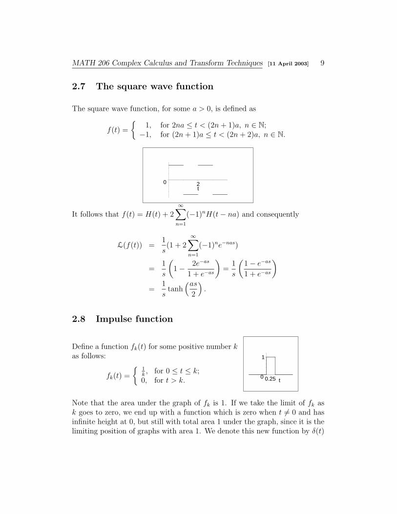
2.7 The square wave function
The square wave function, for some a > 0, is defined as
f(t) =
{1, for 2na ≤ t < (2n + 1)a, n ∈ N;
−1, for (2n + 1)a ≤ t < (2n + 2)a, n ∈ N.
0 2t
It follows that f(t) = H(t) + 2∞∑
n=1
(−1)nH(t− na) and consequently
L(f(t)) =1
s(1 + 2
∞∑n=1
(−1)ne−nas)
=1
s
(1− 2e−as
1 + e−as
)=
1
s
(1− e−as
1 + e−as
)
=1
stanh
(as
2
).
2.8 Impulse function
Define a function fk(t) for some positive number kas follows:
fk(t) =
{1k, for 0 ≤ t ≤ k;
0, for t > k.0
1
0.25 t
Note that the area under the graph of fk is 1. If we take the limit of fk ask goes to zero, we end up with a function which is zero when t 6= 0 and hasinfinite height at 0, but still with total area 1 under the graph, since it is thelimiting position of graphs with area 1. We denote this new function by δ(t)

MATH 206 Complex Calculus and Transform Techniques [11 April 2003] 10
and call it the impulse function or Dirac5 delta function.
To find the Laplace transform of the impulse function we start with theLaplace of fk:
L(fk(t)) =
∫ ∞
0
fk(t)e−stdt
=
∫ k
0
1
ke−stdt =
[−e−st
sk
]k
0
= − 1
sk(e−sk − 1) = 1− sk
2!+
(sk)2
3!+ · · · .
Taking the limit as k → 0 we find
L(δ(t)) = 1.
An impulse of size a is represented by aδ(t) and an impulse which is delayedby time T is denoted by δ(t− T ). Recalling the shift property, i.e. L(H(t−T )f(t−T )) = e−sT L(f(t)), we can immediately write the Laplace of a delayedimpulse function of a certain size:
L(aδ(t− T )) = aL(H(t− T )δ(t− T )) = ae−sT .
Example:-2.7 Solve the initial value problem
x′′(t) + 3x′(t) + 2x(t) = 5δ(t− 2)
where x(0) = 4 and x′(0) = 0.
Solution: Transforming by Laplace we get(s2 + 3s + 2)X(s)− 4s− 12 = 5e−2s. Solving for X(s) we find
X(s) =5e−2s + 4s + 12
(s + 1)(s + 2).
Here we observe that
1
(s + 1)(s + 2)=
1
s + 1− 1
s + 2,
s
(s + 1)(s + 2)=
−1
s + 1+
2
s + 2
5Paul Adrien Maurice Dirac 1902-1984.

MATH 206 Complex Calculus and Transform Techniques [11 April 2003] 11
and recall the formulas
L(e−at) =1
s + a, and
L(H(t− k)f(t− k)) = e−ksL(f(t)).
Applying inverse Laplace transformation with these formulas in mind we get
x(t) = 5(e−(t−2) − e−2(t−2))H(t− 2) + 4(2e−2t − e−t) + 12(e−t − e−2t)
= 5(e−(t−2) − e−2(t−2))H(t− 2)− 4e−2t + 8e−t.
2.9 Unsorted solved problems
Problem:-1 Find L(g(t)), where
g(t) =
{0 for 0 < t < 1
3t for 1 ≤ t0
5
1.5t
Solution: First recall that L(H(t− a)f(t− a)) = e−asF (s). We thereforewrite 3t in shifted form: 3t = 3(t−1)+3. Let f(t) = 3t+3. Then f(t−1) = 3tand H(t− 1)f(t− 1) = g(t), for t > 0. Hence
L(g(t)) = L(H(t− 1)f(t− 1)) = e−sL(f(t))
= e−sL(3t + 3)
= e−s
(3
s2+
3
s
).
Problem:-2 Find L(g(t)), where
g(t) =
{0 for 0 < t < π
cos t for π ≤ t
0 3.5t

MATH 206 Complex Calculus and Transform Techniques [11 April 2003] 12
Solution: Observe that cos t = − cos(t − π). Setting f(t) = − cos t, wenote that g(t) = H(t− π)f(t− π). So
L(g(t)) = L(H(t− π)f(t− π)
= e−πsL(f(t))
= e−πs −s
s2 + 1.
Problem:-3 Find the inverse Laplace transform of F (s) =1
s3 − s2 + s− 1.
Solution:
F (s) =1
(s− 1)(s2 + 1)
=1
2
(1
s− 1− s
s2 + 1− 1
s2 + 1
).
Hence
L−1(F (s)) =1
2
(L−1(
1
s− 1)− L−1(
s
s2 + 1)− L−1(
1
s2 + 1)
)
=1
2
(et − cos t− sin t
).
Problem:-4 Find the inverse Laplace transform of F (s) =2
s+
e−3s
s2.
Solution:
L−1(F (s)) = L−1(2
s) + L−1(
e−3s
s2)
= 2 + H(t− 3)(t− 3).
Problem:-5 Solve f ′′(t) + f(t) = t, where f(0) = 1, f ′(0) = −2.Solution:
L(f ′′(t)) + L(f(t)) = L(t)(s2F (s)− sf(0)− f ′(0)
)+ F (s) =
1
s2

MATH 206 Complex Calculus and Transform Techniques [11 April 2003] 13
s2F (s)− s + 2 + F (s) =1
s2.
Solving for F (s);
F (s) =1
s2+
s
s2 + 1− 3
s2 + 1,
and applying inverse Laplace transform
L−1
(1
s2+
s
s2 + 1− 3
s2 + 1
)= t + cos t− 3 sin t = f(t).
Problem:-6 Solve the initial value problem y′′(t) + y(t) = f(t), y(0) =y′(0) = 0, where f(t) = n + 1 for nπ ≤ t < (n + 1)π, n ∈ N, i.e.f(t) =
∑∞k=0 H(t− kπ).
Solution: We plan to take the Laplace transform of both sides of thedifferential equation. For this observe that
L(y′′(t)) = s2Y (s)− sy(0)− y′(0) = s2Y (s)
L(y(t)) = Y (s)
L(f(t)) = L
( ∞∑
k=0
H(t− kπ)
)
=∞∑
k=0
L(H(t− kπ)) =∞∑
k=0
e−kπs
s.
Putting these together, the differential equation becomes
s2Y (s) + Y (s) =1
s
∞∑
k=0
e−kπs
and solving for Y (s)
Y (s) =
(1
s(s2 + 1)
) ∞∑
k=0
e−kπs
=1
s
∞∑
k=0
e−kπs − s
s2 + 1
∞∑
k=0
e−kπs.
Before applying the inverse Laplace transform to both sides recall thatL(H(t− a) cos(t− a)) = ( s
s2+1)e−as.

MATH 206 Complex Calculus and Transform Techniques [11 April 2003] 14
Define a new function
g(t) =∞∑
k=0
H(t− kπ) cos(t− kπ).
We can finally apply the inverse Laplace transform to Y (s) to find
L−1(Y (s)) = L−1(1
s
∞∑
k=0
e−kπs)− L−1(s
s2 + 1
∞∑
k=0
e−kπs)
y(t) = f(t)− g(t).
Problem:-7 Solve the initial value problem y′′(t)+y(t) = 3 sin 2t, t ∈ [0,∞],y(0) = 1, y′(0) = −2.
Solution: Letting Y (s) = L(y(t)), note that
L(y′′(t)) = s2Y (s)− sy(0)− y′(0)
= s2Y (s)− s + 2,
L(sin 2t) =2
s2 + 4.
Taking the inverse Laplace of both sides of the differential equation we get
s2Y (s)− s + 2 + Y (s) =6
s2 + 4.
Solving for Y (s) we get
Y (s) =s
s2 + 1− 2
s2 + 4.
Taking the inverse Laplace transform gives
y(t) = cos t− sin 2t.

MATH 206 Complex Calculus and Transform Techniques [11 April 2003] 15
Problem:-8 Define a function f(t) as
f(t) =
0 if t < 11 if 1 ≤ t < 22 if 2 ≤ t < 31 if 3 ≤ t < 40 if 4 ≤ t
0
2
5t
Note that f(t) = H(t− 1) + H(t− 2)−H(t− 3)−H(t− 4).Solve the initial value problem y′′ − 3y′ + 2y = f(t), y(0) = y′(0) = 0.
Solution: Taking the Laplace transform of both sides gives
s2Y − 3sY + 2Y =1
s(e−s + e−2s − e−3s − e−4s).
Set A = (e−s + e−2s − e−3s − e−4s). Then solving for Y gives
Y =A
s(s− 1)(s− 2)
=1
2
A
s− A
s− 1+
1
2
A
s− 2.
Recall that
L(H(t− a)eb(t−a)) =eas
s− b.
Taking the inverse Laplace transform of Y gives
y(t) =2∑
k=1
(1
2− et−k +
1
2e2(t−k)
)H(t− k)
−4∑
k=3
(1
2− et−k +
1
2e2(t−k)
)H(t− k)

MATH 206 Complex Calculus and Transform Techniques [11 April 2003] 16
Problem:-9 Find the solution of the system
dx
dt− 6x + 3y = 8et
dy
dt− 2x− y = 4et
with initial conditions x(0) = −1, y(0) = 0.
Solution: Taking the Laplace transform of the system and simplifying wefind
(s− 6)X + 3Y =−s + 9
s− 1
−2X + (s− 1)Y =4
s− 1
Solving for X and Y we find
X =−s + 7
(s− 1)(s− 4)=
−2
s− 1+
1
s− 4
Y =2
(s− 1)(s− 4)=−2/3
s− 1+
2/3
s− 4.
Applying inverse Laplace transform to these equations gives
x(t) = −2et + e4t
y(t) = −2
3et +
2
3e4t.

MATH 206 Complex Calculus and Transform Techniques [11 April 2003] 17
Problem:-10 Find that solution ofux(x, t) = 2ut(x, t) + u(x, t), u(x, 0) = 6e−3x, which is bounded for x > 0,t > 0.Solution: First note that
L(ux(x, t)) =
∫ ∞
0
e−st ∂u(x, t)
∂xdt
=d
dx
∫ ∞
0
e−stu(x, t)dt
=d
dxU(x, s).
It follows from general properties of Laplace transform that
L(ut(x, t)) = sU(x, s)− u(x, 0).
Putting these together, the given PDE transforms to
d
dxU − (2s + 1)U = −12e−3x.
Multiplying both sides by the integration factor e−(2s+1)x gives
d
dx(Ue−(2s+1)x) = −12e−(2s+4)x.
Integrating this gives
Ue−(2s+1)x =6
s + 2e−(2s+4)x + c,
or
U =6
s + 2e−3x + ce(2s+1)x.
Since u(x, t) must stay bounded as x → ∞, likewise U(x, s) must staybounded when x →∞. So we must choose c = 0, and then we have
U(x, s) =6
s + 2e−3x,
and hence
u(x, t) = 6e−2t−3x.
MATH 206 Complex Calculus and Transform Techniques [11 April 2003] 18
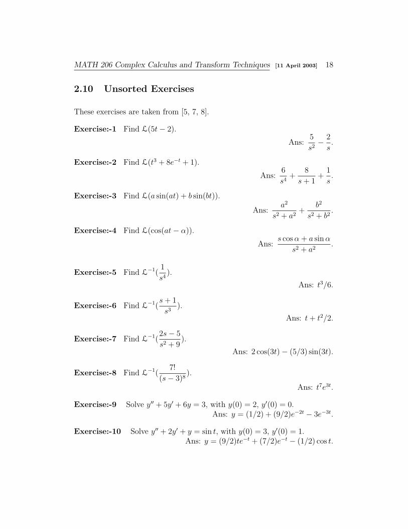
2.10 Unsorted Exercises
These exercises are taken from [5, 7, 8].
Exercise:-1 Find L(5t− 2).
Ans:5
s2− 2
s.
Exercise:-2 Find L(t3 + 8e−t + 1).
Ans:6
s4+
8
s + 1+
1
s.
Exercise:-3 Find L(a sin(at) + b sin(bt)).
Ans:a2
s2 + a2+
b2
s2 + b2.
Exercise:-4 Find L(cos(at− α)).
Ans:s cos α + a sin α
s2 + a2.
Exercise:-5 Find L−1(1
s4).
Ans: t3/6.
Exercise:-6 Find L−1(s + 1
s3).
Ans: t + t2/2.
Exercise:-7 Find L−1(2s− 5
s2 + 9).
Ans: 2 cos(3t)− (5/3) sin(3t).
Exercise:-8 Find L−1(7!
(s− 3)8).
Ans: t7e3t.
Exercise:-9 Solve y′′ + 5y′ + 6y = 3, with y(0) = 2, y′(0) = 0.Ans: y = (1/2) + (9/2)e−2t − 3e−3t.
Exercise:-10 Solve y′′ + 2y′ + y = sin t, with y(0) = 3, y′(0) = 1.Ans: y = (9/2)te−t + (7/2)e−t − (1/2) cos t.

MATH 206 Complex Calculus and Transform Techniques [11 April 2003] 19
Exercise:-11 ([5, p50]) Solve the differential equationd2x
dt2+ 3
dx
dt+ 2x = 5δ(t− 2), with x(0) = 4, x′(0) = 0.
Ans: 5(e−(t−2) − e−2(t−2))H(t− 2) + 8e−t − 4e−2t.
Exercise:-12 [7, p456] Solve the following linear system using Laplacetransform technique:
dx
dt+ y = 3e2t
dy
dt+ x = 0
x(0) = 2 y(0) = 0.
Ans: x = −et
2+
e−t
2+ 2e2t, y =
et
2+
e−t
2− e2t.
Exercise:-13 [7, p457] Solve the following linear system using Laplacetransform technique:
2dx
dt+
dy
dt− x− y = e−t
dx
dt+
dy
dt+ 2x + y = et
x(0) = 2 y(0) = 1.
Ans: x = 8 sin t + 2 cos t, y = −13 sin t + cos t +et
2− e−t
2.

MATH 206 Complex Calculus and Transform Techniques [11 April 2003] 20
Exercise:-14 [7, p457] Solve the following linear system using Laplacetransform technique:
d2x
dt2− 3
dx
dt+
dy
dt+ 2x− y = 0
dx
dt+
dy
dt− 2x + y = 0
x(0) = 0 x′(0) = 0 y(0) = −1.
Ans: x = −1 + 2et − e2t, y = −2 + et.
Exercise:-15 [8, p484] Solve the following differential equation usingLaplace transform technique:
f ′′(t)− f ′(t)− 2f(t) = e−t sin 2t, with f(0) = 0 and f ′(0) = 2.
Ans: f(t) =28
39e2t − 5
6e−t − 1
13e−t sin 2t +
3
26e−t cos 2t.
MATH 206 Complex Calculus and Transform Techniques [11 April 2003] 21
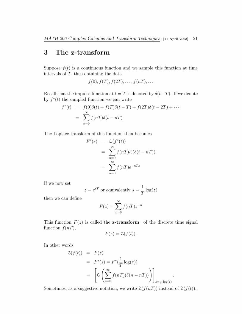
3 The z-transform
Suppose f(t) is a continuous function and we sample this function at timeintervals of T , thus obtaining the data
f(0), f(T ), f(2T ), . . . , f(nT ), . . .
Recall that the impulse function at t = T is denoted by δ(t−T ). If we denoteby f ∗(t) the sampled function we can write
f ∗(t) = f(0)δ(t) + f(T )δ(t− T ) + f(2T )δ(t− 2T ) + · · ·
=∞∑
n=0
f(nT )δ(t− nT )
The Laplace transform of this function then becomes
F ∗(s) = L(f ∗(t))
=∞∑
n=0
f(nT )L(δ(t− nT ))
=∞∑
n=0
f(nT )e−nTs
If we now set
z = esT or equivalently s =1
Tlog(z)
then we can define
F (z) =∞∑
n=0
f(nT )z−n
This function F (z) is called the z-transform of the discrete time signalfunction f(nT ),
F (z) = Z(f(t)).
In other words
Z(f(t)) = F (z)
= F ∗(s) = F ∗(1
Tlog(z))
=
[L
( ∞∑n=0
f(nT )(δ(n− nT ))
)]
s= 1T
log(z)
.
Sometimes, as a suggestive notation, we write Z(f(nT )) instead of Z(f(t)).

MATH 206 Complex Calculus and Transform Techniques [11 April 2003] 22
Example:-3.8 Find Z(H(nT )). Here we are sampling the function f(t) =H(t), the unit step function, or the Heaviside function, and obtaining thesample f(n) = 1 for all n ≥ 0.
Solution:
F (z) =∞∑
n=0
1 z−n = 1 + z−1 + z−2 + · · ·
=1
1− z−1=
z
z − 1.
Hence we find that
Z(H(nT )) =z
z − 1for |z| > 1.
Example:-3.9 Find the z-transform of the sampled function f(nT ) for f(t) =t, (the ramp function).
Solution: We find that f(nT ) = nT . Hence
F (z) = Tz−1 + 2Tz−2 + 3Tz−3 + · · ·=
T
z(1− z−1)2
=Tz
(z − 1)2.
Hence
Z(nT ) =Tz
(z − 1)2, for |z| > 1.
3.1 Elementary properties of z-transform
In this section we list some elementary properties of z-transform which followfrom the basic definitions. Here α, β ∈ C and n,m ∈ N.

MATH 206 Complex Calculus and Transform Techniques [11 April 2003] 23
• Z(αf1(n)± βf2(n)) = αZ(f1(n))± βZ(f2(n)).
• Z(f(n−m)H(n−m)) = z−mZ(f(n)).
• Z(f(n + m)) = zm(Z(f(n))−∑m−1
k=0 f(k)zm−k). In particular
Z(f(n + 1)) = zF (z)− zf(0),Z(f(n + 2)) = z2F (z)− z2f(0)− zf(1), andZ(f(n + 3)) = z3F (z)− z3f(0)− z2f(1)− zf(2).
• limt→0 f ∗(t) = limz→∞ F (z).
• limt→∞ f ∗(t) = limz→1z−1
zF (z).
• If f(n) = f(n−N), i.e. the sampled data is periodic with period N , then
Z(f(n)) =
∑N−1k=0 f(k)z−k
1− z−N.
3.2 A table of z-transforms
In the following list we describe F (z) =∑∞
n=0 f(n)z−n, where f(n) is thegiven function. Here again α ∈ C and n,m ∈ N.
• If f(m) = α and f(n) = 0 for n 6= m, then F (z) = αz−m.
• Z(1) =z
z − 1.
• Z(n) =z
(z − 1)2.
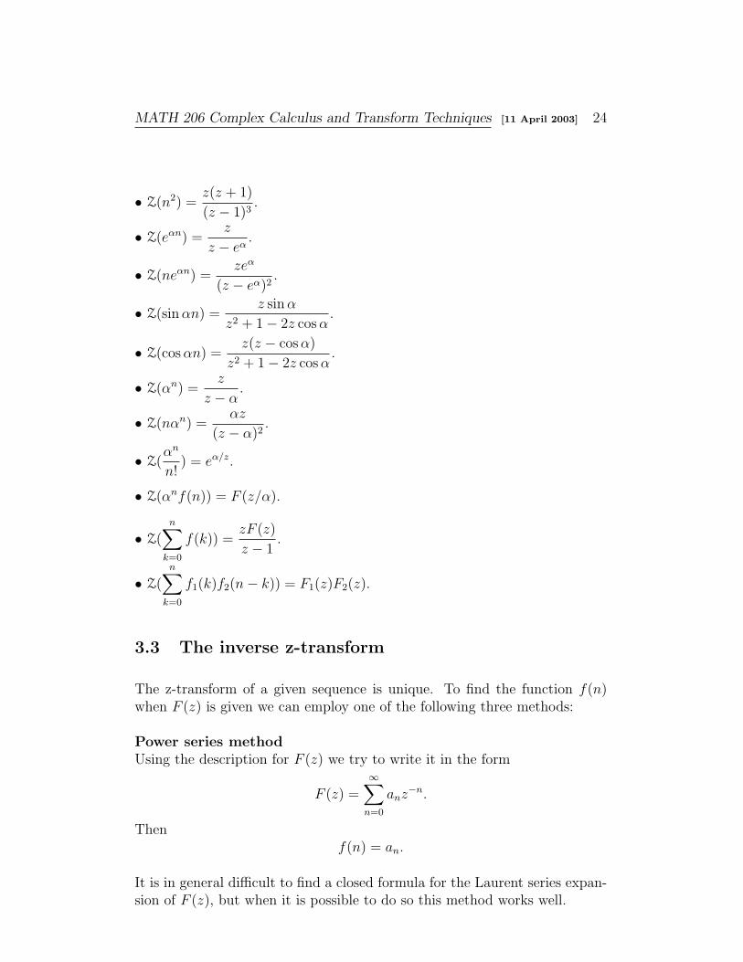
MATH 206 Complex Calculus and Transform Techniques [11 April 2003] 24
• Z(n2) =z(z + 1)
(z − 1)3.
• Z(eαn) =z
z − eα.
• Z(neαn) =zeα
(z − eα)2.
• Z(sin αn) =z sin α
z2 + 1− 2z cos α.
• Z(cos αn) =z(z − cos α)
z2 + 1− 2z cos α.
• Z(αn) =z
z − α.
• Z(nαn) =αz
(z − α)2.
• Z(αn
n!) = eα/z.
• Z(αnf(n)) = F (z/α).
• Z(n∑
k=0
f(k)) =zF (z)
z − 1.
• Z(n∑
k=0
f1(k)f2(n− k)) = F1(z)F2(z).
3.3 The inverse z-transform
The z-transform of a given sequence is unique. To find the function f(n)when F (z) is given we can employ one of the following three methods:
Power series methodUsing the description for F (z) we try to write it in the form
F (z) =∞∑
n=0
anz−n.
Thenf(n) = an.
It is in general difficult to find a closed formula for the Laurent series expan-sion of F (z), but when it is possible to do so this method works well.
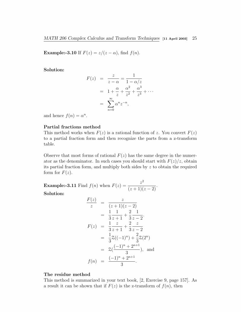
MATH 206 Complex Calculus and Transform Techniques [11 April 2003] 25
Example:-3.10 If F (z) = z/(z − α), find f(n).
Solution:
F (z) =z
z − α=
1
1− α/z
= 1 +α
z+
α2
z2+
α3
z3+ · · ·
=∞∑
n=0
αnz−n,
and hence f(n) = αn.
Partial fractions methodThis method works when F (z) is a rational function of z. You convert F (z)to a partial fraction form and then recognize the parts from a z-transformtable.
Observe that most forms of rational F (z) has the same degree in the numer-ator as the denominator. In such cases you should start with F (z)/z, obtainits partial fraction form, and multiply both sides by z to obtain the requiredform for F (z).
Example:-3.11 Find f(n) when F (z) =z2
(z + 1)(z − 2).
Solution:F (z)
z=
z
(z + 1)(z − 2)
=1
3
1
z + 1+
2
3
1
z − 2.
F (z) =1
3
z
z + 1+
2
3
z
z − 2
=1
3Z((−1)n) +
2
3Z(2n)
= Z((−1)n + 2n+1
3), and
f(n) =(−1)n + 2n+1
3.
The residue methodThis method is summarized in your text book, [2, Exercise 9, page 157]. Asa result it can be shown that if F (z) is the z-transform of f(n), then

MATH 206 Complex Calculus and Transform Techniques [11 April 2003] 26
f(n) =1
2πi
∫
C
zn−1F (z)dz
where C is a closed contour including the disk |z| ≤ R in its interior, where|z| > R is the region of convergence, or the region of analyticity, for thefunction F (z). This integral is then evaluated using residue theory. i.e.
f(n) =∑
Res(zn−1F (z)).
Example:-3.12 Find f(n) if its z-transform is F (z) = 4z/(3z2 − 2z − 1).
Solution: Resz=1
(zn−1F (z)) = 1, Resz=-1/3
(zn−1F (z)) = (−1/3)n−1. Sum of the
residues is 1 + (−1/3)n−1, which is the expression for f(n).
3.4 Solving difference equations
A difference equations is an equation of the form
a0f(n) + a1f(n + 1) + · · ·+ akf(n + k) = g(n, k)
where the ai’s are constants, g(n, k) is a given function, and we try to findf . These equations are also known as recurrence equations. Note that in theabove set up you must specify f(0), ..., f(k − 1) to find f .
To solve such an equation using z-transform, you take the z-transform ofboth sides of the equation to obtain an algebraic equation in F (z). You solvefor F (z) from this equation and take the inverse z-transform to find f .
Example:-3.13 Find a closed form expression for the general term of theFibonacci sequence which is defined by F1 = F2 = 1 and Fn + Fn+1 = Fn+2
for n ≥ 1.
Solution: We define f(n) = Fn+1 for n ≥ 0. Then recurrence equationbecomes f(n) + f(n + 1) = f(n + 2) with f(0) = f(1) = 1. Using the list ofelementary z-transforms we find that transforming both sides of this equationgives

MATH 206 Complex Calculus and Transform Techniques [11 April 2003] 27
F (z) + (zF (z)− z) = z2F (z)− z2 − z.
Solving this for F (z) we find
F (z) =z2
z2 − z − 1=
(φ
φ + 1/φ
)z
z − φ+
(1/φ
φ + 1/φ
)z
z + 1/φ
where φ =1 +
√5
2is the Golden Ratio. Applying inverse z-transform to
F (z) we find
f(n) =
(φ
φ + 1/φ
)(φ)n +
(1/φ
φ + 1/φ
)(−1
φ)n
=1√5
(φn+1 − (−1
φ)n+1
).
Since f(n) = Fn+1, we obtain the following closed form formula for thegeneral term of the Fibonacci sequence:
Fn =1√5
(φn −
(−1
φ
)n), for n > 2.
MATH 206 Complex Calculus and Transform Techniques [11 April 2003] 28
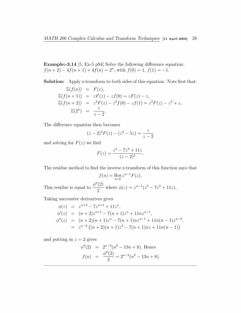
Example:-3.14 [5, Ex-5 p94] Solve the following difference equation:f(n + 2)− 4f(n + 1) + 4f(n) = 2n, with f(0) = 1, f(1) = −1.
Solution: Apply z-transform to both sides of this equation. Note first that:
Z(f(n)) = F (z),
Z(f(n + 1)) = zF (z)− zf(0) = zF (z)− z,
Z(f(n + 2)) = z2F (z)− z2f(0)− zf(1) = z2F (z)− z2 + z,
Z(2n) =z
z − 2.
The difference equation then becomes
(z − 2)2F (z)− (z2 − 5z) =z
z − 2
and solving for F (z) we find
F (z) =z3 − 7z2 + 11z
(z − 2)3.
The residue method to find the inverse z-transform of this function says that
f(n) = Resz=2
zn−1F (z).
This residue is equal toφ′′(2)
2where φ(z) = zn−1(z3 − 7z2 + 11z).
Taking successive derivatives gives
φ(z) = zn+2 − 7zn+1 + 11zn,
φ′(z) = (n + 2)zn+1 − 7(n + 1)zn + 11nzn−1,
φ′′(z) = (n + 2)(n + 1)zn − 7(n + 1)nzn−1 + 11n(n− 1)zn−2,
= zn−2((n + 2)(n + 1)z2 − 7(n + 1)nz + 11n(n− 1)
)
and putting in z = 2 gives
φ′′(2) = 2n−2(n2 − 13n + 8). Hence
f(n) =φ′′(2)
2= 2n−3(n2 − 13n + 8).

MATH 206 Complex Calculus and Transform Techniques [11 April 2003] 29
Example:-3.15 [4, Ex-5 p371] Solve the following difference equation:in+2 − in+1 + in = 0, where i1 = 3i0 − V/R and i0, V and R are constants.
Solution: Let I(z) denote the z-transform of in.
Z(in) = I(z),
Z(in+1) = zI(z)− zi0,
Z(in+2) = z2I(z)− z2i0 − zi1,
= z2I(z)− z2i0 − z(i0 − V/R).
The difference equation becomes
z2I(z)− z2i0 − z(3i0 − V/R)− 4zI(z) + 4zi0 + I(z) = 0
from which we find
I(z) =i0z
2 − (i0 + V
R
)z
z2 − 4z + 1.
The residue method to invert this is easier than the other methods. Thefunction I(z) has two simple poles at
z1 = 2−√
3 and
z2 = 2 +√
3.
An easy calculation gives
Resz = z1
zn−1I(z) =i0 + z1 −
(i0 + V
R
)
−2√
3zn1 , and
Resz = z2
zn−1I(z) =i0 + z2 −
(i0 + V
R
)
2√
3zn2 ,
Hence we get
in = Resz = z1
zn−1I(z) + Resz = z2
zn−1I(z), n ≥ 1
=i0 + z1 −
(i0 + V
R
)
−2√
3zn1 +
i0 + z2 −(i0 + V
R
)
2√
3zn2 ,
=i0
2√
3
((zn+1
2 − zn+11 ) + (zn
1 − zn2 )
)+
V
R
1
2√
3(zn
1 − zn2 )
= i0
‖n/2‖∑
k=0
(n + 12k + 1
)3k2n−2k −
‖(n−1)/2‖∑
k=0
(n
2k + 1
)3k2n−2k−1
−V
R
‖(n−1)/2‖∑
k=0
(n
2k + 1
)3k2n−2k−1
,
where ‖m‖ stands for the greatest integer which is less than or equal to m.
MATH 206 Complex Calculus and Transform Techniques [11 April 2003] 30
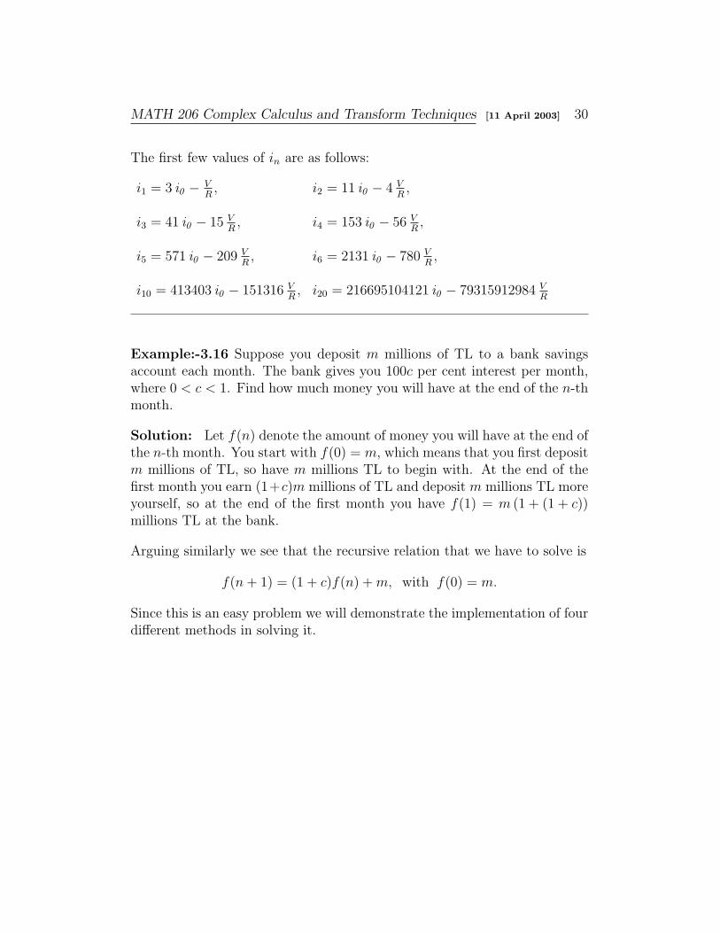
The first few values of in are as follows:
i1 = 3 i0 − VR, i2 = 11 i0 − 4 V
R,
i3 = 41 i0 − 15 VR, i4 = 153 i0 − 56 V
R,
i5 = 571 i0 − 209 VR, i6 = 2131 i0 − 780 V
R,
i10 = 413403 i0 − 151316 VR, i20 = 216695104121 i0 − 79315912984 V
R
Example:-3.16 Suppose you deposit m millions of TL to a bank savingsaccount each month. The bank gives you 100c per cent interest per month,where 0 < c < 1. Find how much money you will have at the end of the n-thmonth.
Solution: Let f(n) denote the amount of money you will have at the end ofthe n-th month. You start with f(0) = m, which means that you first depositm millions of TL, so have m millions TL to begin with. At the end of thefirst month you earn (1+c)m millions of TL and deposit m millions TL moreyourself, so at the end of the first month you have f(1) = m (1 + (1 + c))millions TL at the bank.
Arguing similarly we see that the recursive relation that we have to solve is
f(n + 1) = (1 + c)f(n) + m, with f(0) = m.
Since this is an easy problem we will demonstrate the implementation of fourdifferent methods in solving it.

MATH 206 Complex Calculus and Transform Techniques [11 April 2003] 31
Induction Method: Use induction to show that
f(n) =((1 + c)n+1 − 1
) m
c, for n = 0, 1, 2, ...
The next three methods involve the z-transform technique. Take the z-transform of the given recursion equation, solve for F (z) and find the inversez-transform of the solution. As usual we have
Z(f(n)) = F (z),
Z(f(n + 1)) = zF (z)− zf(0)
= zF (z)− zm,
Z(m) =mz
z − 1,
and the recursion equation becomes
zF (z)− zm = (1 + c)F (z) +mz
z − 1.
Solving this for F (z) gives
F (z) =z2
(z − 1)(z − (1 + c))m.
Now we will demonstrate the use of the three methods of inversion on thisfunction.
Power Series Method:
F (z) =z2
(z − 1)(z − (1 + c))m
=1
(1− 1/z)(1− (1 + c)/z)m
=
( ∞∑n=0
1
zn
)( ∞∑n=0
(1 + c)n
zn
)m
=∞∑
n=0
(n∑
k=0
(1 + c)k
)m
zn
=∞∑
n=0
[(1 + c)n+1 − 1]m
c
1
zn,
and hence the coefficient of 1/zn gives the required function f(n).

MATH 206 Complex Calculus and Transform Techniques [11 April 2003] 32
Partial Fractions Method:
F (z) =
[z
(z − 1)(z − (1 + c))
]zm
=
[−1
c
1
z − 1+
1 + c
c
1
z − (1 + c))
]zm
=
[−1
c
z
z − 1+
1 + c
c
z
z − (1 + c))
]m
= −m
cZ(1) +
(1 + c)m
cZ((1 + c)n)
= Z([(1 + c)n+1 − 1]m
c).
f(n) =[(1 + c)n+1 − 1]m
c.
Residue Method: We note that zn−1F (z) =zn+1m
(z − 1)(z − (1 + c)). Calcu-
lating its residues we find
Resz = 1
(zn−1F (z)
)= −m
c,
Resz = 1 + c
(zn−1F (z)
)=
(1 + c)n+1m
c.
Finally, adding up the residues we find the expected formula
f(n) =[(1 + c)n+1 − 1]m
c.
3.5 Unsorted exercises
These exercises are mostly taken from [4, 5, 8].Determine the z-transform of the following samples:
Exercise:-1 cosh αn. Ans:z2 − z cosh α
z2 − 2z cosh α + 1.
Exercise:-2 sinh αn. Ans:sinh α
z2 − 2z cosh α + 1.

MATH 206 Complex Calculus and Transform Techniques [11 April 2003] 33
Determine the inverse z-transform of the following functions:
Exercise:-3z
(z − 3)2. Ans: n(3n−1).
Exercise:-4z
z2 + 1. Ans: sin
nπ
2.
Exercise:-54z
4z2 − 2z√
3 + 1. Ans:
(1
2
)n−2
sinnπ
6.
Exercise:-62z3
(z − 2)3. Ans: (n2 + 3n + 2)2n.
Exercise:-7 z(e1/z − 1
). Ans: 1/(n + 1)!.
Exercise:-8 sinh2
z. Ans: (1− (−1)n)
2n−1
n!.
Solve the following difference equations:Exercise:-9 f(n + 1) + 2f(n) = (−1)n, with f(0) = −2.
Ans: f(n) = (−1)n − 3(−2)n.Exercise:-10 x(n + 2) + 5x(n + 1) + 6x(n) = 3, with x(0) = −2, x(1) = 1.
Ans: x(n) = (1/4)− 6(−2)n + (15/4)(−3)n.Exercise:-11 2f(n + 3) − 3f(n + 2) + f(n) = 0, with f(0) = 0, f(1) = 1,f(2) = −4. Ans: f(n) = −(8/3)(−1/2)n + (8/3)− 3n.Exercise:-12 x(n + 2)− 2x(n + 1) + x(n) = 0, with x(0) = A, x(1) = B.
Ans: x(n) = A + (B − A)nExercise:-13 y(n + 2)−
√3y(n + 1) + y(n) = 0, with y(0) = 1, y(1) =
√3.
Ans: y(n) = cos(nπ/6) +√
3 sin(nπ/6).Exercise:-14 a(n + 2)− 5a(n + 1) + 6a(n) = 1, with a(0) = 2, a(1) = 3.
Ans: a(n) = (1− 3n + 2n+2)/2.

MATH 206 Complex Calculus and Transform Techniques [11 April 2003] 34
References
[1] Bolton, W., Laplace & z-transforms, Longman Scientific & Technical,1994.
[2] Brown, J.W., Churchill, R.V., Complex Variables and Applications,McGraw-Hill International, 6th ed., 1996.
[3] Churchill, R.V., Operational Mathematics, McGraw-Hill, 1972.
[4] Fisher, S. D., Complex Variables, Second Edition, Wadsworth & Brooks,1990.
[5] Grove, A.C., Laplace transform and the z-transform, Prentice Hall, 1991.
[6] Osborne, A.D., Complex Variables and Their Applications, Addison-Wesley, 1999.
[7] Ross, S.L., Differential Equations, John Wiley & Sons, 3rd ed., 1984.
[8] Saff, E. B., Snider, A. D., Complex Analysis, Prentice Hall, PearsonEducation Inc., 2003.
[9] Spiegel, M.R., Laplace Transforms, Schaum’s outline series, McGraw-Hill, 1990.