Embed Size (px)
Citation preview

Lecture notes in Computability Theory A. Miller December 3, 2008 1
Lecture notes in Computability TheoryArnold W. Miller
These are lecture notes from Math 773. There were mostly written in2004 but with some additions in 2007.
DESCRIPTION: Abstract theory of computation. Turing degree and jump,arithmetic hierarchy, index sets, simple and (hyper)hypersimple sets, Kleene-Post results in Turing degrees, finite injury priority arguments: Friedberg-Muchnik Theorem, Sacks Splitting Theorem, existence of a maximal set.Infinite injury priority arguments: Lachlan minimal pair, Sacks density the-orem, Shoenfield incomplete high degrees. Recursive ordinals and the hyper-arithmetical hierarchy.
Some general references in this area are:Hartley Rogers, Theory of recursive functions, 1967Robert Soare, Recursively enumerable sets and degrees, 1987Piergiorgio Odifreddi, Classical recursion theory, vol 1,2 1989,1999Barry Cooper, Computability theory, 2004Robert Soare, Computability theory and applications, 2008
Contents
1 UR-Basic programming 3
2 Primitive recursive functions 6
3 Primitive recursive functions are UR-Basic computable 11
4 UR-BASIC computable functions are recursive 12
5 Church-Turing Thesis 16
6 Universal partial computable function 18
7 The computably enumerable sets 19
8 Separation and reduction 23

Lecture notes in Computability Theory A. Miller December 3, 2008 2
9 Many-one reducibility 24
10 Rice’s index Theorem 26
11 Myhill’s computable permutation Theorem 27
12 Roger’s adequate listing Theorem 30
13 Kleene’s Recursion Theorem 31
14 Myhill’s characterization of creative set 33
15 Simple sets 36
16 Oracles 37
17 Dekker deficiency set 37
18 Turing degrees and jumps 38
19 Kleene-Post: incomparable degrees 39
20 The join 41
21 Meets 42
22 Spector: exact pairs 44
23 Friedberg: jump inversion 46
24 Spector: minimal degree 48
25 Sacks: minimal upper bounds 50
26 Friedberg-Muchnik Theorem 51
27 Embedding in the c.e. degrees 55
28 Limit Lemma and Ramsey Theory 56
29 A low simple set 58

Lecture notes in Computability Theory A. Miller December 3, 2008 3
30 Friedberg splitting Theorem 61
31 Sacks splitting Theorem 62
32 Lachlan and Yates: minimal pair 68
33 Friedberg: A one-one enumeration of the c.e. sets 74
34 Hypersimple sets 79
35 Hyperhypersimple sets 85
36 Maximal sets 88
37 The lattice of c.e. sets 91
38 Arithmetic hierarchy 99
39 Post: ∆02 same as computable in 0′ 101
40 EMP, TOT, FIN, and REC 104
41 Domination and high degrees 109
42 High degrees using the Psuedojump 112
43 First-order theories 117
44 Analytic sets 120
Appendix
45 Turing machines 130
46 Trees, Konig’s Lemma, Low basis 136
1 UR-Basic programming
We begin by giving a formal definitions of computability, a toy programminglanguage: UR-BASIC.

Lecture notes in Computability Theory A. Miller December 3, 2008 4
Variables are any string of letters or numerals, A-Za-z0-9.Statements are of the form
Let X = X + 1Let X = X−1If X ≤ Y then goto k
where X and Y are any variables and k is a nonnegative integer, i.e. k ∈ ω,which is a line number.
A UR-Basic program is a sequence S0, S1, S2, . . ., Sn of statements.Variables only take on nonnegative integer values. The symbol − meanssubtraction unless the result is negative and then it yields zero. The programhalts if we “goto” to a line k > n.
A function f : ω → ω is UR-Basic computable iff there exists a programP , designated input variable X and output variable Y such that for anyn ∈ ω if we put X = n and all other variables zero and start with the firststatement of P , then P eventually halts with f(n) in variable Y . There is asimilar definition for f : ωm → ω to be UR-Basic computable.
Next we indicate how to simulate more complex statements using thesethree kinds of statements. When substituting multiline statements for asingle statement, the “goto” numbers must be adjusted.
Basic: UR-Basic:Go to k If X ≤ X then goto kContinue Let Donothing=Donothing+1
Let Y=X 1 If X ≤ Y then go to 42 Let Y=Y+13 Go to 14 If Y ≤ X then go to 75 Let Y = Y −16 Go to 47 Continue
Constants0 this is a variable - we agree never to change it1 let 1 = 1 + 1
2 Let 2 = 2 + 1Let 2 = 2 + 1

Lecture notes in Computability Theory A. Miller December 3, 2008 5
If X < Y then goto k Let tempX = XLet tempX = tempX + 1if tempX ≤ Y then goto k
If X = Y then goto k 1 If X < Y then goto 42 If Y < X then goto 43 Go to k4 continue
For i = 1 to n 1 If n = 0 then goto 7S1 2 Let i = 1. . . 3 S1
Sk . . .Next i 4 Sk
5 Let i = i+ 16 If i ≤ n then goto 37 continue
Example 1.1 The pair of functions remainder and quotient are UR-Basiccomputable i.e., input n,m then output q, r with n = qm+ r and 0 ≤ r < m.
Proofn = qm+ r:
1 Let q = 02 Let r = n3 If r < m then goto 74 Let r = r−m5 Let q = q + 16 go to 37 continue
QED
Example 1.2 The functions Z = X + Y , Z = XY , Z = XY , and X−Yare UR-Basic computable.

Lecture notes in Computability Theory A. Miller December 3, 2008 6
ProofZ = X + Y :
Let Z = XFor i = 1 to Y
Let Z = Z + 1Next i
Z = XY :Let Z = 0For i = 1 to Y
Let Z = Z +XNext i
Z = XY :Let Z = 1For i = 1 to Y
Let Z = ZXNext i
Z = X−Y :Let Z = XFor i = 1 to Y
Let Z = Z−1Next i
QED
Exercise 1.3. Prove that the greatest common divisor function d =gcd(n,m) is UR-Basic computable. Or if you prefer the function f(n) =the nth prime. Or you can prove that your favorite function is UR-Basiccomputable.
2 Primitive recursive functions
The class of primitive recursive functions is the smallest set of functionsf : ωm → ω of arbitrary arity m which contain
1. the constant zero function, Z : ω → ω, Z(n) = 0 all n,

Lecture notes in Computability Theory A. Miller December 3, 2008 7
2. the successor function, S : ω → ω with S(n) = n + 1 all n (which weusually write n+ 1), and
3. the projections πnm(x1, . . . , xn) = xm for 1 ≤ m ≤ n < ω
and is closed under
• composition: h is primitive recursive, if
h(x1, . . . , xm) = f(g1(x1, . . . , xm), . . . , gn(x1, . . . , xm))
where f is n-ary and each gi is m-ary are primitive recursive, and
• primitive recursion: h is primitive recursive, if
h(0, x1, . . . , xm) = g(x1, . . . , xm)
h(y + 1, x1, . . . , xm) = f(y, x1, . . . , xm, h(y, x1, . . . , xm))
where g is m-ary and f is (m+ 2)-ary primitive recursive.
Note that by using the projections and compositions we may swap vari-ables around and introduce dummy variables, e.g.
h(x, y, z) = f(g(x, y), z, k(z, x)) = f(g1(x, y, z), g2(x, y, z), g3(x, y, z))
where
g1(x, y, z) = g(π31(x, y, z), π
32(x, y, z))
g2(x, y, z) = π33(x, y, z)
g3(x, y, z) = k(π33(x, y, z), π
32(x, y, z))
A predicate P ⊆ ωn is primitive recursive iff its characteristic functionχP (~x) is where
χP (~x) =
1 if P (~x)0 if ¬P (~x)
Constant functions of any arity are primitive recursive. E.g., the functionf(x, y, z) = 2 for all x, y, z is defined by
f(x, y, z) = S(S(Z(π31(x, y, z))))
Define z = x+ y:

Lecture notes in Computability Theory A. Miller December 3, 2008 8
x+ 0 = xx+ (y + 1) = (x+ y) + 1
Define z = xy:x0 = 0x(y + 1) = xy + x
Define z = xy:x0 = 1xy+1 = xyx
Define z = x(y) = xxx.x
:x(0) = xx(y+1) = xx
(y)
Define z = x!:0! = 1(x+ 1)! = (x+ 1)x!
Define z = x−1:0−1 = 0(x+ 1)−1 = x
Define z = y−x:y−0 = yy−(x+ 1) = (y−x)−1
Define
sign(x) =
1 if x > 00 if x = 0
by sign(x) = 1−(1−x).
Proposition 2.1 The predicates x ≤ y, x = y, x < y are primitive recur-sive. If P and Q are primitive recursive predicates, then so is P ∨Q and ¬P .If P (~x, y) is a primitive recursive predicate and f(~x) a primitive recursivefunction, then Q(~x) ≡ P (~x, f(~x)) is a primitive recursive predicate.

Lecture notes in Computability Theory A. Miller December 3, 2008 9
Proofχ≤(x, y) = 1−(x−y)χP∨Q = sign(χP + χQ)χ¬P = 1−χPx = y iff x ≤ y and y ≤ xx < y iff ¬y ≤ xχQ(~x) = χP (~x, f(~x))
QED
Proposition 2.2 If P (~x, y) is a primitive recursive predicate and f(~x) aprimitive recursive function, then
∃y ≤ f(~x) P (~x, y) and ∀y ≤ f(~x) P (~x, y)
are both primitive recursive predicates.
ProofLet
Q(~x, z) ≡ ∃y ≤ z P (~x, y)
Then χQ has the recursive definition:χQ(~x, 0) = χP (~x, 0)χQ(~x, z + 1) = sign(χQ(~x, z) + χP (~x, z + 1))
Note thatQ(~x, h(~x) ≡ ∃y ≤ h(~x) P (~x, y)
and
∀y ≤ h(~x) P (~x, y) ≡ ¬∃y ≤ h(~x) ¬P (~x, y)
QEDFor example,
x divides y iff ∃z ≤ y y = xz.x is a Prime iff x > 1 and ∀y ≤ x if y divides x, then y = 1 or y = x.
are primitive recursive predicates.
Bounded search: define f(~x, z) = µy ≤ z P (~x, y) where f is the least y ≤ zwhich satisfies P (~x, y) and f = 0 if no y ≤ z can be found.

Lecture notes in Computability Theory A. Miller December 3, 2008 10
Proposition 2.3 Suppose Q is a primitive recursive predicate and h a prim-itive recursive function. Then
g(~x) = µy ≤ h(~x) P (~x, y)
is primitive recursive.
ProofLet
Q(~x, y) ≡ P (~x, y) ∧ ∀u < y ¬P (~x, u).
Then if we definef(~x, z) = µy ≤ z P (~x, y)
then
f(~x, z) =z∑y=0
y · χQ(~x, y)
which has the following primitive recursive definition:f(~x, 0) = 0f(~x, z + 1) = f(~x, z) + (z + 1)χQ(~x, z + 1)
Henceg(~x) = f(~x, h(~x)) = µy ≤ h(~x) P (~x, y).
QED
Proposition 2.4 If f : ω → ω is primitive recursive, the graph(f) is a prim-itive recursive predicate. If graph(f) is a primitive recursive predicate andthere is a primitive recursive function g which bounds f , then f is primitiverecursive.
ProofGraph(f) has characteristic function χ=(f(~x), y). If f is bounded by g then
f(~x) = µy ≤ g(~x) (~x, y) is in the graph of f.
QEDExamples:
z=max(x,y) iff (x = z and x ≥ y) or (y = z and y ≥ x)has primitive recursive graph and is bounded by x + y, so it is a primitiverecursive function.

Lecture notes in Computability Theory A. Miller December 3, 2008 11
Division,Quotient: input n,m > 0 output q, r with n = qm+r and r < m.q = quotient(n,m) and r = remainder(n,m) both have primitive recursivegraphs bounded by n+m so they are primitive recursive.
Exercise 2.5. Let r(n) = nth digit of√
2 = 1.4142136 . . ., so r(0) = 1,r(1) = 4, and so on. Prove that r is primitive recursive. If you prefer youmay use e = 2.7182818 . . . instead of
√2. Does every naturally occurring
constant in analysis have this property?
Exercise 2.6. Define n is square-free iff n ≥ 2 and no m2 divides n form ≥ 2. Let S(n) be the sum of the first n square-free numbers. Prove S isa Primitive recursive function.
3 Primitive recursive functions are UR-Basic
computable
Theorem 3.1 Every primitive recursive function is UR-Basic computable.
ProofThe empty program with input x and output y, computes the constant zerofunction. Similarly for the projections. The successor function is computedby the one-line program “Let x=x+1”, with input and output variable x.
For closure under composition: z = f(g1(~x), . . . , gn(~x)) use the basicprogram:
Let z1 = g1(~x)Let z2 = g2(~x)· · ·Let zn = gn(~x)Let y = f(z1, . . . , zn)
where appropriate substitution of UR-Basic code has been done.
The basic code for a primitive recursive definitionf(~x, 0) = g(~x)f(~x, n+ 1) = h(n, f(~x, n), ~x)
looks likeinput ~x, nLet y = g(~x)

Lecture notes in Computability Theory A. Miller December 3, 2008 12
For i = 1 to nLet y = h(i−1, y, ~x)
next ioutput y = f(~x, n)
QED
4 UR-BASIC computable functions are re-
cursive
Definition 4.1 The partial recursive functions are the smallest class of func-tions containing the primitive recursive functions and closed under composi-tion, primitive recursion, and unbounded search µ:
f(~x) = µy P (~x, y)
where P is a recursive predicate,i.e., its characteristic function is recursive.
Theorem 4.2 (Kleene) There exists a primitive recursive predicate Q andprimitive recursive g such that for every partial UR-Basic computable f :ω → ω there exists an e such that
∀x f(x) = g(µz Q(e, x, z)).
ProofAn informal description of g and Q are as follows. Q(e, x, z) says that theprogram coded by e with input x does the computation coded by z. g(z) isthe value of the output variable at the final step of the computation codedby z.
In order to more formally define Q we begin by describing a method ofcoding pairs and finite sequences using primitive recursive functions.Coding pairs. the mapping x, y 7→ 〈x, y〉 defined by
〈x, y〉 = 2x(2y + 1)− 1
is a primitive recursive bijection between ω2 and ω. Both unpairing functionsare primitive recursive since if x = 〈x0, x1〉, then x0, x1 ≤ x. So define thehead and tail functions h and t as follows:
h(〈x, y〉) = x and t(〈x, y〉) = y
Lecture notes in Computability Theory A. Miller December 3, 2008 13
Triples can be coded by 〈x, y, z〉 = 〈x, 〈y, z〉〉 and similarly by induction forn-tuples:
〈x1, x2, . . . , xn〉 = 〈x1, 〈x2, . . . , xn〉〉.Note that, for example,
h(t(t(〈x, y, z, w〉))) = z
so the “coordinate function” 〈x, y, z, w〉 7→ z is primitive recursive.To code finite sequences of arbitrary length define the function
c(y, k) = h(t(k)(y))
where t(k) stands for the composition of t with itself k times. It has a primitiverecursive definition f(k, x) = t(k)(x):
f(x, 0) = x
f(x, k + 1) = t(f(x, k))
It is easy to check that c has the property that for any n and for any finitesequence y0, y1, . . . , yn there exists y such that c(y, k) = yk for all k ≤ n. Weoften use yi to denote c(y, i)
We can assume that the UR-Basic program only uses the variable vi fori < ω and that the input variable is v0 and output variable v1.
1. S = 〈0, i〉 ∈ ω codes the statement “Let vi = vi + 1”.2. S = 〈1, i〉 ∈ ω codes the statement “Let vi = vi−1”.3. S = 〈n, i, j, k〉 for n ≥ 2 codes the statement “If vi ≤ vj then goto k”.
For e ∈ ω let e = 〈n, S〉 and let S0, S1, . . . , Sn−1 be the program statementswith Si coded by c(S, i).
Next we define three primitive recursive predicates:In the tuple (e, x, y), e codes the program, x is the input value and y is
pair 〈k, V 〉 coding the line k in the program which is being executed and Vcoding the values of the variables.
Init(e, x, y) ≡∃V < y y = 〈0, V 〉 and c(V, 0) = x and ∀i < e (i > 0→ c(V, i) = 0)
Since this is the start we want to start with Statement 0, i.e., y = (0, V )and v0 = x and vi = 0 for all i with 0 < i < e. Note that we can bound thisby e since e cannot refer to any variables with index higher than e.

Lecture notes in Computability Theory A. Miller December 3, 2008 14
Halt(e, y) ≡
∃n, S < e ∃k, V < y y = 〈k, V 〉 and e = 〈n, S〉 and k ≥ n
All this says is we halt when we try to execute a line number greater thanthe length of the program.
Onestep(e, y, y′) ≡
(This says we take one step from y to y′.)
∃k, V, k′, V ′ < y + y′ and ∃n, S < e such that all of the following are true:
1. y = 〈k, V 〉, y′ = 〈k′, V ′〉, and e = 〈n, S〉
2. k < n (we don’t take a step if program has halted)
3. If c(S, k) codes “Let vi = vi + 1” then
c(V ′, i) = c(V, i) + 1,
c(V ′, j) = c(V, j) for all j < e with j 6= i, and
k′ = k + 1,
4. If c(S, k) codes “Let vi = vi−1” then
c(V ′, i) = c(V, i)−1,
c(V ′, j) = c(V, j) for all j < e with j 6= i, and
k′ = k + 1.
5. If c(S, k) codes “If vi ≤ vj then goto l” then
V = V ′ and
if c(V, i) ≤ c(V, j) then k′ = l else k′ = k + 1.
Next we define the predicate Q(e, x, z). Informally, it says that z codes acomputation using program e and input x.
Q(e, x, z) ≡
∃N, y < z z = 〈N, y〉 and Init(e, x, c(y, 0)) and Halt(e, c(y,N)) and
∀i < N Onestep(e, c(y, i), c(y, i+ 1))

Lecture notes in Computability Theory A. Miller December 3, 2008 15
Finally we define the function g. It simply extracts the value of v1 theoutput variable from the computation coded by z. Since g(z) ≤ z it is enoughto see that its graph is primitive recursive:
g(z) = v iff
∃N, y, V, k < z 〈N, y〉 = z and c(y,N) = 〈k, V 〉 and c(V, 1) = v
QED
Corollary 4.3 The family of (partial) UR-Basic computable functions is thesame as the family of (partial) recursive functions.
ProofThe family of UR-Basic computable functions is closed under unboundedsearch µ, i.e.,
To compute the function f(~x) = µy P (~x, y) use code:
1 Let y = 02 If P (~x, y) then goto 53 Let y = y + 14 Goto 25 continue
Hence every partial recursive function is partial UR-Basic computable.The Theorem supplies the other inclusion.QED
The Theorem shows that only one unbounded search is needed to getevery partial recursive function. Something that is not immediately evidentfrom the definition of recursive function.
Exercise 4.4. Another way to code finite sequences of arbitrary length isto use prime factorization.
(a) Define: nextprime(x) = y to be the smallest prime y > x. Prove thatnextprime(x) is primitive recursive.
(b) Define: p0 = 2 and pn is the nth odd prime. Prove that the functionn 7→ pn is primitive recursive.
(c) Define c(x, i) = k iff k is the least integer such that pk+1i does not
divide x. Prove that c is primitive recursive and for any finite sequencex0, x1, . . . , xn there exists x such that c(x, k) = xk for all k ≤ n.

Lecture notes in Computability Theory A. Miller December 3, 2008 16
Exercise 4.5. Suppose that f : ω → ω is UR-Basic computable by aprogram P and there exists a primitive recursive function s : ω → ω suchthat for every x the program P computes f(x) in ≤ s(x) steps. Prove thatf is primitive recursive.
Exercise 4.6. The programming language P-Basic has only four kinds ofstatements
(a) Let X = X + 1(b) Let X = X−1(c) Let X = Y
where X, Y are any variables(d) for-next loops, e.g.
For i = 1 to nS1...Sk
Next i
The loop variable i and n must be distinct and in the body of the loop(S1, . . . , Sk) the variables i and n are not allowed to be changed, i.e.,
For n= 1 to . . .For i= 1 to . . .Let n = . . .Let i = . . .
are not allowed. Prove that the P-Basic computable functions are the sameas the primitive recursive functions.
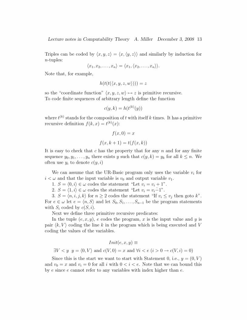
Exercise 4.7 Another popular pairing function p : ω2 → ω is described byFigure 1. Show that p is a polynomial. Hint: the point (m,n) is on thediagonal of the square of area (m+ n)2.
5 Church-Turing Thesis
Church-Turing Thesis:
Every intuitively computable function is recursive.
Lecture notes in Computability Theory A. Miller December 3, 2008 17
6
-r r r rr r rr rr
@@@I
@@@I
@@@I
@@@I
@@@I
@@@I
0 1 3 6
2
5
9
4 7
8 = p(1, 3)
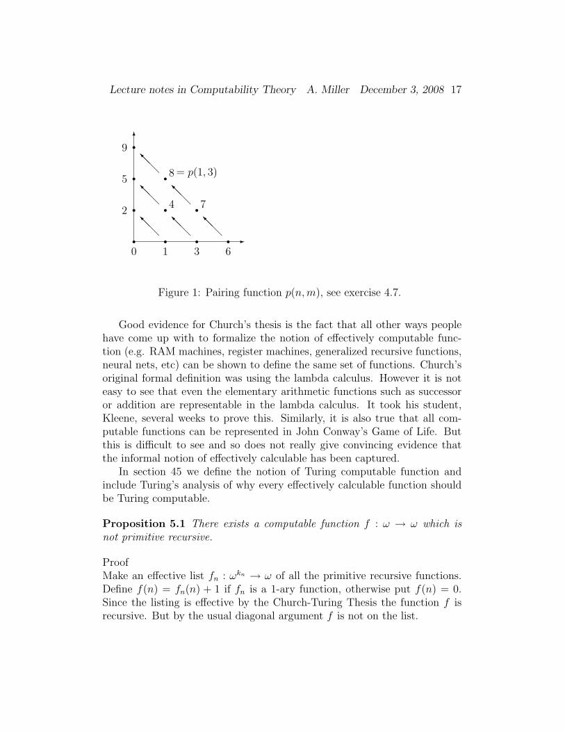
Figure 1: Pairing function p(n,m), see exercise 4.7.
Good evidence for Church’s thesis is the fact that all other ways peoplehave come up with to formalize the notion of effectively computable func-tion (e.g. RAM machines, register machines, generalized recursive functions,neural nets, etc) can be shown to define the same set of functions. Church’soriginal formal definition was using the lambda calculus. However it is noteasy to see that even the elementary arithmetic functions such as successoror addition are representable in the lambda calculus. It took his student,Kleene, several weeks to prove this. Similarly, it is also true that all com-putable functions can be represented in John Conway’s Game of Life. Butthis is difficult to see and so does not really give convincing evidence thatthe informal notion of effectively calculable has been captured.
In section 45 we define the notion of Turing computable function andinclude Turing’s analysis of why every effectively calculable function shouldbe Turing computable.
Proposition 5.1 There exists a computable function f : ω → ω which isnot primitive recursive.
ProofMake an effective list fn : ωkn → ω of all the primitive recursive functions.Define f(n) = fn(n) + 1 if fn is a 1-ary function, otherwise put f(n) = 0.Since the listing is effective by the Church-Turing Thesis the function f isrecursive. But by the usual diagonal argument f is not on the list.

Lecture notes in Computability Theory A. Miller December 3, 2008 18
QED
Exercise 5.2. Prove that there exists a (total) h : ω → ω whose graphis a primitive recursive predicate but h is not a primitive recursive function.Hint: consider h(x) = µz Q(e, x, z).
Exercise 5.3. Prove there exists a primitive recursive bijection p : ω → ωsuch that p−1 is not primitive recursive.
6 Universal partial computable function
Proposition 6.1 (Turing) There exists a universal partial computable func-tion
ψ : ω → ω
i.e. if we define ψe(x) = ψ(〈e, x〉) then ψe : e ∈ ω is a uniformlycomputable listing of all partial computable functions.
Proofψ(〈e, x〉) = g(µz Q(e, x, z)).QED
Note that for any n ≥ 2 if f(x1, . . . , xn) is a partial computable functionthen there will be e such that
∀x1, . . . , xn ψ(〈e, 〈x1, . . . , xn〉〉) = f(x1, . . . , xn).
So ψ is universal for partial computable functions of any arity.
Proposition 6.2 (Padding Lemma) There exists a 1-1 computable functionp such that ψe = ψp(e,n) for every e, n.
ProofTo pad the program S0, S1, . . . , Sm coded by e just add the statement
Sm+1 = LetDonothing〈e, n〉 = Donothing〈e, n〉+ 1
and let p(e, n) code this new program.QED
Proposition 6.3 (S-n-m Theorem). There exists a computable function Ssuch that ψe(〈x, y〉) = ψS(e,x)(y) for all e, x, y.
Lecture notes in Computability Theory A. Miller December 3, 2008 19
ProofGiven P the program coded by e and input x make-up a new program codedby S(e, x) which puts x into P ’s first input variable and then pops intoprogram P .QED
The name S-n-m comes from the obvious generalization to n-tuple ~x andm-tuple ~y
ψe(〈~x, ~y〉) = ψSn,m(e,~x)(~y)
so what we are stating is the S-1-1 Theorem.These propositions can be combined as follows:
Proposition 6.4 Suppose θ(x, y) is a partial computable function. Thenthere is a one-to-one computable function f : ω → ω such that
∀x, y ψf(x)(y) = θ(x, y).
ProofSuppose θ = ψe0 . Then
θ(x, y) = ψp(S(e0,x),x)(y)
and so f(x) = p(S(e0, x), x) works.QED
We call this the 1-1-S-1-1 Theorem.
7 The computably enumerable sets
Definition 7.1 For A ⊆ ω define:
1. A is computably enumerable iff either A is empty or A is the rangeof a computable function, i.e., A = a0, a1, a2, . . . where the functionn 7→ an is computable. This is abbreviated c.e.
2. A is Σ01 iff there exists a computable predicate R ⊆ ω2 such that
A = n : ∃m R(n,m).
Definition 7.2 W = 〈e, x〉 : ψ(〈e, x〉) ↓. Then We : e ∈ ω whereWe = x : 〈e, x〉 ∈W is a uniform listing of the c.e. sets.

Lecture notes in Computability Theory A. Miller December 3, 2008 20
Proposition 7.3 For A ⊆ ω the following are equivalent:(1) A is computably enumerable.(2) A is the domain of a partial computable function.(3) A is Σ0
1.(4) A is finite or A has a one-to-one computable enumeration.(5) There exists e such that A = We.
Proof(1) → (2): Given a computable enumerable listing an describe a partial
computable function f by:
• input x
• look for x on the list: a0, a1, a2, . . .
• halt if you find it, otherwise continue looking forever.
(2)→ (1): Define ψe,s(x) ↓= y to mean that
e, x, y < s ∧ ∃z < s (Q(e, x, z) ∧ g(z) = y).
See Theorem 4.2. The predicate
P (e, x, y, s) ≡ ψe,s(x) ↓= y
is primitive recursive. It roughly says that the algorithm coded by e withinput x terminates in fewer than s steps and outputs y. (Actually z is asequence coding the values of the variables and the line number at eachstep.) If A is the domain of ψe, then either A is empty or let x0 ∈ A bearbitrary and define a recursive enumeration of A by
an =
x if n = 〈x, y, s〉 and ψe,s(x) ↓= yx0 otherwise.
(1) → (3): Let f : ω → ω be computable and have range A. Let R bethe graph of f , then y ∈ A iff ∃x R(x, y).
(3) → (2): Suppose x ∈ A iff ∃y R(x, y). Then f(x) = µy R(x, y) ispartial recursive with domain A.
(1) → (4): Given an : n < ω a computable enumeration of A, definea computable enumeration bn : n < ω by:
bn+1 = am where m is the least such that am /∈ bi : i ≤ n.(2)↔ (5): by definition.
QED

Lecture notes in Computability Theory A. Miller December 3, 2008 21
Definition 7.4 For A ⊆ ω, define:
1. A is computable iff its characteristic function χA is computable.
2. A = ω \ A the complement of A,
3. A is Π01 iff A is Σ0
1, and
4. ∆01 = Σ0
1 ∩ Π01.
Proposition 7.5 For A ⊆ ω the following are equivalent:(1) A is computable.(2) A and A are both computably enumerable.(3) A is ∆0
1.(4) A is finite or A has a strictly increasing computable enumeration.
Proof(1)→ (2): It is easy to see that computable implies computably enumer-
able and that the complement of a computable set is computable.(2)→ (1): Input x. Effectively list A and A simultaneously until x shows
up.(2) iff (3): Trivial.(1)→ (4): Take an to be the nth element of A.(4) → (1): Let an : n < ω be a strictly increasing computable enu-
meration of A. The following algorithm computes the characteristic functionof A:
• Input x.
• Find n such that an > x.
• Then x ∈ A iff x ∈ ai : i < n.
QED
Example 7.6 There exists a c.e. set K which is not computable.
ProofK = e : ψe(e) ↓
If K is the domain of ψe, then e ∈ K iff e /∈ K.QED

Lecture notes in Computability Theory A. Miller December 3, 2008 22
Proposition 7.7 Every infinite c.e. set contains an infinite computable set.
ProofGiven an : n < ω a computable enumeration of A, define a strictlyincreasing computable enumeration bn : n < ω by:
b0 = a0 andbn+1 = am where m is the least such that am > bn.
QED
Proposition 7.8 If A and B are c.e. sets, then A ∩ B is c.e. and A ∪ Bis c.e. If A and B are computable sets, then A ∩ B, A ∪ B, and A are allcomputable sets.
ProofDomain of f + g is the intersection of domain f and domain g. EnumerateA ∪B by x2n = an and x2n+1 = bn.QED
Exercise 7.9. Suppose that V ⊆ ω is c.e. For each n define Vn = x :〈n, x〉 ∈ V . Prove that ∪nVn is c.e.
Exercise 7.10. Prove that every nonempty computably enumerable setA is the range of a primitive recursive function. Extra Credit: prove thatnot every infinite computably enumerable set is the range of a one-to-oneprimitive recursive function.
Exercise 7.11. (a) For a partial function f : ω → ω prove that f is partialcomputable iff its graph is computably enumerable.
(b) For a partial computable h prove there is a partial computable g withdom(g) ⊇ range(h) such that
∀y ∈ range(h) h(g(y)) = y.
(c) Give an example for (b) for which g cannot be total.
Exercise 7.12. Consider a partial function f : ω → ω and the three set:
1. dom(f) ⊆ ω
2. graph(f) ⊆ ω × ω

Lecture notes in Computability Theory A. Miller December 3, 2008 23
3. range(f) ⊆ ω.
For each of the sets (1), (2), (3) could be:(a) computable or(b) computably enumerable but not computable.
For each of the 8 possibilities, either give an example of such an f or provethere is no such f . Extra credit: consider the third possibility (c) not com-putably enumerable.
Exercise 7.13. If f : ω → ω, then fn denotes f applied n times; e.g.,f 3(0) = f(f(f(0))). Give an example of a (total) computable f such thatfn(0) : n ∈ ω is not computable.
Exercise 7.14. Define Ve = x : 〈e, x〉 ∈ V . Prove or disprove:
1. ∃V computably enumerable such that Ve : e ∈ ω is the set of allcomputable sets.
2. ∃V computable such that Ve : e ∈ ω is the set of all computable sets.
3. ∃V c.e. such Ve : e ∈ ω is the set of all nonempty c.e. sets.
4. ∃f a computable function such that for all e We 6= ∅ implies f(e) ∈We.
5. ∃f partial computable such that for all e We 6= ∅ implies f(e) ↓∈ We.
Exercise 7.15 Prove there exists a computable function f : ω → ω suchthat for every e
We infinite → (ψf(e) : ω → We is total, one-to-one, and onto).
For the definition of We see Definition 7.2.
8 Separation and reduction
Example 8.1 There exists disjoint c.e. sets K0 and K1 which are com-putably inseparable, i.e., there is not exists a computable set R ⊆ ω withK0 ⊆ R and K1 ⊆ R.

Lecture notes in Computability Theory A. Miller December 3, 2008 24
ProofK0 = e : ψe(e) ↓= 0 and K1 = e : ψe(e) ↓= 1
QED
Definition 8.2 For any Γ ⊆ P (ω) define Γ to be the set of all A for A ∈ Γ
and define ∆ = Γ ∩ Γ. Sep(Γ) is the property that for every A,B ∈ Γdisjoint there exists C ∈ ∆ with A ⊆ C and B ⊆ C. Red(Γ) (the reductionprinciple) is the property that for every A,B ∈ Γ there exists disjoint A′ ⊆ Aand B′ ⊆ B with A′, B′ ∈ Γ and A ∪B = A′ ∪B′.
Proposition 8.3 Red(Γ) implies Sep(Γ).
ProofApply reduction to the complements.QED
Proposition 8.4 Red(Σ01) and hence Sep(Π0
1).
ProofA = x : ∃u R(u, x) and B = x : ∃v S(v, x). Put
x ∈ A′ ↔ ∃u R(u, x) and ∀v ≤ u¬S(v, x)
x ∈ B′ ↔ ∃v S(v, x) and ∀u < v¬R(u, x)
QEDIn example 8.1 it follows that K0 and K1 cannot be separated by disjoint
Π01 sets B0 and B1 because such a B0 and B1 could be computably separated.
Exercise 8.5. Prove Sep(Γ) for Γ = A ∪B : A ∈ Σ01, B ∈ Π0
1.
9 Many-one reducibility
Definition 9.1 For A,B ⊆ ω define:
1. A ≤m B iff there exists a computable function f such that
∀x ∈ ω x ∈ A↔ f(x) ∈ B.
Equivalently, f−1(B) = A. Also equivalently f(A) ⊆ B and f(A) ⊆ B.
Lecture notes in Computability Theory A. Miller December 3, 2008 25
2. A ≤1 B iff the f in the definition of ≤m can be taken to be one-to-one.
Proposition 9.2 1. A ≤1 B implies A ≤m B.
2. A ≤m B iff A ≤m B and similarly for ≤1.
3. ≤m and ≤1 are transitive and reflexive.
4. A ≤m B and B is computable, then A is computable.
5. A ≤m B and B is computably enumerable, then A is computably enu-merable.
ProofMost of these are trivial. Note that f reduces A to B then it also reduces Ato B. Transitivity follows by composition.
For (4) if f witnesses A ≤m B, i.e.,
∀n n ∈ A iff f(n) ∈ B,
then χA(n) = χB(f(n)).For (5) suppose that
n ∈ B iff ∃m R(n,m)
and∀n n ∈ A iff f(n) ∈ B.
Then∀n n ∈ A iff ∃m R(f(n),m).
QED
Definition 9.3 1. A ≡m B iff A ≤m B and B ≤m A.
2. m− deg(A) = B : A ≡m B, the many-one degree of A.
3. A ≡1 B iff A ≤1 B and B ≤1 A.
4. 1− deg(A) = B : A ≡1 B, the one degree of A.
Exercise 9.4 Suppose A and B are infinite c.e. sets and A ≤1 B. Showthere is a computable one-to-one reduction of A to B which maps A onto B.

Lecture notes in Computability Theory A. Miller December 3, 2008 26
10 Rice’s index Theorem
Recall that We : e ∈ ω is the standard listing of all c.e. sets (7.2).
Example 10.1 Empty = e : We = ∅ is not computable.
ProofDefine
θ(e, x) =
↓= 0 if e ∈ K↑ otherwise
By the S-n-m theorem there exists f computable such that
∀e, x ψf(e)(x) = θ(e, x)
But then e ∈ K iff Wf(e) 6= ∅ iff f(e) /∈ E so K ≤m E and therefore E notcomputable.QED
Proposition 10.2 (Rice) If A is a nontrivial index set, then A is not com-putable.
ProofThis is like the proof for Empty. Without loss of generality assume the indexof the empty function is in A and the index e0 of some nonempty partialcomputable function is not in A. Define
θ(e, x) =
ψe0(x) if e ∈ K↑ otherwise
By the S-n-m theorem there exists f computable such that
∀e, x ψf(e)(x) = θ(e, x)
But thene ∈ K iff f(e) /∈ A
and therefore A is not computable.QED
Lecture notes in Computability Theory A. Miller December 3, 2008 27
11 Myhill’s computable permutation Theo-
rem
Theorem 11.1 (Myhill) A ≤1 B and B ≤1 A iff there exists a computablebijection π : ω → ω with π(A) = B.
ProofThe Schroeder-Bernstein Theorem says: if there exists a 1-1 f : A→ B and1-1 g : B → A, then there exists a bijection h : A → B. One way to provethis is to assume A and B are disjoint and define a bipartite graph on thevertices A ∪ B. Put a ∈ A connected to b iff either f(a) = b or g(b) = a.As f and g are 1-1 the order of every vertex is either 1 or 2. The connectedcomponents of this graph come in 4 types, see figure 2. Note that in Type 1the point a ∈ A is not in the range of g and in Type 2 the point b ∈ B is notin the range of f . Type 4 components are infinite in both ‘directions’ whileType 3 is the only finite component.
To get h simply define h = f on any component of type 1,3, or 4 andh = g−1 on components of type 2.
The proof of Myhill’s theorem is similar except we may never know exactlywhich type of component we are looking at.
Suppose f and g are 1-1 computable functions reducing A to B and B toA.
Effectively construct a sequence πs of bijections with
1. πs : Ds → Es is a bijection.
2. Ds and Es are finite subsets of ω.
3. πs ⊆ πs+1.
4. n ∈ D2n and n ∈ E2n+1.
5. if πs(n) = m, then either m = fgfg · · · fn or n = gfgf · · · gm.
In the condition 5 we have dropped the parentheses to make it morereadable.
If we then take π = ∪sπs, then π is a recursive bijection since we effectivelyconstructed the sequence. It takes A to B, because suppose π(n) = m. Thenif m = fgfg · · · fn
n ∈ A iff fn ∈ B iff gfn ∈ A iff fgfn ∈ B iff · · · iff m = fgfg · · · fn ∈ B

Lecture notes in Computability Theory A. Miller December 3, 2008 28
A B
a HH
HH
HHHj
bf
bg
HH
HH
HHHj
bf
bg
bHHHH
HHHj...
Type 1
A B
b
bg
HH
HH
HHHj
bf
bg
HHHH
HHHj
bf
b...
Type 2
A B
-b f
bg
-b f
bg
-b f
bg
-b f JJ
JJ
JJ
JJ
JJ]
bg
Type 3
A B...
bg
-b f
bg
-b f
bg
-b f
...
Type 4
Figure 2: Schroeder-Bernstein connected components

Lecture notes in Computability Theory A. Miller December 3, 2008 29
-c f
cg
-c f
cg
-c f
cg
-c f JJ
JJ
JJ
JJ
JJ
JJ]
cg
n0
n1
n2
n3
m0
m1
m2
m3
Figure 3: Myhill back and forth
similarly if n = gfgf · · · gm
m ∈ B iff gm ∈ A iff fgm ∈ B iff gfgm ∈ A iff · · · iff n = gfgf · · · gm ∈ A
either way n ∈ A iff m ∈ B.At stage s=0 we take π0 to be the empty function.At stage s+1 suppose we are given πs : Ds → Es. If s = 2n we try
to extend πs to include n ∈ Ds+1. If its already there we let πs+1 = πs.Otherwise consider the following sequences:
Let n = n0, fn0 = m0 and in general f(nk) = mk and g(mk) = nk+1, seefigure 3.
Case 1. For some k we have that mk /∈ Es.In this case we put πs+1 = πs ∪ 〈n0,mk〉.
Case 2. Not case 1.
In this case the connected component of the graph (see Figure 2) must beof Type 3, i.e., a finite closed loop. Suppose g(mk) = n0. But by condition 5 ifall the mk are in Es, then they must map via π−1
s to the set n0, n1, . . . , nk(although not in any particular order). But this is a contradiction, sincen = n0 /∈ Ds. Hence Case 2 cannot happen.
The construction at stage s+1 where s = 2n + 1 is entirely analogousexcept we make sure n ∈ Es+1.

Lecture notes in Computability Theory A. Miller December 3, 2008 30
QED
Exercise 11.2. Define
Q = 〈e1, e2〉 : e1 ∈ We2 , e2 ∈ We1 , and e1 6= e2.
Prove that Q is creative.
12 Roger’s adequate listing Theorem
Theorem 12.1 (Rogers) Suppose ρ : ω → ω is partial computable and wedefine ρe(x) = ρ(e, x). Suppose
1. ρ is universal, i.e., ρe : e ∈ ω includes all partial computablefunctions.
2. ρ satisfies padding, i.e., there exists one-to-one computable p : ω×ω →ω such that
∀e, n ρe = ρp(e,n)
3. ρ satisfies S-1-1, i.e., there exists a computable S : ω × ω → ω suchthat
∀e1, e2, x ρe1(〈e2, x〉) = ρS(e1,e2)(x)
Then there exists a computable bijection π : ω → ω such that
∀e ψe = ρπ(e)
ProofLet ψ = ρe0 . Using padding and S-1-1 for ρ we can find a 1-1 computablefunction f(e) = p(S(e0, e)) such that
∀e ψe = ρS(e0,e) = ρf(e)
similarly there is a 1-1 computable function g such that
∀e ρe = ψg(e).
By the proof of Theorem 11.1 there is a computable bijection π : ω → ωwith the property that whenever π(n) = m then either m = fgfg · · · fn orn = gfgf · · · gm. But
ψn = ρfn = ψgfn = . . . = ρfgfg···fn = ρm

Lecture notes in Computability Theory A. Miller December 3, 2008 31
andρm = ψgm = ρfgm = . . . = ψgfgf ···gm = ψn
so in either case ψn = ρπ(n).QED
Exercise 12.2. Find an example of a partial computable ρ which isuniversal but fails to satisfy padding. Find an example which is universal,satisfies padding but fails to satisfy S-1-1. (S-1-1 implies padding see Soarep.25-26.)
13 Kleene’s Recursion Theorem
Theorem 13.1 (Kleene - Recursion Theorem) For any computable functionf there exists an e with ψe = ψf(e).
ProofDefine a partial computable function θ by
θ(u, x) = ψψu(u)(x) = ψ(〈ψ(〈u, u〉), x〉)
By padding-S-1-1 we can find a (one-to-one) computable function d : ω → ωsuch that
∀u ψd(u)(x) = θ(u, x)
Let v be an index for f d, i.e.,
∀x ψv(x) = f(d(x))
Put e = d(v) then
ψe(x) = ψd(v)(x) = θ(v, x) = ψψv(v)(x) = ψfd(v)(x) = ψf(e)(x)
QEDFrom the proof we can get an infinite computable set of fixed points e,
since we can take any v′ such that ψv′ = f d and set e′ = d(v′). Also notethat our fixed point e is obtained effectively from an index for f , so given acomputable f : ω×ω → ω if we let fn : ω → ω be defined by fn(x) = f(n, x)then we get a fixed points en
ψen = ψfn(en)
and the function h(n) = en is computable. This is called the recursiontheorem with parameters:

Lecture notes in Computability Theory A. Miller December 3, 2008 32
Theorem 13.2 For any computable function f : ω2 → ω there exists a 1-1computable function h : ω → ω such that ψh(x) = ψf(x,h(x)) for all x.
Example 13.3 There are infinitely many e such that ψe(0) = e. There areinfinitely many e such that We = e.
ProofDefine θ(e, x) = e for all e. By the S-n-m Theorem there exists a computablef such that
∀e, x ψf(e) = θ(e, x)
By the Recursion Theorem there are infinitely many fixed points for f , i.e.,
ψe = ψf(e)
and for each of these ψe is the constant function e.Define a partial computable function θ by
θ(e, x) =
↓= 0 if e = x↑ otherwise
By S-n-m theorem there is a computable function g with ψg(e)(x) = θ(x). Bythe definition of θ we see that for every e:
Wg(e) = e
By the Recursion Theorem there are infinitely many fixed points for g andfor any of them
We = Wg(e) = e.
Exercise 13.4. Prove:(a) for every f, g computable functions, there exists e1 and e2 such that
ψf(e1) = ψe2 and ψg(e2) = ψe1(b) ∃e1 6= e2 We1 = e2, We2 = e1(c) ∃e1 > e2 > e3 We1 = e2, We2 = e3, We3 = e1
Exercise 13.5. Suppose V ⊆ ω is computably enumerable. Show thereexists infinitely many e such that We = Ve where Ve = n : 〈e, n〉 ∈ V .
Exercise 13.6. Prove there is a strictly increasing computable functionf : ω → ω such that Wf(n) = n+ f(n) for all n.

Lecture notes in Computability Theory A. Miller December 3, 2008 33
Example 13.7 (Smullyan) For any computable functions f(x, y) and g(x, y)there exists a, b ∈ ω such that
ψf(a,b) = ψa and ψg(a,b) = ψb
ProofBy the recursion theorem
∀x ∃y ψg(x,y) = ψy
but since the fixed point y is obtained effectively from x and an index for gthere exists a computable function h such that
∀x ψg(x,h(x)) = ψh(x)
Apply the fixed point theorem to f(x, h(x)) there exists a ∈ ω such that
ψf(a,h(a)) = ψa
Letting b = h(a) does the job.QED
Exercise 13.8. Prove(a) ∃e1 < e2 < e3 We1 = e2, We2 = e3, We3 = e1(b) ∃e1 6= e2 We1 = e1, e2 = We2
(c) ∃e1 < e2 < e3 We1 = e2, e3, We2 = e1, e3, We3 = e1, e2
14 Myhill’s characterization of creative set
Definition 14.1 A c.e. set A is m-complete iff B ≤m A for every c.e. B.Similarly 1-complete.
Definition 14.2 A c.e. set C is creative iff there exists a computable func-tion q ∈ ωω such that for every e
We ∩ C = ∅ → q(e) /∈ C ∪We.
Theorem 14.3 (Myhill) For C ⊆ ω c.e. the following are equivalent:
1. C is creative

Lecture notes in Computability Theory A. Miller December 3, 2008 34
2. C ≡1 K
3. C is 1-complete
4. C is m-complete
Proof(2) → (3): It is enough to see that K is 1-complete, since then for any Bc.e. we would have B ≤1 K ≤1 A. Define a partial computable function ρas follows:
ρ(e, x) =
↓= 0 if e ∈ B↑ otherwise
ρ is partial computable because we enumerate B looking to see if e ever turnsup, if not the computation never halts. Using the 1-1-S-1-1 Theorem thereexists a 1-1 computable function f such that
∀e, x ψf(e)(x) = ρ(e, x) =
↓= 0 if e ∈ B↑ otherwise
Then e ∈ B iff ψf(e)(f(e)) ↓ iff f(e) ∈ K.(3)→ (4): Trivial(4)→ (1): The creativity of K is witnessed by the identity function, i.e.,
We ∩K = ∅ → e /∈ We ∪K.
Suppose K ≤m A is witnessed by the function f . Then there exists a com-putable function q such that
for all e Wq(e) = f−1(We)
(Use S-1-1 to get ψq(e) = ψe f .) Then
We ∩ A = ∅ →
f−1(We) ∩K = ∅ →
Wq(e) ∩K = ∅ →
q(e) /∈ f−1(We) ∪K →
f(q(e)) /∈ We ∪ A
so f q witnesses the creativity of A.
Lecture notes in Computability Theory A. Miller December 3, 2008 35
(1)→ (2):Claim The creativity function for A can be taken to be 1-1.ProofGiven any creativity function d for A. Construct a computable function fsuch that
∀x Wf(x) = Wx ∪ d(x).
To do this use
∀x, y ψf(x)(y) = ρ(x, y) =
↓= 0 if y ∈ Wx or y = d(x)↑ otherwise
Now we get a strictly increasing creativity function d recursively as follows:Input e put e = e0 and effectively generate the sequence es+1 where Wes+1 =Wes ∪ d(es), i.e. put es+1 = f(es).
Search for the least s such that either
1. d(es) > d(e− 1) or
2. d(es) = d(et) for some t < s.
If the first happens put d(e) = d(es). If the second happens, then we know itis not the case that We ⊆ A, because then Wes are all subsets of A and thed(es) are all distinct. So in this case we may put d(e) to anything we like:e.g. put d(e) = d(e− 1) + 1.
This proves the Claim.QED
Now we show that K ≤1 A. Define a partial computable function θ asfollows:
ψf(n,x(y) = θ(n, x, y) =
↓= 0 if n ∈ K and y = d(x)↑ otherwise
It follows that
Wf(n,x) =
d(x) if n ∈ K∅ otherwise
By the uniform proof of the recursion theorem and by padding we get a 1-1computable sequence n 7→ en of fixed points so that
∀n Wf(n,en) = Wen =
d(en) if n ∈ K∅ otherwise

Lecture notes in Computability Theory A. Miller December 3, 2008 36
But then n ∈ K iff d(en) ∈ A. So K ≤1 A.QED
Most naturally occurring noncomputable c.e. sets are m-complete.
Exercise 14.4. Prove or disprove: there exists a creative set A and acomputable function q : ω → ω such that for every e
We ∩ A finite → q(e) /∈ We ∪ A.
Exercise 14.5. Prove that a c.e. set A is creative iff there exists a com-putable f such that for every e
1. We ∩ A = ∅ → f(e) /∈ We ∪ A and
2. We ∩ A 6= ∅ → f(e) ∈ We ∩ A.
15 Simple sets
Definition 15.1 A is simple iff A is c.e. , A is infinite, and A does notcontain an infinite c.e. set.
Theorem 15.2 (Post) There exists a simple set.
ProofDefine a computable sequence As ⊆ s of increasing finite sets as follows.A0 = ∅. At stage s + 1 find the least e < s (if any) such that We,s ∩ As = ∅and ∃x > 2e x ∈ We,s. Put As+1 = As ∪ x for the least e and x for whichthis is true. If this happens we say that e has acted at stage s + 1. If thereno such e, then put As+1 = As.
The set A = ∪sAs is simple. Note that each e can act at most once.Hence if We is infinite and We ∩ A = ∅, eventually there will come a stage swhere ∃x > 2e x ∈ We,s and all smaller e’s which will ever act have alreadyacted at a previous stage. But then e will act, which is a contradiction.
Also we see that A is infinite because for all e |A∩ 2e| ≤ e since the onlye′ which can put an x into A with x ≤ 2e are those e′ with e′ < e.QED
Exercise 15.3. Are there always computable Skolem functions? Prove ordisprove:

Lecture notes in Computability Theory A. Miller December 3, 2008 37
(a) Given a computable R ⊆ ω2 such that ∀x∃y R(x, y) there exists acomputable f such that ∀x R(x, f(x))
(b) Given a computable R ⊆ ω3 such that ∀x∃y∀z R(x, y, z) there existsa computable f such that ∀x∀z R(x, f(x), z)
Hint: Think ”Simple”.
Exercise 15.4. Suppose A is a simple set and A = an : n ∈ ω is a1-1 computable enumeration of A. Prove there exists infinitely many n suchthat Wan = am : m > n. (Hint: it is easier to show there exists e ∈ Asuch that We = e.)
Exercise 15.5 Show that
(a) If A ≤1 B and B is simple, then A is simple or A is finite.
(b) If A and B are simple, then A ∪B is simple.
(c) If A is simple, b ∈ A, and B = A ∪ b, then B <1 A and if B ≤1
C ≤1 A then C ≡1 B or C ≡1 A.
16 Oracles
Definition 16.1 A ≤T B or A is Turing reducible to B. Add to the UR-Basic programming language statements of the form:
Let y = χB(x)
for any variables x, y. This programming language is called Oracle UR-Basic.Then A ≤T B iff there is an Oracle UR-Basic program with Oracle for Bwhich computes the characteristic function χA of A.
17 Dekker deficiency set
Proposition 17.1 (Dekker Deficiency Set) For every c.e. set A which isnot computable there exists a simple set B with B ≡T A.
ProofLet an : n ∈ ω be a 1-1 computable enumeration of A. Define
B = n : ∃m > n am < an

Lecture notes in Computability Theory A. Miller December 3, 2008 38
It is easy to see that B is c.e.B is infinite: Otherwise there would be an N such that an+1 > an for all
n > N and then A would be computable.A ≤T B: Input x. Find n ∈ B such that an > x. Then x ∈ A iff
x ∈ ai : i < n.B does not contain an infinite computable set: Suppose R ⊆ B is an
infinite computable set. But then the argument we just gave for A ≤T Bshows that A ≤T R which would make A computable.
B ≤T A: Input n. Using an Oracle for A check if
ai : ai < an and i < n = A ∩ x : x < an
if they are equal, then n /∈ B, otherwise n ∈ B.QED
Exercise 17.2. (From Cooper) Define B ⊆ ω is intro-reducible iff B ≤T Cfor every infinite C ⊆ B. Prove that for every A there exists B ≡T A intro-reducible.
18 Turing degrees and jumps
Definition 18.1 For A ⊆ ω define the Turing degree of A to be
a = deg(A) = B : B ≡T A.
Let D = deg(A) : A ⊆ ω be the Turing Degrees. (D,≤) is the partialorder where a ≤ b iff A ≤T B.
Definition 18.2 For σ ∈ 2<ω and e, x, y, s ∈ ω we write
eσs (x) ↓= y
to mean that the eth oracle machine with input x and using σ to answer Oraclequestions, converges in less than s steps and outputs y. We also require thate, x, y < s and that in this computation the oracle is not asked about any nsuch that n /∈ dom(σ) or n ≥ s.
Proposition 18.3 The predicate O(σ, e, x, y, s) defined by
O(σ, e, x, y, s) iff eσs (x) ↓= y
is primitive recursive.
Lecture notes in Computability Theory A. Miller December 3, 2008 39
Definition 18.4 For A ⊆ ω the jump of A is defined by
A′ = e : ∃s eAss (e) ↓
Proposition 18.5 (1) A ≤T B implies A′ ≤1 B′.
(2) A <T A′
Proof(1) Define
θ(e, x) =
↓= 0 if eA(e) ↓↑ otherwise
Then θ is partial computable in A and since A ≤T B we have that θ is partialcomputable in B. By the 1-1-S-1-1 Theorem relativized to B there exists a1-1 computable function f such that
∀e, x f(e)B(x) = θ(e, x).
But then e ∈ A′ iff eA(e) ↓ iff f(e)B(f(e)) ↓ iff f(e) ∈ B′.(2) To see A ≤1 A′ construct a 1-1 computable function f so that
f(n)A(?) has the same computation on any input and it converges iff n ∈ A.Then n ∈ A iff f(n) ∈ A′. To see that A′ 6≤T A, suppose that it is. Definef = 1 − χA′ . Then since f ≤T A′ ≤T A there is an e0 with e0A = f . Butthen e0 ∈ A′ iff e0 /∈ A′.QED
Corollary 18.6 If A ≡T B, then A′ ≡T B′. Hence, letting a′ ∈ D be theTuring degree of A′ is well-defined and a < a′ for every a ∈ D.
Similarly, a′′ is the jump of the jump of a, and a(n) is n jumps of a.
19 Kleene-Post: incomparable degrees
Definition 19.1 a|b iff not a ≤ b and not b ≤ a. I.e. the degrees a and bare Turing incomparable.
Proposition 19.2 (Kleene-Post) There exists a, b ∈ D with a|b.

Lecture notes in Computability Theory A. Miller December 3, 2008 40
ProofConstruct sequences (σs ∈ 2<ω : s ∈ ω), (τs ∈ 2<ω : s ∈ ω) with the
property that σs ⊆ σs+1 and τs ⊆ τs+1 for each s. For s = 0 take τs and σsto be the empty sequence.
At stage s+ 1 we are given τs and σs and we do as follows:
Case s = 2e:Let n = |τs|.Case a. There exists σ ⊇ σs such that eσ(n) ↓. In this case put σs+1 = σ
and put τs+1 = τsi where i = 0, 1 whichever is different from eσ(n).Case b. No such σ. Put σs+1 = σs and τs+1 = τs0.
Case s = 2e+ 1:Let n = |σs| and proceed similarly to s = 2e with the roles of σs and τs
reversed.This ends the construction. We put A = ∪s∈ωσs and B = ∪s∈ωτs.
QEDIt is easy to see that the entire construction is computable in o′ and hence
there are incomparable Turing degrees beneath o′.
Proposition 19.3 (Kleene-Post) For every a ∈ D \ o there exists b ∈ Dwith a|b.
Let deg(A) = a. Construct (τs ∈ 2<ω : s ∈ ω) as follows. τ0 = 〈〉.At stage s+ 1 we are given τs.
Case s = 2e. Let n = |τs|. Take i = 0 or i = 1 so that i 6= eA(n). Putτs+1 = τsi.
Case s = 2e+ 1.Case a. There exists n < ω, ρ1, ρ2 with τs ⊆ ρi and
eρ1(n) ↓6= eρ2(n) ↓
In this case we put τs+1 = ρ1 or τs+1 = ρ2 which ever that case is that
eτs+1(n) 6= A(n).
Case b. There is no such n and ρi. Put τs+1 = τs0.
Lecture notes in Computability Theory A. Miller December 3, 2008 41
This ends the construction. Now we check that B = ∪sτs is Turingincomparable to A. The cases 2e easily show that B 6≤T A. Suppose A ≤T Band choose e so that eB = A and consider stage s+1 where s = 2e+1. Incase (a) we get that eB(n) 6= A(n) so that it is impossible. Now we showthat case (b) cannot happen. Define
f(n) = i iff ∃τ ⊇ τseτ (n) ↓= i
Note that f is well-defined because we are in case (b) and f is total be-cause we are assume that eB is the characteristic function of A. Hencef which is computable is the characteristic function of A, which contradictsthe assumption that A is not computable.QED
Exercise 19.4. Prove that for every countable A ⊆ D \ 0 there existsb ∈ D such that a|b for all a ∈ A.
20 The join
Definition 20.1 A⊕B = 2n : n ∈ A ∪ 2n+ 1 : n ∈ B.
Exercise 20.2. Prove(a) A ≤T A⊕B and B ≤T A⊕B(b) A⊕B ≡T B ⊕ A(c) (A⊕B)⊕ C ≡T A⊕ (B ⊕ C)(d) if A ≤T C and B ≤T C, then A⊕B ≤T C(e) if A ≤T A and B ≤T B, then A⊕B ≤T A⊕ B
Definition 20.3 a ∨ b = deg(A ⊕ B) is the join or least upper bound of aand b.
Exercise 20.4 Show that if A and B are simple, then A⊕B is simple.
Exercise 20.5. (Young) Suppose A and B are simple and are ≤1 incom-parable. Prove that they have no join with respect to ≤1. That is, there isno C such

Lecture notes in Computability Theory A. Miller December 3, 2008 42
1. A ≤1 C and B ≤1 C and
2. for all D if A ≤1 D and B ≤1 D, then C ≤1 D.
Note that A ⊕ B does not work and nothing else does either. Hint: Useexercises 20.4, 15.5, and 9.4.
21 Meets
Meets, a ∧ b, in the Turing degrees may or may not exist.
Proposition 21.1 (Kleene-Post) There exists a, b ∈ D \ o with a ∧ b = 0i.e., for all c if c ≤ a and c ≤ b then c = o.
ProofAs before construct sequences (σs ∈ 2<ω : s ∈ ω), (τs ∈ 2<ω : s ∈ ω) with theproperty that σs ⊆ σs+1 and τs ⊆ τs+1 for each s. For s = 0 take τs and σsto be the empty sequence.
At stage s+ 1 we are given τs and σs and we do as follows:
Case s = 3e. Let n = |σs|. Let i = 0 or i = 1 so that ψe(n) 6= i. Putσs+1 = σsi.
Case s = 3e+ 1. Similar to 3e but for τs+1.
Case s = 3〈e1, e2〉+ 2.Case a. There exists n < ω, σ ⊇ σs, and τ ⊇ τs such that
e1σ(n) ↓6= e2τ (n) ↓
put σs+1 = σ and τs+1 = τ .Case b. Not case a. Put τs+1 = τs and σs+1 = σs.
This ends the construction. We put A = ∪sσs and B = ∪sτs. The stages3e, 3e+ 1 guarantee that neither A nor B is computable. Now suppose thatC ≤T A and C ≤T B. This will be witnessed by a pair e1 and e2. At stages = 3〈e1, e2〉+ 2 it must have been that Case a. failed since we assume that
e1A = e2B = C.

Lecture notes in Computability Theory A. Miller December 3, 2008 43
But then we may define a total computable function f by
f(n) = i iff ∃σ ⊇ σs e1σ(n) ↓= i
and f must be the characteristic function of C and hence C is computable.QED
Proposition 21.2 (Kleene-Post) For every c ∈ D there exists a, b ∈ D witha ∧ b = c and a|b, i.e., a > c, b > c, and for all d if d ≤ a and d ≤ b thend ≤ c.
ProofThis is a relativization of the above argument. Construct A0 and B0 so thatfor every e
eC 6= A0 ⊕ C and eC 6= B0 ⊕ C
ande1A0⊕C = e2B0⊕C = D → D ≤T C
Then take A = A0 ⊕ C and B = B0 ⊕ C.QED
Exercise 21.3. Find a minimal triple, i.e., a, b, c ∈ D \ 0 such that
∀d (d ≤ a and d ≤ b and d ≤ c)→ d = 0
but no 2 are a minimal pair.Hint: Construct X, Y, Z non computable so that
(e0X⊕Y = e1Y⊕Z = e2X⊕Z = D)→ D ≤T 0.
Exercise 21.4. Prove:(a) There exists A ⊆ ω such that An 6≤T An for every n where
An = x : 〈n, x〉 ∈ A and An = 〈m,x〉 : m 6= n and 〈m,x〉 ∈ A.
(b) There exists Turing degrees ar for r ∈ Q such that for all r, s ∈ Q(r < s iff ar < as). Hint: use part (a).
(c)* Same as part (b) but also ar < 0′ for all r.

Lecture notes in Computability Theory A. Miller December 3, 2008 44
Exercise 21.5. Prove that for every b ∈ D with b > o there exists a ∈ Dwith a > o and a ∧ b = 0.
Exercise 21.6. Prove that for every c ∈ D with c ≥ o′ that there existsincomparable degrees a and b with a ∧ b = 0, and a ∨ b = c.
Hint: one way to code a set C into A⊕B is to use boot-strapping. Define
x2n = µx > x2n−1 A(x) = 1
x2n+1 = µx > x2n B(x) = 1
n ∈ C iff xn is even.
22 Spector: exact pairs
Proposition 22.1 (Spector) Given (an : n < ω) in D with an < an+1 forall n there exists b, c ∈ D with
(1) an ≤ b and an ≤ c for all n and(2) for all d ∈ D if d ≤ b and d ≤ c then there exists n with d ≤ an.
ProofLet deg(An) = an and set A = 〈n, x〉 : n < ω, x ∈ An. The key to thisconstruction is to make B and C have the property that for each n
Bn =∗ An =∗ Cn
where Bn = x : 〈n, x〉 ∈ B and Cn = x : 〈n, x〉 ∈ C. The symbolX =∗ Y means “equal except for a finite set”.
As before construct sequences (σs ∈ 2<ω : s ∈ ω), (τs ∈ 2<ω : s ∈ ω) withthe property that σs ⊆ σs+1 and τs ⊆ τs+1 for each s. For s = 0 take τs andσs to be the empty sequence.
At stage s + 1 we will extend σs and τs so as to agree with Ai for i < son new elements of their domain. Define
fs = σs ∪ 〈〈i, x〉, j〉 : 〈i, x〉 /∈ dom(σs), i < s, and Ai(x) = j
gs = τs ∪ 〈〈i, x〉, j〉 : 〈i, x〉 /∈ dom(τs), i < s, and Ai(x) = jNote that fs is a partial function extending σs which agrees with the char-acteristic function of each Ai for i < s except possible on the (finite) domainof σs. Similarly gs.

Lecture notes in Computability Theory A. Miller December 3, 2008 45
6
-
s
dom(σs)
dom(σ)
Figure 4: σ must agree with A on the shaded region.
Let s = 〈e1, e2〉.
Case a. There exists n < ω, σ ⊇ σs and τ ⊇ τs such that fs ∪ σ is a function(i.e., they are compatible - see Figure 4) and gs ∪ τ is a function and
e1σ(n) ↓6= e2τ (n) ↓ .
Put σs+1 = σ and τs+1 = τ .
Case b. Not Case a. Put σs+1 = σs and τs+1 = τs.
This completes the construction, so put B = ∪sσs and C = ∪sτs.
Claim. For all n we have that An ≤T B and An ≤T C. To see this notethat in the construction that for all s > n that fs(〈n,m〉) = fn+1(〈n,m〉).Furthermore, except for the finitely many element of the domain of σn+1 wehave that An(m) = fn+1(〈n,m〉). It follows that An =∗ Bn and so An ≤TBn ≤T B. Similarly for C.
Claim. Suppose that D ≤T B and D ≤T C. Then D ≤T An for somen < ω. To see this suppose that
e1B = e2C = D
and s = 〈e1, e2〉. Since the characteristic functions of B and C extend σs+1
and τs+1 respectively it is evident that Case (a) could not have occurred. So

Lecture notes in Computability Theory A. Miller December 3, 2008 46
we assume Case (b). Note that in this case it is impossible that there existsn, ρ1, ρ2 with σs ⊆ ρ1 and σs ⊆ ρ2, and each of ρ1 and ρ2 compatible with fssuch that
e1ρ1(n) ↓6= e1ρ2(n) ↓ .This is because e2C(n) ↓ and so then we would be in Case (a).
It follows easily as before that D = e1B ≤T fs. But
fs ≤T A0 ⊕ A1 ⊕ · ⊕ As−1 ≤t As−1
so D ≤T As−1.QED
Exercise 22.2. Suppose a, b ∈ D and a ∧ b does not exist. Prove thereexists (cn ∈ D : n < ω) such that
1. cn ≤ a and cn ≤ b for all n,
2. cn < cn+1 for all n, and
3. for all d ∈ D if d ≤ a and d ≤ b, then d ≤ cn for some n.
23 Friedberg: jump inversion
Proposition 23.1 (Friedberg Jump Inversion) For every a ∈ D if a ≥ o′
then there exists b ∈ D with b′ = a.
ProofWe construct sequence (τs : s ∈ ω) computable in A⊕ 0′ ≡T A as follows.
At stage s+ 1 we are given τs ∈ 2<ω
(a) We put τ = τsi where i = A(s).(b) Let e = s. We ask 0′ if there exists σ ⊇ τ such that
eσ|σ|(e) ↓
If there is such a σ then we effectively find one and put τs+1 = σ.More precisely, before the construction begins find a computable function
f(e, τ) such that
1. for any e, τψf(e,τ)(0) ↓ iff ∃σ ⊇ τ eσ|σ|(e) ↓
Lecture notes in Computability Theory A. Miller December 3, 2008 47
2. when ψf(e,τ)(0) converges it outputs such a σ and
3. the algorithm ψf(e,τ)(?) ignores its input.
We put τs+1 = τ if f(e, τ) /∈ 0′, otherwise we put τs+1 = σ =def ψf(e,τ)(0).This ends the construction. We let B = ∪s∈ωτs.
Claim.
1. (τs : s ∈ ω) ≤T A⊕ 0′ ≤T A
2. A ≤T (τs : s ∈ ω)
3. (τs : s ∈ ω) ≤T B ⊕ 0′
4. B′ ≤T (τs : s ∈ ω)
Proof(1) The construction only requires oracles for 0′ and A. Also A ≥T 0′.(2) We encoded the characteristic function of A at step (a). Hence
s ∈ A iff τs+1(|τs|) = 1.
(3) Recursively construct the sequence (τs : s ∈ ω) using oracles for 0′
and B. Given τs we use that τs+1 ⊆ B to figure out the first digit, i.e., τ ofstep (a). To do step (b) we only used 0′ and the computable function f .
(4) By our construction given any e let s = e, then we have that
e ∈ B′ iff eB(e) ↓ iff eτs+1
|τs+1|(e) ↓
This proves the Claim. But note that the Claim implies
B′ ≤T (τs : s ∈ ω) ≤T A ≤T (τs : s ∈ ω) ≤T B ⊕ 0′ ≤T B′
QED
Exercise 23.2. Prove that ∀a ∈ D a ≥ o′ → ∃b, c ∈ D b|c andb′ = a = c′.

Lecture notes in Computability Theory A. Miller December 3, 2008 48
24 Spector: minimal degree
Theorem 24.1 (Clifford Spector) There exists a minimal Turing degree,i.e., ∃a ∈ D with o < a but no b ∈ D with o < b < a.
ProofFor any σ ∈ 2n, i.e., a finite sequence of zeros and ones, we can code σ bythe number
x = 2n +∑2i : i < n and σ(i) = 1.
The extra 2n is there to distinguish sequences ending in zeros from each other.We suppress this coding and just talk about computable subsets of 2<ω.
Definition 24.2 T ⊆ 2<ω is a perfect tree iff
1. T is nonempty,
2. σ ⊆ τ ∈ T implies σ ∈ T , and
3. ∀σ ∈ T ∃τ0, τ1 ∈ T with σ ⊆ τ0, σ ⊆ τ1, and τ0 and τ1 are incompara-ble.
Definition 24.3 For T ⊆ 2<ω a tree we define:
1. σ ∈ T splits iff σ0, σ1 ∈ T
2. σ = stem(T ) iff σ splits but no shorter node of T splits
3. [T ] = x ∈ 2ω : ∀n xn ∈ T
4. for σ ∈ T letT (σ) = τ ∈ T : τ ⊆ σ or σ ⊆ τ
To prove the Theorem construct a sequence (Ts : s ∈ ω) of computableperfect trees as follows.
At stage s = 0 take T0 = 2<ω.
At stage s+ 1 where s = 2e let σ = stem(Ts) and n = |σ|. If ψe(n) ↓= 0then put Ts+1 = Ts(σ1) otherwise put Ts+1 = Ts(σ0).
At stage s+1 where s = 2e+1 we obtain Ts+1 ⊆ Ts a perfect computablesubtree as follows. We first ask the question:

Lecture notes in Computability Theory A. Miller December 3, 2008 49
Does there exist σ ∈ Ts such that for all σ1, σ2 ∈ T (σ) andn,m1,m2 < ω if eσ1(n) ↓= m1 and eσ2(n) ↓= m2, thenm1 = m2?
Case (a) If the answer is yes, we take Ts+1 = Ts(σ) for any such σ.Case (b) If the answer is no, we construct computable sequences(σρ ∈ T : ρ ∈ 2<ω) and (nρ ∈ ω : ρ ∈ 2<ω)
such that
1. eσρ0(nρ) ↓6= eσρ1(nρ) ↓ and
2. σρ ⊆ σρ0 and σρ ⊆ σρ1.
Note that (1) implies that σρ0 is incomparable to σρ1. We put
Ts+1 = σ : ∃ρ ∈ 2<ω σ ⊆ σρ
then Ts+1 is a computable perfect subtree of Ts.This ends the construction of the sequence of trees. Note that Ts+1 ⊆ Ts.
Take A to be the subset of ω whose characteristic function is the uniqueelement of ∩s∈ω[Ts]. It is easy to see that stage 2e + 1 guarantees that Ais not computable, so it is enough to see stage 2e + 2 guarantees that ifB = eA then either B is computable or A ≤T B.
Case (a) for all σ1, σ2 ∈ Ts+1 and n,m1,m2 < ω if eσ1(n) ↓= m1
and eσ2(n) ↓= m2, then m1 = m2. In this case B is computable, sinceA ∈ [Ts+1] and B = eA means that all we have to do to compute B(n) isto search the computable tree Ts+1 for any σ for which eσ(n) ↓ and thenB(n) = eσ(n).
Case (b) In this case we show that A ≤T B. We know A ∈ [Ts+1].Suppose we know that σρ ⊆ A. To decide whether σρ0 ⊆ A or σρ1 ⊆ A, wecompute both of
eσρ0(nρ) and eσρ1(nρ).
Since these two computations are guaranteed to converge and to differentvalues at most one of them can agree with B(nρ). One of them must agreeand so using an oracle for B we can determine the unique i = 0, 1 so thatσρi ⊆ A.QED

Lecture notes in Computability Theory A. Miller December 3, 2008 50
Exercise 24.4. Prove that there are uncountably many minimal degrees.
Exercise 24.5. Prove there exists a perfect tree T ⊆ 2<ω such that forevery n and distinct y, x1, x2, . . . , xn ∈ [T ]
y 6≤T x1 ⊕ x2 ⊕ · · · ⊕ xn.
25 Sacks: minimal upper bounds
Theorem 25.1 (Sacks) Minimal upper bounds exists. Given any sequenceof degrees (an ∈ D : n < ω) such that an < an+1 for all n there exists b ∈ Dwith an < b all n but there is no c ∈ D with an < c < b for all n.
ProofHere we use the notion of a computably-pointed tree.
Definition 25.2 T ⊆ 2<ω is computably-pointed iff T is a perfect tree andT ≤T A for every A ∈ [T ].
The new ingredient required in this construction is
Claim. Suppose T ⊆ 2<ω is computably-pointed tree and T ≤T B. Thenthere exists T ∗ ⊆ T a computably-pointed tree such that T ∗ ≡T B.ProofThere exists a natural bijection f : 2<ω → Split(T ) where Split(T ) are thesplitting nodes of T . Note that f and T are Turing equivalent. Given B ∈ 2ω
letTB = σ ∈ 2<ω : σ(2n) = B(n) whenever 2n < |σ|.
Now take T ∗ to be the tree generated by f(TB).QED
Construct (Ts : s ∈ ω) a sequence of computably-pointed trees as follows.Suppose Ts ≡T As and e = s. Relativizing Spector’s proof above to Ts
we can obtain T ⊆ Ts with T ≤T Ts a perfect subtree so that for everyB ∈ [T ]: if C = eB then either B ≤T (C ⊕ T ) or C ≤T T .
Note that T is computably-pointed and T ≤T As. Hence by applyingthe Claim above we can obtain Ts+1 ⊆ T such that Ts+1 is computably-pointed and Ts+1 ≡T As+1.
This ends the construction. We let B be the unique element of ∩s∈ω[Ts].

Lecture notes in Computability Theory A. Miller December 3, 2008 51
First note that As ≤T B for each s, because B ∈ [Ts], Ts is computably-pointed and so As ≡T Ts ≤T B.
Suppose that As ≤T C ≤T B for every s ∈ ω. Then at some stage s = ewe have that C = eB. Hence by construction either C ≤T T ≤T As orB ≤T (C ⊕ T ). The first is impossible since As <T As+1 ≤T C and so itmust be that B ≤T (C ⊕ T ). But T ≤T As ≤T C so B ≤T C.QED
Exercise 25.3. (a) Prove there exists a, b ∈ D with o < a < b and notthere exists c with either o < c < a or a < c < b.
(b) (Extra Credit) Prove there exists a, b ∈ D with o < a < b and(c ≤ b iff c = 0 or c = a or c = b), for all c ∈ D.
Exercise 25.4. Show that the degree of
0(ω) = 〈n, x〉 : x ∈ 0(n)
is not a minimal upper bound of the degrees of 0(n) : n ∈ ω.Hint: in Theorem 22.1 get B,C computable in 0(ω).
Show there is A ⊆ ω such that for all n
0(n) ≤T A <T A′ ≤T 0(ω).
26 Friedberg-Muchnik Theorem
Definition 26.1 The use of an oracle computation eA(x) written
use(eA(x))
is n+1 where n is the maximum number for which the oracle for A is queried.
Note that if u = use(eA(x)) and B ∩ u = A ∩ u then eA(x) andeB(x) are the same computation.
Theorem 26.2 (Friedberg-Muchnik) There exists c.e. sets A0 and A1 suchthat A0 6≤T A1 and A1 6≤T A0.

Lecture notes in Computability Theory A. Miller December 3, 2008 52
ProofOur requirements are:
R2e+i eAi 6= A1−ifor each e ∈ ω and i = 0, 1.
The strategy for meeting this requirement is to attach a follower x ∈ ω toR2e+i and then wait until eAi,s
s (x) ↓= 0. When this happens we put x into
A1−i and try to avoid injuring the computation eAi,ss (x). If we succeed then
eAi(x) = 0 6= 1 = A1−i(x). If we wait forever, then x is never put into A1−iand so A1−i(x) = 0 6= eAi(x). In either case the requirement R2e+i is met.There are two possible successful outcomes for this strategy, either we waitforever or we act at some stage and then preserved the relevant computation.
Construction
Everything in the construction will be done effectively.At each stage s of the construction we will have effectively constructed:
1. finite sets Ai,s for i = 0, 1,
2. a follower x = xq,s for each Rq with q < s, and
3. a function fs with domain s which is attempting to predicate the finaloutcomes of our strategy for each Rq with q < s.
At stage s = 0 put Ai,0 = ∅ for i = 0, 1. Nobody has followers and fs isthe empty function.
At stage s+ 1 look for the least q = 2e+ i < s such that
1. fs(q) =‘waiting’ and
2. eAi,ss (x) ↓= 0 with use less than s where x = xq,s is the follower of
R2e+i.
If we find such a q then we take the following actions:
1. Put x into A1−i, i.e.,
A1−i,s+1 = A1−i,s ∪ x
2. Set fs+1(q) =‘acted’.

Lecture notes in Computability Theory A. Miller December 3, 2008 53
3. Reappoint followers for lower priority requirements, i.e. for each q′ > qwith q′ < s+ 1 put x = 〈q′, s+ 1〉 to be the follower of Rq′ .
4. Make all lower priority requirements start over, i.e., for each q′ > q putfs+1(q
′) =‘waiting’.
We say that Rq acted at stage s + 1. If there is no such q then we justcontinue to wait. In either case assign x = (s, s+ 1) to be the follower of Rs
and put fs+1(s) =‘waiting’.This ends the stage and the construction.Note that the sequence
(As,0, As,1, fs, xq,s : s ∈ ω, q < s)
is computable.We put Ai = ∪s∈ωAi,s. These are c.e. sets since Ai,s ⊆ Ai,s+1.
Verification
Claim. For each q
1. Rq acquires a permanent follower, i.e., there exist some stage s0 suchthat for all s > s0 the follower of Rq at stage s is that same as at stages0.
2. Rq is met, i.e, eAi 6= A1−i
3. Rq acts at most finitely many times.
ProofThis is the main claim and it is proved by induction on q.
So suppose that (3) is true for all q′ < q. Then there is a stage s0 such thatsome q′ < q acted and no such q′ < q acts after stage s0. Then the followerxq of Rq appointed at stage s0 is the permanent follower of Rq. Furthermorefs0(q) =‘waiting’.
Suppose q = 2e+ i. After stage s0 there are two possibilities:(a) for some s > s0 we have that eAi,s
s (xq) ↓= 0 with use less than s or(b) not (a).
Suppose (a). In this case since no higher priority q′ acts after stage s0
then Rq will act. Hence xq is put into A1−i. Furthermore all other followers of

Lecture notes in Computability Theory A. Miller December 3, 2008 54
lower priority requirements appointed now or at future stages will be largerthan the use of the computation eAi,s
s (xq) (we assume that s ≤ 〈q′, s〉).Hence
eAi(xq) ↓= 0 6= 1 = A1−i(xq)
Suppose (b). In this case it must be that either
eAi(xq) ↑ or eAi(xq) ↓6= 0.
In either case xq is never put into A1−i - this is because the possible followersof two distinct requirements are disjoint and no follower is used again for thesame requirement. So A1−i(xq) = 0 6= eAi(xq) and thus Rq is met.
So as we see Rq will act at most one more time after stage s0 and so itacts only finitely many times. This proves the Claim and the Theorem.QED
We say that Rq is injured when it is made to appoint new followers andstart over. Hence, the terminology ‘finite injury priority argument’.
Corollary 26.3 There exists a set A which is c.e. and 0 <T A <T 0′.
ProofSince 0 and 0′ are ≤T comparable to every c.e. set it must be that both Aifrom the Friedberg-Muchnik Theorem are strictly in between.QED
Exercise 26.4. (Trachtenbrock)Define A is auto-reducible iff there exists e such that for all x,
eA\x(x) ↓= A(x).
Prove(a) For all B there exists A ≡m B such that A is auto-reducible.(b) There exist a c.e. A which is not auto-reducible.(c) There exist a low c.e. A which is not auto-reducible.(d)* There exist a c.e. A ≡T K which is not auto-reducible?

Lecture notes in Computability Theory A. Miller December 3, 2008 55
27 Embedding in the c.e. degrees
We defineAn = x : 〈n, x〉 ∈ A
and⊕k 6=nAk = 〈k, x〉 ∈ A : k < ω and k 6= n.
Theorem 27.1 There exists a c.e. set A such that for every n
An 6≤T ⊕k 6=nAk
ProofThis is a minor modification of the Friedberg-Muchnic argument (Theorem26.2).
Our requirements are:R〈e,n〉 e⊕k 6=nAk 6= Anfor e, n ∈ ω. And the construction is nearly the same:At stage s+ 1 look for the least q = 〈e, n〉 < s such that
1. fs(q) =‘waiting’ and
2. e⊕k 6=nAk,ss (x) ↓= 0 with use less than s where x = xq,s is the follower
of Rq.
If we find such a q then we take the following actions:
1. PutAs+1 = As ∪ 〈n, x〉
2. Set fs+1(q) =‘acted’.
3. Reappoint followers for lower priority requirements, i.e. for each q′ > qwith q′ < s+ 1 put x = 〈q′, s+ 1〉 to be the follower of Rq′ .
4. Restart lower priority requirements, for each q′ > q put
fs+1(q′) = ‘waiting’.
Lecture notes in Computability Theory A. Miller December 3, 2008 56
Finally, assign x = (s, s+ 1) to be the follower of Rs and fs+1(s) =‘waiting’.The verification is virtually the same as in the Friedberg-Muchnic Theo-
rem.QED
Corollary 27.2 Every computable partially ordered set embeds into the c.e.degrees C.
ProofLet P = (ω,) be a partial order with a computable binary relation on ω.Define J(p) = 〈q, x〉 ∈ A : q p and let j(p) = deg(J(p)). Then
j : P→ C
is an order preserving embedding.QED
Exercise 27.3. Prove there exists a computable partial order P0 = (ω,≤0)such that every countable partial order P1 can be embedded into it, i.e., thereexists a 1-1 mapping j : P1 → P0 such that p ≤1 q iff j(p) ≤0 j(q).
Hint: Construct P0 so that for every pair of finite posets P1 ⊆ P2 andembedding j1 : P1 → P0 there is an embedding j2 : P2 → P0 with j1 ⊆ j2.
It follows from this exercise that every countable partial order embedsinto the c.e. degrees.
Exercise 27.4. Prove that for every creative set A there exist a setB which is c.e. and disjoint from A but cannot be separated from it by acomputable set. Prove that there exists disjoint c.e. sets A0 and A1 whichare computably inseparable but not creative. Hint: Construct A0 and A1 asin Theorem 26.2 with the additional requirements:
Re ψe = D → D does not separate A0 and A1
28 Limit Lemma and Ramsey Theory
Lemma 28.1 (The Limit Lemma) Suppose g ∈ ωω, theng ≤T 0′
iff
Lecture notes in Computability Theory A. Miller December 3, 2008 57
there exists f : ω × ω → ω computable such that for all n
lims→∞
f(n, s) = g(n).
ProofSuppose g = e0′
. Let (0′s : s ∈ ω) be a computable enumeration of 0′,e.g., 0′s = e < s : es(e) ↓. Define
f(n, s) =
1 if e0
′ss (n) ↓
0 otherwise
Then g(n) = lims→∞ f(n, s).For the converse, suppose that g(n) = lims→∞ f(n, s) where f is com-
putable. For each n using an oracle for 0′ we can compute s0 so that forevery s > s0 we have that f(n, s) = f(n, s0).
(Try s0 = 0 and ask the oracle if the computation that searches for achange in f ever terminates. If yes, try s0 = 1, etc. Continue incrementings0 until the oracle says that beyond this stage f does not change.)
It follows that g(n) = f(n, s0). Hence there is an algorithm with oracle0′ which computes g.QED
Definition 28.2 [X]n = s ⊆ X : |X| = n
Ramsey Theorem says that for every n, k < ω and f : [ω]n → k there isH ∈ [ω]ω such that f[H]n is constant. This H is called homogeneous for f .
Example 28.3 (Jockusch, Spector) There is a computable f : [ω]3 → 2 suchthat 0′ ≤T H for every infinite H which is homogeneous for f .
ProofDefine
f(e0 < s1 < s2) =
0 if ∀e < e0 (e0
′s1s1 ↓ iff e0
′s2s2 ↓)
1 otherwise.
If H is an infinite homogeneous set for f , then f must map [H]3 to 1 sinceevery infinite set H contains a triple which f maps to 1.QED

Lecture notes in Computability Theory A. Miller December 3, 2008 58
Example 28.4 (Jockusch) There is a computable f : [ω]2 → 2 such thatthere does not exist an infinite computable H which is homogeneous for f .
ProofConstruct b ∈ 2ω with the properties:
1. b ≤T 0′ and
2. for every e if We is infinite then there are n,m ∈ We such that b(n) = 0and b(m) = 1.
By the limit Lemma there is a computable g : ω2 → 2 such that
b(n) = lims→∞
f(n, s).
Then f cannot have an infinite computable homogeneous set H. For supposeH = hk : k < ω is a strictly increasing computable enumeration of H.Then for k < l we would have to have that f(hk, hl) = b(hk) and so b will beconstant on H.QED
See also Corollary 44.5 for another proof. Seetapun has shown that everycomputable f : [ω]2 → 2 has an infinite homogeneous set which does notcompute 0′.
29 A low simple set
Another way to prove that some c.e. degree is nontrivial is to construct alow simple set A. Since a simple set is not computable we have that 0 <T A.Low means that A′ ≡T 0′ so A <T 0′ by Lemma 18.5.
Theorem 29.1 There exists a low simple set A, i.e. A′ ≡ 0′ and A is simple.
ProofWe make the degree of A low by a strategy that is suggested by the proof ofthe limit lemma, namely we would like to use
f(e, s) =
1 if eAs
s (e) ↓0 otherwise

Lecture notes in Computability Theory A. Miller December 3, 2008 59
to show that A′ ≤T 0′. That is, A′(e) = lims→∞ f(e, s). If e ∈ A′ then it iseasy to see that f(e, s) = 1 for all sufficiently large s. The problem then isto make sure that if f(e, s) = 1 for infinitely many s, then e ∈ A′.
So we make the following requirements:Ne (∃∞s eAs
s (e) ↓)→ eA(e) ↓In order to make sure that the set A is simple we have the following
requirements:Pe (We infinite) → We ∩ A 6= ∅The strategy for Pe is the same as for the Post Simple Set construction
(Theorem 15.2), that is we wait for some x ∈ We,s with x > 2e and As∩We,s =∅ and put x into As+1.
The strategy for Ne is to wait until we see convergence and then try toprevent the computation from changing by restraining numbers less than theuse of the computation from entering A.
The requirement Pe is positive since the strategy trys to put things intoA while the requirement Ne is negative since it tries to keep things out of A.
Construction
At each stage in the construction we will have As and r(e, s) for each e.We will always have that r(e, s) = 0 for e ≥ s so the function r is really afinite function.
Stage s+ 1. Look for the least e < s such that
1. We,s ∩ As = ∅
2. ∃x > 2e with x ∈ We,s and x > r(e′, s) for all e′ < e.
For the least such e choose the least x as above and put As+1 = As∪x.We say in this case that Pe acted at stage s + 1. If there is no such e putAs+1 = As.
Next we compute r(e, s+ 1) for all e < s+ 1. If eAs+1s (e) ↓, then put
r(e, s+ 1) = use(eAs+1s (e)
otherwise put r(e, s+ 1) = 0.This is the end of the construction. We let A = ∪s∈ωAs which is c.e.
Verification.

Lecture notes in Computability Theory A. Miller December 3, 2008 60
Claim.
1. Pe is met.
2. Ne is met.
3. lims→∞ r(e, s) = r(e) <∞ exists.
ProofWe prove this by induction on e. Note that each Pe can act at most once,since after it acts We and A are no longer disjoint. Assume the claim is truefor every e′ < e.
(1) By induction we have some s0 such that for all s > s0 and e′ < e thatr(e′, s) = r(e′). Put
R = maxr(e′) : e′ < e.
We can also choose s0 so large that no Pe′ for e′ < e acts after stage s0 sinceeach Pe′ acts at most once. Suppose that We is infinite. It follows that atsome stage s > s0 there will be a x ∈ We,s such that x > 2e + R. At stages+ 1 either As ∩We,s 6= ∅ or Pe will act. In either case Pe is met.
(2) Choose s0 so that no Pe′ for e′ ≤ e acts after stage s0. This means thatafter stage s0 no positive requirement can ever injure a computation of Ne.
Hence if there is some s1 > s0 such that eAs1s1 (e) ↓ then no x < useeAs1
s1 (e)will ever enter A. It follows that this is the final computation and thereforeeA(e) ↓ with the same computation as at stage s.
(3) As above, either we never see convergence and then r(e, s) = 0 for alls > s0 or we see convergence and then r(e, s) = r(e, s1) for all s > s1.
This finishes the proof of the Claim and the Theorem.QED
Exercise 29.2. (From Soare) A set A is auto-reducible iff there exists esuch that for every x we have
eA\x(x) ↓= A(x).
Prove there is a c.e. set which is not auto-reducible. Extra credit: Provethat there exists a A low simple set which is not auto-reducible.

Lecture notes in Computability Theory A. Miller December 3, 2008 61
30 Friedberg splitting Theorem
Theorem 30.1 (Friedberg Splitting) Every c.e. set which is not computableis the disjoint union of two computably enumerable sets which are not com-putable.
ProofSuppose B = bs : s < ω is a one-one computable enumeration of thenoncomputable set B. We will decide at each stage to put bs into either A0
or A1. Hence at any stage s we will have
Bs = bt : t < s = As0 t As1
where t stands for disjoint union.The requirements are:
R2e+i We 6= Ai
The strategy is to try to make Ai ∩We 6= ∅.
Stage s
Find the least 2e+ i < s (if any) such that
1. W se ∩ Asi = ∅ and
2. bs ∈ W se .
For the least such put bs into Ai, i.e.,
As+1i = Asi ∪ bs and As+1
1−i = As1−i.
In this case, we say that R2e+i acted at stage s.If there is no such 2e+ i put bs into A0. This ends the construction.
Verification
Suppose for contradiction that Ai = We. Since Ai ⊆ B we know that
B ∪We = ω.

Lecture notes in Computability Theory A. Miller December 3, 2008 62
We show that B is computable. Note that each requirement can act at mostonce. Choose a stage s0 so that for any q < 2e + i if Rq every acts it hasalready acted before stage s0.
To compute B: Input x. Find any s > s0 such that x ∈ Bs ∪W se .
Case 1. x ∈ Bs. Hence x ∈ B.Case 2. x ∈ W s
e \ Bs. We claim that x /∈ B. If it were then for somet > s > s0 we would have x = bt and at that stage we would put bt into Ai.But we are assuming Ai ∩We = ∅ and this would be a contradiction.QED
Exercise 30.2. Suppose B is a c.e. set which is not computable. Provethere exists a partial computable function f with domain B such that forevery n < ω the set f−1n is not computable.
Exercise 30.3. Prove or disprove. There exists An for n < ω pairwisedisjoint c.e. sets which are not computable such that
ω = tn<ωAn.
Exercise 30.4. Define f is proper iff f is a partial computable functionand both the domain and range of f are noncomputable subsets of ω. Provethat for every proper f that there exists proper f0 and f1 with f the disjointunion of f0 and f1. (We are identifying the functions with their graph.)
Exercise 30.5. Show that if B is c.e. but not computable, then thereexists Ai c.e. such that B = A0 t A1 and A0 and A1 cannot be separatedby a computable set. Hint: If ψe is total, show that there must be infinitelymany s such that ψe,s(bs) ↓.
31 Sacks splitting Theorem
Theorem 31.1 (Sacks) Suppose 0 <T C ≤T 0′ and A is c.e. Then thereexists c.e. sets A0 and A1 such that
1. A is the disjoint union of A0 and A1, i.e., A = A0 t A1,
2. C 6≤T Ai for i = 0, 1, and

Lecture notes in Computability Theory A. Miller December 3, 2008 63
3. Ai is of low degree for i = 0, 1, i.e., A′i ≡T 0′.
ProofBy the limit lemma there exists a computable function g : ω × ω → 2 suchthat for every n
C(n) = lims→∞
g(s, n).
To simplify notation let Cs(n) = g(s, n).Let A = as : s ∈ ω be a 1-1 computable enumeration of A. If A
is finite or even computable the result is trivially true, so we don’t have toworry about that case. We will achieve the splitting of A by simply puttingas into exactly one of the two sets A0 or A1 at stage s+ 1.
The Requirements
The lowness of the sets will be achieved by the same requirements as inthe low simple set proof:
Ne,i (∃∞s eAi,s(e) ↓)→ eAi(e) ↓Our new requirements are for each e ∈ ω and i = 0, 1:
Re,i eAi 6= Cwhich we will write Rq = Re,i where q = 2e+i. If we meet each of these, thenC 6≤T Ai for i = 0, 1. The strategy used for meeting Re,i is to preserve thelength of agreement between eAi and C. This seems contradictory, sincewe want them to be different. The reason it succeeds is because otherwisewe will be able to compute C.
For each q we will have two variables lq and uq which are the length ofagreement and the use of some computations. We will use uq to restrain forboth Nq and Rq.
The Construction
At stage s = 0 put Ai,s = ∅ and put uq = lq = 0.
Stage s+ 1.Begin by computing the length of agreement lq and the usage uq for each
q < s+ 1:Suppose q = 2e+ i.
(a) If eAi,ss (e)) ↓, then:
uq := maxuq, use(eAi,ss (e)).

Lecture notes in Computability Theory A. Miller December 3, 2008 64
(b) Next we adjust the length of agreement. There are two cases:(1) For all x ≤ lq
eAi,ss (x) ↓= Cs(x).
In this case we bump up the usage and increment lq:
uq := max uq, use(eAi,ss (x)) : x ≤ lq
lq := lq + 1
(2) Not case (1). In this case we do not change lq and uq.
Now we take action. Find the least q < s+ 1 (if any) such that as < uq.If q = 2e+ i, then put as into the opposite set, A1−i, i.e.,
A1−i,s+1 = A1−i,s ∪ as.
(Hence we protect the computations in (b)(1) for q from being injured.)If no such q exists, then put as into A0. This ends the stage and the
construction.
The Verification
Now we verify that the construction works. We use the notation lsq andusq to refer to the values of these variables at stage s.
Claim. For each q(1) Rq is met,(2) lims→∞ lsq = Lq <∞,(3) lims→∞ usq = Uq <∞, and(4) Nq is met.
ProofIn the case of (2) and (3) since our variables are nondecreasing this just meansthat at some stage they stop growing. The Claim is proved by induction onq. So suppose it is true for all p < q and let Rq = Re,i
Proof of (1)

Lecture notes in Computability Theory A. Miller December 3, 2008 65
For contradiction assume that Rq is not met, i.e.,
eAi = C.
Subclaim (a). lims→∞ lsq =∞.To see why this is true, note that for any x there will be some stage s0
where Csx = Cx for all s > s0 and also eAix will be same computations
as eAi,s0s0 x, i.e., the use of the oracle has settled down. After s0 the variable
lq will be incremented until it is at least x, if it isn’t already. This provessubclaim (a).
Now go to a stage s0 such that for all s > s0
1. for all p < q usp = Up and
2. as > maxUp : p < q.
Subclaim (b). If s > s0 is a stage where lq is incremented then
C(x) = eAi,ss (x).
for any x < lqTo see why this is true, note that uq protects the computation eAi,s
s (x)from ever changing since as is never beneath up for any higher priority p < q.This means that
eAi,ss (x) = eAi(x).
But we are assuming eAi = C. This proves subclaim (b).
Now we get a contradiction to our assumption that C is not computable.To compute C(x) search for a stage s > s0 where lq > x and it has just been
incremented. Then C(x) = eAi,ss (x).
This contradiction proves the main Claim part (1) that Rq is met.
Proof of (2)
Since Rq is met there exists x such that either(a) eAi(x) ↑ or(b) eAi(x) ↓6= C(x).
Fix any such x. Go to a stage s0 such that for all s > s0
Lecture notes in Computability Theory A. Miller December 3, 2008 66
1. for all p < q usp = Up,
2. as > maxUp : p < q, and
3. Cs(x) = C(x).
It is impossible that at some stage s > s0 where lq > x that lq is incre-mented. This is because at such a stage s
eAi,ss (x) ↓= Cs(x).
For the rest of the construction uq will protect the computation eAi,ss (x).
But theneAi(x) = eAi,s
s (x) = Cs(x) = C(x)
which contradicts the choice of x.
Proof of (3)
Note that uq changes only when either lq is incremented or when we see
eAi,ss (e) converges. Hence if we go to a stage s0 such that for all s > s0
1. for all p < q usp = Up,
2. as > maxUp : p < q, and
3. lsq = Lq
then uq will change at most once more, after which it protects the computa-
tion eAi,ss (e) from changing and never changes again.
Proof of (4)
The proof that Nq is met is the same as in the low simple set argument.
This ends the proof of the Claim and of the Sacks Splitting Theorem.QED
Proposition 31.2 Suppose A = A0 t A1 is a disjoint union of c.e. sets A0
and A1, then A ≡T A0 ⊕ A1.
Lecture notes in Computability Theory A. Miller December 3, 2008 67
ProofClearly A = A0 ∪ A1 ≤T A0 ⊕ A1. To see that Ai ≤T A, input x and firstask the oracle if x ∈ A. If yes, enumerate A0 and A1 until x shows up.QED
Corollary 31.3 (Friedberg Splitting) Every c.e. set which is not computableis the disjoint union of two c.e. sets which are not computable.
ProofTake C = A. Then Ai 6≤T A but if either is computable then by Proposition31.2 we get a contradiction.QED
Corollary 31.4 For every c ∈ D if o < c < o′, then there exists a ∈ C witha|c.
ProofLet A = 0′ = K. By Proposition 31.2, A = A0⊕A1 where C 6≤T Ai for bothi = 0, 1. But then at most one of the Ai can be ≤T C, since otherwise
0′ ≡T A0 ⊕ A1 ≤T C.
QED
Corollary 31.5 There exists a0, a1 ∈ C such that
(a0 ∨ a1)′ 6= a′0 ∨ a′1
ProofBy the Theorem there exists low c.e. sets Ai such that A0⊕A1 ≡T 0′. Hence
a′0 ∨ a′1 = o′ < o′′ = (a0 ∨ a1)′
QED
Corollary 31.6 No c.e. degree is minimal, in fact, beneath any nontrivialc.e. degree is a nontrivial low c.e. degree.

Lecture notes in Computability Theory A. Miller December 3, 2008 68
ProofGiven c.e. set A which is not computable, let C = A and then we have lowc.e. sets A0 and A1 which split A and A 6≤T Ai. Then for each i we havethat 0 <T Ai <T A.QED
Exercise 31.7. (Welch) Prove there are low c.e. degrees a0 and a1 suchthat for every c.e. degree b there are c.e. degrees b0 ≤ a0 and b1 ≤ a1 withb = b0 ∨ b1. Hint: Sacks split W .
32 Lachlan and Yates: minimal pair
Theorem 32.1 (Lachlan, Yates) There exists a minimal pair of c.e. degrees,i.e. a0, a1 ∈ C \ o such that the only degree b with b ≤ a0 and b ≤ a1 isb = o.
Proof
Requirements:
Pe,i ψe 6= Ai
Ne0,e1 (e0A0 = e1A1 = B)→ B computable.
Strategies:
For Pe,i wait for ψe,s(x) ↓= 0 for some follower x and then put x into Ai.
For Ne0,e1 restrain agreement to get (a) or (b):(a) for some l < ω we have that e0A0l ↓= e1A1l ↓ and either
(e0A0(l) ↑ or e1A1(l) ↑) or (e0A0(l) ↓6= e1A1(l) ↓ )(b) e0A0 = e1A1 = B and B is computable by virtue of our restraining
certain computations, that is, we can compute B by finding stages where wecan be sure the approximate computation at that stage is the final one.
Outcomes:

Lecture notes in Computability Theory A. Miller December 3, 2008 69
For Pe,i the outcomes are either to wait forever or to act at some time.We order them by act < wait .
For Ne0,e1 the outcomes are either l < ω where l is the largest length ofagreement which we see at a true stage or ∞ if the length of agreementhas infinite limit. We use the ordering
∞ < · · · < l + 1 < l < · · · < 2 < 1 < 0
because it is traditional to take limit infimums (rather than limsups) in theoutcome tree to determine the truth path.
The outcomes are Λ = act,wait ∪∞∪ω. The tree of outcomes is Λ<ω.At each stage s in the construction we will have computably constructedfs ∈ Λs which is an approximation to the true path, i.e., the eventuallycorrect outcomes.
If α ∈ Λn where n = 2〈e0, e1〉 then α works on the requirement Ne0,e1 . Ifβ ∈ Λn where n = 2m+ 1 and m = 2e+ i, then β works on the requirementPe,i.
Supplementary variables:
For each such β working on a positive requirement we have a restraintvariable Rβ ∈ ω. Also for each such β we let
Fβ = 〈β, x〉 : x ∈ ω
be the followers of β. These could be any pairwise disjoint family of uniformlycomputable infinite subsets of ω.
For each α working on a negative requirement we have two variables lαand uα (length of agreement and the usage of some computations).
The Construction:
Stage s = 0. Put A0,0 = A1,0 = ∅ and f0 = 〈〉, and put all supplementaryvariables, Rβ, lα, uα equal to zero.
Stage s+ 1. Given A0,s, A1,s, and fs ∈ Λs proceed as follows.
Action:Look for the least β ( fs working on a positive requirement Pe,i such that

Lecture notes in Computability Theory A. Miller December 3, 2008 70
(1) fs(|β|) =‘wait’ and(2) there exist x > Rβ with x ∈ Fβ and x < s such that ψe,s(x) ↓= 0.
Put the least such x into Ai, i.e.,
Ai,s+1 = Ai,s ∪ x.
In this case we say that β and Pe,i acted at stage s+ 1. If no such β exists,then no action is taken.
Update variables:Define fs+1n for n ≤ s+ 1 by induction on n. At the same time we may
update the supplementary variables for each γ ⊆ fs+1.
Case β = fs+1n where β is working on Pe,i.If Pe,i has acted at some stage ≤ s+1 then put fs+1(n) =‘act’. Otherwise
fs+1(n) =‘wait’.Define Rβ to be the maximum of the following sets:
(1)uα : α <lex β where α <lex β means that there exists k < min(|α|, |β|)such that αk = βk and α(k) < β(k) in the ordering of outcomes.(2) uα : α ( β and β(|α|) 6=∞.
Remarks. β preserves computations of α’s which are lexicographically toits left because α’s want β’s to their right to respect their computations. βalso respects computations directly below it except for those which β thinkswill have an infinite length of agreement.
Case α = fs+1n and α is working on Ne0,e1 .
We begin by asking:Does e0A0,s+1
s+1 (x) ↓= e1A1,s+1s+1 (x) ↓ for every x ≤ lα?
If yes, we put fs+1(n) =∞ and we set:
uα := maxuα, use(eiAi,s+1s+1 (x)) : x ≤ lα, i = 0, 1
lα := lα + 1
If no, we put fs+1(n) = lα and make no changes in the variables.
Remarks. If we see expansion in the length of agreement over what it waswhen last we set it, we guess optimistically that the length of agreement willexpand forever. If we don’t see this expansion, we pessimistically guess wewill never see another expansion. (At least on the stages which go thru α.)

Lecture notes in Computability Theory A. Miller December 3, 2008 71
Verification.
We begin by defining the true path f ∈ Λω. We define fn by inductionon n. First let
Tn = s > n : fn ⊆ fs
these are the true stages and note that Tn ⊆ Tn−1. The set Tn is a computableset which (by induction) is infinite. Define f(n) by
f(n) = lim infs∈Tn
fs(n).
If β = fn is working on Pe,i, then f(n) =‘act’ if Pe,i every acts, and otherwisef(n) =‘wait’, meaning we wait forever. In the case α = fn is working ona negative requirement f(n) will be ∞ if there are infinitely many s ∈ Tn inwhich the length of agreement lα has been incremented and otherwise it willbe the final value of lα.
Claim. For each n the requirement that fn is working on is met.Proof
Case fn = β is working on Pe,i.
If f(n) =‘act’, then for some x we put x into Ai at a stage s where wesaw ψe,s(x) ↓= 0. But then Ai(x) = 1 6= ψe(x).
If f(n) =‘wait’, let us first prove that Rβ does not change at any stages ≥ min(Tn). We first note that for every s > min(Tn) that it is not true thatfs <lex β. Why? Suppose fsk = βk and fs(k) < β(k). If β(k) =‘wait’ andfs(k)=‘act’, then we get a contradiction, since then β is not on the true pathf . In the case of a negative requirement α = βk then β(k) = l < ω (sincenothing is to the left of∞), but this would mean that the true path would goto the left of β. It follows that for every s ∈ Tn the variables uα : α <lex βwill be what they were at the stage s = min(Tn). Similarly for any uα withα ⊆ β and β(|α|) 6=∞ these variables will have also reached their maximumsince uα is only changed when lα is incremented.
To see that Pe,i is met in this case let R∗β be this final value of Rβ. Let
x ∈ Fβ with x > R∗β. It is not the case that ψe(x) ↓= 0, because if this ever
happened then for some large enough stage s ∈ Tn the worker β would haveacted (either putting this or some smaller x into Ai. Since x is never putinto Ai the requirement is met because ψe(x) 6= 0 = Ai(x).

Lecture notes in Computability Theory A. Miller December 3, 2008 72
Case fn = α is working on Ne0,e1 .
Subcase f(n) = lThen for every s ∈ Tn+1 the length of agreement was less than l + 1, i.e. forsome x ≤ l + 1 it was not true that:
e0A0,ss (x) ↓= e1A1,s
s (x) ↓
otherwise we would have incremented lα. It follows that
¬(e0A0 = e1A1 = B)
and so Ne0,e1 is satisfied.
Subcase f(n) =∞Then we claim that B is computable. To see this suppose s1 < s2 aresuccessive stages in Tn+1. Note that α = fs1n = fs2n and fs1(n) = fs2(n) =∞. See Figure 5.
This means that lα was incremented at each stage si, say l − 1 to l atstage s1 and l to l + 1 at stage s2. At stage s1 before any action the twocomputations agreed:
e0A0,s1s1
l ↓= e1A1,s1s1
l ↓ .
If β1 ⊆ fs1 is the node which acted at stage s1 (if any), then it must be thatα ⊆ β1 and β1(n) = ∞. This action could destroy either the left side orride side of this agreement but not both, since some x may be put into A0
or A1 but not both. The variable uα is set to protect the surviving side insubsequent stages. At stages s with s1 < s < s2 any acting node β musteither be above αˆ〈lα〉 or be lexicographically to the right of α as β′ is inthe figure. But this means that Rβ ≥ uα and so the action at stage s cannotdamage the surviving side. At stage s2 we increment l to l + 1 which meansthat the destroyed side must have come back and equaled the surviving side.
This means that for each s, s′ ∈ Tn+1 with s < s′ and x < lsα:
e0A0,ss (x) ↓= e0A0,s′
s′ (x) ↓ .
The two computations may be different but they output the same value (andthe same for e1). Hence, assuming e0A0 = B, to compute B(x) search fora stage s ∈ Tn+1 such that x < lsα and then B(x) = e0A0,s
s (x). It followsthat B is computable. This proves the Claim and the minimal pair theorem.
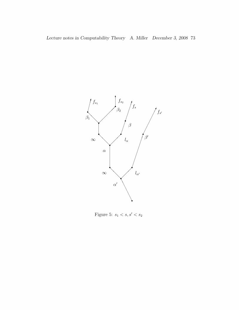
Lecture notes in Computability Theory A. Miller December 3, 2008 73
AA
AA
AA
@@
@
r
rα′
r r∞ lα′
rβ′
fs′
r
@@
@r r
r@@@
r6fs2β2
α
∞ lα
rβ
fsr fs1
β1
Figure 5: s1 < s, s′ < s2

Lecture notes in Computability Theory A. Miller December 3, 2008 74
QED
Exercise 32.2. Put the Friedberg-Muchnik argument on a tree of outcomes.Show there is no injury on the true path.
Exercise 32.3. Put the low simple non-auto-reducible set constructionon a tree of outcomes. Prove the construction works. Show that there is noinjury on the true path.
Exercise 32.4. (From Cooper) Show that there is minimal pair A0 and A1
such that (A0 ⊕ A1)′ ≡T 0′.
33 Friedberg: A one-one enumeration of the
c.e. sets
Theorem 33.1 (Friedberg, Enumeration without repetition) There exists ac.e. set U such that
1. Ue : e ∈ ω is the set of all c.e. sets and
2. Ue1 6= Ue2 for all e1 6= e2
ProofWe will first construct a c.e. set V and then modify it to get U . The
requirements are:Re ∀e < e (We 6= We)→ We = Vx for some unique x.
The strategy for meeting this requirement is to appoint a follower x. Aslong as it looks like ∀e < e (Wex 6= Wex) keep enumerating We into Vx.Otherwise make it a disloyal follower and put it into the garbage. Whatdo we do with Vx when x is a disloyal follower? We make it into an initialsegment.
Definition 33.2 A ⊆ ω is an initial segment iff A = ∅ or A = ω or thereexists n < ω such that A = [0, n] =def i < ω : 0 ≤ i ≤ n.

Lecture notes in Computability Theory A. Miller December 3, 2008 75
So our modified requirement is:
Re If ∀e < e (We 6= We) and We is not an initial segment, thenWe = Vx for some unique x.
At stage s+ 1 in our construction we have the following sets:
1. Fs the followers
2. a 1-1 mapping from Fs to ω which tells us that x is the follower of e,say fs(x) = e
3. Ds the disloyal former followers
4. (Vx,s : x ∈ Fs ∪Ds)
5. a nondecreasing variable gs keeping track of last initial segment assignedto a disloyal follower.
The sets Fs and Ds will be disjoint finite sets whose union is an initialsegment.
Construction
Stage s+ 1Let s = 〈e, ?〉. (So we visit each e infinitely often.)If no follower is assigned to Re, let x = min(Fs ∪Ds) and assign x to be
the follower of Re. Put Fs+1 = Fs ∪ x and end the stage.If x is the follower of Re and
1. ∀e < eWe,s+1 ∩ [0.x] 6= (We,s+1) ∩ [0, x]
2. We,s+1 ∩ [0, x] is not an initial segment
then put Vx,s+1 = Vx,s ∪ We,s+1 and end the stage. Actually in this caseVx,s ⊆ We,s so we could have said put Vx,s+1 = We,s+1.
If x is the follower of Re and either of those two conditions fails then
1. change x into a disloyal follower, i.e., Fs+1 = Fs \ x and Ds+1 =Ds ∪ x,

Lecture notes in Computability Theory A. Miller December 3, 2008 76
2. let gs+1 be the minimum g > gs such that Ve,s ⊆ [0, g], and
3. permanently assign Vx to be [0, gs+1], i.e., set Vx,s+1 = [0, gs+1] andnever change Vx again.
End the stage.
Verification
Claim 1. The following are equivalent for any e:
1. We is not an initial segment of ω and We 6= We for each e < e.
2. Re obtains a permanent follower x and hence Vx = We.
ProofSuppose condition 2 holds. Then Re obtains a permanent follower x. Thenfor all stages s+1 after x is appointed and for which s = 〈e, ?〉, we have thatWe,s ∩ [0, x] is not an initial segment and We,s ∩ [0, x] 6= We,s ∩ [0, x] for eache < e. Condition (1) follows since there are infinitely many such stages.
Suppose that condition 1 holds. Choose y so that We ∩ [0, y] is not aninitial segment and
We ∩ [0, y] 6= We ∩ [0, y]
for every e < e. Go to some stage s0 where
We,s0 ∩ [0, y] = We ∩ [0, y]
andWe,s0 ∩ [0, y] = We ∩ [0, y]
for every e < e. IfRe has no permanent follower then infinitely many followersare appointed to it. Hence some follower x > y will be appointed after stages0. But such a follower will always remain loyal.QED
Let D = ∪s∈ωDs be the set of disloyal followers. Then D is the set ofpermanent followers.
Claim 2.

Lecture notes in Computability Theory A. Miller December 3, 2008 77
1. Vx : x ∈ D is the set of c.e. sets which are not initial segments.
2. There exist a computable set G such that
[0, n] : n ∈ G = Vx : x ∈ D.
3. Vx 6= Vx′ unless x = x′.
ProofPart (1) follows from Claim 1.For Part (2), since the sequence gs is non-decreasing we see that
G = gs : s ∈ ω
is computable.For Part (3) note that there are two types of Vx. If x is a permanent
follower of some Re and then Vx = We where We is not an initial segmentand We is distinct from each We. Or x is a disloyal follower at some stages+ 1 and then Vx = [0, gs+1]. Since the sequence gs is bumped up each timeit is used we see that the Vx for disloyal followers are distinct finite initialsegments. This proves Claim.QED
Let us show how to modify V to U to prove Friedberg’s enumerationwithout repetition theorem. Note that V uniquely enumerates every c.e. setexcept ω, ∅, and the finite initial segments of the form [0, n] where n /∈ G.Let xn : 1 < n < ω be a 1-1 computable enumeration of G. Now define Uby U0 = ω, U2 = ∅, U2n = [0, xn] for n > 1, and U2n+1 = Vn.QED
Definition 33.3 A family of subsets V of ω is called a c.e. class iff thereexists a c.e. set V such that
V = Ve : e ∈ ω
where Ve = x : 〈e, x〉 ∈ V . V is call an enumeration of V. If Ve 6= Ve′whenever e 6= e′ then V is called a Friedberg enumeration of V.
Theorem 33.4 If V is a c.e. class containing all initial segments, then Vhas a Friedberg enumeration.

Lecture notes in Computability Theory A. Miller December 3, 2008 78
ProofThis is an obvious modification of the proof of Theorem 33.1.QED
Example 33.5 (Pour-El, Putnam) There is a c.e. class consisting of in-finitely many one and two element sets which has no Friedberg enumeration.
ProofTake A to be any set which is c.e. but not computable. Let Fn = 2n, 2n+1and Gn = 2n. Then
V = Fn : n ∈ ω ∪ Gn : n ∈ A
is a c.e. class. This is because we just enumerate 2n + 1 into Gn turningit into Fn when n is enumerated into A). But V cannot have a Friedbergenumeration V since then:
∀n (n ∈ A iff ∃x, y x 6= y and 2n ∈ (Vx ∩ Vy)).
QED
Example 33.6 (Pour-El, Putnam) There is an infinite c.e. class V con-taining ω such that any enumeration of V must list ω infinitely many times.
ProofLet A be any c.e. set which is not computable. Let V be the class of c.e. setsB such that B ⊆ A or B = ω. To see that V is a c.e. class just enumerateeach We into Ve as long as you see that As ∩ We,s = ∅. If this ever fails,enumerate all of ω into Ve.
If there is an enumeration of V which only lists ω finitely many times,then there is an enumeration U of the elements of V which are not ω. Butthen
A =⋃Ue : e ∈ ω
would the be a c.e. set.QED
It seems to require a more complicated proof than that for Theorem 40.6to show:
Theorem 33.7 (Friedberg) The class of graphs of partial computable func-tion has a Friedberg enumeration.
Lecture notes in Computability Theory A. Miller December 3, 2008 79
Exercise 33.8. Prove that the family of computable sets is a c.e. class andhas a Friedberg enumeration.
Exercise 33.9. Prove that the family of c.e. sets which are not simple is ac.e. class and has a Friedberg enumeration.
34 Hypersimple sets
Definition 34.1 Coding finite sets. For D ⊆ ω let x =∑
n∈D 2n. WriteDx = D.
Definition 34.2 (Dx : x ∈ R) is a strong array iff R is an infinite com-putable set and for every x, y ∈ R we have Dx ∩Dy = ∅ whenever x 6= y.
Definition 34.3 A set A ⊆ ω is hypersimple iff A is c.e. , A is infinite, andfor every strong array (Dx : x ∈ R) there exists x ∈ R such that Dx ⊆ A.
Proposition 34.4 (Post)(1) Hypersimple implies simple.(2) There is a simple set which is not hypersimple.(3) There is a hypersimple set.
Proof(1) If A is not simple, then there exists an infinite computable set R ⊆ A.Then D2x : x ∈ R witnesses that A is not hypersimple.(2) In Post’s original construction of a simple set A (see Theorem 15.2) weconstructed a simple set A by waiting until there was some x ∈ We,s withx > 2e and We,s ∩As = ∅ and then putting x into A. The reason that A wasinfinite was because for every e we had that |[0, 2e] ∩ A| ≤ e. This meansthat for every a we have that
[a, 4a] ∩ A 6= ∅
because [a, 4a] is 3/4 of the interval [0, 4a]. So define a0 = 5 and an+1 =4an + 1. Take xn so that Dxn = [an, 4an] and note that Dxn ∩ A 6= ∅ foreach n so the computable set R = xn : n < ω witnesses that A is nothypersimple.(3) This is a consequence of the following proposition, although originallyPost gave a construction similar to his construction of a simple set.QED

Lecture notes in Computability Theory A. Miller December 3, 2008 80
Proposition 34.5 (Dekker) Deficiency sets are hypersimple.
ProofSee Theorem 17.1. Suppose that A = as : s ∈ ω is a 1-1 computableenumeration of A and A is not computable. Define
D = s : ∃t > s at < as.
As we saw before A ≡T D and D is simple. A similar proof will show thatD is hypersimple.
Suppose for contradiction that there exists a strong array (Dx : x ∈ R)such that Dx ∩D 6= ∅ for every x ∈ R.
Now we get a contradiction by showing that A is computable.Input u. Find an x ∈ R such that
u < minas : s ∈ Dx.
Such an x exists, since as is a 1-1 enumeration and the Dx are pairwisedisjoint. But now at least one of t ∈ Dx is not deficient, so for all s > t wehave as > at. Hence u ∈ A iff u = as for some s ≤ maxDx.QED
Exercise 34.6. Define A to be bdd-hypersimple iff A is c.e. , A is infinite,and for every strong array (Dx : x ∈ R) such that there exists N < ω suchthat |Dx| ≤ N for all x ∈ R, there exists x ∈ R such that Dx ⊆ A. Provethat bdd-hypersimple is equivalent to simple.
Definition 34.7 For any set A ⊆ ω such that A is infinite define an to bethe (n+ 1)th element of A, i.e.,
A = a0 < a1 < · · · < an < · · ·.
Proposition 34.8 For any c.e. set A with A infinite the following are equiv-alent:
1. A is hypersimple.
2. For any computable increasing sequence nk < nk+1 there are infinitelymany k with [nk, nk+1) ⊆ A.

Lecture notes in Computability Theory A. Miller December 3, 2008 81
3. For any computable f ∈ ωω there are infinitely many k such that f(k) <ak.
Proof(1)→ (2). This is clear since if Dxk
= [nk, nk+1), then R = xk : k < ωis a strong array. There are infinitely many since R(l) =def xk : k > l is astrong array for any l.
(2) → (3). Given a computable f construct a computable sequencenk+1 > nk with the property that f(nk+1) < nk+1 for each k. For any k suchthat [nk, nk+1) ⊆ A note that A∩ [0, nk+1) ⊆ [0, nk) and so ank+1 = (nk+1)th
element of A must be greater than nk+1. Hence f(nk + 1) < ank+1.(3)→ (1). Suppose A is not hypersimple and hence there exists a strong
array (Dx : x ∈ R) such that Dx ∩ A 6= ∅ for all x ∈ A. Let xn : n ∈ ω)be a 1-1 computable enumeration of R and define
f(n) = 1 + max(∪m≤nDxm)
Then |A ∩ [0, f(n))| > n and so f(n) > an.QED
Exercise 34.9 Suppose A is hypersimple and f : ω → ω is computable.Prove there exist an infinite computable set C such that f(n) < an for alln ∈ C.
Exercise 34.10. Prove that for every c.e. set A ⊆ ω if A is infinite, thenthere exists a hypersimple set B ⊇ A.
Consider propositional logic with the set of atomic letters
Pn : n ∈ ω.
For any propositional sentence ψ and subset A ⊆ ω define
A |= ψ
inductively byA |= Pn iff n ∈ A
A |= ¬ψ iff not A |= ψ

Lecture notes in Computability Theory A. Miller December 3, 2008 82
A |= (ψ ∨ θ) iff (A |= ψ or A |= θ)
and so forth for the other logical symbols.By coding symbols as elements of ω and thinking of sentences as strings
of symbols or finite sequences of elements of ω, we identify the set of propo-sitional sentences with a computable subset of ω, SENT. The details of thiscoding are left to the reader.
The following notion is known as truth-table (tt) reducibility.
Definition 34.11 A ≤tt B iff there exists a computable sequence
(θn ∈ SENT : n ∈ ω)
such that for all n ∈ ωn ∈ A iff B |= θn
Note: It is easy to see that A ≤tt C and B ≤tt C implies (A ∩ B) ≤tt Cand A ≤tt C. Hence the family of sets which are truth-table reducible to C isclosed under finite boolean combinations. It is easy to see that ≤m-reducibleis stronger than ≤tt, and ≤tt is stronger than ≤T .
Proposition 34.12 (Nerode) The following are equivalent:
1. A ≤tt B.
2. There exist e with the property that
∀X ∀x eX(x) ↓
and eB = A.
3. There exists e and f ∈ ωω computable such that
∀x eBf(x)(x) ↓
and eB = A.
Proof(1) → (2). Given (θn : n ∈ ω) witnessing that A ≤tt B, it is easy to
construct an oracle machine e such that for any input x and oracle X thateX(x) ↓= 1, if X |= θx and eX(x) ↓= 0, if X |= ¬θx.

Lecture notes in Computability Theory A. Miller December 3, 2008 83
(2)→ (3). We show that the same e works. Input x and let
Tx = σ ∈ 2<ω : eσ|σ|(x) ↑.
The trees Tx are uniformly computable in x. By Konig’s tree lemma, sinceTx has no infinite branch, it is finite. Therefore we can compute the least nsuch that for all σ ∈ 2n we have that σ /∈ Tx. Put f(x) = n.
(3) → (1). Input x. Compute a use bound ux so that for every possiblecomputation e?f(x)(x) the computation only asks about i < ux. (Since it
takes at least one step to ask the oracle anything there are at most 2f(x) suchsimulations.)
Now definetx = R ⊆ [0, ux] : eRf(x)(x) ↓= 1.
Defineθx = ∨∨R∈tx(∧∧i∈R Pi ∧ ∧∧i∈[0,ux]\R ¬Pi)
Then for any x ∈ ω we have that
x ∈ A iff eBf(x)(x) ↓= 1 iff B ∩ [0, ux] = R ∈ tx iff B |= θx.
QED
Proposition 34.13 (Post)
1. If A is simple, then A <m K.
2. If A is hypersimple, then A <tt K.
3. There exists a simple A with A ≡tt K.
Proof(1) If K ≤m A then A is creative and hence not simple. (See Theorem
14.3.)(2) Since every c.e. set is many-one reducible to K it is enough to see
that K ≤tt A implies A is not hypersimple.
Claim. Let Γ = Pn : n ∈ A. Then there exists a computable list (ρn : n <ω) of propositional sentences such that for every n
1. A |= ρn and

Lecture notes in Computability Theory A. Miller December 3, 2008 84
2. Γ ∪ ρm : m < n 6` ρn.
ProofSince K ≤tt A there exists a computable function θ : ω → SENT such thatn ∈ K iff A |= θ(n).
Now we effectively construct ρn as follows. Let
Σn = ρ : Γ ∪ ρm : m < n ` ρ.
Note that Σn is computably enumerable as a subset of SENT. Also A |= θfor every θ ∈ Σn. It follows that θ−1(Σn) ⊆ K is c.e. By the S-n-m Theoremthere exists a computable function f such that
Wf(n) = θ−1(Σn)
and by the proof that K is creative we have that
f(n) ∈ K ∪ θ−1(Σn).
Take ρn = θ(f(n)).QED
Let Sk be that set of all n such that the propositional letter Pn occurs inthe sentence ρk, i.e., Sk is the support of ρk.
Claim. For any n let
m = max(⋃Sk : k ≤ 22n+1
+ 1)
then A ∩ [n,m) 6= ∅.ProofSuppose not and assume that [n,m) ⊆ A. Let ρ∗k be obtained from ρk byreplacing all propositional letters Pi for n < i < m by the letter Pn. Notethat Γ ` Pi for all these i and hence Γ ` ρ∗k ≡ ρk for every k ≤ 22n+1
+1. Butthere are at most 22n+1
logically inequivalent propositional sentences withatomic letters Pi for i ≤ n and so for some k < l we have that ρ∗k ≡ ρ∗l . Butthis is a contradiction since then
Γ ` ρi ≡ ρj.
QED

Lecture notes in Computability Theory A. Miller December 3, 2008 85
Now it is an easy matter to construct a computable sequence nk < nk+1
so that A ∩ [nk, nk+1) 6= ∅ for each k. Hence A is not hypersimple.
(3) Let B be any simple set which is not hypersimple. By Proposition34.8 there exists a computable increasing sequence (nk : k < ω) such that forall k we have that B ∩ [nk, nk+1) 6= ∅. Now let
A = B ∪⋃k∈K
[nk, nk+1)
A is simple because it is a superset of the simple set B. A is infinite becausefor each k ∈ K we have A ∩ [nk, nk+1) 6= ∅. We have that K ≤tt A because
k ∈ K iff A |= ∧∧nk≤i<nk+1Pi
QED
Exercise 34.14. Prove that ≤tt is transitive, i.e., A ≤tt B and B ≤tt Cimplies A ≤tt C.
35 Hyperhypersimple sets
Definition 35.1 V is a weak array iff V is c.e. and Vx ∩ Vy = ∅ wheneverx 6= y. As usual, Vx = y : 〈x, y〉 ∈ V .
Definition 35.2 A ⊆ ω is hyperhypersimple iff A is re, A is infinite, andfor every weak array V there exists x with Vx ⊆ A.
Proposition 35.3 For any A ⊆ ω for which A is c.e. and A is infinite thefollowing are equivalent:
1. A is hyperhypersimple
2. for every infinite c.e. set B such that Wx ∩ Wy = ∅ for all distinctx, y ∈ B there exists x ∈ B with Wx ⊆ A
3. for every weak array V there exists an infinite computable set R suchthat Vx ⊆ A for all x ∈ R
4. for every weak array V such that Vx is finite for all x there exists xsuch that Vx ⊆ A

Lecture notes in Computability Theory A. Miller December 3, 2008 86
Proof(1) iff (2) is true because the two types of arrays are the same.(1)→ (3), The sequence (Rn = 〈n,m〉 : m ∈ ω : n < ω) is a uniformly
computable partition of ω into infinite pieces. Take
Un = ∪e∈RnVe
Then U is weak array and so there exists n with Un ⊆ A.(4) → (1). Given a weak array V such that Ve ∩ A 6= ∅ for all e we find
another weak array V ∗ such that V ∗e finite and V ∗
e ∩A 6= ∅ for all e. For eachs define V ∗
e,s = Ve,s0+1 where s0 is the largest t ≤ s such that Ve,t ⊆ As.QED
Exercise 35.4. Prove(a) If A is simple and B is simple, then A ∩B is simple.(b) If A is hypersimple and B is hypersimple, then A∩B is hypersimple.(b) If A is hyperhypersimple and B is hyperhypersimple, then A ∩ B is
hyperhypersimple.
Example 35.5 There exists a hypersimple set A which is not hyperhyper-simple.
ProofLet B ⊆ ω be any hypersimple set. Define A ⊆ ω by
A = 〈n,m〉 : n ∈ B or n ≤ m.
See Figure 6. A is not hyperhypersimple since each of the horizontal lines:
Vk =def 〈m, k〉 : m ∈ ω
meets A. To see that A is hypersimple suppose we are given a strong array(Dn : n ∈ R). Let π(〈m,n〉) = m be projection to the first coordinate.We can find an infinite computable subset S ⊆ R such that (π(Dx ∩ Q) :x ∈ S) are pairwise disjoint where Q = 〈n,m〉 : m < n < ω. Since B ishypersimple, there exists x ∈ S with π(Dx ∩Q) ⊆ B and hence Dx ⊆ A.QED
Example 35.6 Dekker deficiency sets are never hyperhypersimple.

Lecture notes in Computability Theory A. Miller December 3, 2008 87
-
6
n ∈ B
&%'$Dx
"!# Dy
Vk
Figure 6: A = 〈n,m〉 : n ∈ B or n ≤ m.
ProofLet A = as : s ∈ ω be a one-one computable enumeration of a non com-putable set A. And D = s : ∃t > s at < as. We construct a weak array Vto meet the requirements:
Rx Vx ∩D 6= ∅
Stage s+1Step (a). For any x ≤ s if Rx has a follower t such that as < at then
unappoint t so that now Rx has no follower.Step(b). For the least x for which Rx has no follower, appoint s the
follower of Rx and put Vx,s+1 = Vx,s ∪ s.This ends the stage and the construction. Note that V is a weak array.
Claim. Each Rx obtains a permanent follower s and for this s we haves ∈ Vx ∩D.ProofThis is by induction on x. So after some sufficiently large stage s0 no y < xis appointed a new follower. Suppose for contradiction that Rx is appointeda new follower at stages s1, s2, . . . where s0 < s1 < s2 < · · ·. Note that sincehigher priority requirements don’t get new followers after s0 each time Rx

Lecture notes in Computability Theory A. Miller December 3, 2008 88
losses its follower it acquires the stage itself as its new follower. But thismeans that
as1 > as2 > as3 > · · ·
which is a contradiction.QED
Exercise 35.7. Prove that if A is hypersimple and (Dx : x ∈ C) is a strongarray then there exists an infinite computable E ⊆ C such that Dx ⊆ A forall x ∈ E.
36 Maximal sets
Definition 36.1 A ⊆∗ B iff B \ A is finite.A =∗ B iff A ⊆∗ B and B ⊆∗ A∀∞ means ‘for all but finitely many’∃∞ means ‘exists infinitely many’
Definition 36.2 M ⊆ ω is maximal iff M is c.e. , M is infinite, and forevery A c.e. if M ⊆ A then M =∗ A or A =∗ ω.
Proposition 36.3 Maximal sets are hyperhypersimple.
Suppose V is a weak array such that Ve ∩ A 6= ∅ for all e. Define
B = A ∪⋃e<ω
V2e
then A 6=∗ B and B 6=∗ ω, so A is not maximal.QED
Theorem 36.4 (Friedberg) Maximal sets exist.
ProofWe will construct the maximal set M as follows. We use the notation pn forthe nth element of the complement of M , i.e.,
M = p0 < p1 < p2 < · · ·
Are requirements are
Lecture notes in Computability Theory A. Miller December 3, 2008 89
Re (∀∞n pn ∈ We) or (∀∞n pn /∈ We)
This guarantees that M ∪We =∗ ω or M ∪We =∗ M ,At stage s given Ms we let
Ms = p0,s < p1,s < p2,s < · · ·
The idea of this proof is called moving markers. We think of a markerlabeled n with position pn,s. As we slide the marker upward we put theuncovered numbers into Ms. In order to get M infinite we want each markerto eventually stop moving.
Definition 36.5 σ ∈ 2n is the n-state of x at stage s iff
for all e < n σ(e) =
1 if x ∈ We,s
0 if x /∈ We,s
Two easy facts about the n-state are the following:
(1) Suppose s1 ≤ s2,σ1 ∈ 2n is the n-state of x at stage s1, andσ2 ∈ 2n is the n-state of x at stage s2,
then σ1 ≤lex σ2.
(2) For fixed n and x there is σ ∈ 2n such that σ is the n-state of x forall but finitely many stages s. We call this the final n-state of x.
Our strategy can be summarized simply as ‘maximize the lexicographicorder of the n-state of pn’.
Stage s+ 1.Find the least n (if any) such that there exists m with n < m < s such that
if σ ∈ 2n is the n state of pn,s andτ ∈ 2n is the n state of pm,s, then σ <lex τ .
For the least such n find the least m and shift the marker n to m:Put pn+i,s+1 = pm+i,s for all i < ω. Equivalently put
Ms+1 = Ms ∪ pj,s : n ≤ j < m
Otherwise as usual if there are no such n,m just go to the next stage witheverything unchanged.

Lecture notes in Computability Theory A. Miller December 3, 2008 90
This ends the stage and the construction.
Claim. The markers eventually stop moving, i.e.,
lims→∞
pn,s = pn <∞
ProofThis is proved by induction on n. Note that the only way the marker n movesis either that it is bumped up by some marker m < n or it moves to a highern-state. So consider some stage s0 so that no marker m < n moves afterstage s0. But it is impossible for pn to change infinitely many times afterthis since its n-state would have to increase lexicographically infinitely manytimes. (Note that in between moves its n-state might also change withoutthe marker moving but it can only increase if it doesn’t move.)QED
Claim. For each n there exists τ ∈ 2n such that
∀∞m τ = the final n-state of pm.
ProofSuppose not. Then there exists distinct τ1, τ2 ∈ 2n such that∃∞m τ1 = the final n-state of pm and∃∞m τ2 = the final n-state of pm.
Suppose τ1 <lex τ2. Then we can choose m1,m2 with n < m1 < m2 and thefinal n-state of pmi
is τi. This is a contradiction, since for some large enoughstage s0 > m2 the markers pj for j ≤ m2 have stopped moving and their finaln-states are their states at stage s0. But by the construction some marker≤ pm1 must move.QED
This final claim proves the Theorem, since if n = e+ 1 we have thatτ(e) = 1 implies ∀∞m pm ∈ We
andτ(e) = 0 implies ∀∞m pm /∈ We
QED
Example 36.6 There exists a hyperhypersimple set which is not maximal.

Lecture notes in Computability Theory A. Miller December 3, 2008 91
ProofFirst we note that it easy to get M1 and M2 maximal so that M1 6=∗ M2.Take any maximal set M and let R ⊆M to be an infinite computable subset.Let π : ω → ω be a computable bijection which takes R to R. Let M1 = Mand let M2 = π(M1).
Now let A = M1 ∩M2. Then A is hyperhypersimple (see exercise) butnot maximal since A ⊆M1 ⊆ ω and A 6=∗ M1 and M1 6=∗ ω.QED
Remark. Yates noted that we can add to the maximal set constructionan extra ‘kick’ to the pe marker to ensure that e(e) ↓ iff epe(e). Thenthe maximal set constructed will be Turing equivalent to K.
Exercise 36.7. Suppose A = an : n < ω is a 1-1 computable enumera-tion of a hyperhypersimple set A. Let B = aan : n < ω. Prove that B ishyperhypersimple but not maximal.
Exercise 36.8. A c.e. set A ⊆ ω is simple in R where R is an infinitecomputable set iff A ∩ R is infinite but contains no infinite c.e. subset. Isevery c.e. set which is not computable, simple in some infinite computableset? Hint: Split a maximal set.
37 The lattice of c.e. sets
Definition 37.1 The lattice of c.e. sets is E = (c.e.sets,⊆). A subsetX ⊆ E is definable iff there is a first order formula θ(v) in the language of⊆ such that
X = A ∈ E : E |= θ(A).
Similarly for X ⊆ E2 or X ⊆ E3.
Example 37.2 The following are definable in E.
1. (A,B,C) ∈ E3 : A ∪B = C
2. (A,B,C) ∈ E3 : A ∩B = C
3. ∅
4. ω

Lecture notes in Computability Theory A. Miller December 3, 2008 92
5. computable sets
A is computable iff E |= ∃B B ∩ A = ∅ and B ∪ A = ω
6. c.e. but not computable sets
7. infinite c.e. sets
A is infinite c.e. iff E |= ∃B B ⊆ A and B is not computable
8. finite sets
9. cofinite sets
10. ⊆∗, =∗
11. simple sets
12. maximal sets
Definition 37.3 π is an automorphism of E iff π : E → E is a bijectionsuch that for every A,B ∈ E
A ⊆ B iff π(A) ⊆ π(B).
Note that for any first-order formula θ(v1, . . . , vn) in the language of E ,i.e., ⊆, that for any π ∈ aut(E) and A1, . . . , An ∈ E we have that
E |= θ(A1, . . . , An) iff E |= θ(π(A1), . . . , π(An))
Hence definable sets are closed under automorphisms.
Example 37.4 If A ∈ E, then A is definable in E iff A = ∅ or A = ω.
ProofIf A is neither ∅ or ω, then we can choose n,m < ω such that n ∈ A andm /∈ A. Let π : ω → ω be the identity except π(n) = m and π(m) = n.Define π : P (ω) → P (ω) by π(A) = π(n) : n ∈ A. Then since π iscomputable it is clear that π ∈ aut(E). But since
π(A) = (A \ n) ∪ m
we see that A is not closed under automorphisms and hence cannot bedefinable.QED

Lecture notes in Computability Theory A. Miller December 3, 2008 93
Proposition 37.5 1. For every π ∈ aut(E) there exists a bijection π ofω such that π(A) = π(n) : n ∈ A.
2. Not every bijection π : ω → ω induces an automorphism of E.
3. There are continuum many bijections π : ω → ω which induce anautomorphism of E.
Proof(1) It is easy to see that the set of singletons
n : n ∈ ω ⊆ E
is definable in E . Hence any automorphism π : E → E must permute thesingletons. Define π(n) so that π(n) = π(n). But now for every n ∈ ω
n ∈ A iff n ⊆ A iff π(n) ⊆ π(A) iff π(n) ∈ π(A)
Hence π(A) = π(n) : n ∈ A.(2) Take any bijection which maps the even integers to some non com-
putable infinite coinfinite set.(3) Let M be a maximal set. Let π : ω → ω be any bijection such
that πM = id. There are continuum many such bijections, one for eachpermutation of M . But for any A ∈ E we have that A ∩ M is finite orA ∩M =∗ M . But this gives us that π(A) =∗ A. Similarly π−1(A) =∗ A.QED
The following theorem shows that the family of hyperhypersimple sets isdefinable in E .
Theorem 37.6 (Lachlan) A is hyperhypersimple iff A is c.e. , A is infinite,and
E |= ∀B ⊇ A ∃C ⊇ A B ∩ C = A and B ∪ C = ω
ProofSuppose A is not hyperhypersimple and V is a weak array such that Ve∩A 6= ∅for all e. Define
B = A ∪⋃e∈ω
(Ve ∩We)
Suppose for contradiction that C satisfies B ∩C = A and B ∪C = ω. Thenfor some e we have that C = We. Let x ∈ Ve ∩A. If x ∈ We then x ∈ C ∩B

Lecture notes in Computability Theory A. Miller December 3, 2008 94
but this contradicts B ∩ C = A. If x /∈ We then x /∈ C and x /∈ B but thiscontradicts B ∪ C = ω.
Conversely suppose there exists B as above for which there is no C.We must show there is a weak array V such that Ve ∩ A 6= ∅ for all e.So let B = bs : s ∈ ω be a 1-1 computable enumeration of B and putBs = bt : t < s. Similarly, let As be a computable enumeration of A.
We will construct Ve,s pairwise disjoint subsets of B and meet the require-ments:
Re Ve ∩ A 6= ∅
We will carry along g(e, s) a gate which we use to let elements into eachVe. At stage s = 0 as usual we put Ve,s = ∅ and g(e, s) = 0.
Construction
Stage s+ 1.First define g(e, s + 1) for e < s. If Ve,s ⊆ As, then g(e, s + 1) = g(e, s) + 1.In other words, if the requirement Re is not looking good, then incrementthe gate, otherwise let it alone.
Look for the least e < s (if any) such that bs ≤ g(e, s+1) and put bs intoVe, i.e.,
Ve,s+1 = Ve,s ∪ bs.
If there is no such e, do nothing. This ends the construction.
Verification
Claim. lims→∞ g(e, s) = g(e) <∞ and Re is met.ProofThis is proved by induction on e. Choose s0 so that for all e < e and s > s0
we have that g(e, s) = g(e) and
bs > maxg(e) : e < e
Suppose for contradiction that
lims→∞
g(e, s) =∞

Lecture notes in Computability Theory A. Miller December 3, 2008 95
DefineC = A ∪
⋃s≥s0
([0, g(e, s+ 1)] ∩Bs
Suppose x ∈ A. Then we claim that
x ∈ C iff x ∈ B
This is a contradiction since then C ∩B = A and C ∪B = ω.Suppose x ∈ B. This implies that x ∈ Bs for all s. But if g(e, s) → ∞
we have that x ∈ C.Suppose x ∈ C. Then for some s ≥ s0 we have that x ∈ [0, g(e, s)] ∩ Bs
(since we are assuming x /∈ A.) If x /∈ B then x ∈ B \ Bs. Hence x = bt forsome t ≥ s. But notice that bt = x ≤ g(e, s) ≤ g(e, t + 1). By our choiceof s0 we have that bt > g(e) for all e < e and so bt will be put into Ve. Butx = bt was assumed to be an element of A. This means that g(e, t) will neverincrease again which contradicts it going to ∞.
The reason Re is met is because if g(e, s) stops growing then eventuallywe stop putting bs’s into Ve. Hence Ve is finite and so it is impossible thatVe ⊆ A.
This proves the Claim and the Theorem.QED
The following shows that the family of hypersimple sets is not definablein E .
Theorem 37.7 (Martin) There exists a hypersimple set A and π ∈ aut(E)such that π(A) is not hypersimple.
ProofWe will construct the c.e. set A as usual by constructing a computableincreasing sequence As. We will construct a computable sequence πs of bi-jections of ω with the property that πs(n) = n for every n ≥ s. So each πs isreally a finite permutation. π will be the limit of πs.
Let W ∗e,s be defined as follows:
W ∗e,s = We,s0 where s0 ≤ s is the largest t ≤ s with the property that for
distinct x, y ∈ We,t we have that Dx ∩Dy = ∅.The list W ∗
e automatically contains all strong arrays. Our requirementsfor this construction include:
Re W ∗e infinite → ∃x ∈ W ∗
e Dx ⊆ A

Lecture notes in Computability Theory A. Miller December 3, 2008 96
The strategy for making sure that A is a variant on the Post 2e strategy.At stage s = 0 in our construction we have As = ∅ and πs the identity.
Stage s+ 1.Given πs and As, we say that e < s requires attention iff
1. ¬∃n ∈ W ∗e,s Dn ⊆ As
2. ∃x, y such that
(a) x, y /∈ As(b) ∃n ∈ W ∗
e,s x ∈ Dn
(c) e < x < y < s, e < πs(x), e < πs(y)
(d) i. e-state of x at stage s = e-state of y at stage s
ii. e-state of πs(x) at stage s = e-state of πs(y) at stage s
(e) 2x < πs(y).
The action at this stage is the following. For the least e < s (if any) whichrequires attention we choose the least x for which there is a y and then wechoose the least y. For this choice (e, x, y) = (es, xs, ys) we
(a) put x into A, As+1 = As ∪ xs(b) put πs+1 = πsswap(x, y) where swap(x, y) refers to the transposition
which interchanges x and y.As usual if there is no e which requires attention we do nothing and go ontothe next stage.
This ends the construction. Let Q denote the stages s where action takesplace at stage s+ 1. Then
A = xs : s ∈ Q
We defineπ(u) = lim
s→∞πs(u)
although at this point we have not proved that this limit always exists. Notethe pointwise limit of 1-1 functions must be 1-1 where it is defined.
Note that for s ∈ Q we have that πs+1(xs) = πs(ys). Since xs entersA we have (by 2a) that xs will never be a xt or yt latter. It follows thatπ(xs) = πs+1(xs). Hence
B =def πs+1(xs) : s ∈ Q = π(xs) : s ∈ Q
Lecture notes in Computability Theory A. Miller December 3, 2008 97
is well defined and c.e.
Claim (1) for any n we have that |B ∩ [0, 2n]| ≤ n.ProofNote that (by 2e) we have that π(xs) = πs(ys) > 2xs. Since each xs is distinctthe Claim follows.QED
As we have seen before this implies that B is not hypersimple. (Proposi-tion 34.4).
Claim (2) lims→∞ πs(u) = π(u) <∞ for every u.ProofFix s0 so that A∩ [0, u] = As0∩ [0, u]. Now the only way that πs+1(u) 6= πs(u)for some s > s0 is if u = xs or u = ys. But in either case since xs < ys andxs enters A we have A changes in the interval [0, u] which is a contradiction.QED
We don’t know yet that π is onto.
Claim (3) For each e(a) Re is met.(b) ∃s0 ∀s > s0 es > e
ProofThis is proved by induction on e.
(a) We may suppose by induction that there exists s0 such that es ≥ e forall s > s0. Suppose Re is not met. Then W ∗
e is infinite and for all n ∈ W ∗e
we have that Dn ∩ A 6= ∅. For each n ∈ W ∗e define
un = min(Dn ∩ A)
Since the Dn are pairwise disjoint all of the un are distinct. Note there existσ, τ ∈ 2e such that∃∞n ∈ W ∗
e σ = final e-state of un and τ = final e-state of π(un).Choose un and um such that
1. n,m ∈ W ∗e
2. e < un < um
3. 2un < π(um)
Lecture notes in Computability Theory A. Miller December 3, 2008 98
4. σ is the final e-state of un and um, and
5. τ is the final e-state of π(un) and π(um).
Increase s0 (if necessary) so that not only is es ≥ e for all s ≥ s0 but alsoso that
1. n,m ∈ W ∗e,s0
2. un < um < s0 and π(un) < s0 and π(um) < s0
3. πs(un) = π(un) and πs(um) = π(um) all s > s0
4. σ is the e-state of un and um at stage s0,
5. τ is the e-state of π(un) and π(um) at stage s0 and
6. As0 ∩ [0, um] = A ∩ [0, um]
Recall that we chose un, um ∈ A. It is easy to check that e requiresattention at stage s0 and un and um witness this fact. But this means thatun or some smaller u enters A. But this contradicts the condition that Adoes not change below um.
(b) Suppose that es ≥ e for all s > s0 and Re is met. If W ∗e is infinite,
then for some n ∈ W ∗e we have that Dn ⊆ A. But this will be seen at some
stage and so e will not require attention after that. If W ∗e is finite, then
suppose that∪Dn : n ∈ W ∗
e ⊆ [0, N ].
After we reach a stage s > s0 where As ∩ [0, N ] = A ∩ [0, N ], then e willnever again require attention because then A would change beneath N .QED
Claim (4) π is onto.ProofGiven z choose s0 so that es > z for all s ≥ s0. If πs0(u) = z, then u willnever be either xs or ys for any s ≥ s0. This is because we required (2c) thatπs(xs), πs(ys) > es. Hence π(u) = z.QED
Claim (5)(a) ∀C ∈ E π(C) ∈ E
Lecture notes in Computability Theory A. Miller December 3, 2008 99
(b) ∀C ∈ E π−1(C) ∈ EProof
(a) Fix s0 so that for all s > s0 we have that es > e. Then we show that
π(We) =⋃s>s0
πs(We,s)
To see this first suppose y ∈ π(We). Then there exists x ∈ We with π(x) = ybut for all sufficiently large s we have that x ∈ We,s and πs(x) = π(x) andthus y ∈ πs(We,s).
To see the other inclusion, suppose that y ∈ πs(We,s) for some s > s0.We claim that for every t > s that y ∈ πt(We,t). This is proved by inductionon t. Suppose that πt(u) = y for some u ∈ We,t. Then πt+1(u) = πt(u) unlessu = xt or u = yt and then πt+1(xt) = πt(yt) and πt+1(yt) = πt(xt). But sincext and yt have the same et-state and et > e, if one is in We,t so is the other.In either case we have that there exists v ∈ We,t+1 with πt+1(v) = y. Nowto see that y ∈ π(We) suppose that π(u) = y and choose sufficiently larget > s0 such that πt(u) = π(u) = y. Since πt is a bijection and y ∈ πt(We,t),it must be that u ∈ We,t and hence u ∈ We.
(b) This is similar, except we use that πt(xt) and πt(yt) have the sameet-state.QED
Exercise 37.8. Prove that there exists a bijection π : ω → ω such thatπ(A) ∈ E for all A ∈ E but π /∈ aut(E). (Hint: use a maximal set.)
Exercise 37.9. For each n ≥ 2 prove there is a sequence of maximal setsA1, . . . , An such that Ai 6=∗ Aj for distinct i and j. Prove that for any suchsequence that E∗(A1∩A2∩· · ·∩An) is isomorphic to (P(1, . . . , n),⊆). Thestructure E∗(A) is the set of c.e. supersets of A modulo the finite sets andordered by ⊆∗.
38 Arithmetic hierarchy
Definition 38.1 For A and B predicates over subsets of ω or finite productsof ω we define:
Π00 = Σ0
0 = the computable predicates.A is Σ0
n+1 iff there exists B which is Π0n and A(x) ≡ ∃y B(x, y).

Lecture notes in Computability Theory A. Miller December 3, 2008 100
A is Π0n+1 iff there exists B which is Σ0
n and A(x) ≡ ∀y B(x, y).A is ∆0
n iff A is Σ0n and A is Π0
n.
Note that by DeMorgan’s Laws
Π0n = ¬A : A ∈ Σ0
n and Σ0n = ¬A : A ∈ Π0
n
and hence∆0n = ¬A : A ∈ ∆0
n.
Proposition 38.2 Suppose Γ is Σ0n, Π0
n, or ∆0n. Then Γ is closed under ≤m,
i.e., A ≤m B ∈ Γ implies A ∈ Γ. This implies that if the predicate B(x, y)is in Γ and f is a computable function, then A(x, y) ≡ B(x, f(x)) is in Γ.
Proposition 38.3 If B(x, y) in Σ0n, then A(x) ≡ ∃y B(x, y) is in Σ0
n. IfB(x, y) in Π0
n, then A(x) ≡ ∀y B(x, y) is in Π0n.
Proposition 38.4 Suppose Γ is Σ0n, Π0
n, or ∆0n. If A,B ∈ Γ, then A ∧
B and A ∨ B are both in Γ. Also, Γ predicates are closed under boundedquantification, e.g., ∃u < x A(u, x, . . .) and ∀u < x A(u, x, . . .).
Proposition 38.5 Σ0n ∪ Π0
n ⊆ ∆n+1 = Σ0n+1 ∩ Π0
n+1
Definition 38.6 We say that A is universal for Γ iff
Γ = Ax : x ∈ ω.
We say that A is m-complete for Γ iff
Γ = B : B ≤m A
Note that universal for Γ implies m-complete for Γ. Also, the complementof a set universal for Γ is universal for Γ and the same for m-completeness.
Proposition 38.7 For each n > 0 there is a universal Σ0n set.
Proposition 38.8 For each n > 0 we have Red(Σ0n), Sep(Π
0n), ¬Sep(Σ0
n),and ¬Red(Π0
n).

Lecture notes in Computability Theory A. Miller December 3, 2008 101
ProofSee definitions 8.2. We first show Red(Σ0
n). Let
A(x) ≡ ∃y R(x, y) and B(x) ≡ ∃y S(x, y)
where R and S are ∆0n. Reduce A and B by
A0(x) ≡ ∃y (R(x, y) ∧ ∀z < y ¬S(z, x))
andB0(x) ≡ ∃y (S(x, y) ∧ ∀z ≤ y ¬R(z, x))
Since Red(Γ)→ Sep(Γ) Proposition 8.4, it follows that Sep(Π0n) holds.
To see ¬Sep(Σ0n), first construct a doubly universal pair A and B. These
are Σ0n sets such that for every pair C and D of Σ0
n sets there exists a u withC = Au and D = Bu. To get A and B let U be a universal Σ0
n set. Thendefine
A = (〈x, y〉, z) : 〈x, z〉 ∈ U
andB = (〈x, y〉, z) : 〈y, z〉 ∈ U
then u = 〈x, y〉 codes the pair Ux and Uy. Now applying reduction to A andB we get A0 ⊆ A and B0 ⊆ B. Note that this simultaneously reduces allcross sections Au and Bu. Assuming for contradiction that separation holds,let C be ∆0
n such that A0 ⊆ C and B0 ⊆ C. We get a contradiction since,then C would be a universal ∆0
n set. This is because if P is ∆0n then there
exists u with Au = P and Bu = P . But the reduction followed by separationcan’t effect the u cross section, so Cu = P .QED
Exercise 38.9. Prove there does not exist a universal ∆0n set.
39 Post: ∆02 same as computable in 0′
Lemma 39.1 A ⊆ ω is Π02 iff there exists P computable such that
A(x) iff ∃∞s P (s, x)

Lecture notes in Computability Theory A. Miller December 3, 2008 102
Proof(←) ∃∞s P (s, x) iff ∀t ∃s > t P (s, x)(→) Suppose
A(x) iff ∀n ∃m R(n,m, x)
where R is ∆01. Define P ⊆ ω<ω × ω by
P (σ, x) iff ∀i < |σ| [R(i, σ(i), x) and ∀j < i ¬R(i, j, x)]
QED
Theorem 39.2 (Post) Suppose A ⊆ ω. Then A is ∆02 iff A ≤T 0′
ProofSuppose A is ∆0
2. Then by Lemma 39.1 there exists computable P (u, x) andQ(v, x) such that
A(x) ≡ ∃∞u P (u, x)
¬A(x) ≡ ∃∞v Q(v, x)
Now define g(x, s) as follows. Input x, s and let us be the maximum u ≤ ssuch that P (u, x) (zero if no such u). Similarly define vs to be the maximumv ≤ s such that Q(v, x). Define
g(x, s) =
1 if us ≥ vs0 if us < vs
It is easy to check thatA(x) = lim
s→∞g(x, s)
and so by the Limit Lemma 28.1 we have that A ≤T 0′.Conversely if A ≤T 0′ then by the Limit Lemma we have g computable
such thatA(x) = lim
s→∞g(x, s)
but thenA(x) ≡ ∀∞s g(x, s) = 1 ≡ ∃∞s g(x, s) = 1
so A is ∆02.
QED
Lemma 39.3 (1) A ⊆ ω is Σ01(B) iff A ≤m B′.
(2) A is ∆02(B) iff A ≤T B′.

Lecture notes in Computability Theory A. Miller December 3, 2008 103
ProofA is Σ0
1(B) iff there exists a predicate R ≤T B such that
A(x) iff ∃y R(x, y)
(1) is just a relativization of the standard result that 0′ is m-complete for Σ01.
(2) is just the relativization of Post’s Theorem 39.2.QED
Theorem 39.4 (Post)(1) A ≤T 0(n) iff A is ∆0
n+1.(2) 0(n) is an m-complete Σ0
n-set.
Proof(1) for n = 2:
A ≤T 0′′ iff A ≤T (0′)′ iff A is ∆02(0
′).A is ∆0
2(0′) iff there exists R1, R2 ≤T 0′ such that
A(x) iff ∃n ∀m R1(n,m)
¬A(x) iff ∃n ∀m R2(n,m)
but since R1, R2 ≤T 0′ iff R1 and R2 are ∆02, we have that
A is ∆02(0
′) iff A is ∆03.
(2) for n = 2:0′′ is Σ0
1(0′) and m-complete for Σ0
1(0′). But Σ0
1(0′) is Σ0
2. This is becauseB is Σ0
1(0′) iff there exists R ≤T 0′ such that
B(x) iff ∃y R(x, y)
But R ≤T 0′ iff R is ∆02. Hence B is Σ0
2 iff B is Σ01(0
′).
The proofs for n > 2 are analogous.QED
Exercise 39.5. Prove there does not exist A which is m-complete for ∆02.
Exercise 39.6. (Enderton, Putnam) Prove that if 0(n) ≤T A for every n,then 0(ω) ≤T A′′.Hint: Show that
P (e1, e2) ≡ ∃B,C B = e1A ∧ C = e2A ∧ C = B′
is Π02(A).

Lecture notes in Computability Theory A. Miller December 3, 2008 104
40 EMP, TOT, FIN, and REC
Proposition 40.1 EMP =def e : We = ∅ is Π01-m-complete.
Proofe ∈ EMP iff ∀x, s x /∈ We,s
so EMP is Π01. Let A be Π0
1, then there is R computable so that
A(x) iff ∀y R(x, y).
Using S-n-m Theorem get f computable so that for every x
Wf(x) = y : ¬R(x, y)
Then A(x) iff f(x) ∈ EMP .QED
Proposition 40.2 TOT =def e : We = ω is m-complete for Π02.
FIN =def e : We is finite is m-complete for Σ02.
Proofe ∈ TOT iff ∀x ∃s x ∈ We,s
e ∈ FIN iff ∃x ∀y, s (y ∈ We,s → y < x)
so TOT is Π02 and FIN is Σ0
2. Now suppose that A is Π02 we show that
(A,A) ≤m (TOT, FIN)
which simultaneously shows that TOT is Π02-m-complete and FIN is Σ0
2-m-complete. Suppose
A(x) iff ∃∞s P (s, x)
where P is ∆01. Using S-n-m find a computable function f so that
Wf(x) = t : ∃s > t P (s, x)
Hence A(x)→ Wf(x) = ω while ¬A(x)→ Wf(x) is finite.QED
Proposition 40.3 COF =def e : We is finite is Σ03-m-complete.

Lecture notes in Computability Theory A. Miller December 3, 2008 105
Proofe ∈ COF iff ∃n ∀m > n ∃s m ∈ We,s
Now suppose that A is Σ03. Then there exists P which is ∆0
1 such that
A(x) iff ∃n ∃∞m P (n,m, x)
Input x and describe the c.e. set Bx by using a moving marker constructionsimilar to the construction of a maximal set but simpler. At any stage s wehave that
Bx,s = p0,s < p1,s < p2,s < · · ·
We look for the least n < s (if any) such that P (n, s, x) and bump the nth
marker, i.e., enumerate pn,s into Bx, i.e., Bx,s+1 = Bx,s ∪ pn,s. Note that ifA(x) is true then there exist n so that the nth marker is bumped infinitelyoften and so Bx is cofinite. On the other hand if ¬A(x), then each markereventually stops moving and so Bx is coinfinite.
By the usual S-n-m argument we can find a computable function f sothat Bx = Wf(x) for all x and so
A(x) iff f(x) ∈ COF
QED
Proposition 40.4 REC =def e : We is computable is Σ03-m-complete.
Proofe ∈ REC iff ∃e′ (We ∪We′ = ω and We ∩We′ = ∅)
and We∪We′ = ω is Π02 and We∩We′ = ∅ is Π0
1. To see that it is m-complete,use a moving marker argument as above. Just add an additional reason tobump the eth marker to make sure that if Bx is coinfinite, then for each e
ψe(e) ↓ → ψe,pe(e) ↓
This guarantees that if Bx is coinfinite, then K ≤T Bx.QED
Exercise 40.5.(a) Let A be an infinite c.e. set. Let
QA = e : We = A

Lecture notes in Computability Theory A. Miller December 3, 2008 106
Prove that QA is Π02-m-complete.
(b) Let A be a finite nonempty set. Prove that
QA = e : We = A
is D(Σ01)-m-complete, where
D(Σ01) = A ∩B : A,B ∈ Σ0
1.
Lemma 40.6 Suppose A is Σ0k+1 then there exists B Π0
k such that
A(x) iff ∃y B(x, y) iff ∃!y B(x, y)
ProofSuppose
A(x) iff ∃y P (x, y)
where P is Π0k. Then
A(x) iff ∃y (P (x, y) ∧ ∀z < y ¬P (x, z)
DefineC(x, y) iff ∀z < y ¬P (x, z)
In case k+ 1 = 1 then C is ∆01. In case k+ 1 > 1 then since C is Σ0
k we haveby induction a Π0
k−1 predicate D so that
C(x, y) iff ∃u D(x, y, u) iff ∃!u D(x, y, u)
Hence
A(x) iff ∃y ∃u (P (x, y) ∧D(x, y, u)) iff ∃!y ∃!u (P (x, y) ∧D(x, y, u))
so taking B(x, 〈y, u〉) ≡ P (x, y) ∧D(x, y, u) does the trick.QED
Proposition 40.7 (a) A is Π03 iff there exists B which is ∆0
1 such that
A(u) ≡ ∃∞s ∀n B(s, n, u)
(b) A is Π04 iff there exists B which is ∆0
1 such that
A(x) ≡ ∃∞s ∃∞t B(s, t, x)

Lecture notes in Computability Theory A. Miller December 3, 2008 107
Proof(a) Suppose
A(u) ≡ ∀x ∃y ∀z R(x, y, z, u)
where R is ∆01. Define
Q(x, u) ≡ ∃y ∀z R(x, y, z, u)
Then by Lemma 40.6 there is a C which is Π01 and
Q(x, u) ≡ ∃y C(x, y, u) ≡ ∃!y C(x, y, u)
HenceA(u) ≡ ∀x∃!y C(x, y, u)
A(u) ≡ ∃∞σ ∈ ω<ω ∀i < |σ| C(i, σ(i), u)
Note that ∀i < |σ| C(i, σ(i), u) is Π01 and so there is B computable so that
∀n B(σ, n, u) ≡ ∀i < |σ| C(i, σ(i), u)
(b) SupposeA(u) ≡ ∀x ∃y R(x, y, u)
where R is Π02. By Lemma 40.6 applied to ∃y R(x, y, u) we may assume that
A(u) ≡ ∀x ∃!y R(x, y, u)
HenceA(u) ≡ ∃∞σ ∀i < |σ| R(i, σ(i), u)
but the predicateQ(σ, u) ≡ ∀i < |σ| R(i, σ(i), u)
is Π02 so there exists a computable B so that
Q(σ, u) ≡ ∃<∞τ B(σ, τ, u)
HenceA(u) ≡ ∃∞σ ∃∞τ B(σ, τ, u)
QED

Lecture notes in Computability Theory A. Miller December 3, 2008 108
Exercise 40.8. For the correct class Γ, show that INF, EQ, EQ* arem-complete Γ sets where
INF = e : We is infinite
EQ = 〈e1, e2〉 : We1 = We2
andEQ∗ = 〈e1, e2〉 : We1 =∗ We2.
Exercise 40.9.Let PTIME = e : ψe runs in polynomial time , i.e., there exists a
polynomial p(x) such that ψe(x) halts in less than p(x) steps for every x.Prove that PTIME is Σ0
2-m-complete.
Exercise 40.10. For each e let Qe = nm+1
: 〈n,m〉 ∈We ⊆ Q. DefineΩ = e : Qe is order isomorphic to ω.
Prove that Ω is Π03-m-complete.
Exercise 40.11. Show that if Q = e : We ∈ V is not Σ03 then V cannot
be a c.e. class. See Definition 33.3.
Exercise 40.12. Prove that the family of coinfinite c.e. sets is not a c.e.class.
Exercise 40.13. Prove that SIMP=e : We is simple is m-complete Π03.
Hint: Like the proof for COF but also let We kick the eth marker at mostonce to make A meet We if We infinite.
Exercise 40.14. Prove that the family of simple sets is not a c.e. class.
Exercise 40.15. Prove of disprove:(a) there exists a total f ≤T 0((2) such that for all e, if We is computable,
then Wf(e) = We.(b) there exists a total f ≤T 0(3) such that for all e, if We is computable,
then Wf(e) = We.
Lecture notes in Computability Theory A. Miller December 3, 2008 109
41 Domination and high degrees
Theorem 41.1 (Martin) For any set A ⊆ ω the following are equivalent:
1. 0′′ ≤T A′ and
2. there exists g ≤T A such that ∀∞n f(n) ≤ g(n) for every computablef .
Proof(1)→ (2)Since TOT is Turing equivalent to 0′′ (40.2), by the limit lemma (28.1)
there is a total h ≤T A so that for every e ∈ ω
T0T(e) = lims→∞
h(e, s).
Define he(x) = h(e, x) and define g(x) to be the maximum of the set:
e(x) : e < x and es(x) ↓ where he[x, s) ≡ 1.
Note that if e is not total, then he is eventually zero. If it is total thenhe is eventually one. It is easy to check that g ≤T h ≤T A and g eventuallydominates each computable functions.
(2)→ (1)Define
h(e, s) =
1 if eg(s)(x) ↓ for all x < s0 otherwise.
Then since g eventually dominates all computable functions we get that
T0T(e) = lims→∞
h(e, s)
and hence by the limit lemma that
0′′ ≡T T0T ≤T A′.
QED
Theorem 41.2 (Martin, Tennenbaum) If A is a maximal set, then
A′′ ≡T 0′′.

Lecture notes in Computability Theory A. Miller December 3, 2008 110
ProofLet g(n) = an where A = a0 < a1 < · · ·. We already know that sinceA is hypersimple that ∃∞n f(n) < g(n) for any computable f . Suppose∃∞n g(n) < f(n). Then there is a strong array 〈Fn : n < ω〉 such that|Fn ∩ A| ≥ 2 for infinitely many n. This because there must be infinitelymany n with
f(n) ≤ g(n) < g(n+ 1) < f(n+ 1)
and hence Fn = [f(n), f(n+1)) does the trick. But as in the characterizationof hyperhypersimple (35.3 part 4) there is a weak array 〈Hn ⊆ Fn : n < ω〉such that for every n if Fn ∩ A 6= ∅, then |Hn ∩ A| = 1. But then
A ⊆ A ∪⋃n
Hn ⊆ ω
shows that A is not maximal.QED
Theorem 41.2 is also true for the hyperhypersimple sets. Martin hasshown the converse that every high c.e. degree contains a maximal set.
Exercise 41.3. Prove that if for all f partial computable we have that
∀∞n ∈ dom(f) f(n) ≤ g(n)
then 0′ ≤T g.
Example 41.4 Suppose A is maximal and B = A ⊕ A. Then B is notmaximal, but 〈bn : n < ω〉 eventually dominates every computable function.
ProofIt is not maximal since B ⊆ (B ⊕ Evens) ⊆ ω and these inclusions are nontrivial.
To see domination note that b2n = 2an and b2n+1 = 2an + 1. For anycomputable f
∀∞n (f(2n), f(2n+ 1) < an < b2n < b2n+1)
and hence∀∞m f(m) < bm.
QED

Lecture notes in Computability Theory A. Miller December 3, 2008 111
Example 41.5 There is a c.e. set A which is not hyperhypersimple but aneventually dominates every computable function.
ProofLet Fk = [nk, nk+1) be the strong array with nk+1 = nk + k + 1. Note that|Fk| = k. Let B any maximal set. For each k and l if |B ∩ k| = l let Gk bethe top l elements of Fk. It is easy to see that 〈Gk ⊆ Fk : k ∈ ω〉 is a weakarray. Let
A =⋃
Gk ∪⋃k∈B
Fk.
Note that for every k|Fbk \Gbk
| = k.
For each l < ω define
Pl = nk + l : l < k < ω
then 〈Pl : l < ω〉 is a weak array demonstrating that A is not hyperhyper-simple. Note that
Fbk \Gbk= ai : lk ≤ i < lk+1
where lk+1 = lk + k and so lk = k(k+1)2
. Hence for any computable function fwe have that
∀∞k f(lk+1) < bk < alk
and so for f increasing we have:
∀∞m f(m) < am.
QED
Exercise 41.6. Prove that for any maximal set B
∀∞n f(bn) < bn+1
for every computable f .

Lecture notes in Computability Theory A. Miller December 3, 2008 112
42 High degrees using the Psuedojump
Theorem 42.1 (Shoenfield, Sacks) There is a nontrivial high degree, i.e.,there exists a c.e. set A with A <T 0′ and A′′ ≡T 0′′.
ProofThis was originally proved using an infinite injury priority argument. Wegive here a proof due to Jockusch and Shore which needs only a finite injurypriority argument together with relativization and uniformization.
Define that pseudojump operator Je as follows:
Je(A) = A⊕WAe .
Lemma 42.2 For any e0 there exists a c.e. set A withA >T 0 and Je0(A) ≡T 0′.
ProofLet 0′ = es : s < ω be a one-to-one computable enumeration of 0′ = K.
Requirements and strategies
Our requirements can be described as follows:
P2e A 6= We
Our strategy will be to put its follower v2e into A if it ever turns up in We.
P2e+1 Code e into A if e every turns up in 0′.
Our strategy will put its follower v2e+1 into As+1 if e = es. We will show thatv2e+1 can be computed from Je0(A) and so 0′ ≤T Je0(A).
Nn (∃∞s e0Ass (n) ↓)→ e0A(n) ↓
This is to insure that WAe0≤T 0′. We use the usual low simple set strategy
of restraining the computation.
Construction
For each negative requirement Nn define the restraint function r(n, s)to be the use of the computation e0As
s (n) (recall that this is zero if thecomputation does not converge).

Lecture notes in Computability Theory A. Miller December 3, 2008 113
For each positive requirement Pn its set of potential followers is
Fn = 〈n,m〉 : m < ω
and its follower vsn at stage s is:
vsn = minv ∈ Fn : v > max(r(m, s) : m ≤ n).
We say that Pn requires attention at stage s iff
1. (n = 2e+ 1 and e = es) or
2. n = 2e < s and W se ∩ As = ∅ and vsn ∈ W s
e .
Put As+1 = As ∪ vsn : Pn requires attention at stage s.
Verification
Note that each positive requirement can act at most once. It follows that
lims→∞
r(n, s) = r(n) <∞
and each Nn and Pn is met. Hence we have that WAe0≤T 0′ and A >T 0. It
remains only to see the following:
Claim. 0′ ≤T A⊕WAe0
.
Define
f(n) =
1 if Pn ever acts0 otherwise.
Obviously 0′ ≤T f since e ∈ 0′ iff f(2e+ 1) = 1. So it is enough to see that
f ≤T A⊕WAe0.
Assume we have computed fn using an oracle for A⊕WAe0
and we showhow to compute f(n). Find a stage s0 so that
1. ∀m < n if Pm ever acts, it has already acted by stage s0, and
2. ∀m ≤ n e0A(m) ↓ iff e0As0s0 (m) ↓.

Lecture notes in Computability Theory A. Miller December 3, 2008 114
Using the oracle (n ∈ WAe0
?) we can test that s0 satisfies (2), but since
r(m, s0) will protect the computation e0As0s0 (m), this will in fact be the
correct computation at all stages s ≥ s0. It follows that r(m, s) = r(m, s0)for all m ≤ n and s ≥ s0. Therefor v(n, s) = v(n, s0) for all s ≥ s0. Hence Pnwill act iff either it has already by stage s0 or v(n, s0) ∈ A (which happensiff it acts after s0).
This proves the Claim and the Lemma.QED
Next we need to see that a relativized and uniformitized version of theLemma is true.The Lemma says:
For all e there exists a c.e. set A such that A >T 0 and Je(A) ≡ 0′.
The uniformized version says:There exists a computable f : ω → ω such that for all e
Wf(e) >T 0 and Je(Wf(e)) ≡ 0′.
Or using the psuedojump we could equivalently prove:There exists a computable f : ω → ω such that for all e
Jf(e)(0) >T 0 and Je(Jf(e)(0)) ≡ 0′.
The same proof will work for every oracle B. So finally we get the relativizedand uniformitized version:
Lemma 42.3 There exists a computable f : ω → ω such that for all e andfor all B ⊆ ω:
Jf(e)(B) >T B and Je(Jf(e)(B)) ≡ B′.
Fix f from Lemma 42.3 and consider any n > 0 and e.
Proposition 42.4 Suppose
∀B (Je(B))(n) ≡T B(n) and (Je(B))(n−1) 6≡T B(n−1)
Then∀B (Jf(e)(B))(n) ≡T B(n+1) and (Jf(e)(B))(n−1) 6≡T B(n).

Lecture notes in Computability Theory A. Miller December 3, 2008 115
ProofNote that
(Jf(e)(B))(n) ≡T (Je(Jf(e)(B)))(n)
by substituting Jf(e)(B) for B in the hypothesis. We also have that
(Je(Jf(e)(B)))(n) ≡T B(n+1)
because Je(Jf(e)(B)) ≡T B′ and hence
(Jf(e)(B))(n) ≡T B(n+1).
Similarly by substituting Jf(e)(B) for B in the hypothesis
(Jf(e)(B))(n−1) 6≡T (Je(Jf(e)(B)))(n−1) ≡T B(n)
and so(Jf(e)(B))(n−1) 6≡T B(n).
QEDWe are using the terminology B(0) = B.
By a similar proof we have
Proposition 42.5 Suppose
∀B (Je(B))(n) ≡T B(n+1) and (Je(B))(n−1) 6≡T B(n).
Then∀B (Jf(e)(B))(n+1) ≡T B(n+1) and (Jf(e)(B))(n) 6≡T B(n).
Define the high low hierarchy of c.e. degrees as follows
1. H0 = o′
2. L0 = o
3. Ln = a ∈ C : a(n) = o(n)
4. Hn = a ∈ C : a(n) = o(n+1)
Lecture notes in Computability Theory A. Miller December 3, 2008 116
Choose e0 so that for every B, B′ ≡T Je0(B). Let en+1 = f(en). And letan be the Turing degree of Jen(0).
Proposition 42.6 For every n
a2n ∈ Hn \Hn−1 and a2n+1 ∈ Ln+1 \ Ln.
ProofNote that
∀B (Jf(e0)(B))(1) ≡ Je0(Jf(e0)(B)) ≡ B(1)
but(Jf(e0)(B))(0) 6≡ B(0).
So applying the Propositions 42.4 and 42.5 alternatingly, the result follows.QED
Note that in particular, a2 is a nontrivial high degree and this provesTheorem 42.1.
Theorem 42.7 (Martin, Lachlan, Sacks) There exist a c.e. degree a suchthat
a /∈⋃n<ω
(Ln ∪Hn).
ProofIn Lemma 42.3 take e0 to be fixed point for f and hence Je0(B) = Jf(e0)(B)for every set B. Define H(B) = Je0(B) where H is short for the Hop of B.Then for every A we have
B <T H(B) <T H2(B) ≡T B′
i.e., two hops make a jump. Hence if A = H(0), then for every n we havethat A(n) = H2n+1(0) and so
0(n) ≡T H2n(0) < TH2n+1(0) ≡T A(n) <T H2n+2(0) ≡T 0(n+1).
QEDM.Simpson found a proof of the Sack’s Jump Theorem using the psuedo-
jump. It appears in Soare.
Exercise 42.8. Prove or disprove: For any e if A ≤T B then WAe ≤T WB
e .

Lecture notes in Computability Theory A. Miller December 3, 2008 117
43 First-order theories
In this section we give two examples of first-order theories with interestingproperties. All theories in this section are assumed to be in a computablypresented language. Craig noted that being axiomatized by a c.e. set ofsentences is equivalent to having a computable set of axioms. Given a c.e.list θ0, θ1, . . . , replace it by the computable list:
θ0, (θ0 ∧ θ1), . . . , (θ0 ∧ θ1 ∧ · · · ∧ θn), . . .
Lemma 43.1 (Shoenfield) There exist a c.e. set B such that
1. B <T 0′,
2. ∀e ∈ TOT Be =∗ ω,
3. ∀e /∈ TOT Be =∗ ∅, and
4. ∀e, n n ∈ Be → e(n) ↓.
ProofRecall that e ∈ TOT iff e is a total function.By Theorem 42.1 there exists a c.e. set A <T 0′ with A′ ≡T 0′′ and hence
by Theorem 41.1 there exists g ≤T A such that for every computable f wehave ∀∞n f(n) ≤ g(n). Let A =
⋃sAs be a computable enumeration of A
and suppose g = e0A.Using a permitting argument we will get B ≤T A. Put
Bs+1 = Bs ∪ 〈e, n〉 < s : e0Ass (n) ↓= t and ∀m ≤ n et(m) ↓.
It is easy to check that B has properties (2),(3), and (4).We show that B ≤T A. To decide whether 〈e, n〉 ∈ B find a stage s0 such
that e0Ass (n) ↓ with use u and As0 ∩ [0, u] = A∩ [0, u]. But this means that
〈e, n〉 ∈ B iff 〈e, n〉 ∈ Bs0+1.QED
Definition 43.2 For a first-order theory T in a language containing a se-quence of terms n for n < ω we say that
1. R ⊆ ω is weakly represented in T iff there is a formula θ(x) such that
∀n (n ∈ R iff T ` θ(n)).
Lecture notes in Computability Theory A. Miller December 3, 2008 118
2. R ⊆ ω is strongly represented in T iff there is a formula θ(x) such that
∀n (n ∈ R→ T ` θ(n))
and∀n (n /∈ R→ T ` ¬θ(n)).
Proposition 43.3 Assume T is computably axiomatizable.
1. Strongly representable implies weakly representable.
2. Weakly representable sets are computably enumerable.
3. Strongly representable sets are computable.
4. If every computable set is weakly represented in T , then T is undecid-able.
5. If every c.e. set is weakly representable in T , then the decision problemfor T is equivalent to 0′.
Proof(4)If T is decidable, then there is a computable predicate U ⊆ ω × ω which
is universal for all R ⊆ ω which are weakly represented in T . But then thecomputable set D = n : 〈n, n〉 /∈ U cannot be weakly represented in T .
(5)By the decision problem for T we mean the Turing degree of the set:
θ : T ` θ.
This result is clear since 0′ is weakly represented in T .QED
Example 43.4 (Shoenfield) There is a computably axiomatizable theory Tin which every computable set is strongly represented but the decision problemfor T is of degree strictly smaller than 0′.
ProofThe language of T consists of infinitely many constant symbols n and unarypredicate symbols Rn for n < ω. Let B be the set from Lemma 43.1. Theaxioms of T are the following:

Lecture notes in Computability Theory A. Miller December 3, 2008 119
1. n 6= m for n < m < ω,
2. Re(m) if 〈e,m〉 ∈ B and e(m) ↓= 1,
3. ¬Re(m) if 〈e,m〉 ∈ B and e(m) ↓= 0, and
4. infinitely many axioms saying the predicates Re are independent. i.e.,for each pair of disjoint finite sets G,H ⊆ ω:
∃v (∧e∈G
Re(v) ∧∧e∈H
¬Re(v)).
This is a c.e. set but by Craig’s trick T is computably axiomatizable.Every computable set is strongly represented in T . If R ⊆ ω is com-
putable, then for some e we have that e is the characteristic function ofR. Since Be =∗ ω we know that the formula Re(v) almost represents R. Itis easy to tweak it to represent R.
The decision problem for T is Turing reducible to B. This follows fromthe fact that T eliminates quantifiers.QED
Definition 43.5 A set of sentences Σ is independent iff Σ 6` θ for any θ ∈ Σ.
Tarski proved that any first-order theory in a countable language is inde-pendently axiomatizable. Reznikoff proved it for uncountable languages.
Lemma 43.6 Suppose a theory T can be axiomatized by an infinite com-putably enumerable independent set Σ. Then for any c.e. set of sentences〈ρn : n < ω〉 axiomatizing T there is a computable function f such that forevery n > 0: ∧
k<n
ρk does not imply∧
k<f(n)
ρk.
Example 43.7 (Kreisel) There is a computably axiomatizable theory T whichcannot be axiomatized by a computably enumerable independent set of sen-tences.
Proof
Lecture notes in Computability Theory A. Miller December 3, 2008 120
Robinson’s theory Q is a finite subset of Peano Arithmetic PA which is inturn a subtheory of true arithmetic (ω,+, ·, S, 0), i.e.,
Q ⊆ PA ⊆ Th(ω,+, ·, S, 0).
Every c.e. set is weakly represented in Q. Let H ⊆ ω be any hypersimpleset and suppose θ(v) is a formula such that
∀n (n ∈ H iff Q ` θ(n)).
Let T be the theory in the language of arithmetic plus one new unary pred-icate symbol R with the following set of axioms:
1.∧Q,
2. ∀v (θ(v)→ R(v)), and
3. infinitely many axioms:R(n)
for each n < ω.
The symbol n is shorthand for S(S(· · ·S(0)) · · ·) with n many S’s. Let fbe the computable function from Lemma 43.6. Since H is hypersimple thereexists n such that [n, f(n)) ⊆ H. But then for all k in [n, f(n))
Q ` θ(n).
Hence[∧
Q ∧ ∀v θ(v)→ R(v)] `∧
n≤k<f(n)
R(n)
which is a contradiction.QED
44 Analytic sets
Definition 44.1 A ⊆ ωω is Σ11 iff there exists a computable R ⊆ ω<ω ×ω<ω
such thatx ∈ A ≡ ∃y ∈ ωω ∀n ∈ ω R(xn, yn).
Similarly A ⊆ ω is Σ11 iff there exists a computable R ⊆ ω × ω<ω such that
k ∈ A ≡ ∃y ∈ ωω ∀n ∈ ω R(k, yn).
Π11 sets are the complements of Σ1
1 sets and ∆11 = Π1
1 ∩ Σ11.

Lecture notes in Computability Theory A. Miller December 3, 2008 121
We can give similar definitions of Σ11 and Σ0
n and Π0n for X any finite
product X =∏
i<N Xi where each Xi is either ω or ωω.
Proposition 44.2 1. Π01 ⊆ Σ1
1
2. If A ⊆ X × ωω is Σ11 then B is Σ1
1 where
B(x) iff ∃y A(x, y)
3. If A and B are Σ11 then A ∧B and A ∨B are Σ1
1.
4. If A ⊆ ω ×X is Σ11 then both
(a) B(x) ≡ ∃n ∈ ω A(n, x) and
(b) C(x) ≡ ∀n ∈ ω A(n, x)
are Σ11.
Proof(1) trivial(2) Suppose X = ωω and
A(x, y) ≡ ∃z ∀n R(xn, yn, zn)
defineR∗(σ, τ) iff R(σ, τ0, τ1) where τ(i) = 〈τ0(i), τ1(i)〉
ThenB(x) ≡ ∃u ∀n R∗(xn, un)
(3) SupposeA(x) ≡ ∃y C(x, y)
B(x) ≡ ∃z D(x, z)
where C and D are Π01. Then
A(x) ∨B(x) ≡ ∃w (C(x,w) ∨D(x,w))
andA(x) ∧B(x) ≡ ∃y ∃z (C(x, y) ∧D(x, z))
Lecture notes in Computability Theory A. Miller December 3, 2008 122
(4a) Suppose
A(n, x) ≡ ∃y ∀m R(n, xm, ym)
Define
R∗(xn, yn) iff R(y(0), x(n− 1), y∗(n− 1)) where y∗(i) = y(i+ 1)
ThenB(x) ≡ ∃n A(n, x) ≡ ∃y ∀m R∗(xm, ym)
(4b) Suppose
A(n, x) ≡ ∃y ∀m R(n, xm, ym)
DefineR∗(xm, zm) iff R(i, xj, yij) for each 〈i, j〉 < m and yi(j) = z(〈i, j〉).Then
C(x) ≡ ∀n A(n, x) ≡ ∃z ∀m R∗(xm, zm)
QED
Proposition 44.3 Universal Σ11 sets exists, hence Σ1
1 6= Π11.
ProofLet U ⊆ ω ×X × ωω be a universal Π0
1 set for subsets of X × ωω, then
V (n, x) ≡ ∃y A(n, x, y)
is Universal Σ11.
QED
Theorem 44.4 (Tennenbaum) There exists a computable linear order (ω,)which is isomorphic to ω + ω∗ with the property that every nonempty c.e.subset of ω has a -least and -greatest element.
ProofNote that ω∗ stands for reverse ω or equivalently the order type of the neg-ative integers. Let
L = x ∈ ω : |y : y x| < ω and R = x ∈ ω : |y : x y| < ω

Lecture notes in Computability Theory A. Miller December 3, 2008 123
In our construction we make sure that ω = L ∪ R and each is infinite. Atstage s we assume that we have (effectively) determined the finite linear order(s× s) and just decide where to put the new element, s, of
s+ 1 = 0, 1, 2, . . . , s.
Our requirements are:
Re We infinite → We ∩ L 6= ∅ and We ∩R 6= ∅.
We assume at stage s in our construction that some requirements Re, saye ∈ Fs ⊆ s, have followers le < s and re < s which satisfy:
if e < e′ and e, e′ ∈ Fs, then le le′ re′ re.At stage s+ 1 we look for the smallest e < s (if any) such that
1. e /∈ Fs (or equivalently Re has no followers)
2. there exists l, r ∈ We,s such that for every e′ < e with e′ ∈ Fs we havethat
le′ l r re′
For the smallest such e and smallest such pair l, r we appoint l = le andr = re the followers of Re and put
Fs+1 = e′ < e : e′ ∈ Fs ∪ e
i.e., we unappoint all followers for e′ > e. If there is no such e we do notchange any followers.
In either case, we put s into the ordering (s× s) in the first gap aboveall the le for e ∈ Fs+1 (and therefore, below all the re for e ∈ Fs+1.)
Claim. For each e if We is infinite, then Re obtains permanent followers leand re and is met.ProofSuppose the Claim is true for all e′ < e. Suppose s0 is a large enough stageso that no e′ < e acts after stage s0. Let e0 be the maximum element of Fs0below e. Then since s > s0 are put between le0 and re0 and We is infinite, itmust be that some followers are appointed to Re if it doesn’t already havethem. These followers are permanent.QED

Lecture notes in Computability Theory A. Miller December 3, 2008 124
Since infinitely many We are infinite and hence acquire permanent fol-lowers, it must be that L and R are infinite and therefore the order type weconstruct is ω + ω∗.QED
Corollary 44.5 (Jockusch) There exists a computable function f : [ω]2 →2 such that there is no infinite computable H ∈ [ω]ω such that f[H]2 isconstant.
ProofDefine
f(x, y) =
1 if x < y → x y0 if x < y → y x
QED
Definition 44.6 T ⊆ ω<ω is a well-founded tree iff(a) ∀σ, τ σ ⊆ τ ∈ T → σ ∈ T(b) T has no infinite branch, i.e., [T ] = ∅ where
[T ] =def x ∈ ωω : ∀n xn ∈ T.
Definition 44.7 (Kleene-Brouwer ordering) For σ, τ ∈ ω<ω
σ <KB τ iff σ ) τ or ∃n < min(|σ|, |τ |) σn = τn and σ(n) < τ(n)
σ ≤KB τ iff σ <KB τ or σ = τ
Proposition 44.8 ≤KB is a computable linear ordering of ω<ω.
Theorem 44.9 (Kleene-Brouwer) Given a tree T ⊆ ω<ω
T is well-founded iff (T,≤KB) is a well-ordering.
ProofSuppose that T is not well-founded and x ∈ [T ]. Then for each n
x(n+ 1) <KB xn
and so (T,≤KB) is not a well-ordering.

Lecture notes in Computability Theory A. Miller December 3, 2008 125
Conversely, suppose that (T,≤KB) is not a well-ordering and (σn ∈ T :n < ω) is <KB-descending, i.e.,
σn+1 <KB σn.
Then an easy induction produces x ∈ ωω with the property that
∀n ∀∞m xn ⊆ σm.
It follows that x ∈ [T ] and so T is not well-founded.QED
Definition 44.10 For T ⊆ ω<ω a tree and α an ordinal we define Tα ⊆ Tas follows:
(a) σ ∈ T0 iff σ ∈ T and ∀n σn /∈ T . (Terminal nodes of T .)(b) σ ∈ Tα iff σ ∈ T and ∀n (σn ∈ T → σn ∈ T<α).(c) T<α =def ∪β<αTβ.
Definition 44.11 For σ ∈ T(a) rankT (σ) = α where α is the smallest ordinal with σ ∈ Tα.(b) rankT (σ) =∞ if there is no such α.
Proposition 44.12 For T ⊆ ω<ω a tree, T is well-founded iff rankT (〈〉) <∞, i.e., its an ordinal.
ProofNote that if rankT (σ) = ∞, then there exists n such that rankT (σn) = ∞.Hence, rankT (〈〉) = ∞ implies that T has an infinite branch. On the otherhand if rankT (σ) <∞, then for every n with σn ∈ T we have that
rankT (σn) < rankT (σ)
Hence T cannot have an infinite branch.QED
Definition 44.13 c : T → ω is a hypcode iff T ⊆ ω<ω is a computablewell-founded tree and c is partial computable map with domain T . Given ahypecode c we define the sets H(c, σ) as follows by induction on the rank ofσ. Fix U ⊆ ω ×X a universal Σ0
1 set.
Lecture notes in Computability Theory A. Miller December 3, 2008 126
(a) for σ ∈ T0 a terminal node of T
H(c, σ) = Uc(σ)
(b) for σ ∈ T not terminal and c(σ) = 0
H(c, σ) = ∪n,σn∈TH(c, σn)
(c) for σ ∈ T not terminal and c(σ) > 0
H(c, σ) = ∩n,σn∈TH(c, σn)
A ⊆ X is hyperarithmetic (HYP) iff there exists a hypcode c and
A = H(c) =def H(c, 〈〉).
Proposition 44.14 HYP ⊆ ∆11.
Proofx ∈ H(c) iff there exists f : T → 0, 1 such that
1. ∀σ ∈ T0
f(σ) = 1 iff x ∈ Uc(σ)
2. ∀σ ∈ T \ T0 if c(σ) = 0 then
f(σ) = 1 iff ∃n (σn ∈ T ∧ f(σn) = 1)
3. ∀σ ∈ T \ T0 if c(σ) > 0 then
f(σ) = 1 iff ∀n (σn ∈ T → f(σn) = 1)
4. f(〈〉) = 1
It is easy to check that 1− 4 are all arithmetic predicates and so H(c) is Σ11.
To see that the complement of H(c) is also Σ11 just note that
x /∈ H(c) iff there exists f : T → 0, 1 such that1,2,3, and4′. f(〈〉) = 0.
QED

Lecture notes in Computability Theory A. Miller December 3, 2008 127
Theorem 44.15 (Kleene-Souslin)Suppose A and B are disjoint Σ1
1 sets. Then they can be separated by ahyperarithmetic set C. Hence HYP = ∆1
1.
ProofTo simplify the notation we assume that A,B ⊆ ωω although essentially thesame proof will work for A,B ⊆ ω or any X . Since A,B are Σ1
1 there arecomputable trees
TA, TB ⊆ ∪n<ωωn × ωn
such thatx ∈ A iff ∃y ∀n (xn, yn) ∈ TA
x ∈ B iff ∃z ∀n (xn, zn) ∈ TB
The fact that A and B are disjoint implies that it is impossible to find (x, y, z)such that (xn, yn) ∈ TA and (xn, zn) ∈ TB for all n. This tells us howto find our computable well-founded tree T .
Given ρ ∈ ω<ω we determine a triple trip(ρ) = (σ, τ1, τ2) by the rule thatσ(i) = ρ(3i), τ1(i) = ρ(3i + 1), and τ2(i) = ρ(3i + 2). We take the naturallength functions, namely
• |σ| = |τ1| = |τ2| = n if |ρ| = 3n,
• |σ| = n+ 1, |τ1| = |τ2| = n if |ρ| = 3n+ 1, and
• |σ| = |τ1| = n+ 1, |τ2| = n if |ρ| = 3n+ 2.
Now we define the computable well-founded tree T ⊆ ω<ω and hypcodec : T → ω as follows:
1. for ρ ∈ ω<ω with length |ρ| = 3n+ 2 and trip(ρ) = (σ, τ1, τ2) if
(a) (σn, τ1n) ∈ TA,
(b) (σn, τ2) ∈ TB, and
(c) (σ, τ1) /∈ TA,
then ρ is a terminal node of T and put c(ρ) = n0 where
Un0 = ∅.
2. for ρ ∈ ω<ω with length |ρ| = 3(n+ 1) and trip(ρ) = (σ, τ1, τ2) if

Lecture notes in Computability Theory A. Miller December 3, 2008 128
(a) (σ, τ1) ∈ TA,
(b) (σn, τ2n) ∈ TB, and
(c) (σ, τ2) /∈ TB,
then ρ is a terminal node of T and put c(ρ) = n1 where
Un1 = [σ] =def x ∈ ωω : σ ⊆ x.
3. For any other ρ we put ρ into T iff it is a proper subset of a terminalnode of T . For these ρ we put c(ρ) = 0 if |ρ| = 3n or |ρ| = 3n+ 1 andput c(ρ) = 1 if |ρ| = 3n+ 2.
Now given trip(ρ) = (σ, τ1, τ2) define the following sets:
Aρ = x ∈ [σ] : ∃y ⊇ τ1 ∀n (xn, yn) ∈ TA
Bρ = x ∈ [σ] : ∃z ⊇ τ2 ∀n (xn, zn) ∈ TB
To finish the proof we verify the following:
Claim. For each ρ ∈ T let trip(ρ) = (σ, τ1, τ2) then
Aρ ⊆ H(c, ρ) ⊆ [σ]
andBρ ⊆ [σ] \H(c, ρ)
Proof
Case ρ a terminal node of T .Note that in case 1 of the definition of T , we have that Aρ is the empty setand c(σ) is a code for the empty set and so its OK. In case 2 of the definitionof T , we have that Bρ is the empty set and c(σ) is a code for [σ] and so itsOK.
Case |ρ| = 3n and ρ not terminal.Note that for nonterminal nodes ρ we have that for every k that ρk ∈ T . Inthis case trip(ρk) = (σk, τ1, τ2).
Aρk = [σk] ∩ Aρ
Lecture notes in Computability Theory A. Miller December 3, 2008 129
Bρk = [σk] ∩Bρ
and by induction
Aρ = ∪k<ωAρk ⊆ ∪k<ωH(c, ρk) =def H(c, ρ) ⊆ [σ]
(c(ρ) = 0, so we take unions)
Bρ = ∪k<ωBρk ⊆ ∪k<ω([σk] \H(c, ρk)) = [σ] \H(c, ρ)
The last equality holds because each H(c, ρk) ⊆ [σk] and ([σk] : k < ω) is apartition of [σ].
Case |ρ| = 3n+ 1 and ρ not terminal.In this case trip(ρk) = (σ, τ1k, τ2), and also c(ρ) = 0, i.e., we take unions.Note that for every k that Bρk = Bρ since neither σ nor τ2 change. Also, bythe definition of Aρ note that
Aρ = ∪k<ωAρk.
Now by inductive hypothesis we have that
Aρ = ∪k<ωAρk ⊆ ∪k<ωH(c, ρk) =def H(c, ρ)
Bρ ⊆ [σ] \H(c, ρk)
for every k soBρ ⊆ [σ] \H(c, ρ)
as was to be proved.
Case |ρ| = 3n+ 2 and ρ not terminal.In this case trip(ρk) = (σ, τ1, τ2k), and c(ρ) = 1, i.e., take intersections.Note that for every k that Aρk = Aρ since neither σ nor τ1 change. Now byinductive hypothesis we have that
Aρ ⊆ ∩k<ωH(c, ρk) =def H(c, ρ)
Bρ = ∪k<ωBρk ⊆ ∪k<ω[σ] \H(c, ρk) = [σ] \H(c, ρ)
as was to be proved.This proves the Claim. However since A〈〉 = A and B〈〉 = B the Theorem
follows.QED

Lecture notes in Computability Theory A. Miller December 3, 2008 130
Appendix
45 Turing machines
In this section we define the notion of Turing computable function and includeTuring’s analysis of why every effectively calculable function should be Turingcomputable. We also sketch the proof of a universal Turing machine.
A Turing machine is a function m such that for some finite sets A andS the domain of m is a subset of S × A and range of m is a subset ofS × A× l, r. We call A the alphabet and S the states.1
For example, suppose S is the set of letters a, b, c, . . . , z and A is theset of all integers less than seventeen, then m(a, 4) = (b, 6, l) would meanthat when the machine m is in state a reading the symbol 4 it will go intostate b, erase the symbol 4 and write the symbol 6 on the tape square where4 was, and then move left one square.
˜ 0 3 4 ˜
headread
6
machine m
in state a
˜ ˜ 0 3 6 ˜
headread
6
machine m
in state b
If (a, 4) is not in the domain of m, then the machine halts. This is theonly way of stopping a calculation. Let A<ω be the set of all finite stringsfrom the alphabet A.
1This section is taken from my book:http://www.math.wisc.edu/∼miller/res/index.htmlseeIntroduction to Mathematical Logic - Moore style

Lecture notes in Computability Theory A. Miller December 3, 2008 131
-
?
1
(1,r)
˜ (1,r)
"!#
"!#
a b
m(a, 1) = (a, 1, r)m(a, ˜) = (b, 1, r)
Figure 7: Successor function
The Turing machine m gives rise to a partial function M from A<ω toA<ω as follows. We suppose that A always contains the blank space symbol˜ ; and S contains the starting state a. Given any word w from A<ω weimagine a tape with w written on it and blank symbols everywhere else.We start the machine in state a and reading the leftmost symbol of w. Aconfiguration consists of what is written on the tape, which square of tapeis being read, and the state the machine is in. Successive configurations areobtained according to rules determined by m, namely if the machine is instate q reading symbol s and m(q, s) = (q′, s′, d) then the next configurationhas the same tape except the square we were reading now has the symbols′ on it, the new state is q′, and the square being read is one to the left ifd = l and one to the right if d = r. If (q, s) is not in the domain of m, thenthe computation halts and M(w) = v where v is what is written on the tapewhen the machine halts.
Suppose B is a finite alphabet that does not contain the blank spacesymbol ˜ then a function f : B<ω → B<ω is a partial Turing computablefunction iff there is a Turing machine m with an alphabet A ⊇ B such thatf = MB<ω. A partial Turing computable function is Turing computableiff it is total. A function f : ω → ω is Turing computable if it is Turingcomputable when considered as a map from B<ω to B<ω where B = 1.Words in B can be regarded as numbers written in base one, hence we identifythe number x with x ones written on the tape.
For example, the identity function is Turing computable, since it is com-puted by the empty machine. The successor function is Turing computablesince it is computed by the machine in Figure 7.
In the diagram on the left, states are represented by little circles. Thearrows represent the state transition function m. For example, the horizontalarrow represents the fact that when m is in state a and reads ˜ then it writes1, moves right, and goes into state b.

Lecture notes in Computability Theory A. Miller December 3, 2008 132
a b
c
-
ZZ
ZZZ~
=
-
?0
(˜, r)
1 (˜, r)
1(˜, r)
˜
(1, r) (˜, r)
˜0
(˜, r) m(a, 0) = (a, ˜, r)m(a, 1) = (b, ˜, r)m(b, 0) = (b, ˜, r)m(b, 1) = (a, ˜, r)m(a, ˜) = (c, 1, r)m(b, ˜) = (c, ˜, r)
Figure 8: Parity checker
The set of strings of zeros and ones with an even number of ones is Turingcomputable. Its characteristic function (parity checker) can be computed bythe machine in Figure 8.
The following problems are concerned with Turing computable functionsand predicates on ω.
Exercise 45.1. Show that any constant function is Turing computable.
Exercise 45.2. A binary function f : ω × ω → ω is Turing computableiff there is a machine such that for any x, y ∈ ω inputing x ones and y onesseparated by “,” the machine eventually halts with f(x, y) ones on the tape.Show that f(x, y) = x+ y is Turing computable.
Exercise 45.3. Show that g(x, y) = xy is Turing computable.
Exercise 45.4. Let x−y = max0, x−y. Show that p(x) = x−1 is Turingcomputable. Show that q(x, y) = x−y is Turing computable.
Exercise 45.5. Suppose f(x) and g(x) are Turing computable. Show thatf(g(x)) is Turing computable.
Exercise 45.6. Formalize a notion of multitape Turing machine. Showthat we get the same set of Turing computable functions.
Exercise 45.7. Show that we get the same set of Turing computablefunctions even if we restrict our notion of computation to allow only tapesthat are infinite in one direction.

Lecture notes in Computability Theory A. Miller December 3, 2008 133
Exercise 45.8. Show that the family of Turing computable functions isclosed under arbitrary compositions, for example f(g(x, y), h(x, z), z). Moregenerally, if f(y1, . . . , ym), g1(x1, . . . , xn), . . ., and gm(x1, . . . , xn) are all Tur-ing computable, then so is
f(g1(x1, . . . , xn), . . . , gm(x1, . . . , xn)).
Exercise 45.9. A set is Turing computable iff its characteristic function is.Show that the binary relation x = y is Turing computable. Show that thebinary relation x ≤ y is Turing computable.
Exercise 45.10. Define
sgn(n) =
0 if n = 01 otherwise
Show it is Turing computable.
Exercise 45.11. Show that if A ⊆ ω is Turing computable then so is ω \A.Show that if A and B are Turing computable so is A ∩B and A ∪B.
Exercise 45.12. Suppose g(x) and h(x) are Turing computable and A is aTuring computable set. Show that f is Turing computable where:
f(x) =
g(x) if x ∈ Ah(x) if x /∈ A
Exercise 45.13. Show that the set of even numbers is Turing computable.Show that the set of primes is Turing computable.
Exercise 45.14. Show that e(x, y) = xy is Turing computable. Show thatf(x) = x! is Turing computable.
Exercise 45.15. Suppose that h(z) and g(x, y, z) are Turing computable.Define f by recursion, f(0, z) = h(z) and f(n+1, z) = g(n, z, f(n, z)). Showthat f is Turing computable.
Exercise 45.16. Prove that the set of partial Turing computable functionsis the same as the set of partial recursive functions.

Lecture notes in Computability Theory A. Miller December 3, 2008 134
Exercise 45.17. Prove that the halting problem for nonwritting Tur-ing machines is decidable. A Turing machine m is nonwritting iff wheneverm(s, a) = (s′, a′, d) then a = a′. It is decidable whether or not m halts whengiven input x =< x1, . . . , xn >∈ An started on x1 in state s0.
Church-Turing Thesis
Here is an excerpt in support of Church’s Thesis from Alan M. Turing2.Note that Turing uses the word computer for the person that is performingsome effective procedure.
“ Computing is normally done writing certain symbols on paper. Wemay suppose this is divided into squares like a child’s arithmetic book. Inelementary arithmetic the two-dimensional character of the paper is some-times used. But such a use is always avoidable, and I think that it will beagreed that the two-dimensional character of paper is no essential of computa-tion. I assume then that the computation is carried out on one-dimensionalpaper, i.e. on a tape divided into squares. I shall also suppose that thenumber of symbols which may be printed is finite. If we were to allow aninfinity of symbols, then there would be symbols differing to an arbitrarilysmall extent. The effect of this restriction of the number of symbols is notvery serious. It is always possible to use sequences of symbols in the placeof single symbols. Thus an Arabic numeral 17 or 9999999999999999999 isnormally treated as a single symbol. Similarly in any European languagewords are treated as single symbols (Chinese, however, attempts to have aninfinity of symbols). The differences from our point of view between thesingle and compound symbols is that the compound symbols, if they are toolengthy, cannot be observed at one glance. This is in accordance with expe-rience. We cannot tell at one glance whether 9999999999999999999999999and 99999999999999999999999999 are the same.
“ The behavior of the computer at any moment is determined by thesymbols which he is observing, and his ‘state of mine’ at that moment. Wemay suppose that there is a bound B to the number of symbols or squareswhich the computer can observe at one moment. If he wishes to observemore, he must use successive observations. We will also suppose that thenumber of states of mind which need be taken into account is finite. Thereasons for this are of the same character as those which restrict the number
2“On computable numbers, with an application to the Entscheidungsproblem”, Pro-ceedings of the London Mathematical Society, 2-32(1936), 230-265.

Lecture notes in Computability Theory A. Miller December 3, 2008 135
of symbols. If we admitted an infinity of states of mind, some of them willbe ‘arbitrarily close’ and will be confused. Again, the restriction is not onewhich seriously affects computation, since the use of more complicated statesof mind can be avoided by writing more symbols on the tape.
“ Let us imagine the operations performed by the computer to be splitup into ‘simple operations’ which are so elementary that it is not easy toimagine them further divided. Every such operation consists of some changeof the physical system consisting of the computer and his tape. We knowthe state of the system if we know the sequence of symbols on the tape,which of these are observed by the computer (possibly with a special order),and the state of mind of the computer. We may suppose that in a simpleoperation not more than one symbol is altered. Any other changes can besplit up into simple changes of this kind. The situation in regard to squareswhose symbols may be altered in this way is the same as in regard to theobserved squares. We may, therefore, without loss of generality, assume thatthe squares whose symbols are changed are always ‘observed’ squares.
“ Besides these changes of symbols, the simple operations must includechanges of distribution of observed squares. The new observed squares mustbe immediately recognizable by the computer. I think it is reasonable tosuppose that they can only be squares whose distance from the closest ofthe immediately previously observed squares does not exceed a certain fixedamount....
“ The operation actually performed is determined, as has been suggestedabove, by the state of mind of the computer and the observed symbols.In particular, they determine the state of mind of the computer after theoperation. ”
Universal Turing Machine
In his paper Turing also proved the following remarkable theorem.
Theorem 45.18 There is a partial Turing computable function f(n,m) suchthat for every partial Turing computable function g(m) there is an n suchthat for every m, f(n,m) = g(m). Equality here means either both sides aredefined and equal or both sides are undefined.
ProofGiven the integer n we first decode it as a sequence of integers by taking itsprime factorization, n = 2k13k2 · · · pkm
m (pm is the mth prime number). Then

Lecture notes in Computability Theory A. Miller December 3, 2008 136
we regard each integer kj as some character on the typewriter (if kj too bigwe ignore it). If the message coded by n is a straight forward description ofa Turing machine, then we carry out the computation this machine woulddo when presented with input m. If this simulated computation halts withoutput k, then we halt with output k. If it doesn’t halt, then neither doesour simulation. If n does not in a straight forward way code the descriptionof a Turing machine, then we pretend its coding the empty function, i.e. wejust never halt.QED
46 Trees, Konig’s Lemma, Low basis
Definition 46.1 Recall:
1. A nonempty T ⊆ 2<ω is a tree iff σ ⊆ τ ∈ T implies σ ∈ T .
2. For T ⊆ 2<ω a tree, define:
[T ] = b ∈ 2ω : ∀n bn ∈ T
the infinite branches of T .
3. For σ ∈ T define:
T (σ) = ρ ∈ T : ρ ⊆ σ or σ ⊆ ρ.
Lemma 46.2 (Konig’s Lemma) If T ⊆ 2<ω is an infinite tree, then [T ] isnonempty.
ProofConstruct bn by induction so that T (bn) is infinite.QED
Example 46.3 There exists an infinite computable tree T ⊆ 2<ω with nocomputable branch.
ProofLet K0 and K1 be disjoint computably inseparable sets. Put σ ∈ T iff for alln < |σ| and i = 0, 1 if n ∈ Ki,|σ| then σ(n) = i. Then the infinite branches ofT are the characteristic functions of separating sets.QED

Lecture notes in Computability Theory A. Miller December 3, 2008 137
Proposition 46.4 Suppose T ⊆ 2<ω is a computable tree, and [T ] is count-able, then there exists a computable b in [T ].
ProofThere must be a σ ∈ T such that [T (σ)] has exactly one element, otherwiseT contains a perfect tree. This one element b must be computable. To seethis, note that if σ ⊆ τ and τ 6⊆ b, then the tree T (τ) is finite. Hence todetermine bn for any n > |si| we search for an m > n such that exactly oneτ ∈ 2n ∩ T (σ) has an extension at level m.QED
Proposition 46.5 (Low basis, Jocusch and Soare) If T ⊆ 2<ω is an infinitecomputable tree, then there exists b ∈ [T ] with b′ ≡T 0′.
ProofInductively construct computable trees Te with T0 = T as follows: Given Tedefine the tree:
Te = σ ∈ Te : eσ|σ|(e) ↑.
Case 1. Te is infinite. Put Te+1 = Te.Case 2. Te is finite. Put Te+1 = Te.Since Te+1 ⊆ Te are all infinite trees, the set
⋂e Te is an infinite tree. This
is because the intersection of trees is always a tree. It is infinite because forany n < ω there must be σ ∈ 2n which is in infinitely many Te and hence all.By Konig’s Lemma there exists b ∈
⋂e[Te].
To see, that b′ = 0′, note that e ∈ b′ iff Case 2 occurred at step e in theconstruction. But this can be answered uniformly by 0′.QED
Exercise 46.6. Find a computable tree T ⊆ ω<ω which is binary branching,and such that [T ] = b where b ≡T 0′. Binary bran
Exercise 46.7. Prove there exists an infinite computable subtree T ⊆ ω<ω
such that T does not contain an infinite computable chain or an infinitecomputable antichain.
T is a subtree of ω<ω means that σ ⊆ τ ∈ T implies σ ∈ T for everyσ, τ ∈ ω<ω.
C ⊆ T is a chain iff σ ⊆ τ or τ ⊆ σ for every σ, τ ∈ C.A ⊆ T is an antichain iff σ ⊆ τ for σ, τ ∈ T just in case σ = τ .