Lecture Notes for PHY 405Classical Mechanics

From Thorton & Marion’s Classical Mechanics

Prepared by

Dr. Joseph M. Hahn

Saint Mary’s University

Department of Astronomy & Physics

October 17, 2004

Chapter 7: Lagrangian & Hamiltonian Dynamics

Problem Set #4

due Tuesday November 1

at start of class

text problems 7–7, 7–10, 7–11, 7–12, 7–20. Please derive all

solutions—don’t simply show that the text’s solutions satisfy your EOM.

Newton’s Law F = mp can be problematic at times.

For instance, the resulting EOM can at times be messy in spherical, cylin-

drical, or other coordinate systems:

F/m = xx + yy + zz in Cartesian coordinates

= (r − rθ2)r +1

r

d

dt(r2θ)θ + zz in cylindrical coord’s

Newton’s law requires knowing all the forces acting on a particle. In partic-

ular, constraints are in additional forces to be accounted for in F = ma.

Some forces of constraint are easy

ex.: a particle on a flat plane has Fconstraint = +mgz

However other problems may have constraining forces that are too

complicated or difficult to formulate.

ex.: motion on a curved surface, motion of a bead along a curved wire, etc.

1

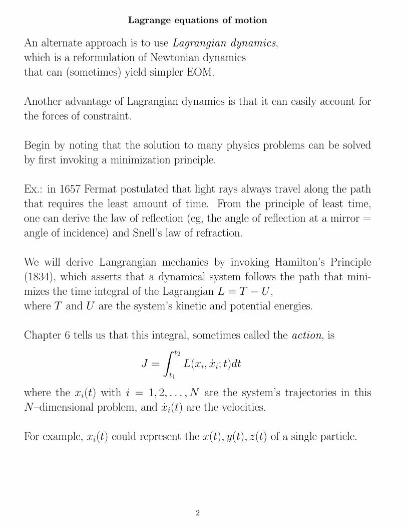
Lagrange equations of motion

An alternate approach is to use Lagrangian dynamics,

which is a reformulation of Newtonian dynamics

that can (sometimes) yield simpler EOM.

Another advantage of Lagrangian dynamics is that it can easily account for

the forces of constraint.

Begin by noting that the solution to many physics problems can be solved

by first invoking a minimization principle.

Ex.: in 1657 Fermat postulated that light rays always travel along the path

that requires the least amount of time. From the principle of least time,

one can derive the law of reflection (eg, the angle of reflection at a mirror =

angle of incidence) and Snell’s law of refraction.

We will derive Langrangian mechanics by invoking Hamilton’s Principle

(1834), which asserts that a dynamical system follows the path that mini-

mizes the time integral of the Lagrangian L = T − U ,

where T and U are the system’s kinetic and potential energies.

Chapter 6 tells us that this integral, sometimes called the action, is

J =

∫ t2

t1

L(xi, xi; t)dt

where the xi(t) with i = 1, 2, . . . , N are the system’s trajectories in this

N–dimensional problem, and xi(t) are the velocities.

For example, xi(t) could represent the x(t), y(t), z(t) of a single particle.

2

Hamilton’s Principle implies that the action J has a minimum along the

system’s trajectory xi(t).

Consequently, each of the trajectories xi(t) obey the Euler–Lagrange eqn’s:

∂L

∂xi−

d

dt

(

∂L

∂xi

)

= 0

These equations are usually called the Lagrange eqn’s.

Note that Newton’s Law can be recovered from the Lagrange eqn’s:

Consider the 1D motion of a particle moving in the potential U = U(x):

L(x, x) = T − U =1

2mx2 − U(x)

so∂L

∂x= −

∂U

∂x= F

thus F =d

dtmx = mx as expected.

Note that the Lagrange EOM are a reformulation of Newtonian mechanics.

They do not introduce any new physics. Rather, they merely provide an

alternate approach to solving physical problems.

Note also that Lagrangian dynamics does not deal with forces,

which are vector quantities;

rather, it deals with energies, which are scalars

(which can also be simpler to formulate).

3

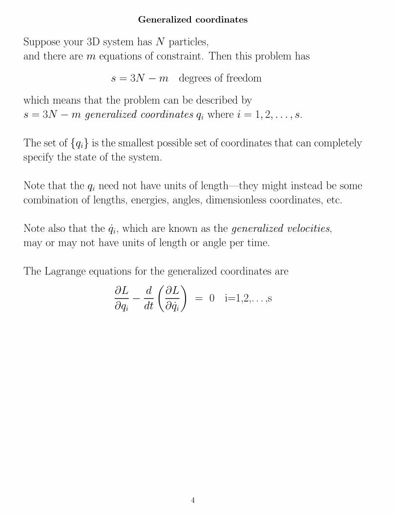
Generalized coordinates

Suppose your 3D system has N particles,

and there are m equations of constraint. Then this problem has

s = 3N − m degrees of freedom

which means that the problem can be described by

s = 3N − m generalized coordinates qi where i = 1, 2, . . . , s.

The set of {qi} is the smallest possible set of coordinates that can completely

specify the state of the system.

Note that the qi need not have units of length—they might instead be some

combination of lengths, energies, angles, dimensionless coordinates, etc.

Note also that the qi, which are known as the generalized velocities,

may or may not have units of length or angle per time.

The Lagrange equations for the generalized coordinates are

∂L

∂qi−

d

dt

(

∂L

∂qi

)

= 0 i=1,2,. . . ,s

4

Example 7.5

A pendulum is attached to a massless rim of radius a that rotates at a

constant angular velocity ω. Obtain the Lagrange equation for mass m.

Fig. 7–3.

5

Begin by writing the Lagrangian L = T − U .

What is this system’s potential energy U?

We will need m’s Cartesian coordinates:

x = a cos ωt + b sin θ

y = a sin ωt − b cos θ

What is T ?

Also need m’s velocities:

x = −aω sin ωt + b cos θθ

y = aω cos ωt + b sin θθ

so v2 = x2 + y2 = (aω)2 + (bθ)2 + 2abωθ(− cos θ sin ωt + sin θ cos ωt)

but right () = sin(θ − ωt)

so T =1

2mv2 =

1

2m[(aω)2 + (bθ)2 + 2abωθ sin(θ − ωt)]

and L =1

2m[(aω)2 + (bθ)2 + 2abωθ sin(θ − ωt)] − mg(a sin ωt − b cos θ)

What are the generalized coordinates for this system?

The generalized velocities?

We could have written L in terms of x, y and x, y.

Are the generalized coordinates?

6

What is the Lagrange equation for this system?

∂L

∂θ−

d

dt

(

∂L

∂θ

)

= 0

where∂L

∂θ= mabωθ cos(θ − ωt) − mgb sin θ

and∂L

∂θ= mb2θ + mabω sin(θ − ωt)

sod

dt

(

∂L

∂θ

)

= mb2θ + mabω(θ − ω) cos(θ − ωt)

thus abωθ cos(θ − ωt) − gb sin θ − b2θ − abω(θ − ω) cos(θ − ωt) = 0

so θ +g

bsin θ =

a

bω2 cos(θ − ωt)

is the EOM.

This is the EOM for a pendulum that is driven

by an external torque (eg, the term on the right).

ie, the simple pendulum is recovered when ω = 0.

How would you solve the EOM?

Always keep in mind the distinction in the meaning of a partial derivative:

∂L

∂θ(1)

and a total derivative:d

dt

(

∂L

∂θ

)

(2)

If you confuse the two, your EOM will be wrong.

7

Example 7.7—constrained motion

A bead of mass m slides along a parabolic wire where z = cr2.

The wire rotates with angular velocity ω about the vertical axis.

Obtain the system’s Lagrange eqn’s.

Also, how fast should the wire rotate in order to suspend the bead at an

equilibrium at height z > 0.

Fig. 7–5

The Lagrangian is

L = T − U

where U = mgz

T =1

2mv2

v = rr + rθθ + zz = bead’s velocity in cylindrical coord’s

so L =1

2m(r2 + r2θ2 + z2) − mgz

Is L written in terms of the system’s generalized coordinates?

8

How do I simplify this further using the constraint imposed by the wire?

First note that θ = ω,

and that z = cr2, so that z = 2crr and

L =1

2m(r2 + r2ω2 + 4c2r2r2) − mgcr2

What are this system’s generalized coordinates?

The Lagrange eqn’ is

∂L

∂r−

d

dt

(

∂L

∂r

)

= 0

where∂L

∂r= mrω2 + 4mc2rr2 − 2mgcr

and∂L

∂r= mr + 4mc2r2r

sod

dt

(

∂L

∂r

)

= mr + 8mc2rr2 + 4mc2r2r

so (1 + 4c2r2)r + 4c2rr2 − rω2 + 2gcr = 0

is the L’ EOM.

What is the condition for ‘floating’ the bead

at some equilibrium height z = cr2 > 0?

ie, how fast must the wire rotate for centrifugal force to balance gravity?

Since r = 0 and r = 0,

w2 = 2gc

is the angular at which the wire must spin in order to float the bead.

9

Example 7.9

A disk of mass M is constrained to roll down an inclined plane without

slipping. Solve the Lagrange equations for motion.

Fig. 6–7

First get the kinetic energy.

Recall from PHY305 that T = Tcenter of mass + Trot = 12My2 + Trot,

where Trot = 12Iθ2 is the KE due to the disk’s rotation,

I = 12MR2 = disk’s moment of inertia:

T =1

2My2 +

1

4MR2θ2

What is U?

The Lagrangian is then

L = T − U =1

2My2 +

1

4MR2θ2 + Mgy sin α

10

What does the no–slip constraint tell us about the coordinates y and θ?

What about the velocities?

Tip: put a dot on the disk, and use it to relate y ↔arclength.

y = Rθ and y = Rθ

This allows us to write L in terms of a single generalized coordinate:

L =3

4MR2θ2 + MgRθ sin α

The Lagrange equation for this system is

∂L

∂θ−

d

dt

(

∂L

∂θ

)

= 0

so MgR sin α =3

2MR2θ

ie θ =2g

3Rsin α

so θ(t) =2gt

3Rsin α assuming disk starts at rest

and θ(t) =gt2

3Rsin α

is the solution for the disk’s motion.

11

Problem Set #5

due Thursday November 10

at start of class

text problems 7–17, 7–27, 7–28, 7–33.

Exam #2

on Chapter 7 & Problem Sets 4 & 5

Thursday Nov. 17

The Hamiltonian H

Now lets derive another set of equations of motion from the Hamiltonian H .

This is usually obtained from the system’s Lagrangian:

begin by defining the generalized momentum pj ≡∂L

∂qj

the Lagrange Eqn. is then∂L

∂qj=

d

dt

∂L

∂qj= pj

Example: 1D motion of a single particle:

L =1

2mq2 − U(q)

p =∂L

∂q= mq

Note that p = the customary mass × velocity only when q is a length.

For other systems, p might instead be an angular momentum, or something

else.

Now construct the Hamiltonian H via the following equation:

H(pi, qi, t) =∑

j

pj qj − L(qi, qi, t)

where the sum extends over all of the pi & qi.

12

a simple example:

suppose L = L(x, y, x, y)

then px =∂L

∂xpy =

∂L

∂yand H(px, py, x, y) = pxx + pyy − L(x, y, x, y)

But note that H is defined to be a function of the p’s and q’s,

while L is ordinarily a function of q’s and q’s!

How do we exchange the q’s and q’s for p’s and q’s?

To write H as a function of the p’s and q’s, use pj = ∂L/∂qj to obtain an

equation for qj in terms of the p’s and q’s, ie, qj = qj(qi, pi, t).

Then replace each qj appearing in L with the equivalent expression

qj(qi, pi, t) that depends on the p’s and q’s

⇒this yields the Hamiltonian H(pi, qi, t) in its desired form.

13

Another set of EOM—Hamilton’s equations

To obtain the H’ EOM, start by calculating the total derivative of H :

H(pi, qi, t) =∑

j

pj qj − L(qi, qi, t)

so by Chain Rule, dH =∑

j

(

∂H

∂pjdpj +

∂H

∂qjdqj

)

+∂H

∂tdt

while derivative of RHS =∑

j

(

qjdpj + pjdqj −∂L

∂qjdqj −

∂L

∂qjdqj

)

−∂L

∂tdt

Note that∂L

∂qj= pj and

∂L

∂qj= pj,

so RHS =∑

j

(

qjdpj −∂L

∂qjdqj

)

−∂L

∂tdt

Think of dH as the total change in H that results when you alter the

pj, qj, and t by small, arbitrary displacements dpj, dqj, dt.

Next bring RHS→LHS:

∑

j

[(

∂H

∂pj− qj

)

dpj +

(

∂H

∂qj+ pj

)

dqj

]

+

(

∂H

∂t+

∂L

∂t

)

dt = 0

Since the displacements dpj, dqj, dt are arbitrary,

what does that tell us about their coefficients?

Thus we get Hamilton’s equations:

qj =∂H

∂pj

pj = −∂H

∂qj

∂H

∂t= −

∂L

∂t

⇒The system’s H tells you how its p’s and q’q evolve over time.

14

Suppose our system has s degrees of freedom,

ie, L is a function of s generalized coordinates.

The L’ EOM would thus yield s second–order DE’s,

while Hamilton’s Eqn’s would yield 2s first–order differential eqn’s.

Hamilton’s eqn’s provide yet another distinct set of EOM that are equivalent

to the Lagrange EOM and Newton’s Laws of motion.

Hamilton’s equations are especially useful in studies of

nonlinear & chaotic systems.

They are also quite handy when you want to draw a system’s phase diagram,

plots of the pi plotted versus the qi,

and are simply curves of constant H(pi, qi, t).

You will also need to know how to construct H in quantum mechanics,

since H appears in the Schrodinger eqn’.

15

The 7 Steps of H

Using Hamilton’s Eqn’s requires 7 steps:

1. Write L(qi, qi, t).

2. get the generalizes momenta

pj =∂L

∂qj

3. Use the above to solve for qj = qj(qi, pi, t).

4. Insert the above into L to express it as L(qi, pi, t).

5. Construct the Hamiltonian

H(pi, qi, t) =∑

j

pj qj − L(qi, pi, t)

6. Get Hamilton’s Eqn’s:

qj =∂H

∂pj

pj = −∂H

∂qj

7. solve, if possible

16

Example 7.11

Use Hamilton’s eqn’s to solve for the motion of a particle of mass m

that is subject to a spring–force F = −kr

while constrained to move on a cylinder of radius R.

Fig. 7–9.

1. obtain L = T − U :

U =1

2kr2 =

1

2k(x2 + y2 + z2)

How is U affected by the constraint?

⇒ x2 + y2 = R2 so U = 12k(R2 + z2).

The particle’s KE in cylindrical coordinates is

T =1

2m(r2 + r2θ2 + z2)

How does the constraint alter T ?

⇒ r = R and r = 0 so T = 12m(R2θ2 + z2).

17

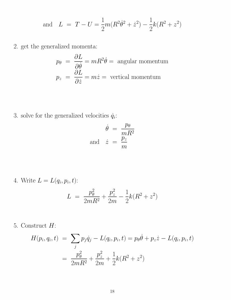
and L = T − U =1

2m(R2θ2 + z2) −

1

2k(R2 + z2)

2. get the generalized momenta:

pθ =∂L

∂θ= mR2θ = angular momentum

pz =∂L

∂z= mz = vertical momentum

3. solve for the generalized velocities qi:

θ =pθ

mR2

and z =pz

m

4. Write L = L(qi, pi, t):

L =p2

θ

2mR2+

p2z

2m−

1

2k(R2 + z2)

5. Construct H :

H(pi, qi, t) =∑

j

pj qj − L(qi, pi, t) = pθθ + pzz − L(qi, pi, t)

=p2

θ

2mR2+

p2z

2m+

1

2k(R2 + z2)

18

6. Get Hamilton’s Eqn’s:

qj =∂H

∂pjand pj = −

∂H

∂qj

so θ =∂H

∂pθ=

pθ

mR2and z =

∂H

∂pz=

pz

m

while pθ = −∂H

∂θ= 0 ⇒ angular momentum is conserved

and pz = −∂H

∂z= −kz

7. Solve for the motion.

Since pθ = constant, the particle revolves

with a constant angular velocity θ = pθ/mR2 ⇒ θ(t) = θt.

The equations for the vertical motions is that of a SHO:

z =pz

m= −

k

mz = −ω2

0z

so z(t) = A cos ω0t

19

H conservation

Recall that L = L(qi, qi, t). Thus by the Chain Rule,

dL

dt=

∑

j

(

∂L

∂qjqj +

∂L

∂qjqj

)

+∂L

∂t

but the Lagrange eqn’ is∂L

∂qj=

d

dt

∂L

∂qj

sodL

dt=

∑

j

(

qjd

dt

∂L

∂qj+

∂L

∂qjqj

)

+∂L

∂t

=∑

j

d

dt

(

qj∂L

∂qj

)

+∂L

∂t

but∂L

∂qj= pj

so∑

j

d

dt(qjpj − L) =

d

dt

∑

j

(qjpj − L) =dH

dt= −

∂L

∂t

thus if L is independent of t ⇒ H is conserved

when does H = E?

Next, show that H = E under certain circumstances:

now suppose∂L

∂t= 0

and U = U(qi) ie, U is independent of t and qi

what kind of system is this?

Also assume that T is a quadratic function of the q’s:

T (qi) =N

∑

j=1

N∑

k=1

aj,kqj qk where aj,k = ak,j

Examples include:

T =1

2m(x2 + y2 + y2) in Cartesian coord’s

or T =1

2m(r2 + r2θ2 + r2 sin2 θφ2) in spherical coord’s

20

Is T = 12m(x2 + xy + vz) quadratic in the generalized velocities?

Now show that H = E in this case:

since H =N

∑

i=1

piqi − L

=N

∑

i=1

∂L

∂qiqi − T + U

=

N∑

i=1

∂T

∂qiqi − T + U

Now calculate

∂T

∂qi=

N∑

j=1

N∑

k=1

aj,k∂

∂qiqj qk

=N

∑

j=1

N∑

k=1

aj,k(δi,j qk + qjδk,i)

=N

∑

k=1

ai,kqk +N

∑

j=1

aj,iqj = 2N

∑

k=1

ai,kqk since aj,i = ai,j

consequently,

N∑

i=1

∂T

∂qiqi = 2

N∑

i=1

N∑

k=1

ai,kqiqk = 2T

and thus H = 2T − T + U = E

21

To summarize:

When (i.) ∂L/∂t = 0 ⇒ H = constant

But when (i.) ∂L/∂t = 0

and (ii.) U = U(qi)

and (iii.) T =∑

j,k aj,kqj qk ⇒ H = E = constant

When conditions i., ii., and iii. hold, you can readily obtain the system’s

Hamiltonian H by simply writing down the system energy E.

Just make sure that E is written as a function of the p’s and q’s rather than

the q’s and q’s—you still have to eliminate the q’s in favor of the p’s.

Nonetheless, using H = E to construct the Hamiltonian can be a bit easier

than using the formal definition of H =∑

i piqi − L.

Cyclic coordinates

The pair (qk, pk) are called canonical conjugates

and the transformation from

L(qi, qi, t) → H(qi, pi, t) is a canonical transformation.

A coordinate qk that does not appear in L or H is said to be cyclic.

Cyclic coordinates are especially handy in Hamilton’s eqn’s since

pj = −∂H

∂qj= 0

⇒ the momenta of cyclic coordinates are constants of the motion.

22

Problem 7–28

A particle of mass m moves in the central force–field F (r) = −k/r2.

What are the Hamilton EOM?

What coordinate system should I use?

The PE for this system is U(r) = −k/r, which recovers F = −∂U/∂r.

What is the KE in this coordinate system?

The Lagrangian is

L = T − U =1

2m(r2 + r2θ2) +

k

r

So the system’s momenta are

pr =∂L

∂r= mr so r =

pr

m

and pθ =∂L

∂θ= mr2θ so θ =

pθ

mr2

Can we simply use H = E = T + U to construct the system’s Hamiltonian?

What 3 conditions must be met?

(i) is ∂L/∂t = 0?

(ii) is the system conservative, ie, is U = U(qi)?

(iii) is T quadratic in the qi’s?

23

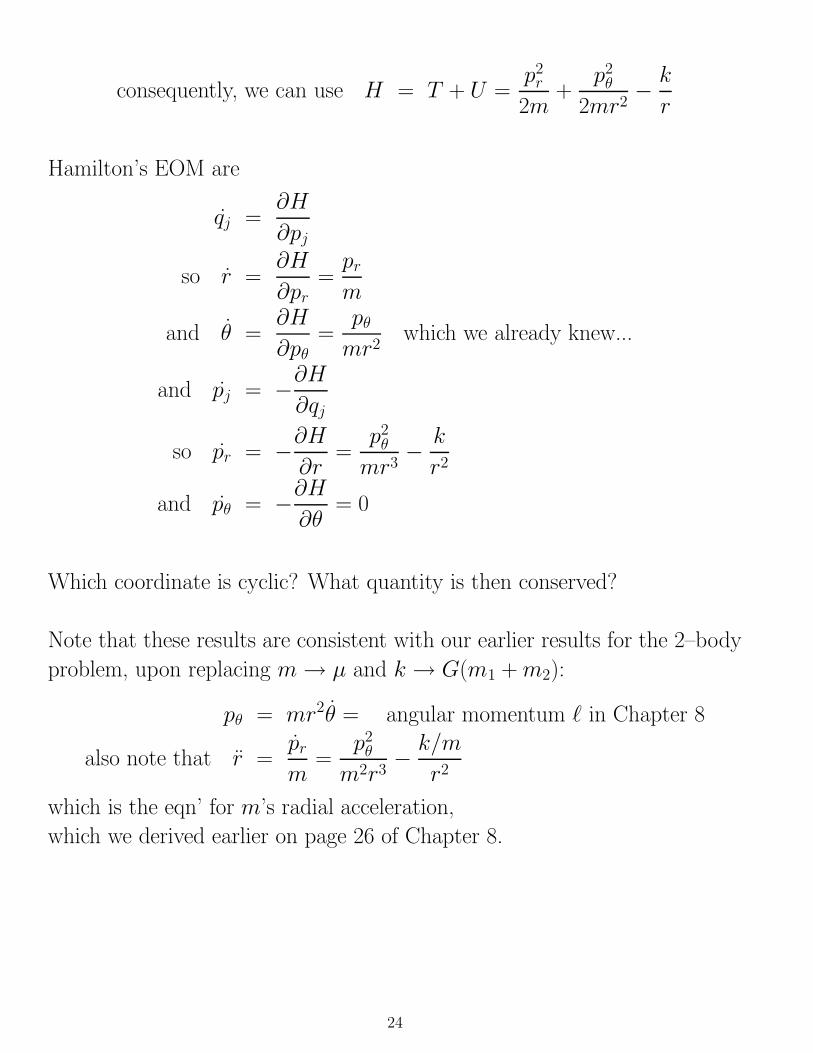
consequently, we can use H = T + U =p2

r

2m+

p2θ

2mr2−

k

r

Hamilton’s EOM are

qj =∂H

∂pj

so r =∂H

∂pr=

pr

m

and θ =∂H

∂pθ=

pθ

mr2which we already knew...

and pj = −∂H

∂qj

so pr = −∂H

∂r=

p2θ

mr3−

k

r2

and pθ = −∂H

∂θ= 0

Which coordinate is cyclic? What quantity is then conserved?

Note that these results are consistent with our earlier results for the 2–body

problem, upon replacing m → µ and k → G(m1 + m2):

pθ = mr2θ = angular momentum ` in Chapter 8

also note that r =pr

m=

p2θ

m2r3−

k/m

r2

which is the eqn’ for m’s radial acceleration,

which we derived earlier on page 26 of Chapter 8.

24