Lecture IV. Ecology I:

Population Growth and Demography

Apocalypse now. The Santa Ana Watershed Project Authority

pulls no punches in portraying its mission in apocalyptic terms.

The original horsemen were Conquest, War, Famine and Death.

2

Exponential Growth.

In an unlimited environment,

𝑑𝑁

𝑑𝑡= 𝑟𝑁 (1a)

𝑁(𝑡) = 𝑁0𝑒𝑟𝑡 (1b)

1. 𝑁(𝑡) is population size (or

density) at time t.

2. 𝑁0 is the initial size (densi-ty).

3. 𝑟 is the per capita rate of increase, i.e,, per individual

rate of births – deaths.

4. 𝑟 > 0: Population grows without bound.

5. 𝑟 < 0: Population collapses to 𝑁 = 0.

Needless to say – there are no unlimited environments. A typical bacterium dividing every 15 minutes or so would become a ball of cells the size of the earth in a couple of weeks!

Top. Population growth in an unlimited environment (theo-ry). Bottom. Bacterial cells in culture (real world).

3

Regarding bacterial growth:

1. Lag phase is due to bio-chemical “gearing-up.” – e.g., synthesis of inducible enzymes when cells grown on minimal medium.

2. Log phase, i.e., the period

of ~ exponential growth – so-called because

ln𝑁 = ln𝑁0 + 𝑟𝑡 (1c)

where 𝑁0 is the initial size of the population.

3. Stationary phase – cells alive but don’t reproduce due to resource depletion and accumulating waste products, toxins, etc.

4. Death phase – cells begin to die.

The fact that population growth comes to a halt indicates that Eqs. (1) appropriate only when numbers are small, i.e., during initial phase of population growth.

Bacterial cells in culture.

4

Age Structure. In most populations, individuals not all the same.

The young and the old typically manifest 1. Increased mortality;

2. Decreased fertility.

Survivorship curves ideal-ized as Types I (man); II (birds); III (fish) – Note the log scale.

Variation in mortality reflects 1. Vulnerability of the young. 2. Senescence (aging).

Variation in fertility reflects 1. Onset of sexual maturity.

2. Senescence.

Exceptions: Species with in-determinate growth, e.g. fish.

Age specific rates of year to tyear survival (top) and fertility (bottom).

5

Long-term per capita rate of population increase, r, de-termined by age-specific schedules of reproduction and survivorship. Approximately,

𝑟 ≈1

𝑇ln(𝑅0) (2)

1. 𝑅0 : Lifetime expectation of offspring.

2. 𝑇: Mean age of reproduction.

3. Formulas1:

𝑅0 =∑ℓ𝑥𝑚𝑥

(3)

𝑇 =∑𝑥ℓ𝑥𝑚𝑥

∑ℓ𝑥𝑚𝑥=∑𝑥ℓ𝑥𝑚𝑥

𝑅0

where 𝑥 is age, ℓ𝑥is the probability of surviving from birth to age 𝑥 and 𝑚𝑥 is the fertility of an x year-old.

1 Will be given on exam.

6

Stable Age Distribution (SAD). 1. If reproduction and mortality rates do not change with

time, population age structure will tend to a stable dis-

tribution as 𝑡 → ∞. Specifically,

𝑛𝑥

𝑛0=

ℓ𝑥

𝑒𝑟𝑥 (4)

where 𝑛0 and 𝑛𝑥 are the numbers of young of the year and individuals of age x.

2. Eq (4) gives proportions, not absolute numbers. 3. Important to distinguish between age distribution at any

particular time and the SAD.

4. Following a perturbation, the population will eventually return to the SAD, provided original fertility / survivorship schedules restored under most conditions.

5. Perturbations affecting human age structure include

a. Wars, famine, disease. b. Post WWII baby boom.

Changing age distributions can have important societal consequences, e.g., social security trust fund insolvency.

7

Population Waves Following a Perturbation.

Following a change in fertility or mortality schedules, populations converge to a new SAD provided the new rates remain unchanged.

8

Human Populations. Demographic Transition.

1. Economic development accompanied by a. Reduced mortality.

b. Reduced fertility.

2. Shifts age structure toward

older age classes.

3. In terms of 𝑛𝑥

𝑛0=

ℓ𝑥

𝑒𝑟𝑥 , (4)

a. Reduced fertility:

𝑒𝑟𝑥 ↓⇒𝑛𝑥

𝑛0↑

b. Reduced mortality:

ℓ𝑥 ↑↑;𝑒𝑟𝑥 ↑⇒

𝒏𝒙

𝒏𝟎 ↑

where ↑↑signifies a larger increase than ↑.

Top. Demographic transition. Value of r covaries with the vertical extent of the shaded region. Bottom. Declining Japanese fertility rates.

9

Demographic Dividend (DD).

1. Increasing ratio of workers to dependent age classes in-creases per capita productivity – important contributing factor to the “Asian miracle”.

2. A limited window of opportunity. a. Eventually population shifts to new structure with in-

creasing proportion of older dependent age classes. b. A problem now faced by most developed countries

Second Demographic Transition – Fertility drops below replacement values – Western Europe, Russia, etc.

10

Human Population Projections

World population past and projected. Three United Nations’ (2010) projections reflecting differing assumptions regarding future fertility human. In none of these scenarios is population growth exponential, i.e., with constant fertility, which is actually declining, world population would rise to ~26 billion by 2100.

11

World population projections out to 2300 reflecting different assumptions

regarding fertility (TFR) and population size in 2050 (low / high). Note

the projected collapse of human population consequent to continuing de-

clines in fertility. Also noteworthy is the sensitivity of the projections to

small differences in assumptions. Such sensitivity to parameter values is

what one expects in the case of exponentially growing populations. i.e.,

they either collapse or “blow up”. The paper (Lutz, 2008) from which this

figure is taken criticizes UN forecasts for assuming a floor TFR of 1.85

children. An additional major source of uncertainty (not shown here) is

life expectancy, which has been increasing globally at a rate of roughly

two years per decade. The projections shown here assume continuing

growth at this rate until an LE of 90 years is achieved.

12

Finite Environment.

Replace Equation 1 with

𝑑𝑁

𝑑𝑡= 𝐹(𝑁) (5)

For large N,

𝑑𝐹(𝑁)

𝑑𝑁< 0 (6)

i.e., rate of population growth declines with increasing population size.

1. Reflects resource limitation, which => increased mortali-ty and reduced fecundity at high densities.

2. Simplest formulation is the so-called logistic equation.

𝑑𝑁

𝑑𝑡= 𝑟𝑁(1 −

𝑁

𝐾) (7)

a. r as before.

b. K, the “carrying capacity” of environment, is a sta-

ble equilibrium, sometimes written 𝑁 = 𝑁∗.

13

Population growth and density. Top. Logistic growth. There is a single stable equilibrium. Bottom. Especially in social species, a minimum number of individuals may be required for the popula-tion to grow – think pack hunters such as wolves. This is called an “Allee effect,” the result of which is two stable equilibria.

14

Population Growth in Laboratory Microcosms.

G. F. Gause studied single species growth (yeast, para-mecia, etc.) in laboratory “microcosms.

Termination of growth due to accumulation of waste prod-ucts in a closed environment.

Single species experiments with yeasts. Left. Population growth comes to a halt with increasing concentrations of ethanol (waste prod-uct of glycolysis). Right. Equilibrial density declines with the addition of ethanol at the beginning of the experiment. From Gause, G. F. 1934. The Struggle for Existence. Hafner, NY.

15

DD vs. DI Mortality. 1. Assume density depend-

ent (DD) and density inde-pendent (DI) mortality.

2. Like r, rate of DI mortality, call it D, is computed per individual. Then

𝑑𝑁

𝑑𝑡= 𝐹(𝑁) − 𝐷 × 𝑁 (8)

3. Population still equilibrates, but at lower density, 𝑁∗ < 𝐾.

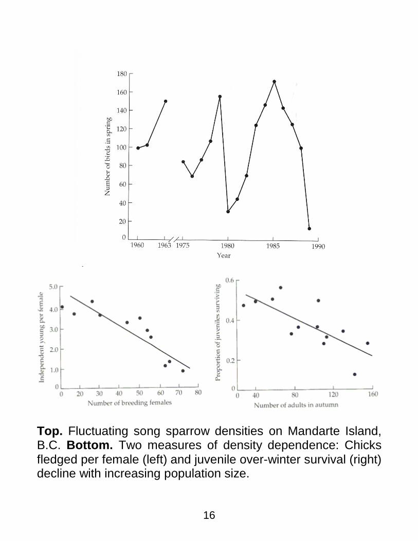
4. Widely Cited Example: song sparrow population fluctu-ations the result of varying rates of DI (cold winters).

5. Fluctuations unveil underlying density dependence. a. Larger spring populations reduce nestling survival. b. Larger fall populations reduce juvenile over-winter

survival.

4. Ecologists imagine that population size would stabilize absent fluctuating DI mortality.

5. There are, however, other possible causes of continuing fluctuations – e.g., interactions with other species.

16

Top. Fluctuating song sparrow densities on Mandarte Island, B.C. Bottom. Two measures of density dependence: Chicks fledged per female (left) and juvenile over-winter survival (right) decline with increasing population size.

17

Harvesting Renewable Resources.

Assume constant rate of re-source species removal, e.g., of fish, by commercial fish-ermen.

𝑑𝑁

𝑑𝑡= 𝐹(𝑁) − 𝐻 (9)

Two possibilities:

1. 𝐻 < 𝐻𝑚𝑎𝑥 = max[𝐹(𝑁)].

a. Two equilibria.

b. 0 < 𝑁‡(unstable) < 𝑁∗(stable).

2. 𝐻 > 𝐻𝑚𝑎𝑥. a. No equilibria.

b. Population → extinct.

𝐻𝑚𝑎𝑥 is called the maximum sustainable yield (MSY).

Harvesting at 𝐻 = 𝐻𝑚𝑠𝑥 maximizes both 1. Rate of resource acquisition. 2. Vulnerability to extinction.

Logistic growth with constant removal. Units of 𝑯are individ-uals/time. Compare with the units of 𝑫 in Equation (8).

18

If the environment fluctuates from one year to the next, harvesting at or near the maximum sustainable rate in most years will result in (local) resource extinction in a bad year.

19

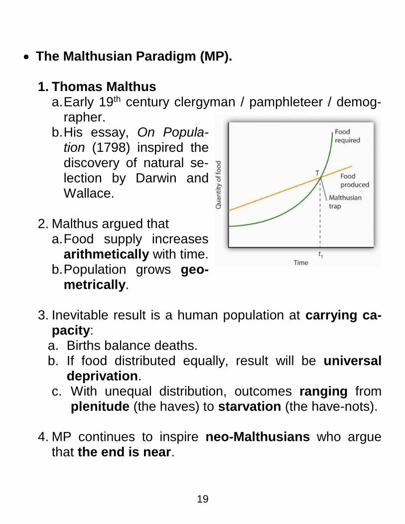
The Malthusian Paradigm (MP).

1. Thomas Malthus a. Early 19th century clergyman / pamphleteer / demog-

rapher. b. His essay, On Popula-

tion (1798) inspired the discovery of natural se-lection by Darwin and Wallace.

2. Malthus argued that

a. Food supply increases arithmetically with time.

b. Population grows geo-metrically.

3. Inevitable result is a human population at carrying ca-

pacity: a. Births balance deaths. b. If food distributed equally, result will be universal

deprivation. c. With unequal distribution, outcomes ranging from

plenitude (the haves) to starvation (the have-nots). 4. MP continues to inspire neo-Malthusians who argue

that the end is near.

20

From The Population Bomb (Ehrlich, 1968)

1. “The battle to feed all of humanity is over. In the 1970s and 1980s hundreds of millions of people will starve to death … At this late date [1968] nothing can prevent a substantial increase in the world death rate..." [p. xi. Emphasis added]

2. "a minimum of ten million people, most of them chil-

dren, will starve to death during each year of the 1970s. But this is a mere handful compared to the numbers that will be starving before the end of the century." [p. 3. Emphasis added]

3. “A cancer is an uncontrolled multiplication of cells; the

population explosion is an uncontrolled multiplication of people. Treating only the symptoms of cancer may make the victim more comfortable at first, but eventually he dies … . A similar fate awaits a world with a population explosion if only the symptoms are treated. We must shift our efforts from treatment of the symptoms to the cutting out of the cancer.” [p.152. Emphasis add-ed]

In a later publication, Ecoscience: Population, Resources, Environment, Ehrlich, Ehrlich & Holdren (1977) discussed the feasibility of adding sterilants to drinking water, the target being human, as opposed to bacterial reproduction.

21

All these Dire Predictions Failed – Why?

1. Ehrlich et al. imagined. a. Undiminished population growth. b. Constant or declining resource availability.

2. In fact,

a. The world’s population continued to grow, though more slowly than anticipated.

b. Food production / resource availability more than kept pace – Green Revolution.

c. In terms of Eq (7), human carrying capacity in-creased.

d. Consequence of energy / technological advances.

3. Regarding population: a. World fertility rate now below replacement level of

2.1 children / female – e.g., May (2007). b. If fertility continues to decline, world population will

almost certainly have peaked and be in decline by the end of the 21st century.

c. See pp. 10-11 RE forecasts and inherent sources of uncertainty.

4. Neo-Malthusians maintain it will have been too late,

a. Earth will be ravaged. b. Technological advance, unsustainable. c. Climate change, a “multiplier” – e.g., May (2007).

22

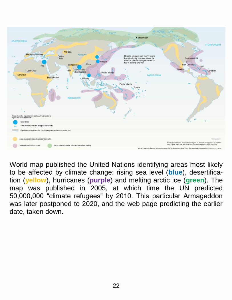
World map published the United Nations identifying areas most likely to be affected by climate change: rising sea level (blue), desertifica-tion (yellow), hurricanes (purple) and melting arctic ice (green). The map was published in 2005, at which time the UN predicted 50,000,000 “climate refugees” by 2010. This particular Armageddon was later postponed to 2020, and the web page predicting the earlier date, taken down.

23

Questions. 1. Assume that a population is growing exponentially, i.e.,

according to Equation 1a.

a. For r > 0, plot (𝑑𝑁 𝑑𝑡⁄ ) vs. N. Show that N = 0 is an un-stable equilibrium.

b. For r < 0, show that N = 0 is a stable equilibrium.

Note: Please review Lecture II.2 (p. 18) if you’ve forgotten the definition of stability.

2. Let r = 1.0, and the initial density, 𝑁0 = 1. Plot ln𝑁(𝑡) vs.

𝑡, for 𝑡 ranging from 0 to 100. What is the slope of the line?

3. Consider a partheno-genetic

population of females with the rates of survival and fertility shown at the right.

a. What is the mean age of

reproduction?

b. Estimate r.

c. What is the stable age distribution?

Age ℓx mx 0 1.00 0

1 0.90 0 2 0.80 0

3 0.70 1.0 4 0.40 2.0

5 0.10 2.0 6 0.00 -

24

4. How does changing one or more of the fertility values af-fect the SAD if r > 0?

5. Plot Equation 7 for values of N ranging from –K to +K. Do this for r > 0 and r < 0. Show that for r > 0, N=0 is an un-stable equilibrium, while for r < 0, N=0 is a stable equilibri-um. What happens when r = 0?

6. As shown at the right, the

proportion of male Mandarte song sparrows (“floaters”) unable to estab-lish territories increases with the number of territoreal males. This suggests that the number of territories is limited by physical factors such as avaliable space. Redraw the figure so as to contrast the following hypotheses. a. Territory size is incompressible, i.e., independent of the number of males hoilding territories. b. Territory size is in infintely elastic, .i.e.., varies inversely with the number of territorial males. Assume that the only thing that determines whether or not a male gets a territory is availability.

“Floaters” are males unable to establish to establish territo-ries.

25

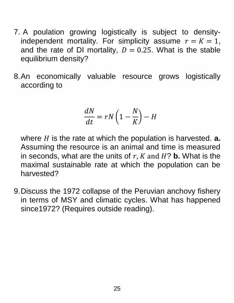
7. A poulation growing logistically is subject to density-

independent mortality. For simplicity assume 𝑟 = 𝐾 = 1, and the rate of DI mortality, 𝐷 = 0.25. What is the stable equilibrium density?

8. An economically valuable resource grows logistically

according to

𝑑𝑁

𝑑𝑡= 𝑟𝑁 (1 −

𝑁

𝐾) − 𝐻

where 𝐻 is the rate at which the population is harvested. a. Assuming the resource is an animal and time is measured

in seconds, what are the units of 𝑟,𝐾and𝐻? b. What is the maximal sustainable rate at which the population can be harvested?

9. Discuss the 1972 collapse of the Peruvian anchovy fishery in terms of MSY and climatic cycles. What has happened since1972? (Requires outside reading).