Martingale Ideas in Elementary Probability

Lecture courseHigher Mathematics College, Independent University of Moscow

Spring 1996

William FarisUniversity of Arizona

Fulbright Lecturer, IUM, 1995–1996

1

Preface

These lecture notes were distributed to students in the second year probability course at the HigherMathematics College, Independent University of Moscow, during the spring semester, 1996. They are anintroduction to standard topics in theoretical probability, including the laws of large numbers and thecentral limit theorem. The plan was to create a course that would cover this material without being a boringduplication of existing standard courses. Hence came the idea of organizing the course around the conceptof martingale. The elementary examples of martingales in the first part of the lectures are obtained byapplying gambling schemes to sums of independent random variables. The entire exposition makes no use ofthe concept of conditional probability and exposition, although these would be central to a more advanceddevelopment.

Alexander Shen and Alexei Melnikov were both helpful in the development of the course. In particular,Shen read an early version of the notes and contributed many insights. The students came up with severaloriginal solutions of the problems; among the most surprising were those by Kostya Petrov. Several of thestudents in the course helped with the final version of the notes. These included Alexander Cherepanov,Sam Grushevsky, Kostya Rutin, Dmitry Schwarz, Victor Shuvalov, and Eugenia Soboleva. Victor Shuvalovdeserves special mention; he was the organizer and a most able and enthusiastic participant.

The author was a Fulbright Lecturer at the Independent University of Moscow during the 1995–1996academic year. He thanks the faculty members of the university for their skillful arrangements and gen-erous hospitality. Alexei Roudakov, Yulii Ilyashenko, and Sergei Lando were extraordinarily helpful, andAlexei Sossinsky was particularly ingenious in solving all sorts of problems. Askol’d Khovanski and NikolaiKonstantinov were kind enough to include the author as a participant in their calculus seminar. It was aconstant pleasure to deal with such intelligent and well-organized people.

2

Contents

1. Introduction: Winning a fair game

2. The reflection principle

3. Martingales

4. The probability framework

5. Random variables

6. Variance

7. Independence

8. Supermartingales

9. The supermartingale convergence theorem

10. Dominated convergence theorems

11. The strong law of large numbers

12. Convergence of distributions

13. The central limit theorem

14. Statistical estimation

15. Appendix: Final examination

3

Lecture 1. Winning a fair game

Summary: Symmetric random walk is perhaps the most basic example of a fair game. For this gamethe strategy “play until you win a fixed amount” always succeeds in the long run. (Unfortunately one needsinfinite reserves and unlimited time to make this work in practice.)

I have no interest in games or gambling. However I am interested in probability models, especially inphysics, and hence in the notion of random fluctuation. One of the most important methods of studyingrandom fluctuations is to think of them as successive values of a fair game. Such a game is called a martingale,for reasons having to do with certain gambling schemes known by that name.

One of the most important ideas of this theory is that one cannot make gains without risk. We shallsee this illustrated over and over in the following lectures.

One unusual feature of these lectures is that I will develop martingale theory without the concept ofconditional expectation. Since the emphasis will be on simple concrete examples, there will not be muchemphasis on developing the theory of measure and integration. However the basic limit theorems will bepresented and illustrated.

Perhaps the most important probability model is that of Bernoulli trials. In this model there is anexperiment with various possible outcomes. Each such outcome is a sequence of values which are either asuccess S or a failure F . In other words, an outcome is a function from the indexing set of trials 1, 2, 3, . . .to the two element set S, F.

We first consider the most symmetric version of the model. An event is a set of outcomes to which aprobability is assigned. Consider a given function from the first n trials 1, 2, . . . n to S, F. Consider theevent A consisting of all outcomes that agree with this given function on the first n trials. This event isgiven probability 1/2n.

In general, if an event is a finite or countably infinite union of disjoint events, then the probability ofthis event is the corresponding sum of the probabilities of the constituent events.

Let Nn be the function from the set of outcomes to the natural numbers 0, 1, 2, 3, . . . that counts thenumber of successes in the first n elements of the outcome. Consider k with 0 ≤ k ≤ n. Let Nn = k denotethe event consisting of all outcomes for which the value of the function Nn is k. We have the fundamentalformula for the probability of k successes in n trials:

P[Nn = k] =(n

k

)12n. (1.1)

The derivation of this formula is simple. There is a bijective correspondence between the functions from1, . . . , n to S, F with exactly k successes and the subsets of the set 1, . . . , n with exactly k elements.The function corresponds to the subset on which the S values are obtained. However the number of k elementsubsets of an n element set is the binomial coefficient

(nk

). So the event Nn = k is the disjoint union of

(nk

)events each of which have probability 1/2n.

If one plots P[Nn = k] as a function of k for a fixed reasonably large value of n one can already startto get the impression of a bell-shaped curve. However we want to begin with another line of thought.

Let Sn = 2Nn − n. This is called symmetric random walk. The formula is obtained by counting 1 foreach success and −1 for each failure in the first n trials. Thus Sn = Nn − (n − Nn) which is the desiredformula. It is easy to see that

P[Sn = j] = P[Nn =n+ j

2] (1.2)

when n and j have the same parity.

We can think of Sn as the fortune at time n in a fair game. Of course Sn is a function from the set ofoutcomes to the integers.

4

Exercise 1.1. Show that P[S2m = 2r] → 0 as m → ∞. Hint: Write P[S2m = 2r] as a multiple ofP[S2m = 0]. For each r this multiple approaches the limit one as m → ∞. On the other hand, for each kthe sum for |r| ≤ k of P[S2m = 2r] is P[|S2m| ≤ 2k] ≤ 1.

Exercise 1.2. Fix k > 0. Find the limit as n→∞ of P[Sn ≥ k].

Exercise 1.3. Write k | m to mean that k divides m. It is obvious that P[2 | Sn] does not converge asn→∞. Does P[3 | Sn] converge as n→∞?

We want to see when we win such a game. Say that we want to win an amount r ≥ 1. Let Tr be thefunction from the set of outcomes to the numbers 1, 2, 3, . . . ,∞ defined so that Tr is the least n such thatSn = r. Thus Tr is the time when we have won r units.

Figure 1.

Example 1.1. Take r = 1. Then clearly P[T1 = 1] = 1/2, P[T1 = 3] = 1/8, P[T1 = 5] = 2(1/32), andP[T1 = 7] = 5(1/128). What is the general formula? What is the sum of these numbers?

Let us first look at the sum. This is the chance of ever getting from a fortune of zero to a fortune ofr > 0:

ρr = P[Tr <∞] =∞∑n=0

P[Tr = n]. (1.3)

We claim that ρr = 1; if you wait long enough you will win the game.

Here is a proof. The proof will use sophisticated reasoning, but the intuition is nevertheless compelling.We will later give other proofs, so one should not have too many worries yet about this point. The proof iscorrect, given enough theoretical background.

Clearly ρr = ρr1, since to win r units one has to have r independent wins of one unit. However usingthe same reasoning

ρ1 =12

+12ρ2 =

12

+12ρ2

1. (1.4)

This is because either at the first stage one immediately wins, or one immediately loses and then has to gainback two units. This is a quadratic equation that may be solved for ρ1. The only solution is ρ1 = 1.

This is a dramatic conclusion. In order to win in a fair game, one has only to wait until luck comesyour way. It almost surely will.

Exercise 1.4. Show if you start a symmetric random walk at an arbitrary integer point, then with proba-bility one it will eventually return to that point. This is the property of recurrence.

Exercise 1.5. Let mr ≥ 0 be the expected amount of time to get from an initial fortune of 0 to r. Clearlymr = rm1. Derive the formula

m1 =12

1 +12

(1 +m2). (1.5)

Solve the resulting linear equation.

Exercise 1.6. There is a non-symmetric version of the probability model in which the probability of successon each trial is p and the probability of failure on each trial is q and p+ q = 1. The probability of the set ofall infinite sequences of successes and failures that coincide on the first n trials with a fixed finite sequence

5

of length n is pkqn−k, where k is the number of successes in the finite sequence. Show that for this modelρr = ρr1 and

ρ1 = p+ qρ21. (1.6)

Find both solutions of this quadratic equation. Guess which solution is the correct probability to gain oneunit.

Exercise 1.7. In the preceding problem it is obvious what the correct solution must be when p > 1/2.A student in the course pointed out the following remarkable way of finding the correct solution whenp < 1/2. Let ρ1 be the probability that one eventually gains one unit, and let ρ−1 be the probability thatone eventually loses one unit. Show by examining the paths that ρ1 = p/qρ−1. On the other hand, one canfigure out the value of ρ−1.

Exercise 1.8. A non-symmetric random walk with p 6= 1/2 is not recurrent. Find the probability ofeventual return to the starting point.

Exercise 1.9. In the non-symmetric version derive the formulas mr = rm1 and

m1 = p1 + q(1 + 2m1). (1.7)

Find both solutions of this linear equation! Guess which solution is the correct expected number of steps togain one unit.

Exercise 1.10. Show that when p > q the expected time m1 =∑n nP[T1 = n] <∞. Hint: Compare with

the series ρ1 =∑n P[T1 = n] = 1 in the case p = 1/2.

Lecture 2. The reflection principle

Summary: The reflection principle is a special technique that applies to symmetric random walk. Itmakes it possible to calculate the probability of winning a specified amount in a fixed amount of time.

Recall that Sn for n = 1, 2, 3, . . . is a symmetric random walk. If r ≥ 1, then Tr is the first time n thatSn = r.

There is a remarkable explicit formula for probabilities associated with Tr. It is

P[Tr = n] =r

nP[Sn = r]. (2.1)

As time goes on, the probability that the walk visits r for the first time at n is a increasingly small proportionof the probability that the walk visits r at time n.

The formula is remarkable, but it does not cast much light on why the sum over n is one. Let us derivean equivalent version of the formula; that will give us a better idea of its meaning.

The way to get this formula is to derive instead a formula for P[Tr ≤ n]. The derivation is based onbreaking the event into two parts. We write

P[Tr ≤ n] = P[Tr ≤ n, Sn > r] + P[Tr ≤ n, Sn ≤ r] = P[Sn > r] + P[Tr ≤ n, Sn ≤ r]. (2.2)

Now we use the reflection principle:

P[Tr ≤ n, Sn ≤ r] = P[Tr ≤ n, Sn ≥ r]. (2.3)

Figure 2.

6

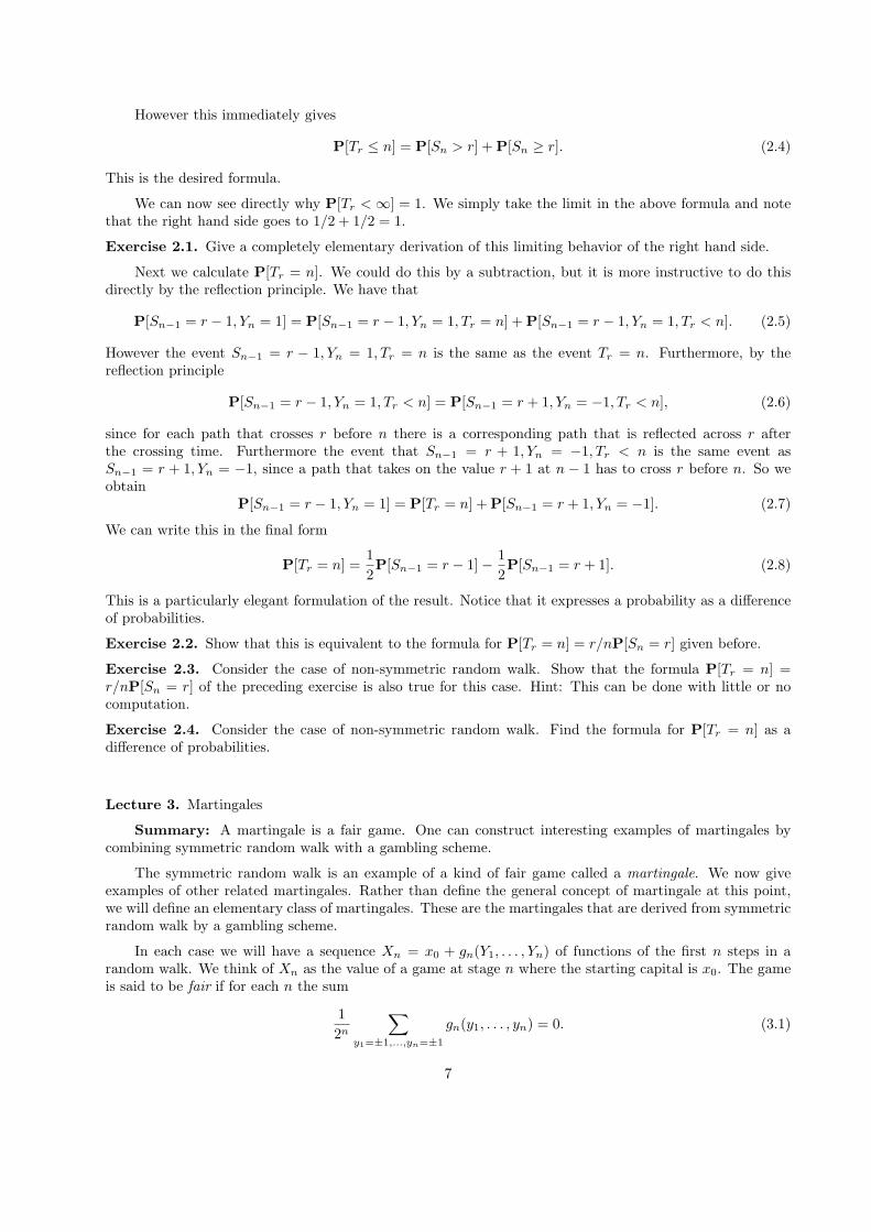
However this immediately gives

P[Tr ≤ n] = P[Sn > r] + P[Sn ≥ r]. (2.4)

This is the desired formula.

We can now see directly why P[Tr <∞] = 1. We simply take the limit in the above formula and notethat the right hand side goes to 1/2 + 1/2 = 1.

Exercise 2.1. Give a completely elementary derivation of this limiting behavior of the right hand side.

Next we calculate P[Tr = n]. We could do this by a subtraction, but it is more instructive to do thisdirectly by the reflection principle. We have that

P[Sn−1 = r − 1, Yn = 1] = P[Sn−1 = r − 1, Yn = 1, Tr = n] + P[Sn−1 = r − 1, Yn = 1, Tr < n]. (2.5)

However the event Sn−1 = r − 1, Yn = 1, Tr = n is the same as the event Tr = n. Furthermore, by thereflection principle

P[Sn−1 = r − 1, Yn = 1, Tr < n] = P[Sn−1 = r + 1, Yn = −1, Tr < n], (2.6)

since for each path that crosses r before n there is a corresponding path that is reflected across r afterthe crossing time. Furthermore the event that Sn−1 = r + 1, Yn = −1, Tr < n is the same event asSn−1 = r + 1, Yn = −1, since a path that takes on the value r + 1 at n − 1 has to cross r before n. So weobtain

P[Sn−1 = r − 1, Yn = 1] = P[Tr = n] + P[Sn−1 = r + 1, Yn = −1]. (2.7)

We can write this in the final form

P[Tr = n] =12P[Sn−1 = r − 1]− 1

2P[Sn−1 = r + 1]. (2.8)

This is a particularly elegant formulation of the result. Notice that it expresses a probability as a differenceof probabilities.

Exercise 2.2. Show that this is equivalent to the formula for P[Tr = n] = r/nP[Sn = r] given before.

Exercise 2.3. Consider the case of non-symmetric random walk. Show that the formula P[Tr = n] =r/nP[Sn = r] of the preceding exercise is also true for this case. Hint: This can be done with little or nocomputation.

Exercise 2.4. Consider the case of non-symmetric random walk. Find the formula for P[Tr = n] as adifference of probabilities.

Lecture 3. Martingales

Summary: A martingale is a fair game. One can construct interesting examples of martingales bycombining symmetric random walk with a gambling scheme.

The symmetric random walk is an example of a kind of fair game called a martingale. We now giveexamples of other related martingales. Rather than define the general concept of martingale at this point,we will define an elementary class of martingales. These are the martingales that are derived from symmetricrandom walk by a gambling scheme.

In each case we will have a sequence Xn = x0 + gn(Y1, . . . , Yn) of functions of the first n steps in arandom walk. We think of Xn as the value of a game at stage n where the starting capital is x0. The gameis said to be fair if for each n the sum

12n

∑y1=±1,...,yn=±1

gn(y1, . . . , yn) = 0. (3.1)

7

This just says that the expected value of the game at each stage is the starting capital.

Consider the steps Yi in the symmetric random walk, so Yi = ±1 depending on whether the ith trial isa success or a failure. Let x0 be the initial capital and set

Xn = x0 +W1Y1 +W2Y2 + · · ·WnYn, (3.2)

whereWi = fi(Y1, . . . , Yi−1). (3.3)

This is the elementary martingale starting at x0 and obtained by the gambling scheme defined by the fi. Theidea is that in placing the next bet at stage i one can make use of the information obtained by examiningthe results of play at stages before i. In many examples we take the starting capital x0 = 0.

Exercise 3.1. Show that an elementary martingale is a fair game.

Example 3.1. The symmetric random walk Sn is an elementary martingale.

Example 3.2. Let r ≥ 1 and let Tr be the time that the symmetric random walk hits r. Let Xn = Sn forn ≤ Tr and let Xn = r for n > Tr. This is the walk stopped at r. It is also an elementary martingale. Thisis a game that is played until a desired level of winnings is achieved.

Figure 3.

There is a general theorem that says that every martingale that is bounded above by some fixed constantmust converge with probability one. (It is also true that every martingale that is bounded below by somefixed constant must converge with probability one.) This example illustrates the theorem, since as we haveseen the probability is one that the martingale Xn converges to the constant value r as n→∞.

Notice that even though this game is fair at each n, it is not fair in the limit as n → ∞. In this limitthere is a sure gain of r. The explanation for this remarkable effect is that the martingale is not boundedbelow. The effect of a lower bound will be illustrated by the next example.

Example 3.3. Let q ≥ 1 and let T be the first time that the symmetric random walk hits either −q or r.Let Zn = Sn for n ≤ T and let Zn = ST for n > T . This is the random walk stopped at either −q or r. Itis also a martingale.

Figure 4.

There is another general theorem that says that a martingale that is bounded both below and abovenot only converges with probability one, but there is a sense in which the game stays fair in the limit. Thisexample illustrates this result, since (as we shall see) the limit of Zn as n → ∞ is −q with probabilityr/(r + q) and r with probability q/(r + q).

8

Examples 3.2 and 3.3 above are obtained by the same construction. Let T be the appropriate stoppingtime. Take Wi = 1 if i ≤ T and Wi = 0 if i > T . Notice that one can see whether i > T by looking at thevalues of Y1, . . . , Yi−1.

Exercise 3.2. Can one see whether i ≤ T by looking at the values of Y1, . . . , Yi−1?

Exercise 3.3. Can one see whether i ≥ T by looking at the values of Y1, . . . , Yi−1?

Exercise 3.4. Say that one were fortunate enough to have miraculous schemes in which Wi is allowed tobe a function of Y1, . . . , Yn. Show that the resulting Xn game could be quite unfair.

Now we give some more examples of martingales.

Example 3.4. Let Wi = 2Si−1 be the gambling scheme. Then

Xn = 2S1Y2 + 2S2Y3 + · · · 2Sn−1Yn = S2n − n. (3.4)

Exercise 3.5. Prove the last equality.

This example shows that S2n − n is also a fair game. This is perhaps one of the most fundamental and

useful principles of probability: random fluctuations of a sum of independent variables grow on the averageso that the square of the displacement is proportional to the number of trials.

Exercise 3.6. Prove that12n

∑y1=±1,...,yn=±1

(y1 + · · ·+ yn)2 = n. (3.5)

Example 3.5. Let Wi = 1/i. Then

Xn = Y1 +12Y2 +

13Y3 + · · ·+ 1

nYn. (3.6)

This example will turn out to be fundamental for understanding the “law of averages.” It is not abounded martingale, since if the Yi were all 1 the series would be a divergent series. However we shall seelater that the variance is bounded, and under this circumstances the martingale must converge. Thereforewe see that the sum

X = Y1 +12Y2 +

13Y3 + · · ·+ 1

nYn + · · · (3.7)

converges with probability one.

Exercise 3.7. In the preceding example, calculate Yn = Xn−(1/n)(X1 + · · ·+Xn−1) in terms of Y1, . . . , Yn.

Exercise 3.8. Does Yn arise as a martingale from the gambling scheme construction?

Exercise 3.9. Let xn → x as n→∞. Find the limit of zn = (1/n)(x1 + · · ·+ xn−1) as n→∞.

Example 3.6. Here is an example of the kind of gambling scheme that was called a “martingale”. LetYi = ±1 be the steps in a symmetric random walk. Let T be the first i such that Yi = 1. Let T ∧ n theminimum of T and n. Then

Zn = Y1 + 2Y2 + 4Y3 + . . . 2T∧n−1YT∧n. (3.8)

Thus one doubles the bet until a final win.

If T ≤ n then Zn = 1, since the last gain more than compensates for all the previous losses. This hasprobability 1 − 1/2n. However, if T > n, then Zn = 1 − 2n, which is a catastrophe. This has probability1/2n. The game is fair at each n. However the limit as n→∞ is 1, so in the limit it is no longer fair, justas in the case of random walk. (It converges faster than the random walk, but the risks of a long wait arealso greater.)

Example 3.7. Consider repeated trials of the gambling martingale of the last example with n = 1, 2, 3, . . .trials. This is a new martingale Z1, Z2, Z3, . . .. Observe that Zn = 1 with probability 1−1/2n and Zn = 1−2n

9

with probability 1/2n. Let Sn = Z1 + · · ·+Zn be the accumulated earnings. Let A be the event that Sn →∞as n→∞. Even though this is a fair game, the probability of A is P[A] = 1.

Figure 5.

In order to see this, let B be the event that Zn are eventually one for all large enough n. Clearly B ⊂ A.Furthermore, the complement Bc consists of all outcomes for which Zn 6= 1 for arbitrarily large n. Let Ckbe the event that there exists an n ≥ k such that Zn 6= 1. Then for each k we have Bc ⊂ Ck. Let Ckn bethe event that n is the first time n ≥ k such that Zn 6= 1. Since Ck is the union for n ≥ k of the disjointevents Ckn, we have

P[Ck] =∞∑

n=k

P[Ckn] ≤∞∑

n=k

P[Zn 6= 1] =1

2k−1. (3.9)

Hence P[Bc] ≤ P[Ck] ≤ 1/2k−1. Since k is arbitrary, we must have P[Bc] = 0. It follows that P[B] = 1,and so also P[A] = 1.

Notice that what makes this possible is the fact that there is no lower bound on the game. The gamblerhas to be willing initially to go into heavy debt.

Example 3.8. Let Nn be the number of successes in n independent trials when the probability of successon each trial is 1/2. Let Sn = 2Nn − n be the symmetric random walk. Let p be a number with 0 < p < 1and let q = 1− p. Then

Xn = (2p)Nn(2q)n−Nn = (√

4pq)n(√

p

q

)Sn(3.10)

is a martingale. (We multiply by 2p for each success, by 2q for each failure.)

Exercise 3.10. Show that Xn −Xn−1 = (p− q)YnXn−1.

Exercise 3.11. Show that Xn arises from the random walk martingale by a gambling scheme.

Exercise 3.12. A martingale that is bounded below converges with probability one. Clearly Xn ≥ 0. Thusthe event A that the limit of the martingale Xn as n → ∞ exists has probability one. That is, for eachoutcome ω in A there is a number X(ω) such that the limit as n → ∞ of the numbers Xn(ω) is X(ω).Suppose p 6= 1/2. Find the values of X on the outcomes in A.

Note: This sort of martingale is important in physics; it is one of the first basic examples in statisticalmechanics. In that context we might call Sn the energy and write

√p/q = e−β and call 1/β the temperature.

Then p− q = tanh(−β) and√

4pq = 1/ cosh(β), so this may be written

Xn =e−βSn

coshn β. (3.11)

It is called the canonical Gibbs density.

10

Lecture 4. The probability framework

Summary: The standard framework for probability experiments is a probability space. This consistsof a set of outcomes, a σ-field of events, and a probability measure. Given a probability space describing onetrial of an experiment, there is a standard construction of a probability space describing an infinite sequenceof independent trials.

We now describe the three elements of a probability space in some detail. First one is given a set Ω.Each point ω in Ω is a possible outcome for the experiment.

Second, one is given a σ-field of F subsets of Ω. Each subset A in F is called an event. Recall thata σ-field of subsets is a collection of subsets that includes ∅ and Ω and is closed under countable unions,countable intersections, and complements.

The event ∅ is the impossible event, and the event Ω is the sure event. (This terminology derives fromthe fact that an experiment is sure to have an outcome.)

Third and finally, one is given a probability measure P. This is a function that assigns to each event Aa probability P[A] with 0 ≤ P[A] ≤ 1. This is the probability of the event A. The probability measure mustsatisfy the properties that P[∅] = 0, P[Ω] = 1. It also must satisfy countable additivity: for every disjointsequence An of events P[

⋃nAn] =

∑n P[An]. It follows from this that the probability of the complement

Ac of an event A is given by P[Ac] = 1−P[A].

Exercise 4.1. Show that A ⊂ B implies P[A] ≤ P[B].

Exercise 4.2. Show that P[A ∪B] = P[A] + P[B]−P[A ∩B].

Exercise 4.3. Events A and B are said to be independent if P[A ∩B] = P[A]P[B]. Show that if A and Bare independent, then so are A and Bc.

Exercise 4.4. Show that if An are a sequence of events, the one has countable subadditivity

P[⋃n

An] ≤∑n

P[An]. (4.1)

We define the convergence of a sequence of events. We say that An → A if for every ω there exists anN such that for all n ≥ N , ω ∈ An if and only if ω ∈ A.

Exercise 4.5. Let An be an increasing sequence of events. Show that An → A as n → ∞ impliesP[An]→ P[A].

Exercise 4.6. Let An be a decreasing sequence of events. Show that An → A as n→∞ implies P[An]→P[A].

Exercise 4.7. Let An be a sequence of events. Show that An → A as n→∞ implies P[An]→ P[A].

We often indicate an event A (a subset of Ω) by a corresponding condition α (true or false depending onthe particular outcome ω ∈ Ω). The condition that α is true for the outcome ω is that ω ∈ A. Conversely,the subset A corresponding to the condition α is ω | α(ω). When conditions are combined by the logicaloperations α or β, α and β, not α, the corresponding sets are combined by the set theoretical operations ofunion, intersection, and complement: A ∪ B, A ∩ B, Ac. Similarly, for an existential condition ∃nαn or auniversal condition ∀nαn the corresponding set operations are the union

⋃nAn and intersection

⋂nAn.

In this context we often denote a conjunction or the intersection of sets by a comma, so that for instanceP[A,B] is the probability of the conjunction or intersection of the events A and B. Thus we might for instancewrite a special case of the additivity law as

P[A] = P[A,B] + P[A,Bc]. (4.2)

An event A is said to be an almost sure event if P[A] = 1. A large part of the charm of probabilityis that one can show that various interesting events are almost sure. Thus an event that is not a logical

11

necessity can nevertheless be a sure bet. Similarly, we could call an event A such that P[A] = 0 an almostimpossible event; this terminology is not as common, but it is quite natural.

Exercise 4.8. The event that An occurs infinitely often as n→∞ is⋂k

⋃n≥k An. The condition that the

outcome ω ∈ ⋂k⋃n≥k An is the same as the condition that ∀k∃nω ∈ An, so this event is the set of outcomes

for which the events in the sequence happen for arbitrarily large index. Prove the first Borel-Cantelli lemma:If∑n P[An] < ∞, then the event that An occurs infinitely often is almost impossible. Hint: For each k,

P[⋂k

⋃n≥k An] ≤ P[

⋃n≥k An].

Exercise 4.9. Do Exercise 3.7 using explicitly the first Borel-Cantelli lemma.

When an experiment is performed it has an outcome ω. If A is an event and ω is in A, then the eventis said to happen. The probability of an event A is a mathematical prediction about the proportion of timesthat an event would happen if the experiment were repeated independently many times. Whether or notthe event actually happens on any particular experiment is a matter of fact, not of mathematics.

Example 4.1. Discrete space; one trial. Let Ω1 be a countable set. Let F1 consist of all subsets of Ω1. Letp : Ω1 → [0, 1] be a function such that

∑x∈Ω1

p(x) = 1. This is called a discrete density. Define

P1[A] =∑

x∈Ap(x). (4.3)

This is a basic example of a probability space.

Example 4.2. Continuous space; one trial. Let Ω1 be the real line. Let F1 be the smallest σ-field containingall intervals. Let ρ ≥ 0 be an integrable function such that

∫∞−∞ ρ(x) dx = 1. This is called a density. Let

P1[A] =∫

A

ρ(x) dx. (4.4)

This is a second basic example.

Independent trial construction

Let Ω1 be a probability space for one trial of an experiment, say as in example 4.1 or example 4.2. LetΩ∞ be the set of all functions from the set of trials 1, 2, 3, . . . to Ω1. Each outcome ω in Ω∞ is a sequenceof outcomes ωi for i = 1, 2, 3, . . . in the space Ω1. The set Ω∞ is the set of outcomes for the repeated trialsexperiment. For each i, let Xi be the function from Ω∞ to Ω1 given by Xi(ω) = ωi.

If A is an event in F1 describing what happens on one trial, then for each i the event Xi ∈ A is an eventin the repeated trials experiment defined by what happens on the ith trial. Explicitly this event is the setof all sequences ω such that Xi(ω) = ωi is in A. Let F∞ be the smallest σ-field of subsets of Ω∞ containingall such events Xi ∈ A.

Let A1, A2, A3, . . . be a sequence of single trial events in F1. Then the events Xi ∈ Ai are each in F∞and specify what happens on the ith trial. The event

⋂i[Xi ∈ Ai] is an event in F∞ that specifies what

happens on each trial. The probability measure P∞ for independent repeated trials is specified by

P∞[⋂

i

[Xi ∈ Ai]] =∏

i

P1[Ai]. (4.5)

This says that the probability of the conjunction or intersection of events defined by distinct trials is theproduct of the probabilities of the events for the single trial experiments.

Note that if Ai = Ω1 is the sure event for one trial, then its probability is one, and so it does notcontribute to the product. Similarly, the event Xi ∈ Ω1 is the sure event for repeated trials, and so it doesnot change the intersection. This definition is typically used when all but finitely many of the events are thesure event; in this case all but finitely many of the factors in the product are one.

12

Example 4.3. Discrete space; independent trials. In this case the set of outcomes Ω∞ consists of allsequences of points each belong to the countable set Ω1. The probability of the set of all sequences whoseinitial n values are x1, . . . , xn is the product p(x1) · · · p(xn).

Example 4.4. Continuous space: independent trials. In this case the set of outcomes Ω∞ consists of allsequences of real numbers. The probability of the set Bn of all sequences ω whose initial n values lie in aset B in n dimensional space is P∞[Bn] =

∫Bρ(x1) · · · ρ(xn) dx1 · · · dxn.

Example 4.5. Bernoulli trials. This is the special case where the discrete space has two points. We beginwith the space S, F consisting of the possible outcomes from one trial, a success or a failure. The σ-fieldconsists of all four subsets ∅, S, F, and S, F. The discrete density assigns probability p to S andprobability q = 1− p to F .

Next we consider independent trials of this experiment. An outcome is a sequence of S or F results.Among the events are success on the ith trial and failure on the ith trial. We can also specify what happenson a sequence of trials. If we take any finite subset of the trials and specify success or failure on each of theelements of the subset, then the probability of this is pkqm−k, where k is the number of successes and m− kis the number of failures.

Let Nn be the number of successes on the first n trials. If we ask what is the probability of the eventNn = k of having k successes on the first n trials, then one should realize that this event is the union of

(nk

)events where the subset of the first n trials on which the k successes occur is specified. Thus the probabilityis obtained by adding pkqn−k that many times. We obtain the famous binomial distribution

P[Nn = k] =(n

k

)pkqn−k. (4.6)

Example 4.6. Normal trials. This is the classical example for continuous variables. Let

ρ(x) =1√

2πσ2exp(− (x− µ)2

2σ2). (4.7)

This is the Gaussian or normal density with mean µ and variance σ2. Consider independent trials wherethis density is used on each individual trial. An outcome of this experiment is a sequence of real numbers,and the probabilities of events are given by multiple integrals involving this Gaussian density.

This example is much used in statistics, in large part for convenience. However it also has a fundamentaltheoretical justification. We shall see later that martingales that are the sum of many contributions ofcomparable magnitude (and consequently do not converge) tend to have their behavior characterized by theGaussian law.

Exercise 4.10. Discrete waiting times. The probability space for one trial consists of the numbers1, 2, 3, . . .. Fix p with 0 < p ≤ 1 and let q = 1 − p. The probability of r is pqr−1. This rep-resents the waiting time for the next success. The probability space for repeated trials is all sequencesof such numbers. For each sequence ω let Wk(ω) be the kth number in the sequence. This representsthe additional waiting time for the next success after k − 1 previous successes. For each trial we haveP[Wk = r] = pqr−1. It follows by summation that P[Wk > r] = qr. Furthermore, by the independent trialconstruction P[W1 = r1, . . . ,Wn = rn] = P[W1 = r1] · · ·P[Wn = rn].

Let Tk = W1 + · · ·+Wk. This is the total waiting time for the kth success. Find P[Tk = r]. Hint: Sumover all possible values of W1, . . . ,Wn.

Exercise 4.11. Let Nn = maxm | Tm ≤ n be the number of successes up to time n. Find P[Nn = k].Hint: Nn = k is the same as Tk ≤ n,Wk+1 > n− Tk. Sum over all possible values of W1, . . . ,Wn.

Exercise 4.12. Continuous waiting times. The probability space for one trial consists of the real numberss ≥ 0. Fix λ > 0. The probability density is λ exp(−λs). The probability of waiting more than t is the integralds of this from t to infinity, which is exp(−λt). The probability space for repeated trials is all sequences of

13

positive real numbers. For each sequence ω, let Wk(ω) be the kth number in the sequence. This is the waitingtime for the next arrival after k−1 previous arrivals. For each trial we have P[s < Wk < s+ds] = exp(−λs) dsand consequently P[t < Wk] = exp(−λt). Furthermore, the probabilities for distinct trials multiply.

Let Tk = W1 + . . .+Wk be the total waiting time for the kth arrival. Show that

P[t < Tk] =k−1∑m=0

(λt)m

m!e−λt. (4.8)

Hint: Show thatP[t < Tk] = P[t < Tk−1] + P[t− Tk−1 < Wk, Tk−1 ≤ t]

= P[t < Tk−1] +∫ t

0

P[t− s < Wk, s < Tk−1 ≤ s+ ds].(4.9)

and use P[t− s < Wk, s < Tk−1 ≤ s+ ds] = P[t− s < Wk]P[s < Tk−1 ≤ s+ ds].

Exercise 4.13. Let N(t) = maxr | Tr ≤ t be the number of arrivals up to t. Find P[N(t) = k].

Lecture 5. Random variables

Summary: A random variable assigns a number to each outcome of the experiment. Every positiverandom variable has a well-defined expectation. Random variables that are not positive may have well-defined expectations if there is no ambiguity involving infinity minus infinity.

Terminology note: I use the term positive to mean greater than or equal to zero. I use strictly positive tomean greater than zero. Similarly, increasing means that increments are positive; strictly increasing meansthat increments are strictly positive.

Consider a probability space with set of outcomes Ω, σ-field of events F , and probability measure P. Afunction X from Ω to the real numbers assigns an experimental number X(ω) to each outcome ω. We wantto make probability predictions about the values of such functions X.

Consider an interval I of real numbers. We would like to specify the probability P[X ∈ I] of the eventthat X has values in X. In other words, we would like the set of all outcomes ω such that X(ω) is in I tobe an event in the σ-field F . If this occurs for every interval I, then X is said to be a random variable, andP[X ∈ I] is well-defined.

When an experiment is performed, it has an outcome ω, and the value of the random variable for thatoutcome is an experimental number X(ω). Unfortunately probability theory does not tell us what thisnumber will be.

Example 5.1. Consider the Bernoulli trials example. Let Nn be the function from Ω to the natural numbersthat counts the number of successes in the first n trial. Then Nn = k is a condition that specifies an event inF . To see that this is an event in F , one notices that it is a union of

(nk

)disjoint events in F , each of which

is obtained as an intersection of events associated with individual trials. Thus we can legitimately computeP[Nn = k] =

(nk

)pkqn−k. For instance, when p = 1/2, P[S7 = 6] = 7/27 and P[S7 ≥ 6] = 7/27+1/27 = 1/16.

On January 1, 1996 I conducted 7 Bernoulli trials and for the outcome ω of that particular experimentN7(ω) = 6. The event that N7 ≥ 6 happened for that ω, but nothing in probability theory could havepredicted that.

If X is a random variable defined on a space Ω with probability measure P, then X defines a probabilitymeasure P1 defined for subsets of the real line by the formula by

P1[I] = P[X ∈ I]. (5.1)

This new probability measure is called the distribution of X. Much of classical probability theory consists ofcalculating the distributions of various random variables. The distribution of a random variable is nothing

14

more than a summary of the probabilities defined by that random variable in isolation from other randomvariables.

In some cases one can use a density to describe the distribution. This is when the associated probabilitymeasure can be represented by integrals of the form P1[I] =

∫Iρ(x) dx.

Exercise 5.1. Let X1 and X2 represent the results of the first two trials of the continuous independenttrials experiment. Show that the distribution of X1 +X2 is given by

P1[I] =∫

I

ρ2(y) dy, (5.2)

where the density ρ2 is given by the convolution integral

ρ2(y) =∫ ∞−∞

ρ(x)ρ(y − x) dx. (5.3)

If X is a random variable and f belongs to a very general class of functions (Borel measurable), thenf(X) is also a random variable. If X has density ρ, then it may be that f(X) also has a density, but thisdensity must be computed with an awkward change of variable. It is thus often convenient to continue touse the density of X for computations, as in the formula P[f(X) ∈ J ] =

∫x|f(x)∈J ρ(x) dx.

Each positive random variable X ≥ 0 has an expectation E[X] satisfying 0 ≤ E[X] ≤ ∞. If X is discrete,that is, if X has only a countable set S of values, then

E[X] =∑

x∈Sx ·P[X = x]. (5.4)

In the general case, for each ε > 0 let Xn be the random variable that has the value k/2n on the set whereX is in the interval [k/2n, (k + 1)/2n), for k = 0, 1, 2, 3, . . .. Then for each n the random variable Xn hasonly a countable sequence of values. Furthermore for each outcome the Xn values are increasing to thecorresponding X value, so the expectations E[Xn] are also increasing. We define

E[X] = limn

E[Xn]. (5.5)

Exercise 5.2. Let Nn be the number of successes in n Bernoulli trials where the probability of success oneach trial is p. Find E[Nn] from the definition.

Exercise 5.3. Let W be a discrete waiting time random variable with P[W > k] = qk. Find the expectationof W directly from the definition.

Exercise 5.4. Let W ≥ 0 be a continuous waiting time random variable such that P[W > t] = exp(−λt)with λ > 0. Find E[W ] from the definition.

Exercise 5.5. Let X be a positive random variable with density ρ. Prove from the definition that E[X] =∫∞0xρ(x) dx.

Exercise 5.6. Let W ≥ 0 be the continuous waiting time random variable with P[W > t] = exp(−λt).Find E[W ] by computing the integral involving the density.

Exercise 5.7. Let f(X) be a positive random variable such that X has density ρ. Prove that E[X] =∫∞−∞ f(x)ρ(x) dx.

Exercise 5.8. Compute E[W 2] for the continuous waiting time random variable.

Note: There are positive random variables that are neither discrete nor have a density. However theyalways have an expectation (possibly infinite) given by the general definition.

15

It is easy to extend the definition of expectation to positive random variables that are allowed to assumevalues in [0,∞]. The expectation then has an additional term ∞ · P[X = ∞]. This is interpreted with theconvention that ∞ · 0 = 0 while ∞ · c =∞ for c > 0.

With this convention we have the identity E[aX] = aE[X] for all real numbers a ≥ 0 and randomvariables X ≥ 0. Another useful and fundamental property of the expectation is that it preserves order: If0 ≤ X ≤ Y , then 0 ≤ E[X] ≤ E[Y ].

It is shown in measure theory that for a sequence of positive random variables Xi ≥ 0 we always havecountable additivity

E[∑

i

Xi] =∑

i

E[Xi]. (5.6)

The sum on the left is defined pointwise: For each outcome ω, the value of the random variable∑iXi on ω

is the number∑iXi(ω).

The notions of event and probability may be thought of as special cases of the notions of random variableand expectation. For each event A there is a corresponding random variable 1A that has the value 1 on theoutcomes in A and the value 0 on the outcomes not in A. The expectation of this indicator random variableis the probability:

E[1A] = P[A]. (5.7)

Exercise 5.9. Prove the most basic form of Chebyshev’s inequality: If Y ≥ 0, then for each ε > 0 we haveεP[Y ≥ ε] ≤ E[Y ].

Exercise 5.10. Let X ≥ 0 and let φ be an increasing function on the positive reals, for instance φ(x) = x2.Prove Chebyshev’s inequality in the general form that says that for ε > 0 we have φ(ε)P[X ≥ ε] ≤ E[φ(X)].

Exercise 5.11. Let 0 ≤ X ≤ M for some constant M and let φ be an increasing function. Prove thatE[φ(X)] ≤ φ(ε) + φ(M)P[X > ε].

Exercise 5.12. Show that countable additivity for probabilities is a special case of countable additivity forpositive random variables.

If we have a sequence of random variables, then we say Xn → X as n → ∞ if for every ω we haveXn(ω)→ X(ω) as n→∞.

Exercise 5.13. Prove that if Xn is an increasing sequence of positive random variables, and Xn → X, thenE[Xn]→ E[X].

Exercise 5.14. Consider this assertion: If Xn is a decreasing sequence of positive random variables, andXn → X, then E[Xn]→ E[X]. Is it true in general? Are there special circumstances when it is true?

If we have a random variable X that is not positive, then we can write it as the difference of two positiverandom variables X+ and X−. We can define

E[X] = E[X+]−E[X−] (5.8)

provided that at least one of the expectations on the right is finite. Otherwise we have an ambiguous∞−∞and the expectation is not defined. This is a not just a technical point; often much depends on whether anexpectation is unambiguously defined.

The absolute value of a random variable is |X| = X+ + X−. The absolute value |X| is also a randomvariable, and since it is positive, its expectation is defined. The expectation of X is defined and finite if andonly if the expectation of |X| is finite. In that case

|E[X]| ≤ E[|X|]. (5.9)

The expectation defined on the space of random variables with finite expectation is linear and order-preserving.

16

Example 5.2. Let X1, . . . , Xn represent the results of the first n trials of the discrete independent trialsexperiment. Let Y = f(X1, . . . , Xn). Then

E[Y ] =∑

x1,...,xn

f(x1, . . . , xn)p(x1) · · · p(xn). (5.10)

Example 5.3. Let X1, . . . , Xn represent the results of the first n trials of the continuous independent trialsexperiment. Let Y = f(X1, . . . , Xn). Then

E[Y ] =∫

Rn

f(x1, . . . , xn)ρ(x1) · · · ρ(xn) dx1 · · · dxn. (5.11)

If X is a random variable and P1 is its distribution, then there is an expectation E1 associated withthe distribution. It may be shown that E[f(X)] = E1[f ].

Exercise 5.15. If X1 and X2 are the results of the first 2 trials of the continuous independent trialsexperiment, show that

E[f(X1 +X2)] =∫ ∞−∞

f(y)ρ2(y) dy, (5.12)

where ρ2 is the convolution defined above.

Lecture 6. Variance

Summary: A random variable may be centered by subtracting its expectation. The variance of arandom variable is the expectation of the square of its centered version. This is a simple but powerfulconcept; it gives rise to a form of the law of averages called the weak law of large numbers.

A random variable is said to have finite variance if E[X2] < ∞. In this case its length is defined to be‖X‖ =

√E[X2].

Theorem 6.1 Schwarz inequality. If X and Y have finite variance, then their product XY has finiteexpectation, and

|E[XY ]| ≤ ‖X‖‖Y ‖. (6.1)

Proof: Let a > 0 and b > 0. Then for each outcome we have the inequality

±XYab

≤ 12

(X2

a2+Y 2

b2

). (6.2)

Since taking expectations preserves inequalities, we have

±E[XY ]ab

≤ 12

(‖X‖2a2

+‖Y ‖2b2

). (6.3)

Thus the left hand side is finite. Take a = ‖X‖ and b = ‖Y ‖.In the situation described by the theory we also write 〈XY 〉 = E[XY ] and call it the inner product of

X and Y .

If a random variable has finite variance then it also has finite expectation E[X] = 〈X〉 obtained bytaking the inner product with 1.

The mean of a random variable with finite expectation is defined to be

µX = E[X]. (6.4)

17

The variance of a random variable with finite variance is defined to be

Var(X) = σ2X = E[(X − µX)2]. (6.5)

Thus σ2X is the mean square deviation from the mean. The standard deviation σX is the square root of the

variance.

The following identity is not intuitive but very useful.

σ2X = E[X2]−E[X]2. (6.6)

The reason it is not intuitive is that it writes the manifestly positive variance as the difference of two positivenumbers.

Exercise 6.1. Prove it.

If X is a random variable with finite mean, then the centered version of X is defined to be X − µX . Ithas mean zero. Obviously the variance of X is just the square of the length of the centered version of X.

If X is a random variable with finite non-zero variance, then its standardized version is defined to be(X − µX)/σX . It has mean zero and variance one.

We define the covariance of X and Y to be

Cov(X,Y ) = E[(X − µX)(Y − µY )]. (6.7)

This is just the inner product of the centered versions of X and Y .

The correlation is the standardized form of the covariance:

ρXY =Cov(X,Y )σXσY

. (6.8)

This has the geometrical interpretation of the cosine of the angle between the centered random variables.

Again there is a non intuitive formula:

Cov(X,Y ) = E[XY ]−E[X]E[Y ]. (6.9)

Exercise 6.2. Prove it.

Two random variables are said to be uncorrelated if their covariance (or correlation) is zero. This saysthat the centered random variables are orthogonal.

Theorem 6.2 Let Sn = Y1 + · · ·Yn be the sum of uncorrelated random variables with finite variancesσ2

1 , . . . , σ2n. Then the variance of the sum is the sum σ2

1 + · · ·+ σ2n of the variances.

Exercise 6.3. Prove this (theorem of Pythagoras)!

Example 6.1. Say the means are all zero and the variances are all the same number σ2. Then Snis a generalization of the random walk we considered before. The theorem says that E[S2

n] = nσ2, or√E[S2

n] = σ√n. The random fluctuations of the walk are so irregular that it travels a typical distance of

only σ√n in time n.

Let Y1, . . . , Yn be uncorrelated random variables as above, all with the same mean µ. Define

Yn =Y1 + · · ·+ Yn

n(6.10)

to be the sample mean. Since this is a random variable, its value depends on the outcome of the experiment.For each n its expectation is the mean:

E[Yn] = µ. (6.11)

18

Theorem 6.3 The variance of the sample mean is

σ2Yn

=σ2

1 + · · ·+ σ2n

n2. (6.12)

In many circumstances the right hand side goes to zero. This says that the sample mean has small deviationfrom the mean. This is a form of the “law of averages”, known technically as the weak law of large numbers.

Assume that the variances of the Yi are all the same σ2. Then the variance of the sample mean isnσ2/n2 = σ2/n. The standard deviation of the sample mean is σ/

√n. It is exceedingly important to note

that while 1/√n goes to zero as n tends to infinity, it does so relatively slowly. Thus one needs a quite large

sample size n to get a small standard deviation of the sample mean. This 1/√n factor is thus both the

blessing and the curse of statistics.

Example 6.2. Consider discrete waiting times W1, . . . ,Wn, . . . with P[Wi = k] = pqk−1 for k = 1, 2, 3, . . .and with P[W1 = k1, . . . ,Wn = kn] = P[W1 = k1] · · ·P[Wn = kn]. The mean of Wi is µ = 1/p.

Exercise 6.4. Compute the mean from

µ =∞∑

k=1

kP[Wi = k]. (6.13)

For the discrete waiting time the variance is σ2 = q/p2.

Exercise 6.5. Compute the variance from

σ2 =∞∑

k=1

(k − µ)2P[Wi = k]. (6.14)

Notice that if p is small, then the standard deviation of the waiting time Wi is almost as large as themean. So in this sense waiting times are quite variable. However let Wn be the sample mean with samplesize n. Then the mean is still µ, but the standard deviation is σ/

√n. Thus for instance if p = 1/2, then the

mean is 2 and the standard deviation of the sample mean is√

2/n. A sample size of n = 200 should givea result that deviates from 2 by only something like 1/10. It is a good idea to perform such an experimentand get a value of Wn(ω) for the particular experimental outcome ω. You will either convince yourself thatprobability works or astonish yourself that it does not work.

Example 6.3. Consider the Bernoulli process. Let Yi = 1 if the ith trial is a success, Yi = 0 if the ith trialis a failure. The mean of Yi is p and its variance is p− p2 = pq.

Exercise 6.6. Compute this variance.

If i 6= j, then the covariance of Yi and Yj is p2 − p2 = 0.

Exercise 6.7. Compute this covariance.

Let Nn = Y1 + · · ·+ Yn be the number of successes in the first n trials. Then the mean of Nn is np andthe variance of Nn is npq.

Exercise 6.8. Compute the mean of Nn directly from the formula

E[Nn] =∑

k

kP[Nn = k] =∑

k

k

(n

k

)pkqn−k. (6.15)

Let Fn = Nn/n be the fraction of successes in the first n trials. This is the sample frequency. Thenthe mean of Fn is p and the variance of Fn is pq/n. We see from this that if n is large, then the samplefrequency Fn is likely to be rather close to the probability p.

19

It is more realistic to express the result in terms of the standard deviation. The standard deviation ofthe sample frequency is

√pq/√n.

This is the fundamental fact that makes statistics work. In statistics the probability p is unknown. Itis estimated experimentally by looking at the value of the sample frequency Fn (for some large n) on theactual outcome ω. This often gives good results.

Exercise 6.9. Say that you are a statistician and do not know the value of p and q = 1− p. Show that thestandard deviation of the sample frequency satisfies the bound

√pq√n≤ 1

2√n. (6.16)

Results in statistics are often quoted in units of two standard deviations. We have seen that an upperbound for two standard deviations of the sample frequency is 1/

√n.

Exercise 6.10. How many people should one sample in a poll of public opinion? Justify your answer. (Howlarge does n have to be so that 1/

√n is 3 per cent?)

The Bernoulli example is unusual in that the variance p(1 − p) is a function of the mean p. For moregeneral distributions this is not the case. Consider again a sequence of random variables Yi all with the samemean µ and variance σ2. Statisticians estimate the variance using the sample variance

Vn =(Y1 − Yn)2 + (Y2 − Yn)2 + · · ·+ (Yn − Yn)2

n− 1. (6.17)

It has the property that it requires no knowledge of the mean µ and is unbiased:

E[Vn] = σ2 (6.18)

Exercise 6.11. Prove this property. What is the intuitive reason for the n− 1 in the denominator? Woulda statistician who used n encounter disaster?

Exercise 6.12. The weak law of large numbers is also true if the covariances are not zero but merelysmall. Let Y1, . . . , Yn, . . . be a sequence of random variables with mean µ such that for j ≤ i we haveCov(Yi, Yj) ≤ r(i − j). Require that the bound r(k) → 0 as k → ∞. Show that the variance of the samplemean Yn goes to zero as n→∞.

Exercise 6.13. In the case of bounded variances and zero covariances the variance of the sample mean goesto zero like 1/n. Consider the more general weak law with a bound on the covariances. What kind of boundwill guarantee that the variance of the sample mean continues to go to zero at this rate?

Exercise 6.14. In this more general weak law there is no requirement that the negative of the covariancesatisfy such a bound. Are there examples where it does not?

Lecture 7. Independence

Summary: Some probability calculations only require that random variables be uncorrelated. Othersrequire a stronger martingale property. The strongest property of this sort is independence.

Recall that the condition that two random variables X and Y be uncorrelated is the condition that

E[XY ] = E[X]E[Y ]. (7.1)

Let Yc = Y −E[Y ] be the centered random variable. The condition that the random variables are uncorrelatedmay also be written in the form

E[XYc] = 0. (7.2)

20

There are stronger conditions that are very useful. One is the condition that for all functions f forwhich the relevant expectations are finite we have

E[f(X)Y ] = E[f(X)]E[Y ]. (7.3)

It says that Y is uncorrelated with every function of X. The condition is linear in Y but non-linear in X.In terms of the centered random variable Yc = Y −E[Y ] it says that

E[f(X)Yc] = 0. (7.4)

If we think of a game with two stages, and we think of weighting the bet Yc at the second stage with theresult of a gambling strategy f(X) based on the first stage result X, then this is the condition that themodified game remains fair, that is, that Yc be a martingale difference. For the purposes of this discussionwe shall call this the martingale property.

Exercise 7.1. Let Z have values 1 and 0 with equal probabilities, and let W have values 1 and −1 withequal probabilities, and let Z and W be independent. Show that X = ZW and Y = (1−Z) are uncorrelatedbut do not have the martingale property.

There is an even stronger condition. Two random variables are independent if for all functions f and gfor which the relevant expectations are finite,

E[f(X)g(Y )] = E[f(X)]E[g(Y )]. (7.5)

It says simply that arbitrary non-linear functions of X and Y are uncorrelated.

Exercise 7.2. Show that if X and Y are independent, and if I and J are intervals, then P[X ∈ I, Y ∈ J ] =P[X ∈ I]P[Y ∈ J ].

Exercise 7.3. Events A and B are said to be independent if their indicator functions 1A and 1B areindependent. Find a single equation that characterizes independence of two events.

Exercise 7.4. Let Z have values 1 and 0 with equal probabilities, and let W have values 1 and −1 withequal probabilities, and let Z and W be independent. Show that X = ZW and Y = (1 − Z)W have themartingale property but are not independent.

We can generalize all these definitions to a sequence Y1, . . . , Yn of random variables. The condition thatYn be uncorrelated with Y1, . . . , Yn−1 is that

E[(a1Y1 + · · ·+ an−1Yn−1 + b)Yn] = E[a1Y1 + · · ·+ an−1Yn−1 + b]E[Yn] (7.6)

for all choices of coefficients.

The condition that Yn −E[Yn] is a martingale difference is that

E[f(Y1, . . . , Yn−1)Yn] = E[f(Y1, . . . , Yn−1)]E[Yn] (7.7)

for all functions f . This says that even if the bet Yn−E[Yn] is weighted by a gambling scheme based on theprevious trials the expected gain remains zero.

The condition that Yn be independent of Y1, . . . , Yn−1 is that

E[f(Y1, . . . , Yn−1)g(Yn)] = E[f(Y1, . . . , Yn−1)]E[g(Yn)] (7.8)

for all functions f and g.

Exercise 7.5. Show that if we have a sequence Y1, . . . , Yn of random variables such that each Yj is inde-pendent of the Yi for i < j, then

E[f1(Y1) · · · fn(Yn)] = E[f1(Y1)] · · ·E[fn(Yn)] (7.9)

21

for all functions f1, . . . , fn.

Exercise 7.6. Say that we have three random variables Y1, Y2, and Y3 such that Y2 is independent of Y1

and such that Y3 is independent of Y1 and Y3 is independent of Y2. Must Y3 be independent of Y1, Y2?

How do we get random variables satisfying such conditions? The independence condition is the strongestof these conditions, so let us see if we can find independent random variables. Consider a probability spaceconstructed from an sequence of independent trials. If Yi depends on the ith trial, then Yn is independentfrom Y1, . . . , Yn−1.

It is easiest to see this in the discrete case. Then

E[f(Y1, . . . , Yn−1)g(Yn)] =∑

y1,...,yn

f(y1, . . . , yn−1)g(yn)P[Y1 = y1, . . . Yn = yn]. (7.10)

However this is the same as

E[f(Y1, . . . , Yn−1)]E[g(Yn)]

=∑

y1,...,yn−1

∑yn

f(y1, . . . , yn−1)g(yn)P[Y1 = Y1, . . . , Yn−1 = yn−1]P[Yn = yn]. (7.11)

The fact that the probability of the intersection event is the product of the probabilities is the definingproperty of the independent trials probability space.

In the continuous case one needs to use a limiting argument. We will leave this for another occasion.

It is certainly possible to have independent random variables that do not arise directly from the inde-pendent trials construction.

Example 7.1. Geometric waiting times. It is possible to construct a probability model in which discretewaiting times are directly constructed so that they will be independent. However it is also possible toconstruct instead the model for Bernoulli trials and see that the discrete waiting times arise as independentrandom variables, but not directly from the construction.

Let Y1, Y2, . . . , Yn, . . . be 1 or 0 depending whether the corresponding Bernoulli trial is a success or afailure. These random variables are independent, by their construction.

Let T0 = 0 and let Tr for r ≥ 1 be the trial on which the rth success takes place. Let Wr = Tr − Tr−1

be the waiting time until the rth success.

Exercise 7.7. Show that P[W1 = k] = qk−1p. This is the probability distribution of a geometric waitingtime. (Actually this is a geometric distribution shifted to the right by one, since the values start with 1rather than with 0.)

Exercise 7.8. Show that W1, . . . ,Wn are independent. Hint: Show that the probability of the intersectionevent P[W1 = k1, . . . ,Wr = kn] = P[W1 = k1] · · · [Wr = kn].

Exercise 7.9. Find P[Tr = n]. Hint: Tr = n if and only if Nn−1 = r − 1 and Yn = 1.

Exercise 7.10. Find the mean and variance of Tr.

Exercise 7.11. Consider uncorrelated random variables Y1, . . . , Yn each with mean µ and variances σ2. Wehave seen that the weak law of large numbers says that

E[(Yn − µ)2] =σ2

n. (7.12)

Show that

P[|Yn − µ| ≥ ε] ≤ σ2

nε2. (7.13)

22

Exercise 7.12. Consider independent random variables Y1, . . . , Yn, . . . each with the same distribution, inparticular each with mean µ and variance σ2. Assume that the fourth moment E[(Y1 − µ)4] is finite. Showthat

E[(Yn − µ)4] =1n4

nE[(Y1 − µ)4] +

(42

)(n

2

)σ4

. (7.14)

Be explicit about where you use independence.

Exercise 7.13. Show that in the preceding exercise we have

E[(Yn − µ)4] ≤ C

n2. (7.15)

Exercise 7.14. Continuing, show that

E[∞∑

n=k

(Yn − µ)4] ≤ C

k − 1. (7.16)

Exercise 7.15. Show thatP[∃nn ≥ k, |Yn − µ| ≥ ε] ≤ C

(k − 1)ε4. (7.17)

This remarkable result says that the probability that the sample mean ever deviates from the mean at anypoint in the entire future history is small. This is a form of the strong law of large numbers.

Exercise 7.16. Consider Bernoulli trials. Show that

P[∃nn ≥ k, |Fn − p| ≥ ε] ≤ 14(k − 1)ε4

(7.18)

for k ≥ 4. This says that no matter what the value of p is, for n large enough the sample frequencies Fn arelikely to get close to the probability p and stay there forever.

Lecture 8. Supermartingales

Summary: A martingale is a fair game. A supermartingale is a game that can be either fair orunfavorable. One can try to get a positive return with a supermartingale by a strategy of “quit when youare ahead” or of “buy low and sell high.” This strategy can work, but only in a situation where there is alsoa possibility of a large loss at the end of play.

A martingale is a fair game. It is useful to have a more general concept; a supermartingale is a gamethat is unfavorable, in that on the average you are always either staying even or losing.

Let S0 and Y1, Y2, Y3, . . . be a sequence of random variables with finite expectations. Let Sn = S0 +Y1 + · · ·+ Yn. We think of the Yi as the outcomes of the stages of a game, and Sn is the cumulated gain.

We want to specify when Sn is a supermartingale, that is, when the Yi for i ≥ 1 are supermartingaledifferences.

Let W1,W2,W3, . . . be an arbitrary gambling scheme, that is, a sequence of bounded random variablessuch that Wi ≥ 0 is a positive function of S0 and of Y1, . . . , Yi−1:

Wi = fi(S0, Y1, . . . , Yi−1). (8.1)

The requirement that the Yi for i ≥ 1 are supermartingale differences is that

E[WiYi] ≤ 0 (8.2)

23

for all i ≥ 1 and for all such gambling schemes. We take this as a definition of supermartingale; it turns outto be equivalent to other more commonly encountered definitions.

Notice that we can take as a special case all Wi = 1. We conclude that for a supermartingale differencewe always have

E[Yi] ≤ 0 (8.3)

for i ≥ 1. By additivity we haveE[Sn] ≤ E[S0]. (8.4)

On the average, the game is a losing game.

Example 8.1. Let S0, Y0, Y1, . . . , Yn, . . . be a sequence of independent random variables with finite expec-tations and with E[Yi] ≤ 0 for i ≥ 1. Then the partial sums Sn = S0 +Y1 + . . .+Yn form a supermartingale.In fact, if we have Wi = fi(S0, Y1, . . . , Yi−1) ≥ 0, then E[WiYi] = E[Wi]E[Yi] ≤ 0.

Theorem 8.1 Consider a supermartingale Sn = S0 + Y1 + · · · + Yn. Let X0 = f(S0) be a function of S0.Consider a gambling scheme Wi = fi(S0, Y1, . . . , Yi−1) ≥ 0. Form the sequence

Xn = X0 +W1Y1 +W2Y2 + · · ·WnYn. (8.5)

Then Xn is also a supermartingale.

The proof of the theorem is immediate. One consequence is that

E[Xn] ≤ E[X0]. (8.6)

All that a gambling scheme can do to a supermartingale is to convert it into another supermartingale, thatis, into another losing game.

There is a related concept of submartingale, which is intended to model a winning game, in which all ≤relations are replaced by ≥ relations. However this reduces to the concept of supermartingale by applyingthe theory to the negatives of the random variables.

The terminology “super” and “sub” may seem to be backward, since the supermartingale is losing andthe submartingale is winning. However the terminology is standard. It may help to remember that “super”and “sub” refer to the initial value.

The concept of martingale is also subsumed, since a martingale is just a process which is both asupermartingale and a submartingale. In that case the inequalities are replaced by equalities.

Example 8.2. Let Xn = S0 +W1Y1 +W2Y2 + · · ·WnYn using some gambling scheme on the supermartingalegenerated by independent random variables of the previous example. Then this remains a supermartingale,even though it is no longer a sum of independent random variables.

The Bernoulli process with p ≤ 1/2 is a supermartingale. In particular, the examples generated fromthe Bernoulli process with p = 1/2 are all martingales.

Now we are going to prove two fundamental theorems about unfavorable games using the principle: nolarge risk—little chance of gain. In the first theorem the gain comes from the strategy: quit when you wina fixed amount.

Theorem 8.2 Let Sn be a supermartingale with E[S0] = a. Let b > a and let T be the first time n ≥ 1with Sn ≥ b. Then

(b− a)P[T ≤ n]−E[(Sn − a)−] ≤ 0. (8.7)

Here (Sn − a)− is the negative part of Sn − a.

This theorem says that the possible winnings from gaining a fixed amount sometime during the play arebalanced by the possible losses at the end of the game. Thus if there is little risk of loss, then the probabilityof a large gain is correspondingly small.

24

Proof: Let Xn = Sn for n ≤ T and let Xn = ST for n > T . Thus Xn is produced by the gambling schemeWi that is 1 for i ≤ T and 0 for i > T . The reason that this is a gambling scheme is that the event i > T isdetermined by the sequence of values up to time i− 1.

Figure 6.

We have thatXn − a ≥ (b− a)1T≤n + (Sn − a)1T>n. (8.8)

When we take expectations we get

0 ≥ (b− a)P[T ≤ n] + E[(Sn − a)1T>n] ≥ (b− a)P[T ≤ n]−E[(Sn − a)−]. (8.9)

Exercise 8.1. For the symmetric random walk martingale starting at zero, show that P[Tr ≤ n] ≤ √n/r.Exercise 8.2. Consider the martingale Zn in which one doubles the bet each time until a win. ThusZn = 1− 2n for n < T1 and Zn = 1 for n ≥ T1. Show that the inequality is an equality in this case.

Exercise 8.3. Here is another inequality that looks nearly the same but is based on quite another idea. LetSn = S0 + Y1 + . . . + Yn be a submartingale. Let a be arbitrary and b > a and T be the first time n withSn ≥ b. Show that

E[(Sn − a)+]− (b− a)P[T ≤ n] ≥ 0. (8.10)

Hint: The strategy here is to donate a fixed amount of winnings to charity. The result is that for a favorablegame the possible donations are more than compensated by the total returns at the end.

Exercise 8.4. Let Sn be the symmetric random walk starting at zero. It is a martingale. Show that S2n is

a submartingale.

Exercise 8.5. Let Sn be the symmetric random walk starting at zero. Show that P[∃k 1 ≤ k ≤ n, |Sk| ≥r] ≤ n/r2.

The second fundamental theorem involves a more complicated gambling strategy, where we try to gaineach time the value of the game Sn rises through a specified range of values.

Let a < b and let T1 be the first time when Sn has a value below a, and let T2 be the first time afterthat when Sn has a value above b. The i with T1 < i ≤ T2 are the times of the first upcrossing. Considerthe first time T3 after all that when Sn has a value below a, and the first time T4 after that when Sn hasa value above b. The i with T3 < i ≤ T4 are the times of the second upcrossing. The later upcrossings aredefined similarly.

Figure 7.

25

We now let Sn = S0 + Y1 + . . . + Yn. Let Wi = 1 if i belongs to one of the upcrossing intervals,otherwise let Wi = 0. Then the Wi form a gambling scheme. Let Xn = W1Y1 + · · ·+WnYn be the resultingaccumulated winnings.

Theorem 8.3 (Upcrossing inequality) Let Sn be a supermartingale. Let a < b and let Un be the number ofupcrossings of (a, b) in the first n trials. Then

(b− a)E[Un]−E[(Sn − a)−] ≤ 0. (8.11)

This theorem says that the expected winnings from a buy-low and sell-high strategy are balanced bythe expected losses at the conclusion.

Proof: Consider the winnings Xn with the above gambling scheme. This continues to be a supermartingale,so E[Xn] ≤ 0. However

(b− a)Un − (Sn − a)− ≤ Xn. (8.12)

This is because the scheme gives winnings of b − a for each completed upcrossing. However it may give aloss if n is part of an incompleted upcrossing, and this is the origin of the second term.

If we take expectations we obtain

(b− a)E[Un]−E[(Sn − a)−] ≤ E[Xn] ≤ 0. (8.13)

The expected winnings by this scheme must be balanced by the possibility of ending with a catastrophicloss.

Lecture 9. The supermartingale convergence theorem

Summary: A supermartingale that is bounded below is almost sure to converge to a limit. If it didnot converge it would fluctuate forever. Then one could use a “buy low and sell high” strategy to make again with no compensating risk.

In the following discussion we shall need two basic convergence theorems. The first is the monotoneconvergence theorem for positive random variables. This says that if 0 ≤ Xn ↑ X, then E[Xn]→ E[X].

This is proved by writing X = X0 +∑∞k=1(Xk − Xk−1). Since X0 ≥ 0 and Xk − Xk−1 ≥ 0, we can

apply countable additivity for positive random variables. This says that

E[X] = E[X0] +∞∑

k=1

E[Xk+1 −Xk]. (9.1)

This in turn is

E[X] = E[X0] + limn→∞

n∑

k=1

E[Xk −Xk−1] = limn→∞

E[Xn]. (9.2)

The second convergence theorem is Fatou’s lemma for positive random variables. This says that ifXn ≥ 0 for each n and Xn → X and E[Xn] ≤ M , then E[X] ≤ M . That is, when the convergence is notmonotone, one can lose expectation in the limit, but never gain it.

This is proved by noting that for each n we have 0 ≤ infk≥nXk ≤ Xn. Thus E[infk≥nXk] ≤ E[Xn] ≤M .Furthermore, as n→∞ we have infk≥nXk ↑ X. Hence by the monotone convergence theorem E[X] ≤M .

Theorem 9.1 Supermartingale convergence theorem. Consider a supermartingale Sn for n = 0, 1, 2, 3, . . .whose negative part has bounded expectation: there is a constant C such that for all n the expectation ofthe negative part E[S−n ] ≤ C. Then there is a random variable S such that Sn → S as n→∞ almost surely.

26

In words: a losing game that keeps fluctuating must be a game with no floor on the average losses.

Note that the theorem has an equivalent statement in terms of submartingales: A submartingale whosepositive part has bounded expectation must converge.

Proof: Consider lim supn Sn = limn supk≥n Sk and lim infn Sn = limn infk≥n Sk. Clearly lim infn Sn ≤lim supn Sn. We show that they are equal with probability one.

Fix rational numbers a < b. Let Un be the number of upcrossings of (a, b) up to time n. By theupcrossing inequality, the expectation E[Un] ≤ E[(Sn − a)−]/(b − a) ≤ (C + a+)/(b − a) which is boundedindependently of n, by assumption. As n→∞ the random variables Un increase to the random variable Uthat counts the number of upcrossings of the interval. By the monotone convergence theorem, E[Un]→ E[U ]as n→∞. Hence

E[U ] ≤ (C + a+)/(b− a). (9.3)

There are certainly outcomes of the experiment for which there are infinitely many upcrossings of (a, b).However the set of all such outcomes must have probability zero; otherwise P[U = ∞] > 0 and this wouldimply E[U ] =∞, contrary to the estimate.

Since there are countably many pairs of rational numbers a, b, it follows from countable subadditivitythat the probability that there exists an interval (a, b) with a < b both rational and with infinitely manyupcrossings is zero. This is enough to show that the probability that lim infn Sn < lim supn Sn is zero. LetS be their common value. We have shown that Sn → S almost surely as n→∞.

We conclude by showing that S is finite almost everywhere. Since E[S−n ] ≤ C, it follows from Fatou’slemma that E[S−] ≤ C. Hence S > −∞ almost surely. Furthermore, E[S+

n ] = E[Sn] + E[S−n ] ≤ E[S0] + C,since Sn is a supermartingale. Again by Fatou’s lemma, E[S+] <∞. Hence S <∞ almost everywhere.

Exercise 9.1. Let Sn be the symmetric random walk starting at zero. Use the martingale convergencetheorem to show that Sn is recurrent, that is, from every integer one reaches every other integer withprobability one.

Exercise 9.2. Let Sn be the random walk with p ≤ 1/2. Use the supermartingale convergence theorem toshow that from every integer one reaches every strictly smaller integer with probability one.

Exercise 9.3. Let Sn be the random walk with p < 1/2. Show that (q/p)Sn is a martingale. What is itslimit as n→∞? What does this say about the limit of Sn as n→∞?

Exercise 9.4. Let 0 < a < 1. Let Xn = Y1 · · ·Yn, where the Yi are independent with values 1 + a and 1− awith equal probability. Show that Xn converges with probability one. What is the limit?

Exercise 9.5. Let Xn =∑nk=1

1kYk, where the Yk = ±1 are the steps in a symmetric random walk. Show

that Xn → X as n→∞ with probability one.

Lecture 10. Dominated convergence theorems

Summary: If a sequence of random variables converges, then it does not follow in general that theexpectations converge. There are conditions that ensure that this happens. The most important ones involvethe concept of domination by a fixed random variable with finite expectation.

Perhaps the fundamental convergence theorem is the monotone convergence theorem, which is justanother formulation of countable additivity. Let Xn be a sequence of random variables. We say that Xn ↑ Xif for each outcome ω the Xn(ω) are increasing to the limit X(ω) as n→∞.

The monotone convergence theorem says that if the Xn are positive random variables, then Xn ↑ Ximplies that E[Xn]→ E[X].

There are two very useful generalizations of the monotone convergence theorem. They are obviouscorollaries of the usual monotone convergence theorem, but note carefully the domination hypothesis!

27

The dominated below monotone convergence theorem says that if the Xn are random variables withE[X0] > −∞, then Xn ↑ X implies E[Xn]→ E[X].

The dominated above monotone convergence theorem says that if the Xn are random variables withE[X0] <∞, then Xn ↓ X implies E[Xn]→ E[X].

Both the theorems would be false in general without the domination hypothesis. In general we willsay that a sequence of random variables Xn is dominated below if there exists a random variable Y withE[Y ] > −∞ and with Xn ≥ Y for all n. Similarly, we say that Xn is dominated above if there exists a Zwith E[Z] <∞ and Xn ≤ Z for all n. It is important to notice that in probability theory it is often possibleto take the dominating function to be a constant!

Example 10.1. Let X be a positive random variable with E[X] = ∞. Let Xn = X/n. Then Xn ↓ 0, butE[Xn] =∞ for each n.

We often encounter convergence that is not monotone. We say that Xn → X if for each outcome ωwe have Xn(ω) → X(ω) as n → ∞. There is a fundamental trick for reducing this more general kind ofconvergence to monotone convergence.

Suppose that Xn → X. Note thatXn ≥ inf

k≥nXk (10.1)

and that the random variables on the right are increasing with n to X. Similarly note that

Xn ≤ supk≥n

Xk (10.2)

and the random variables on the right are decreasing with n to X. It follows from the first inequality thatif the Xk are dominated below, then

E[Xn] ≥ E[ infk≥n

Xk]→ E[X]. (10.3)

This says that domination below implies that one can only lose expectation in the limit. Similarly, if the Xk

are dominated above, thenE[Xn] ≤ E[sup

k≥nXk]→ E[X]. (10.4)

This says that domination above implies that one can only gain expectation in the limit. These results areboth forms of Fatou’s lemma.

Example 10.2. Let W be a discrete waiting time random variable with P[W = k] = (1/2)k and conse-quently P[n < W ] = (1/2)n. Let Xn = 2n if n < W <∞ and Xn = 0 otherwise. Thus we get a large reward2n if we have to wait more than time n. On the other hand, we get no reward if we wait forever. This givesan example where Xn(ω)→ 0 as n→∞ for each outcome ω, but E[Xn] = 1 for all n.

Exercise 10.1. Show in the previous example that supk≥nXk = 2W−1 for n < W < ∞ and otherwise iszero. Thus we get a huge reward 2W−1 if we have to wait more than time n. However this becomes less andless advantageous as n increases. Again we get no reward if we wait forever. Find the expectation of thisrandom variable. What does this say about domination from above?

In the martingale examples, we saw that a fair game could be favorable in the limit. This is onlybecause the game was not dominated below, so it had a sort of infinite reserve to draw on, and so could gainexpectation in the limit.

If we have domination both above and below, then the limit of E[Xn] is E[X]. This is the famous andfundamental dominated convergence theorem.

We say that Xn → X almost surely if there is an event A with P[A] = 1 such that for all ω in A wehave Xn(ω) → X(ω) as n → ∞. All the above theorems on convergence are true when convergence at

28

every outcome is replaced by almost sure convergence. This is because the values of expectations are notinfluenced by what happens on the set Ac with probability zero.

We should record our results from martingale theory in the form of theorems. First recall the almostsure convergence theorems.

Theorem 10.1 A supermartingale whose negative part has bounded expectation must converge almostsurely.

Theorem 10.2 A submartingale whose positive part has bounded expectation must converge almost surely.

Notice that the above results do not require domination. Domination is a stronger condition than abound on expectation. The following are the basic variants of Fatou’s lemma.

Theorem 10.3 If E[Xn] ≤ M and Xn → X almost surely and the Xn ≥ −Y with E[Y ] < ∞, thenE[X] ≤M . In particular, a supermartingale that is dominated below can only lose in the limit.

Theorem 10.4 If E[Xn] ≥ N and Xn → X almost surely and the Xn ≤ Y with E[Y ] <∞ , then E[X] ≥ N .In particular, a submartingale that is dominated above can only gain in the limit.

Theorem 10.5 If Xn → X almost surely and the |Xn| ≤ Y with E[Y ] <∞, then E[Xn]→ E[X] as n→∞.In particular, a martingale that is dominated below and above remains fair in the limit.

Exercise 10.2. Let Yk be a sequence of random variables such that∑k E[|Yk|] <∞. Show that E[

∑k Yk] =∑

k E[Yk]. Hint: Find a dominating function for∑nk=1 Yk.

Exercise 10.3. Let An be a sequence of events such that An → A as n tends to infinity. This means thatfor each outcome ω, we have ω ∈ A if and only if ω ∈ An for all sufficiently large n. Show that P[An]→ P[A]as n tends to infinity.

Sometimes it is impossible to find a dominating function. Another device to control the expectation ofthe limit is to get control on the variance or second moment. In this situation one can show that one hasapproximate dominance by a large constant.

Theorem 10.6 If E[X2n] ≤ C2 and Xn → X almost surely, then E[Xn]→ E[X] as n→∞. In particular, a

martingale with a bound on its second moment remains fair in the limit.

Proof: It is easy to see that E[(Xn −Xm)2] ≤ 4C2. Let m→∞. By Fatou’s lemma E[(Xn −X)2] ≤ 4C2.Now consider a large constant K. Then

|E[Xn]−E[X]| ≤ E[|Xn −X|] = E[|Xn −X|1|Xn−X|≤K ] + E[|Xn −X]1|Xn−X|>K ] (10.5)

The second term on the right is bounded by

E[|Xn −X]1|Xn−X|>K ] ≤ 1K

E[(Xn −X)2] ≤ 4C2

K. (10.6)

Take K so large that this is very small. The first term then goes to zero by the dominated convergencetheorem (with dominating function K).

In the following examples we want to use martingales to do calculations. The technique is summarizedin the following two theorems.

Theorem 10.7 Let Sn be a martingale. Let T be the first time that the martingale reaches some set. WriteT ∧ n for the minimum of T and n. Then ST∧n is a martingale. In particular E[ST∧n] = E[S0].

Proof: The martingale ST∧n is equal to Sn for n < T and to ST for n ≥ T . If Sn = S0 +Y1 + · · ·+Yn, thenST∧n = S0 +W1Y1 + · · ·+WnYn, where Wi is 1 or 0 depending on whether i ≤ T or i > T . Since one can

29

ascertain whether i > T by the history up to time i− 1, this is a gambling scheme. The strategy is to playas long as you have not arrived at the set.

Theorem 10.8 Let Sn be a martingale. Let T be the first time that the martingale reaches some set.Assume that T < ∞ with probability one. Assume that ST∧n is dominated above and below by randomvariables that do not depend on n and that have finite expectation. Then E[ST ] = E[S0].

Proof: Since ST∧n → ST as n → ∞, this follows from the previous result and the dominated convergencetheorem.

Example 10.3. Symmetric random walk martingale stopped at r > 0. Recall the symmetric random walkSn = Y1 + · · · + Yn, where the Yi are independent random variables with Yi = ±1 and have mean zero.Then Sn is a martingale. Let T be the first time that the process hits r > 0. Write T ∧ n for the minimumof T and n. If we look at the process ST∧n where we stop Sn at the point r > 0, then ST∧n is also amartingale. Since ST∧n is a submartingale that is bounded above, it must converge almost surely, and infact ST∧n → r as n→∞. This is compatible with Fatou’s lemma: ST∧n is dominated above by r, and thelimiting expectation is r ≥ 0. Since it is not dominated below, the fair game can be favorable in the limit.With infinite reserves, opportunism is a winning strategy.

We can also consider the same process ST∧n as a supermartingale. Note that ST∧n − r ≤ 0, soE[(ST∧n − r)−] = E[r − ST∧r] = r. This shows that the negative part has bounded expectation, so it mustconverge almost surely (as we already know). However it is not dominated below, and in fact it gains in thelimit! This important counterexample show that there is really a need for an extra hypothesis to prevent asupermartingale from gaining in the limit.

Example 10.4. Symmetric random walk martingale stopped at −s < 0 or r > 0. Instead let T be thefirst time that Sn hits either −s < 0 or r > 0. The stopped process ST∧n is a bounded martingale andhence must converge almost surely. It converges to ST as n → ∞. By the dominated convergence theoremE[ST ] = 0, and from this one can work out the probability of the event of hitting either point.

Exercise 10.4. Work out these probabilities.

Also S2n − n is a martingale. Let T be the hitting time of Sn for −s or r. The process S2

T∧n − T ∧ nis a martingale. There is a slight problem in that it is not bounded below. However E[T ∧ n] = E[S2

T∧n] ≤max(r2, s2). It follows from the monotone convergence theorem that E[T ] ≤ max(r2, s2). Hence T is adominating function for T ∧n. It follows from the dominated convergence theorem that E[T ] = E[S2

T ]. Fromthis one can calculate E[T ].

Exercise 10.5. Do this calculation.

Example 10.5. Random walk supermartingale stopped at r > 0. Now consider random walk Sn =Y1 + · · ·+ Yn, but now the probability that Yi = 1 is p and the probability that Yi = −1 is q = 1− p. Thisis not a martingale when p 6= 1/2. We must look for other martingales. (This is done systematically in thetheory of Markov chains, but here we only present the results for this example.)

The first martingale that we may associate with this problem is (q/p)Sn .

Exercise 10.6. Check that this martingale is obtained from a sum of independent random variables by agambling scheme.

Let T be the hitting time of Sn for a point r > 0. Consider the process ST∧n that is equal to Sn forn ≤ T and to ST = r for n > T . This is the non-symmetric random walk stopped at r. Another usefulmartingale is (q/p)ST∧n .

Exercise 10.7. Show that this is obtained from the previous martingale by a gambling scheme.

Assume that p < 1/2. Then (q/p)ST∧n is a bounded martingale. Hence it converges almost surely,and the limit is (q/p)r with probability P[T < ∞]. Furthermore, the game is fair in the limit. Hence1 = (q/p)rP[T <∞]. Thus we have computed the hitting probability of r > 0 to be (p/q)r.

30

Figure 8.

Exercise 10.8. Check the limit of this martingale.

Example 10.6. Random walk supermartingale stopped at −s < 0. Now continue to take p < 1/2, but forvariety let T be the time that Sn hits −s < 0. Let ST∧n be the process that is equal to Sn for n ≤ T andto ST = −s for n > T . This is the process stopped at −s. This is a supermartingale that is bounded below,so it must converge almost surely, and the limit is clearly −s.

We want to manufacture a martingale out of this. It is clear that Xn = Sn − (p− q)n is a martingale.This martingale stopped at T is XT∧n = ST∧n − (p − q)(T ∧ n). It is clear that XT∧n converges almostsurely to −s− (p− q)T as n→∞.

We would like to argue that the martingale remains fair in the limit, but ST∧n and T ∧ n are notbounded above uniformly in n. (They are both bounded below.) However we can try to dominate theserandom variables above by random variables independent of n.

Since XT∧n is a martingale, we have (q − p)E[T ∧ n] = −E[ST∧n] ≤ s. Since T ∧ n ↑ T as n→∞, themonotone convergence theorem implies that (q − p)E[T ] ≤ s. This shows that T is a dominating functionfor T ∧ n.

Clearly ST∧n ≤ supn Sn. However on the set of outcomes where supn Sn = r the hitting time of r isfinite, and we have seen that the probability of this event is (p/q)r. Hence

E[supnSn] ≤

∑r

r

(p

q

)r<∞. (10.7)

We have found a dominating function supn Sn for ST∧n.

By the dominated convergence theorem the martingale is fair in the limit. Hence

0 = E[ST ]− (p− q)E[T ] = −s+ (q − p)E[T ]. (10.8)

In conclusion,

E[T ] =s

q − p (10.9)

In a strictly unfavorable game you lose fast.

Figure 9.

31

Lecture 11. The strong law of large numbers

Summary: The strong law of large numbers is a form of the law of averages that says that samplemeans approach a limiting value and stay close to it throughout all future history. This can be provedby applying the martingale convergence theorem to the sum of the martingale parts of the differences ofsuccessive sample means.

Let Y1, . . . , Yn, . . . be a sequence of martingale differences with mean zero and variances σ21 , . . . , σ

2n, . . ..

LetYn =

Y1 + · · ·+ Ynn

(11.1)

be the sample mean. The change in the sample mean as the sample size is increased by one has a simpleand useful decomposition. This is

Yn − Yn−1 =1nYn − 1

nYn−1. (11.2)

It says that the change in the sample mean consists of a new contribution and a contribution from theprevious sample mean. The new contribution is a martingale difference. The other term is predictable fromthe previous result.

This formula is useful as a stable way to update the mean. We can write it as

Yn =1nYn +

n− 1n

Yn−1. (11.3)

LetZn = Y1 +

12Y2 + · · ·+ 1

nYn (11.4)

with Z0 = 0. The update equation can be written as

nYn = n(Zn − Zn−1) + (n− 1)Yn−1. (11.5)

This can be solved by iteration to give

nYn = nZn − (Zn−1 + · · ·+ Z0), (11.6)

orYn = Zn − 1

n(Z0 + · · ·Zn−1). (11.7)

This expresses the sample mean as the difference between the present value of the martingale and the averageof the past values of the martingale.

Theorem 11.1 (Kolmogorov’s strong law) Let Y1, . . . , Yn, . . . be a sequence of mean zero martingale differ-ence random variables with finite variances σ2

1 , . . . , σ2n, . . .. Assume that the variances are uniformly bounded,

or more generally that the variances satisfy

∞∑n=1

σ2n

n2= M2 <∞. (11.8)

Then with probability one the sample means Yn converge to zero as n→∞.

Proof: Let Zn be the sum as above. It is obtained from a martingale by a gambling scheme, therefore it isa martingale. Its variance E[Z2

n] ≤ M2. As a consequence E[|Zn|] ≤ M . Therefore it converges to a limitZ. For each outcome for which the martingale Zn → Z, it follows that the sample mean Yn → Z − Z = 0.

Of course if the random variables of interest do not have mean zero, then this theorem is applied totheir centered versions.

32

One can ask in what way this strong law improves on the weak law of large numbers. The weak lawimplies that if n is large, then the sample mean Yn is likely to be close to the mean. The strong law saysthat if n is large, then all the sample means Yk for k ≥ n are likely to be close to the mean. This is a muchstronger assertion.

Here is a precise way of making the comparison. Take ε > 0. The weak law implies that

ε2P[|Yn| ≥ ε] ≤ E[Y 2n ]→ 0 (11.9)

as n→∞. In other words, for each ε > 0 P[|Yn| < ε]→ 1 as n→∞.

The strong law implies thatP[∃n∀k ≥ n |Yk| < ε] = 1. (11.10)

Since the events ∀k ≥ n |Yk| < ε are increasing with n to an event with probability one, by the monotoneconvergence theorem their probability approaches one. Thus P[∀k ≥ n |Yk| < ε]→ 1 as n→∞.

Exercise 11.1. Show that the condition of almost sure convergence

P[∀ε > 0∃n∀k ≥ n |Xk −X| < ε] = 1 (11.11)

is equivalent to the condition ∀ε > 0 P[∃n∀k ≥ n |Xk−X| < ε] = 1 and that this is in turn equivalent to theconvergence in probability of the entire future history:

∀ε > 0 limn→∞

P[∀k ≥ n |Xk −X| < ε] = 1. (11.12)

Show that any of these conditions implies the usual condition of convergence in probability for the individualrandom variables: ∀ε > 0 limn→∞P[|Xn −X| < ε] = 1.

Exercise 11.2. There is a slight technical difference between the hypotheses in the two theorems. Show thatthe hypothesis on the variances in the strong law of large numbers implies the hypothesis on the variancesin the weak law of large numbers.

Example 11.1. Consider a sum of independent and identically distributed random variables with meanzero and finite variance. The path Sn = Y1 + . . . + Yn is a generalization of the random walk that we havebeen considering. Let ε > 0 and consider the cone |s| ≤ εn. The weak law says that for n sufficiently largethe point (n, Sn) is very likely to satisfy |Sn| ≤ εn and so be inside this cone. The strong law says that withprobability one there is an n such that for all k ≥ n the points (k, Sk) all lie in this cone. It is a predictionabout the entire future history of the process.

Let p+ q = 1 with p 6= q. Consider the number of successes Nn in n trials. Write

Xn = 2npNnqn−Nn . (11.13)

Then Xn is the ratio of the probability of a path computed with parameter p to the probability of the samepath computed with parameter 1/2.

Exercise 11.3. We have seen that when the probability model is independent trials with probability ofsuccess on one trial equal to 1/2, then the ratios Xn form a martingale, and Xn converges to zero almostsurely as n → ∞. Give an independent proof of this by applying the strong law of large numbers to thesample frequencies Nn/n.

Exercise 11.4. Show that if the probability model is independent trials with probability of success on onetrial equal to p, then Xn is a submartingale and Xn converges to infinity almost surely as n→∞.

Exercise 11.5. Kolmogorov’s strong law of large numbers implies that if Y1, . . . , Yn, . . . is a sequence ofmartingale differences with E[Y 2

n ] ≤ C2, then Yn → 0 as n → ∞ with probability one. This version has aparticularly simple proof. Write the difference

Yn − Yn−1 =Ynn− 1nYn−1 (11.14)

33

as the sum of a martingale difference and a predictable part. Show that

E[|Yn−1|] ≤ C√n− 1

. (11.15)

Show that the sum of the predictable parts converges absolutely with probability one.

Exercise 11.6. The conclusion of Kolmogorov’s strong law of large numbers makes no mention of variances,so it is tempting to imagine a theorem of the following form: If Y1, . . . , Yn, . . . is a sequence of martingaledifferences with E[|Yn|] ≤ C, then Yn → 0 with probability one. This is false. Find a counterexample.

Exercise 11.7. The counterexample must not satisfy the hypotheses of Kolmogorov’s theorem. Check this.

Exercise 11.8. Let Sn = Y1 + . . .+ Yn. Prove the update formula

Snan

=Ynan

+an−1

an

Sn−1

an−1. (11.16)

Exercise 11.9. In the previous exercise let Z0 = 0 and Zn =∑nj=1(Yj/aj). Show that

Snan

= Zn −n∑

k=1

ak − ak−1

anZk−1 (11.17)

where a0 = 0.

Exercise 11.10. In the previous exercise, show that if the an are increasing to infinity and Zn → Z, thenSn/an → 0.

Exercise 11.11. Consider martingale differences Yi with mean zero and variance σ2. Show that E[S2n] = nσ2

and E[|Sn|] ≤ n1/2σ. Thus the sum Sn of n random terms grows on the average like n1/2.

Exercise 11.12. Take an = n1/2(log n)1/2+ε with ε > 0. Consider martingale differences Yi with mean zeroand variance σ2. Show that Sn/an → 0 with probability one. Thus even the largest fluctuations of a sumSn of n random terms grow at most only slightly faster than n1/2.

Lecture 12. Convergence of distributions

Summary: The distribution of a random variable describes the various probabilities that can becalculated using the values of the random variable. Given a sequence of random variables, it is possiblethat the corresponding sequence of distributions converges in some appropriate sense. In order to prove thatthe distributions converge, it is sufficient to prove the convergence of expectations involving certain smoothfunctions of the random variables.

We say that the distribution of Xn converges weakly to the distribution of X as n → ∞ if for eachbounded continuous function f we have E[f(Xn)]→ E[f(X)] as n→∞.

Exercise 12.1. Say that the distribution of Xn converges weakly to the distribution of X. Let g be acontinuous function. Show that the distribution of g(Xn) converges weakly to the distribution of g(X).

Exercise 12.2. For each p = 1/n let Wn be a discrete waiting time random variable, so that P[Wn = k] =(1 − p)k−1p. Fix λ > 0. Show that the distribution of Wn/(nλ) converges weakly to the distribution of acontinuous exponential waiting time with parameter λ.

Example 12.1. Say that Xn = an and X = a are constant random variables. The distribution of eachof these random variables is a probability measures that assigns probability one to a single point. Supposean → a as n → ∞. Then the distribution of Xn converges weakly to the distribution of a. This just saysthat f(an)→ f(a). Note that the continuity of f is essential.

34

Example 12.2. It would be a mistake to think that if the distribution of Xn converges weakly to thedistribution of X, then Xn must converge to X. Take for instance a situation where Y has the values 1 and −1each with probability 1/2. Let Xn = Y and X = −Y . The E[f(Xn)] = E[f(X)] = f(1)(1/2) + f(−1)(1/2).However the random variable Xn is very far from the random variable X.

Exercise 12.3. Show that it is possible that the distribution of Xn approaches the distribution of X, thedistribution of Yn approaches the distribution of Y , but the distribution of Xn + Yn does not approach thedistribution of X + Y .

Exercise 12.4. Show that the distribution of Yn approaches the distribution of a if and only if for everyε > 0 we have P[|Yn − a| < ε] → 1 as n → ∞. Hint: Approximate the indicator function of the interval(a− ε, a+ ε) above and below by continuous functions that have the value 1 at a.

Exercise 12.5. Show that in the weak law of large numbers the distribution of the sample means Ynapproaches the distribution of the constant µ.

Exercise 12.6. Show that if the distribution of Xn approaches the distribution of X, and the distributionof Yn approaches the distribution of a, then the distribution of Xn+Yn approaches the distribution of X+a.

Exercise 12.7. Show that if the distribution of Xn approaches the distribution of X, and the distributionof Yn approaches the distribution of a, then the distribution of YnXn approaches the distribution of aX.

Exercise 12.8. Let g be a smooth function, say bounded with bounded derivatives. Show that if thedistribution of Xn approaches the distribution of a and the distribution of (Xn − a)/bn approaches thedistribution of Z, then the distribution of (g(Xn)− g(a))/bn approaches the distribution of g′(a)Z.

Ideally we would like to have P[Xn ≤ a] converge to P[X ≤ a] as n → ∞ for each a. However this istoo much to expect in general.

Example 12.3. Let Xn be the constant random variable whose value is always 1/n. Let X be the constantrandom variable whose value is always 0. The distribution of Xn, which is a probability measure concentratedon the point 1/n, converges weakly to the distribution of X, a probability measure concentrated on the point0. However P[Xn ≤ 0] = 0 for all n, while P[X ≤ 0] = 1.

Theorem 12.1 If the distribution of Xn converges weakly to the distribution of X, and if P[X = a] = 0,then P[Xn ≤ a]→ P[X ≤ a] as n→∞.

Proof: Let f be the indicator function of (−∞, a]. Even though this is not a continuous function, we wantto show that E[f(Xn)] converges to E[f(X)].

Let ε > 0. Since P[X = a] = 0, it follows that P[a− 1/k ≤ X ≤ a+ 1/k] < ε/2 for k sufficiently large.

Let g be the continuous function that is 1 below a− 1/k, 0 above a and linear in between. Let h be thecontinuous function that is 1 below a, 0 above a+1/k, and linear in between. Then g ≤ f ≤ h and f −g ≤ 1and h − f ≤ 1. Thus E[g(X)] ≤ E[f(X)] ≤ E[h(X)], and the two extreme numbers are both within ε/2 ofthe number in the middle.

Now E[g(Xn)] ≤ E[f(Xn)] ≤ E[h(Xn)], and for n sufficiently large E[g(Xn)] and E[h(Xn)] are eachwithin ε/2 of E[g(X)] and E[h(X)]. It follows that E[f(Xn)] is within ε of E[f(X)]. This completes theproof.

The rest of the material in this section is technical. It is useful to be able to prove weak convergenceby checking convergence only for smooth functions. Let C∞c be the space of all smooth functions that eachvanish outside of some interval (depending on the function). Let Xn be a sequence of random variablesand let X be another random variable. The distribution of Xn converges in the sense of Schwartz to thedistribution of X if for all f in C∞c

E[f(Xn)]→ E[f(X)]. (12.1)

The space of continuous functions that vanish at infinity is often a natural space in measure theory,so we also introduce it here. Let C0 be the space of all continuous functions that vanish at infinity. Thedistribution of Xn converges in the sense of Radon to the distribution of X if for all f in C0

E[f(Xn)]→ E[f(X)]. (12.2)

35

Recall also the definition of weak convergence. Let BC be the space of all bounded continuous functions.The distribution of Xn converges weakly to the distribution of X if for all f in BC

E[f(Xn)]→ E[f(X)]. (12.3)

Theorem 12.2 If the distribution of Xn converges to the distribution of X in the sense of Schwartz, thenit converges in the sense of Radon.

Proof: This follows form the fact that every f in C0 may be approximated uniformly with arbitrary precisionby a function g in C∞c . (This fact is proved in courses of analysis.)

Theorem 12.3 If the distribution of Xn converges to the distribution of X in the sense of Radon, then itconverges weakly.

Proof: It is not true that every function f in the space BC of bounded continuous functions can beapproximated uniformly by a function in C0 that also vanishes at infinity. So we must use an approximationargument. Let f be bounded above and below by some constant C.

Let ε > 0. Let h be a function that is 1 on some large interval [−M,M ], 0 on (−∞,−M − 1] and on[M + 1,∞) and linear in between. By the monotone convergence theorem we can choose M so large thatE[h(X)] ≥ 1 − ε/(6C). Then since h is continuous and vanishes at infinity, we can take n so large thatE[h(Xn)] ≥ 1− ε/(3C).

Now consider the function hf obtained by multiplying the values of the two functions; it is continuousand vanishes at infinity. The function (1 − h)f need not vanish at infinity, but we have chosen h so thatE[(1− h)(Xn)] and E[(1− h)(X)] are both bounded above by ε/(3C). Furthermore, we have

E[f(Xn)]−E[f(X)] = E[(1− h)(Xn)f(Xn)] + E[hf(Xn)]−E[hf(X)] + E[(1− h)(Xn)f(X)]. (12.4)

For n large enough we can make the absolute value of the difference of the two middle terms on the righthand side smaller than ε/3. It follows that the absolute value of the difference on the left hand side is smallerthan ε.

Lecture 13. The central limit theorem

Summary: The central limit theorem says that under rather general circumstances the distributionof a standardized sum of independent random variables approaches the standard normal distribution. Thisgives a detailed description of the deviations from average behavior.

The central limit theorem says that the normal distribution (or Gaussian distribution) is in some senseuniversal. Before beginning, we should ask the question: why the normal distribution? The answer isthat this is the distribution with finite variance that reproduces itself under addition of independent ran-dom variables and appropriate normalization. Recall that the standard normal distribution has density(1/√

2π) exp(−z2/2).

Theorem 13.1 Let Z1, . . . , Zn be independent standard normal random variables with mean zero. Letσ2

1 + · · ·+ σ2n = 1. Then W = σ1Z1 · · ·+ σnZn is also standard normal.

Proof: We give the proof for the case n = 2. The proof of the general case can be done using the same ideaor derived from the case n = 2. This is left as an exercise.

The idea is to look at the joint density of the standard normal random variables Z1 and Z2. Since therandom variables are independent, this is just the product

ρ(z1)ρ(z2) =1

2πexp(−1

2z2

1) exp(−12z2

2) =1

2πexp(−1

2(z2

1 + z22)). (13.1)

36

This uses the special fact that the product of exponentials is the exponential of a sum. The probability thatthe point (Z1, Z2) is in some subset of the plane is given by the integral of the joint density over this subset.This is obvious for rectangles, and it extends to more general sets by an approximation argument.

The other special fact that we use is that the quadratic form z21 + z2

2 is invariant under rotation. Letw1 = σ1z1 + σ2z2 and w2 = −σ2z1 + σ1z2. The wi arise from the zj by a rotation in the plane. Definecorresponding random variables Wi in terms of the Zj by the same rotation formula.

We compute the joint density of W1 and W2. To find the probability that (W1,W2) are in some setin the plane, we integrate the joint density of (W1,W2) over this set. This joint density is given by takingthe joint density of Z1 and Z2, dividing by the Jacobian determinant of the transformation, and expressingthe zj in terms of the wi. The Jacobian determinant of a rotation is one, so there is no problem with that.Furthermore z2

1 + z22 = w2

1 + w22 is invariant under rotation. The joint density is thus

12π

exp(−12

(w21 + w2

2)) =1

2πexp(−1

2w2

1) exp(−12w2

2) = ρ(w1)ρ(w2). (13.2)

So W1 and W2 are also independent standard normal variables. This completes the proof.

Exercise 13.1. Show that the case n = 2 of the theorem implies the general case.

Exercise 13.2. Show that∫∞−∞ ρ(z) dz = 1. The trick is to first show that

∫ ∞−∞

∫ ∞−∞

ρ(z1)ρ(z2) dz1 dz2 =∫ ∞−∞

∫ ∞−∞

12πe−

12 (z2

1+z22) dz1 dz1 = 1. (13.3)

Since the standard normal distribution is universal, it is useful to remember some numerical facts aboutit. The probability that |Z| < 1 is about 68 percent, somewhat over two thirds. The probability that |Z| < 2is about 95 percent. These are rough figures, but they are simple enough to memorize.

Exercise 13.3. Find P[0 < Z < 1]. Find P[1 < Z < 2]. Find P[2 < Z].

Exercise 13.4. Show that for x > 0 we have P[Z > x] < (1/x)(1/√

2π) exp(−x2/2).

Exercise 13.5. Estimate P[Z > 3].

Now we turn to the central limit theorem. Recall that in the weak law of large number we took asum of independent random variables and divided by the number of terms. The result was convergenceto a constant. However this does not give a very precise idea of how the sum diverges. The central limittheorem considers the situation when one divides by the square root of the number of terms. Then there isa remarkable universal behavior given by the normal (Gaussian) distribution.

For convenience in the following we shall deal with centered random variables, so that we do not haveto mention the means explicitly. One should keep in mind that we are thinking about fluctuations aboutthe mean.

Consider a sequence of independent random variables Y1, . . . , Yn with mean zero and with finite variancesσ2

1 , . . . , σ2n. Let

s2n = σ2

1 + · · ·+ σ2n (13.4)

be the variance of the sum of the first n random variables. Consider the ratio Yi/sn of an individualobservation to the standard deviation of the sum. Fix ε > 0 independent of n. The observation Yi is large ifthe ratio |Yi/sn| > ε. Let (

Yisn

)

>ε

=(Yisn

)1|Yi/sn|>ε

be the large observation contribution to the ratio.

The Lindeberg condition is that for each ε > 0 the contribution of the large observations is small in thesense that

E[n∑

i=1

(Yisn

)2

>ε

]→ 0 (13.5)

37

as n→∞.

Example 13.1. Let the Yi all have the same distribution, so each σ2i = σ2 and s2

n = nσ2. This is the mostclassical case of the central limit theorem. Then

E[n∑

i=1

(Yisn

)2

>ε

] =1σ2

E[Y 21 1|Y1|>

√nσε]→ 0 (13.6)

by the monotone convergence theorem. The Lindeberg condition is automatic in this case, since the contri-bution from each of the observations is comparable.

Example 13.2. . Let there be a fixed constant C such that each |Yi| ≤ C. Assume also that the totalvariance s2

n →∞ as n→∞. Then for n large enough there are no large observations. Clearly the Lindebergcondition is satisfied in this case.

Example 13.3. Of course there are examples where the Lindeberg condition is violated. The simplest suchexample is where Y1 is a random variable and all Yi = 0 for i ≥ 2. Then Y1/sn = Y1/σ1, and so the firstobservation is large.

Remark: The Lindeberg condition implies that the ratio of an individual variance to the total varianceis arbitrarily small. This is because σ2

i /s2n = E[(Yi/sn)2] is bounded by ε2 + E[(Yi/sn)2

>ε]. For each ε > 0we can make this less than 2ε2 for n sufficiently large.

Theorem 13.2 (Central Limit Theorem) Let Y1, . . . , Yn, . . . be a sequence of independent random vari-ables with mean zero and with finite variances σ2

1 , . . . , σ2n, . . .. Assume the Lindeberg condition. Then the

distribution ofY1 + · · ·+ Yn√σ2

1 + · · ·+ σ2n

(13.7)

converges weakly to the standard normal distribution as n→∞.

Proof: It is sufficient to show that the distributions converge in the Schwartz sense. The key will be theobservation that Yn and Y 2

n − σ2n are martingale differences, and hence weighting them with a gambling

system does not change the mean from zero.

The proof uses the device of comparing the independent random variables Y1, . . . , Yn with independentnormal random variables σ1Z1, . . . , σnZn. We take the Zi to be standard normal random variables, andwe take σ2

i = E[Y 2i ]. Write s2

n = σ21 + · · · + σ2

n as before. Our explicit calculation shows that Z =(σ1Z1 + · · ·σnZn)/sn is standard normal.

Let f be a function in C∞c . We want to estimate the expectation of the difference

f(Y1 + · · ·+ Yn

sn)− f(Z). (13.8)

We replace the Yk by the σkZk one by one. Let

Uk =Y1 + · · ·+ Yk−1 + σk+1Zk+1 + · · ·σnZn

sn. (13.9)

Notice that this depends only on the first k−1 observations. Then the difference is the sum of the differences

f(Uk +Yksn

)− f(Uk +σkZksn

) (13.10)

from k = 1 to n. So we have n terms to estimate.

38

Figure 10.

Expand each difference in a Taylor series about Uk. The zero order term is zero. The first order term is

f ′(Uk)Yk − σkZk

sn(13.11)

and by independence has expectation zero. The second order term is

12f ′′(Uk)

Y 2k − σ2

kZ2k

s2n

(13.12)

and by independence it also has expectation zero.

We need to worry about the remainder. The most convenient way to do this is to use Taylor’s theoremwith a second order remainder. We have already shown that the second order terms cancel exactly, so it issufficient to estimate

12

(f ′′(Uk + α

Yksn

)− f ′′(Uk))Y 2k

s2n

(13.13)

where |α| ≤ 1 and12

(f ′′(Uk + β

σkZksn

)− f ′′(Uk))σ2kZ

2k

s2n

(13.14)

where |β| ≤ 1.

The first of these expressions involves Y 2k /s

2n. Break it into parts where |Yk/sn| is ≤ ε (small observation)

and > ε (large observation). For the small observation part we bound the difference of the second derivativesby a constant time the difference of the arguments, which is bounded by ε. It follows that the smallobservation part is bounded by a constant times εY 2

k /s2n. For the large observation part we can simply

bound the second derivative. This part is bounded by a constant times (Yk/sn)2>ε.

Fix ε > 0 small and consider the sum of the expectations from k = 1 to n. The small observationcontribution part is bounded by a multiple of ε. Then for large n the large observation component isarbitrarily small, by the Lindeberg condition.

It remains to deal with the other expression, the one involving Zk. We bound the difference of thesecond derivatives by a constant times the difference of the arguments, which is bounded by (σk/sn)|Z|. Theresulting bound on the entire expression is a constant times σ3

k/s3n times |Z|3. The expectation is bounded

by a constant times σ3k/s

3n. Write the last factor as σk/sn times σ2

k/s2n. The factor σk/sn is arbitrarily small

for n large enough, and the sum from k = 1 to n of σ2k/s

2n is one. This completes the proof.

Notice that the proof uses martingale ideas, in particular weighting by a “gambling scheme” that dependsonly on previous observations. This suggests that the proof could be extended to certain martingales, andin fact it can, in a rather routine way.

Exercise 13.6. If the Yk are not assumed to be independent but only to be martingale differences, then itno longer follows that the Y 2

k − σ2k are martingale differences. Show that the proof can be carried out under

39

the hypothesis that the Y 2k − σ2

k are approximate martingale differences in an average sense. This meansthat for every uniformly bounded sequence of gambling schemes Wk we have

n∑

k=1

E[Wk

(Y 2k − σ2

k

s2n

)]→ 0 (13.15)

What can we conclude from this theorem? It says that if we take n independent random variables andconsider their sum, and if there are no significant contributions to the variance from relatively large values,then the standardized version of the sum is approximately normal. Notice that there is no requirement thatthe distributions have the same distribution or even the same variance. This may help explain why thenormal distribution sometimes arises in nature.

A most important special case is that of independent and identically distributed random variables withfinite variance. An experimenter may create this situation by repeating an experiment under identicalconditions. We state this as a corollary.

Theorem 13.3 (Central Limit Theorem) Let Y1, . . . , Yn, . . . be a sequence of independent and identicallydistributed random variables with mean µ and with finite variances σ2. Then the distribution of

Y1 + · · ·+ Yn − nµσ√n

(13.16)

converges weakly to the standard normal distribution as n→∞.

The conclusion may also be stated in the form: the distribution of

Yn − µσ/√n

(13.17)

approaches a standard normal distribution as n→∞.

One fact about the normal distribution that is easy to remember is that P[|Z| ≤ 2] is approximately.95. So the probability that the sample mean is within 2σ/

√n of the mean is about ninety five percent.

Recall that for the fraction of successes in binomial trials the σ is bounded above by 1/2. So theprobability that the sample proportion is within 1/

√n of the probability of success exceeds ninety five

percent. If one forgets everything else in these lectures, that fact is worth retaining.

Exercise 13.7. How large a sample needs to be taken in a poll so that the probability that the sampleproportion is within 2.5 percent of the population proportion is at least 95 percent?

Exercise 13.8. A population of athletic men has an average weight of 93 kilograms with a standarddeviation of 14 kilograms. A statistician does not know these figures, but is able to take a sample of 49 menand compute the sample mean. What is the probability that such a sample mean is with 2 pounds of 93?

Exercise 13.9. Consider the previous problem. The statistician can still only afford samples of size 49.How good are these samples? There is a value of a so that the probability that the sample mean is within aof 93 is ninety-five percent. Find this value.

Exercise 13.10. Consider the previous problems. The statistician is now willing to pay for a larger sample.How large should the sample size be so that the probability that the sample mean is within 2 pounds of 93is ninety-five percent?

Exercise 13.11. Assume that angles are distributed uniformly over the interval from 0 to 2π. A statisticiantakes an independent sample of n angles Θi and computes the sample mean Θn. What does the centrallimit theorem say about the distribution of such sample means? Find constants cn so that (Θn − π)/cn hasa non-trivial limiting distribution.

40

Exercise 13.12. Another statistician computes the tangents Yi = tan(Θi) of the angles. Find the density ofthe random variables Yi. Say that the statistician takes an independent sample of n tangents and computesthe sample mean Yn. What does the central limit theorem say about the distribution of such sample means?

Exercise 13.13. The central limit theorem says that the sample mean Yn when standardized is approxi-mately normally distributed. How about g(Yn) suitably standardized? Will it be approximately normallydistributed? Assume that g is smooth and that g′(µ) 6= 0.

Exercise 13.14. In the previous problem what happens if g′(µ) = 0?

Lecture 14. Statistical estimation

Summary: One kind of statistical problem is when one has independent random variables with afixed but unknown expectation. One wants to use some quantity such as the sample mean to estimate thisunknown quantity. The central limit theorem gives a description of how well such procedures work.

This lecture is a very brief introduction to statistics. The most classical situation is an observation of asequence of independent and identically distributed random variables Y1, . . . , Yn. However the distributionis unknown.

The statistician is allowed to perform the experiment and obtain a finite number of experimental num-bers Y1(ω), . . . , Yn(ω) depending on the outcome ω. ¿From these numbers the statistician is to guess thedistribution, or at least to guess certain information about the distribution. In the usual language of statis-tics, knowledge of the distribution is knowledge of the population. The values of the random variable are thesample. One wants to infer knowledge of the population from observations of the sample.

For instance, assume that the Yi all have mean E[Yi] = µ. The statistician may decide to use the valueof the sample mean

Yn =∑ni=1 Yin

(14.1)

to guess the population mean µ. What are the consequences of this choice of method?

In the long run, the statistics community in adopting this method is measuring random variables ofthe form Yn. We know that these random variables have mean µ and standard deviation σ/

√n, where σ is

the standard deviation of an individual observation Yi. Assume for the moment that σ is finite. Then forn large enough, depending on the (unknown) population standard deviation σ, the standard deviation ofthe sample mean σ/

√n is small. Furthermore, by the central limit theorem, the distribution of the sample

mean is approximately Gaussian. So statisticians who use large enough samples should most of the time getrather accurate estimates.

The next problem is to guess the population standard deviation σ. It is natural to use the samplevariance

Vn =∑ni=1(Yi − Yn)2

n− 1(14.2)

to estimate the population variance σ2. The factor n − 1 in the denominator is put there to ensure thatE[Vn] = σ2. This is a convenient convention, but it obviously has little importance for large n.

Exercise 14.1. Show that E[√Vn] 6= σ. Is it bigger or smaller?

Of course the mean and variance do not give in general all the information about the population.Furthermore, if the variance is large, then the sample mean may not be at all the best way of estimatingthe population mean! All these difficulties disappear if the population is known to be normal or Gaussian.In this case the distribution of each Yi is determined by the two parameters µ and σ2, and it is exceedinglynatural to estimate these by the sample mean and sample variance.

In the general case one might want to think of other methods. There are many devices. The simplestone is the use of order statistics. We consider the case when the distribution of the Yi is determined by

41

the (unknown) function F (y) = P[Yi ≤ y]. Let Y[1] ≤ . . . ≤ Y[i] ≤ . . . ≤ Y[n] be the Y1, . . . , Yn arranged inincreasing order. Then Y[i] is called the ith order statistic. The order statistics divide the real axis into n+1random sample intervals.

Exercise 14.2. Find the distribution function of the ith order statistic.

Exercise 14.3. Show that the order statistics are not independent.

Fix a value of t between 0 and 1, and assume that there is a value of y with F (y) = t. Thus theproportion of the population with values less than or equal to y is t. Then one might want pick i so thati/(n + 1) is close to t and use Y[i] to estimate y. This is reasonable because the proportion of the sampleintervals containing values less than Y[i] is i/(n+ 1).

The case when the population is divided into two equal halves is of special importance. If t = 1/2, thenthe corresponding y is called the population median. If n is odd the middle order statistic Y[(n+1)/2] is calledthe sample median. One can take the sample median as an estimate of the population median.

How well do the procedures based on order statistics work? The following theorem provides the answer.

Theorem 14.1 Let F (y) = t and assume that the density F ′(y) = f(y) > 0. Then as n → ∞ with√n(i/n − t) → 0, the order statistic Y[i] is approximately normally distributed with mean y and standard

deviation√t(1− t)/(f(y)

√n).

Proof: Let N(x) be the number of i such that Yi ≤ x. This is a binomial random variable with mean nF (x)and variance nF (x)(1− F (x)). Furthermore Y[i] ≤ x is equivalent to N(x) ≥ i. If we let

Z =N(x)/n− F (x)√F (x)(1− F (x))/n

(14.3)

be the standardized random variable corresponding to N(x), then Y[i] ≤ x is equivalent to

−Z ≤ F (x)− i/n√F (x)(1− F (x))/n

(14.4)

Take x = y + ε/√n. Then the right hand side converges to εf(y)/

√t(1− t). So the probability that

Y[i] − y ≤ ε/√n is the same as the probability that a standard normal random variable −Z does not exceed

εf(y)/√t(1− t).

Notice that it is possible that the statistician knows that the population mean is the same as thepopulation median. In this case one can use either the sample mean or the sample median to estimate thisnumber. Which is better to use? For the sample mean to be appropriate, the variance must be small—extremely large observations must be unlikely. For the sample median to be appropriate, the density at thepopulation mean must not be too close to zero—however large observations are irrelevant. Knowing whichto use seems to require some knowledge of the population, which is exactly what the statistician does nothave.

Exercise 14.4. Compare the variances of the sample mean and the sample median for the case of a normalpopulation. Of course this is a case when the advantage will go to the sample mean; it will have the smallervariance. By enough to make a difference?

Exercise 14.5. Find an example where the sample median has a much smaller variance than the samplemean.

42

Appendix: Final Examination

Martingale Ideas in Elementary ProbabilitySpring 1996

Final Examination

0. Basic definitions

A supermartingale is a sum of random variables Sn = S0 + Y1 + . . .+ Yn, where each Yi is a supermartingaledifference. This means that for every sequence of gambling scheme random variables Wi ≥ 0 that dependonly on S0, Y1, . . . Yi−1 we have E[WiYi] ≤ 0. Intuition: a supermartingale is an unfavorable game thatcannot be made favorable by a gambling scheme.

A gambling scheme converts a supermartingale into a supermartingale. Thus if Sn = S0 + Y1 + · · ·Yn isa supermartingale and if X0 is a function of S0 and Zi = WiYi, then Xn = X0 + Z1 + · · · + Zn is also asupermartingale.

The supermartingale convergence theorem says that a supermartingale that is bounded below must convergewith probability one.

A submartingale is defined in the same way, except that E[WiYi] ≥ 0. A martingale is both a supermartingaleand a submartingale. For a martingale E[WiYi] = 0 without the restriction on the sign of Wi.

1. Waiting times

A random variable W is an exponential waiting time with mean 1/λ if

P[W > t] = e−λt

for t ≥ 0. Thus it has density λe−λt for t ≥ 0. Let W0,W1, . . . ,Wn, . . . be independent exponential waitingtimes with mean 1/λ. Think of W0 as the time you have to wait for the tram. Let N be the least n ≥ 1 sothat Wn > W0. Thus N is the number of trams until a longer wait. Find the probability P[N ≥ k]. Findthe probability P[N = k]. Find the expectation E[N ].

2. Matched pairs

In a medical experiment people with similar characteristics are paired. There are 100 such pairs. In eachpair a drug is given to one individual and a placebo is given to the other. An independent evaluator is toldto guess which individual has been given the drug. The drug has no effect. What is the chance that theevaluator guesses the correct individual in more than 60 of the pairs?

3. Random growth

A random variable Y is uniform on [0, a] if P[Y ≤ y] = y/a for 0 ≤ y ≤ a. Thus it has density 1/a for0 ≤ y ≤ a. Here is a model for random growth of a population. The first generation is some number X0 > 0.Each succeeding generation Xn+1 = YnXn, where Yn is distributed uniformly on the interval from 0 to a.One might think that there would be an eventual exponential growth rate λ of the Xn. In that case, the rateλ could be computed as a limit of log(Xn)/n. What is λ? In what sense does the convergence take place?How large must a be so that the growth rate is positive?

4. Statistics

A random variable Z is standard normal if it has density

ρ(z) =1√2πe−

12 z

2.

A statistician is measuring independent standard normal random variables Z1, . . . , Zn. However he is worriedthat he might be instead dealing with normal random variables that have mean ε > 0 and variance one. Hetherefore decides to compute the “likelihood ratio”

Xn =ρ(Z1 − ε) · · · ρ(Zn − ε)

ρ(Z1) · · · ρ(Zn).

43

He will be reassured if this ratio is small.

a. Lemma: A product Xn = R1 · · ·Rn of independent positive random variables Ri > 0 with meansE[Ri] = 1 is a martingale. Prove this lemma.

b. Show that the likelihood ratio is not small on the average; in fact that Xn is a martingale whoseexpectation is always one.

c. What is the limit as n→∞ of the likelihood ratios Xn?

5. Insurance

An government insurance company has an equal chance of collecting a premium or paying a claim each dayon which there is activity. However there are days when there is no activity at all. It starts with an initialreserve of X0 = x ≥ 1, where x is an integer. If it has a reserve Xn ≥ 1 at day n, then at the next day it willgain or lose Yn+1, where Yn+1 = 1, 0,−1 with probabilities pn/2, (1−pn) and pn/2. Thus Xn+1 = Xn+Yn+1

for Xn ≥ 1. If Xn = 0, then the company is declared bankrupt and Xn+1 = 0.

a. Show that the reserve Xn is a martingale. Show that for each n the expected value of Xn is x.

b. Show that with probability one Xn has a limit X∞ as n→∞.

c. Show that if there is rapidly decreasing activity, that is,∑n pn <∞, then the expected value of X∞ is x.

d. Show that otherwise, if∑n pn =∞, then the expected value of X∞ is not x. What is it? Hint: If activity

eventually ceases, then there is some n such that Yk = 0 for all k ≥ n. Calculate the probability that Yk = 0for all k ≥ n.

6. A queue

A random variable ξ has a Poisson distribution with mean µ > 0 if

P[ξ = k] =µk

k!e−µ.

Here is a model for emptying a queue. Let ξ1, ξ2, ξ3, . . . be independent random variables, each with a Poissondistribution with mean µ. There are Xn people in the queue. If Xn ≥ 1, then one person is served and thenξn+1 new people enter the queue. Thus

Xn+1 = Xn − 1 + ξn+1

when Xn ≥ 1. If Xn = 0, then the queue is empty. Work stops, and Xn+1 = 0. We start with X0 = x ≥ 1.

a. When is the queue Xn a supermartingale, a submartingale, a martingale? What does the supermartingaleconvergence theorem say about the long term behavior of the queue when µ ≤ 1?

b. Show that if µ > 1 there is a solution ρ < 1 of the equation E[ρξ] = ρ.

c. Show that ρXn is a martingale.

d. Use this martingale to find the probability in the case µ > 1 that the queue ever empties, that is, thatXn is eventually zero.

e. Let Xn = Xn + (1−µ)n when Xn ≥ 1 and Xn = (1−µ)T when Xn = 0, where T is the least n such thatXn = 0. Show that Xn is a martingale. Use this martingale to show that when µ < 1 the expected timeE[T ] to empty the queue is finite.

44

Answers

1. The joint distribution of W0, . . . ,Wk−1 is symmetric under permutations of the random variables. ThusP[N ≥ k] = P[W0 ≥ W1, . . . ,W0 ≥ Wk−1] = 1/k. Hence P[N = k] = 1/k − 1/(k + 1) = 1/(k(k + 1)).Finally E[N ] =

∑∞k=1 kP[N = k] =

∑∞k=1 1/(k + 1) =∞.

2. Here N100 = Y1 + . . .+ Y100, where Yi = 1 or 0 with probability 1/2. Thus µ = 1/2 and σ = 1/2. Hencethe standardized random variable is

Z =N100 − 100 1

2√100 1

2

=N100 − 50

5.

According to the central limit theorem

P[N100 ≥ 60] = P[Z ≥ 2] = .025.

3. We havelogXn

n=

logX0

n+

log Y1 + · · ·+ log Ynn

→ λ

as n→∞, where

λ = E[Y1] =∫ a

0

log y dy/a = log a− 1.

According to the strong law of large numbers, the convergence takes place with probability one. If a > ethen λ > 0.

4. a. A productXn = Rn · · ·R1 of independent positive random variables each with mean one is a martingale.This is because the difference Xn+1 − Xn = (Rn+1 − 1)Xn is the product of a martingale difference by aweight from a gambling scheme.

b. This is the situation in this model, since

E[ρ(Zn − ε)ρ(Zn)

] =∫ρ(z − ε) dz = 1.

c. This is a positive martingale; hence it must converge with probability one. The only possibility is for itto converge to zero, since otherwise each time multiplying by a factor of

ρ(Zn − ε)ρ(Zn)

= eεZn−12 ε

2

would produce a large random change in the value. [One can also check convergence to zero by directapplication of the strong law of large numbers.]

5. a. The random walk Sn = x+ Y1 + · · ·Yn is a martingale. The differences Zn+1 = Xn+1 −Xn are equalto Yn+1 times a factor that is 1 when Sn ≥ 1 and to 0 when Sn = 0. This is an application of a gamblingscheme, so Xn is also a martingale.

b. This martingale is bounded below, so it converges with probability one.

c. Let us compute

E[X2n] = x2 +

n∑

k=1

E[Z2k ] ≤ x2 +

n∑

k=1

E[Y 2k ] = x2 +

n∑

k=1

pk ≤ x2 +∞∑

k=1

pk.

Since this is bounded independently of n, the limit

E[X∞] = limn

E[Xn] = x.

45

d. By independence the probability that Yk = 0 for all k ≥ n is the infinite product∏k≥n(1 − pk). The

logarithm of the infinite product is

log

∏

k≥n(1− pk)

=

∑

k≥nlog(1− pk) ≤ −

∑

k≥npk = −∞

since log(1− p) = −p− p2/2− p3/3− · · · ≤ −p. The probability must thus be zero.

It follows by countable additivity that the probability that there exists n with Yk = 0 for k ≥ n is zero.Hence the random walk keeps fluctuating. The only way for the martingale to converge is for it to reachzero. The company will be bankrupt with probability one.

6. a. Consider the random walk Sn = x+ 1− ξ1 + · · ·+ 1− ξn. This is a supermartingale, submartingale, ormartingale according to whether µ ≤ 1, µ ≥ 1, or µ = 1. The process Xn is obtained by a gambling schemein which one stops playing when Sn first reaches zero. Thus it shares the same properties. Suppose µ ≤ 1.Then the supermartingale is bounded below, so it must converge. It can only converge to zero. Conclusion:if the queue is not overloaded on the average, then it eventually empties.

b. The equation E[ρξ] = ρ says thateµ(ρ−1) = ρ.

At ρ = 0 the left hand side is larger than the right hand side. There is a fixed point at ρ = 1. At the fixedpoint the derivative of the left hand side is µ and the derivative of the right hand is 1. So if µ > 1, then theleft hand side must be smaller than the right hand side for ρ < 1 but near enough to 1. By the intermediatevalue theorem there must be a solution strictly between 0 and 1.

c. The differenceρXn+1 − ρXn = (ρξn+1 − 1)ρXn

when Xn ≥ 1 and is zero when Xn = 0. This is an application of a gambling scheme. Furthermore, when ρis a solution of the equation this is an application of a gambling scheme to a martingale, so it is a martingale.

d. The expectation of this martingale ρXn is constant, so it is always ρx. Since the martingale is boundedbelow, it converges with probability one. In fact, since 0 < ρ < 1, it converges to 0 when Xn → ∞ and itconverges to 1 when Xn → 0. Since the martingale is also bounded above, the expectations converge. Thusthe probability that Xn → 0 is ρx.

e. Consider the random walk x + (ξ1 − µ) + · · · (ξn − µ). This is a martingale equal to Sn + (1 − µ)n. Ifwe stop this martingale when Sn reaches 0, this remains a martingale. This new martingale is Xn. Theexpectation of Xn is the initial x, and so when µ ≤ 1

x = E[(Xn + (1− µ)n)1T>n] + E[(1− µ)T1T≤n] ≥ (1− µ)E[T1T≤n].

Hence when µ < 1

E[T1T≤n] ≤ 11− µ.

By the monotone convergence theorem E[T ] ≤ 1/(1− µ).

46