Lecture 9, Slide 1EECS40, Fall 2004Prof. White Lecture #9 OUTLINE –Transient response of 1 st -order circuits –Application: modeling of digital logic gate

Lecture 9, Slide 1EECS40, Fall 2004 Prof. White

Lecture #9

OUTLINE– Transient response of 1st-order circuits– Application: modeling of digital logic

gate

ReadingChapter 4 through Section 4.3


Transient Response of 1st-Order Circuits• In Lecture 8, we saw that the currents and voltages in RL

and RC circuits decay exponentially with time, with a characteristic time constant , when an applied current or voltage is suddenly removed.

• In general, when an applied current or voltage suddenly changes, the voltages and currents in an RL or RC circuit will change exponentially with time, from their initial values to their final values, with the characteristic time constant :

where x(t) is the circuit variable (voltage or current)

/)(0

0 )()( tt

ff extxxtx

xf is the final value of the circuit variable

t0 is the time at which the change occurs


Procedure for Finding Transient Response

1. Identify the variable of interest• For RL circuits, it is usually the inductor current iL(t)

• For RC circuits, it is usually the capacitor voltage vc(t)

2. Determine the initial value (at t = t0+) of the

variable

• Recall that iL(t) and vc(t) are continuous variables:

iL(t0+) = iL(t0

) and vc(t0+) = vc(t0

)

• Assuming that the circuit reached steady state before t0 , use the fact that an inductor behaves like a short circuit in steady state or that a capacitor behaves like an open circuit in steady state


Procedure (cont’d)

3. Calculate the final value of the variable (its value as t ∞)

• Again, make use of the fact that an inductor behaves like a short circuit in steady state (t ∞) or that a capacitor behaves like an open circuit in steady state (t ∞)

4. Calculate the time constant for the circuit = L/R for an RL circuit, where R is the Thévenin

equivalent resistance “seen” by the inductor

= RC for an RC circuit where R is the Thévenin equivalent resistance “seen” by the capacitor


Example: RL Transient AnalysisFind the current i(t) and the voltage v(t):

t = 0

i +

v

–

R = 50

Vs = 100 V + L = 0.1 H

1. First consider the inductor current i

2. Before switch is closed, i = 0

--> immediately after switch is closed, i = 0

3. A long time after the switch is closed, i = Vs / R = 2 A

4. Time constant L/R = (0.1 H)/(50 ) = 0.002 seconds

Amperes 22 202)( 500002.0/)0( tt eeti


t = 0

i +

v

–

R = 50

Vs = 100 V + L = 0.1 H

Now solve for v(t), for t > 0:

From KVL, 5022100100)( 500teiRtv

= 100e-500t volts`


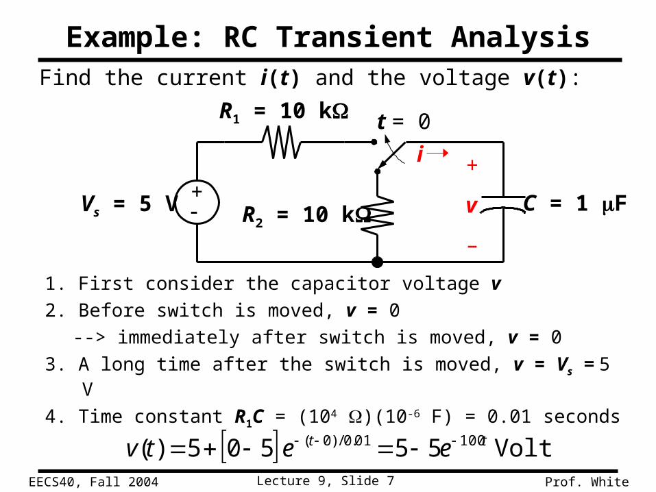
Example: RC Transient AnalysisFind the current i(t) and the voltage v(t):

t = 0

i +

v

–

R2 = 10 kVs = 5 V + C = 1 F

1. First consider the capacitor voltage v

2. Before switch is moved, v = 0

--> immediately after switch is moved, v = 0

3. A long time after the switch is moved, v = Vs = 5 V

4. Time constant R1C = (104 )(10-6 F) = 0.01 seconds

Volts 55 505)( 10001.0/)0( tt eetv

R1 = 10 k


t = 0

i +

v

–

R2 = 10 kVs = 5 V + C = 1 F

4

100

1 10

555)()(

ts e

R

tvVti

R1 = 10 k

Now solve for i(t), for t > 0:

From Ohm’s Law, A

= 5 x 10-4e-100t A




When we perform a sequence of computations using a digital circuit, we switch the input voltages between logic 0 (e.g., 0 Volts) and logic 1 (e.g., 5 Volts).

The output of the digital circuit changes between logic 0 and logic 1 as computations are performed.

Application to Digital Integrated Circuits (ICs)


• Every node in a real circuit has capacitance; it’s the charging of these capacitances that limits circuit performance (speed)

We compute with pulses.

We send beautiful pulses in:

But we receive lousy-looking pulses at the output:

Capacitor charging effects are responsible!

time

volt

age

time

volt

age

Digital Signals


Circuit Model for a Logic Gate

• Recall (from Lecture 1) that electronic building blocks referred to as “logic gates” are used to implement logical functions (NAND, NOR, NOT) in digital ICs– Any logical function can be implemented using these gates.

• A logic gate can be modeled as a simple RC circuit:

+

Vout

–

R

Vin(t) + C

switches between “low” (logic 0) and “high” (logic 1) voltage states


Transition from “0” to “1”

(capacitor charging)

time

Vout

0

Vhigh

RC

0.63Vhigh

Vout

Vhigh

timeRC

0.37Vhigh

Transition from “1” to “0”

(capacitor discharging)

(Vhigh is the logic 1 voltage level)

Logic Level Transitions

RCthighout eVtV /1)( RCt

highout eVtV /)(

0


What if we step up the input,

wait for the output to respond,

then bring the input back down?

time

Vin

0

0

time

Vin

0

0

Vout

time

Vin

0

0

Vout

Sequential Switching


The input voltage pulse width must be large enough; otherwise the output pulse is distorted.

(We need to wait for the output to reach a recognizable logic level, before changing the input again.)

0

1

2

3

4

5

6

0 1 2 3 4 5Time

Vo

ut

Pulse width = 0.1RC

01

23

45

6

0 1 2 3 4 5Time

Vo

ut

0

1

2

3

4

5

6

0 5 10 15 20 25Time

Vo

ut

Pulse Distortion

+

Vout

–

R

Vin(t) C+

–

Pulse width = 10RCPulse width = RC


Vin

RVout

C

Suppose a voltage pulse of width5 s and height 4 V is applied to theinput of this circuit beginning at t = 0:

R = 2.5 kΩC = 1 nF

• First, Vout will increase exponentially toward 4 V.

• When Vin goes back down, Vout will decrease exponentially back down to 0 V.

What is the peak value of Vout?

The output increases for 5 s, or 2 time constants.

It reaches 1-e-2 or 86% of the final value.

0.86 x 4 V = 3.44 V is the peak value

Example

= RC = 2.5 s


00.5

11.5

22.5

33.5

4

0 2 4 6 8 10

Vout(t) =4-4e-t/2.5s for 0 ≤ t ≤ 5 s

3.44e-(t-5s)/2.5s for t > 5 s{


Documents

Lecture 9, Slide 1EECS40, Fall 2004Prof. White Lecture #9 OUTLINE –Transient response of 1 st -order circuits –Application: modeling of digital logic gate