Lecture 9

Step-Index Optical Fibers (Lipson 10.3)

Of course, technologically the most important and familiar optical waveguide which confines light

in both x and y is the optical fiber. A common form of the fiber is a simple conceptual extension of

our slab guide:

2 1n n , of course

As usual, the propagation equation we have to solve (see p.A7) is the Helmholtz eqn.

2 2 2 0i oE n k E i=1,2

Now, given the symmetry of the problem, we need to work in cylindrical coordinates

ˆˆ ˆ( ) ( , , ) ( , , ) ( , , ) ( , , )r zE r E r z rE r z E r z zE r z

One subtle point (see Pollock Chapter 5.2) is that the rE and E components cannot be decoupled.

This can be illustrated schematically by the following example, where an initially purely radial

field becomes a mostly azimuthal field in propagation:

On the other hand, a purely z component of the field remain so

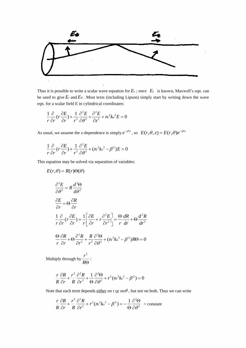
Thus it is possible to write a scalar wave equation for zE ; once zE is known, Maxwell’s eqn. can

be used to give rE and E . Most texts (including Lipson) simply start by writing down the wave

eqn. for a scalar field E in cylindrical coordinates:

2 2

2 2 2

2 21 1( ) 0i o

E E Er n k E

r r r r z

As usual, we assume the z-dependence is simplyi ze

, so ( , , ) ( , ) i zE r z E r e

2

2 2

2 2 21 1( ) ( ) 0i o

E Er n k E

r r r r

This equation may be solved via separation of variables:

( , ) ( ) ( )E r R r

2 2

2 2

E dR

d

E R

r r

2 2

2 2

1 1( )

E E E dR d Rr r

r r r r r r r dr dr

2 2

2 2 2

2 2 2( ) 0i oR R R

n k Rr r r r

Multiply through by

2r

R:

2 22

2 2

22 2 21

( ) 0i oR Rr r

r n kR Rr r

Note that each term depends either on r or on , but not on both. Thus we can write

2 22

2 2

22 2 2 1

( )i oR Rr r

r n kR Rr r

= constant

(both sides are independent, so they must equal a constant ).

By convention, the constant is called2l .

(1) Azimuthal eqn.

22

2

1l

22

20l

=> ( ) cos sinA l B l

(some texts write it as il ilAe Be )

Thus we find azimuthal modes, where the field is modulated angularly (i.e. in the intensity,

observe an even # of lobes)

(2) Radial Eqn:

2 2

2 2

2 2 21( ) 0i o

R R ln k R

rr r r

Just as with the slab waveguide, in order to have bound solutions, we must have

2

o

n k in the core

1

o

n k in the cladding

define 2 2 2 2

2

on k ( =”kappa”)

2 2 2 2

1

on k

=> we have radial eqn., for the core and cladding

(i) core :

2 22

2 2

1( ) 0

R R lR

rr r r

(ii) cladding:

2 22

2 2

1( ) 0

R R lR

rr r r

The solutions to these equations are the family of Bessel functions. They share some

common features with the sine, cosine, and experimental solutions we found appropriate for

the slab waveguide problem.

(1) As usual, we ignore mathematical solutions which diverge as 0r or

as r , since these are unphysical!

(2) In Eqn.(i), when

22

20

l

r , the solution is the Bessel function of the first kind of

order l, usually written ( )lJ r

Two things to remember:

(a) The lJ functions are oscillatory functions of r, just like sines and cosines. (see plot

Figure 5.4)

In fact, when 1r (large r), they are simply damped cosines:

12

( ) c o s , 12 2

lJ r r l rr

(b) The Bessel functions are orthogonal, just as the sine and cosine modes of the slab

problem.

(3) In eqn. (ii), when

22

20

l

r , the solution is the Bessel function of the second kind of

order l, usually written ( )l r .

The l are damped solutions. In fact, when 1 r ,

( )2

l

re

rr

Note that higher-order modes (l>0) will both radial and angular modulation.

As with the slab waveguide, the allowed values of (i.e. the eigenvalues) of the

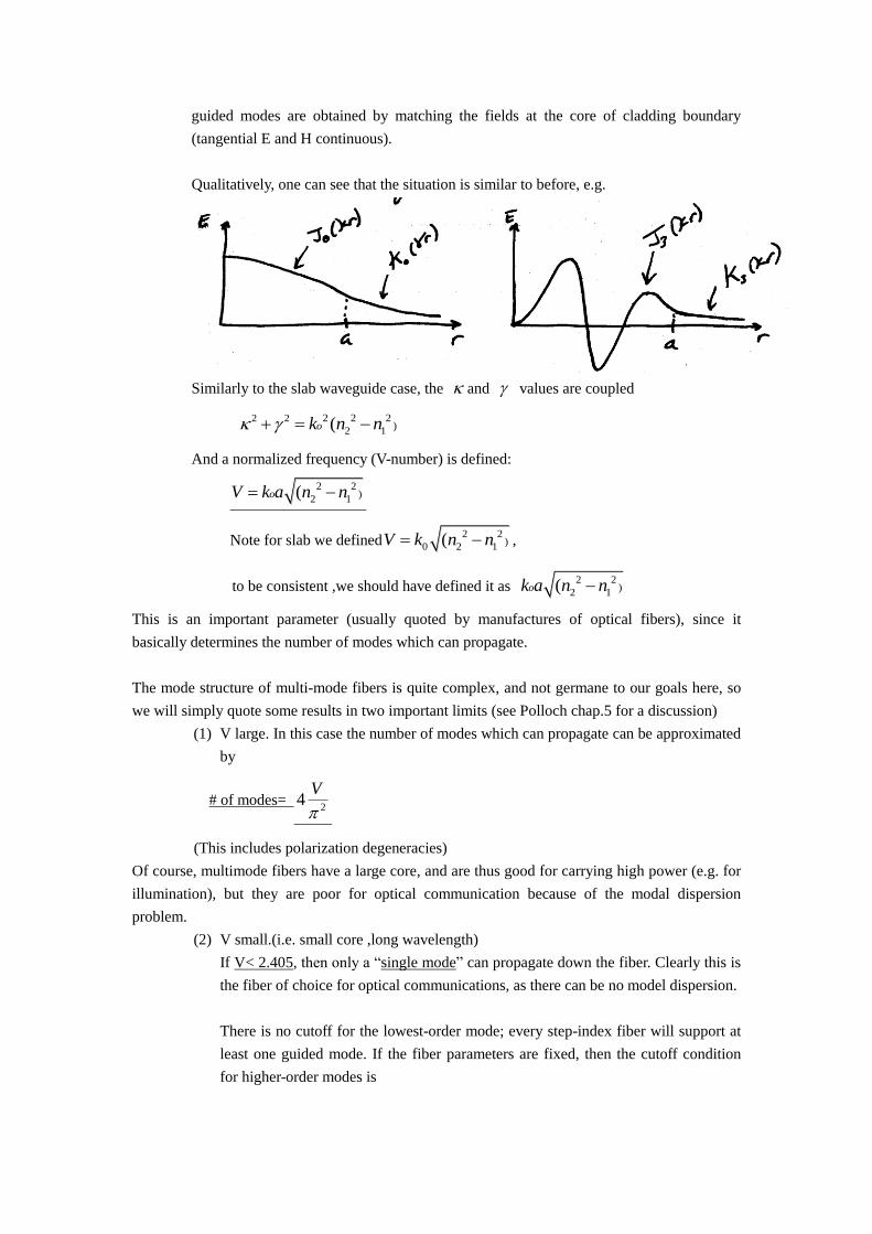
guided modes are obtained by matching the fields at the core of cladding boundary

(tangential E and H continuous).

Qualitatively, one can see that the situation is similar to before, e.g.

Similarly to the slab waveguide case, the and values are coupled

2 2 2 2 2

)2 1

( ok n n

And a normalized frequency (V-number) is defined:

2 2

)2 1

( oV k a n n

Note for slab we defined2 2

)0 2 1

( V k n n ,

to be consistent ,we should have defined it as 2 2

)2 1

( ok a n n

This is an important parameter (usually quoted by manufactures of optical fibers), since it

basically determines the number of modes which can propagate.

The mode structure of multi-mode fibers is quite complex, and not germane to our goals here, so

we will simply quote some results in two important limits (see Polloch chap.5 for a discussion)

(1) V large. In this case the number of modes which can propagate can be approximated

by

# of modes= 2

4

V

(This includes polarization degeneracies)

Of course, multimode fibers have a large core, and are thus good for carrying high power (e.g. for

illumination), but they are poor for optical communication because of the modal dispersion

problem.

(2) V small.(i.e. small core ,long wavelength)

If V< 2.405, then only a “single mode” can propagate down the fiber. Clearly this is

the fiber of choice for optical communications, as there can be no model dispersion.

There is no cutoff for the lowest-order mode; every step-index fiber will support at

least one guided mode. If the fiber parameters are fixed, then the cutoff condition

for higher-order modes is

2 2

2 1

2( )

2.405

c

an n

Now, it should be noted that the term “single-mode fiber” is a little bit of a misnomer. The fiber is

cylindrically symmetric, so it cannot distinguish input polarizations. In other words, we could

inject wave polarized either along x or along y , and they both would have the same mode

profile and the same . (These two modes are “degenerate”)

The functional form of the field profile of the fundamental mode in the core is the 0J Bessel

function.

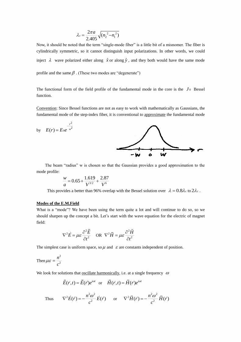
Convention: Since Bessel functions are not as easy to work with mathematically as Gaussians, the

fundamental mode of the step-index fiber, it is conventional to approximate the fundamental mode

by

2

20( )

r

wE r E e

The beam “radius” w is chosen so that the Gaussian provides a good approximation to the

mode profile:

3/2 6

1.619 2.870.65

w

a V V

This provides a better than 96% overlap with the Bessel solution over 0.8 c to 2 c .

Modes of the E.M.Field

What is a “mode”? We have been using the term quite a lot and will continue to do so, so we

should sharpen up the concept a bit. Let’s start with the wave equation for the electric of magnet

field:

22

2

EE

t

OR

22

2

HH

t

The simplest case is uniform space, so and are constants independent of position.

Then

2

2

n

c

We look for solutions that oscillate harmonically, i.e. at a single frequency

( , ) ( ) i tE r t E r e or ( , ) ( ) i tH r t H r e

Thus

2 22

2( ) ( )

nE r E r

c

or

2 22

2( ) ( )

nH r H r

c

We usually define the wavevector n

kc

, so we have the Helmholtz equations

2 2( ) ( )E r k E r or

2 2( ) ( )H r k H r

2 : operator;

2k : constant = eigenvalue

These are eigenvalue equations.

That is, when a functional operator (2 in this case) acts on an eigenfunction (a “mode”), it

yields the same spatial function (the mode) multiplied by a constant (the eigenvalue).

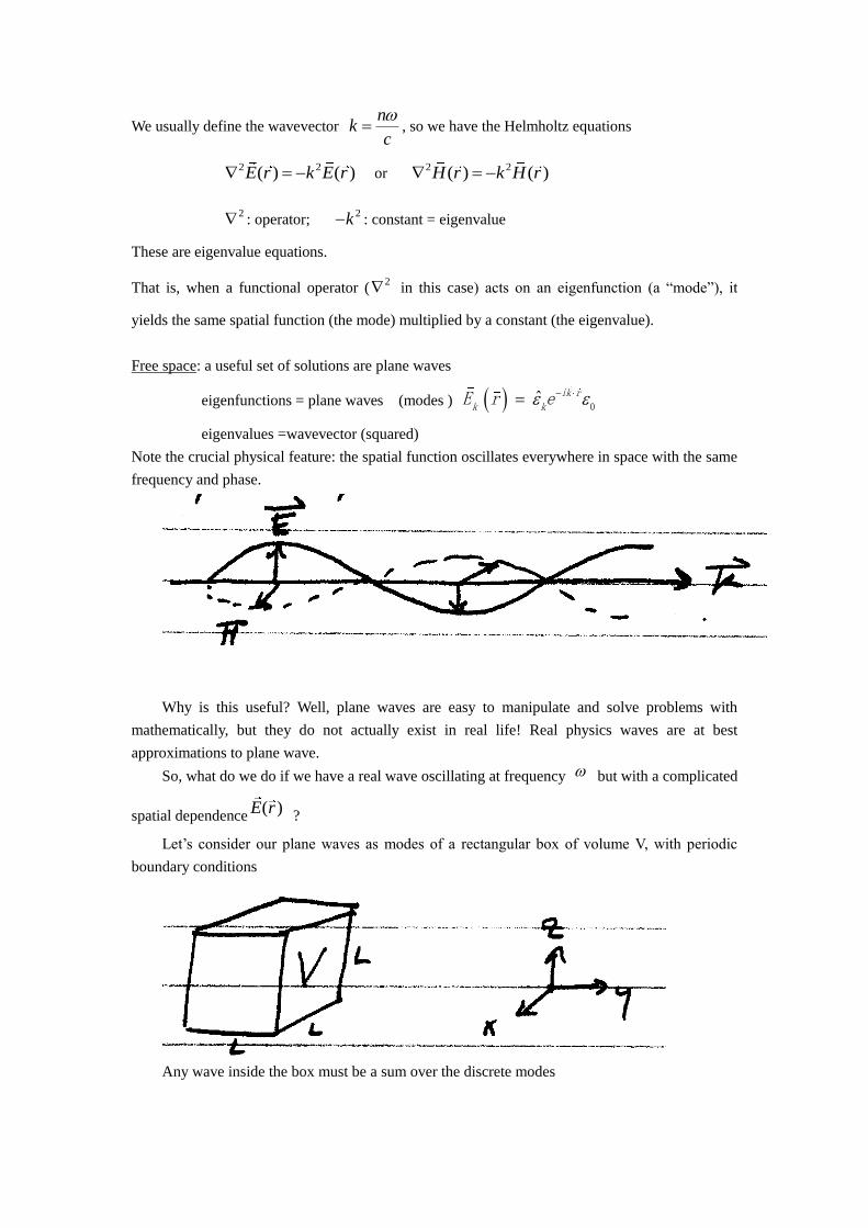
Free space: a useful set of solutions are plane waves

eigenfunctions = plane waves (modes ) 0ˆ ik r

k kE r e

eigenvalues =wavevector (squared)

Note the crucial physical feature: the spatial function oscillates everywhere in space with the same

frequency and phase.

Why is this useful? Well, plane waves are easy to manipulate and solve problems with

mathematically, but they do not actually exist in real life! Real physics waves are at best

approximations to plane wave.

So, what do we do if we have a real wave oscillating at frequency but with a complicated

spatial dependence( )E r

?

Let’s consider our plane waves as modes of a rectangular box of volume V, with periodic

boundary conditions

Any wave inside the box must be a sum over the discrete modes

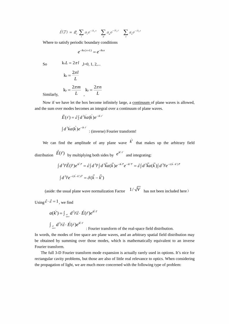
( ) ?( )( )( ) yx zik yik x ik z

r i m ni m n

E r a e a e a e

Where to satisfy periodic boundary conditions

x xk ( ) ki x L i xe e

So k 2xL l ,l=0, 1, 2,...

2kx

l

L

Similarly,

2ky

m

L

,

2kz

n

L

Now if we have let the box become infinitely large, a continuum of plane waves is allowed,

and the sum over modes becomes an integral over a continuum of plane waves.

3ˆ( ) ( ) ik rE r d ka k e

3 ( ) ik rd ka k e

: (inverse) Fourier transform!

We can find the amplitude of any plane wave k that makes up the arbitrary field

distribution ( )E r

by multiplying both sides by ik re

and integrating:

(3 3 3 3 3 )ˆ ˆ( ) ( ) ( )i i i ik r k r k r k k rd rE r e d r d ka k e e d ka k d re

(3 ) ( )i k k rd re k k

(aside: the usual plane wave normalization Factor 1/ V has not been included here）

Using ˆ ˆ 1 , we find

3 ˆ( ) ( )all

space

ik ra k d r E r e

3 ˆ ( )all

space

ik rd r E r e : Fourier transform of the real-space field distribution.

In words, the modes of free space are plane waves, and an arbitrary spatial field distribution may

be obtained by summing over those modes, which is mathematically equivalent to an inverse

Fourier transform.

The full 3-D Fourier transform mode expansion is actually rarely used in options. It’s nice for

rectangular cavity problems, but those are also of little real relevance to optics. When considering

the propagation of light, we are much more concerned with the following type of problem:

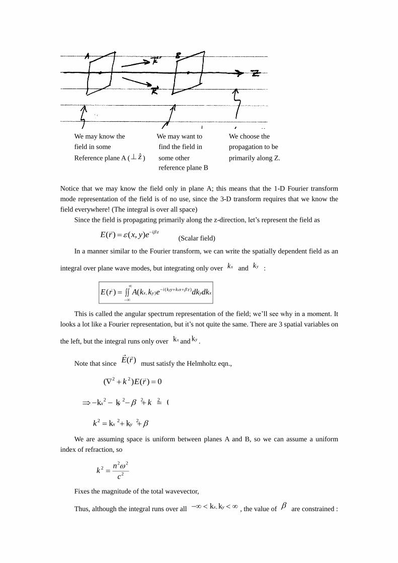
We may know the We may want to We choose the

field in some find the field in propagation to be

Reference plane A ( z ) some other primarily along Z.

reference plane B

Notice that we may know the field only in plane A; this means that the 1-D Fourier transform

mode representation of the field is of no use, since the 3-D transform requires that we know the

field everywhere! (The integral is over all space)

Since the field is propagating primarily along the z-direction, let’s represent the field as

( ) ( , ) i zE r x y e

(Scalar field)

In a manner similar to the Fourier transform, we can write the spatially dependent field as an

integral over plane wave modes, but integrating only over xk and yk :

( ), )( ) ( y xi k y k x z

x y y xE r A k k e dk dk

This is called the angular spectrum representation of the field; we’ll see why in a moment. It

looks a lot like a Fourier representation, but it’s not quite the same. There are 3 spatial variables on

the left, but the integral runs only over kx and ky .

Note that since ( )E r

must satisfy the Helmholtz eqn.,

2 2( ) ( ) 0k E r

2 2 2 2k k 0x y k

2 2 2 2k kx yk

We are assuming space is uniform between planes A and B, so we can assume a uniform

index of refraction, so

2 22

2

nk

c

Fixes the magnitude of the total wavevector,

Thus, although the integral runs over all ,k kx y , the value of

are constrained :

2 22 2 2

2k kx y

n

c

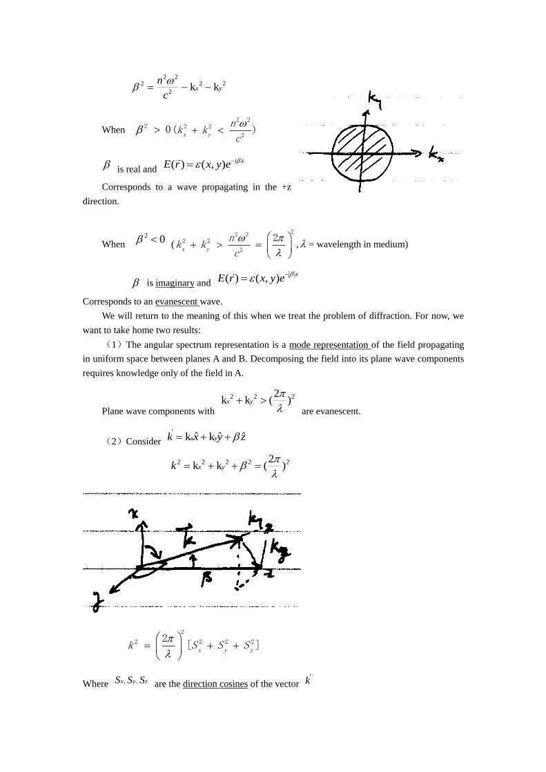
When 2 0

2 22 2

2( )x y

nk k

c

is real and ( ) ( , ) i zE r x y e

Corresponds to a wave propagating in the +z

direction.

When 2 0

(

22 22 2

2

2x y

nk k

c

, = wavelength in medium)

is imaginary and ( ) ( , )z

E r x y e

Corresponds to an evanescent wave.

We will return to the meaning of this when we treat the problem of diffraction. For now, we

want to take home two results:

（1）The angular spectrum representation is a mode representation of the field propagating

in uniform space between planes A and B. Decomposing the field into its plane wave components

requires knowledge only of the field in A.

Plane wave components with

2 2 22k k ( )x y

are evanescent.

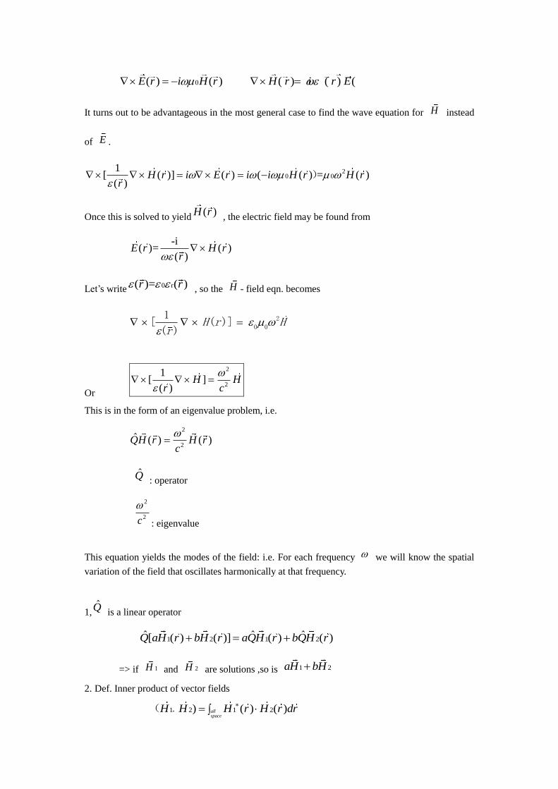
（2）Consider ˆ ˆ ˆk kx yk x y z

2 2 2 2 22k k ( )x yk

2

2 2 2 22[ ]x y z

k S S S

Where , ,x y zS S S are the direction cosines of the vector k

i.e. cos i

i

kS

k

, i = x , y , z

S = unit vector in direction of propagation:

2 ˆk S

And 2 2 2ˆ ˆ 1( 1)x y zS S S S S

Thus the decomposition of a field into its angular spectrum corresponds to decomposing it into

plane wave modes propagating at different angles with respect to the z axis.

Supplementary

Generalized mode problem

So far we have treated the problem of finding the modes of free space, or of specific geometrics

such as the slab waveguide or cylindrical fiber. It is interesting to consider the properties of modes

in general, where the dielectric constant may be a function of position.

E.g. Multilayer mirror

E.g. Photonic crystal

We follow the treatment of Joannopoulos, Mender, and Winn, Photonic Crystals, chap .2.

As usual, we begin with the source-free Maxwell eqns.

0D 0B

E -

B

t

DH

t

With constitutive relation

( , ) ( ) ( , )D r r E r

0 ( 1 )rB H

We are looking for modes, which oscillate at an angle frequency :

( , ) ( ) i tE r t E r e

( , ) ( )i tH r t H r e

So [ ( ) ( )] 0r E r

( ) 0H r

0( ) ( )E r i H r

( ) ( ) ( )H r i r E r

It turns out to be advantageous in the most general case to find the wave equation for H instead

of E .

20 0

1[ ( )] ( ) ( ( ) = ( )

( )H r i E r i i H r H r

r

）

Once this is solved to yield( )H r

, the electric field may be found from

-i( )= ( )

( )E r H r

r

Let’s write 0 r( )= ( )r r , so the H - field eqn. becomes

2

0 0

1[ ( )]( )

H r Hr

Or

2

2

1[ ]

( )H H

r c

This is in the form of an eigenvalue problem, i.e.

2

2ˆ ( ) ( )QH r H r

c

Q : operator

2

2c

: eigenvalue

This equation yields the modes of the field: i.e. For each frequency we will know the spatial

variation of the field that oscillates harmonically at that frequency.

1,Q is a linear operator

1 2 1 2ˆ ˆ ˆ[ ( ) ( )] ( ) ( )Q aH r bH r aQH r bQH r

=> if 1H and 2H are solutions ,so is 1 2aH bH

2. Def. Inner product of vector fields

1 2 1 2) ( ) ( )all

space

H H H r H r dr ，（

Two vector fields are orthogonal if 1 2) 0H H ，（

Normalization : a vector field H is normalized if ) 1H H ，（

If ) 1H H ，（

, then can always normalize by

( )

)

H rF

H H

（ ， , so

( , ) 1F F (proof trivial).

3. Q is a Hermitian operator , i.e. 1 2 1, 2ˆ ˆ) ( )H QH QH H，（

Pf.

3 3 31 2 1 2 1 2 1 2 1, 2

1 1 1ˆ ˆ) ( )rr r

H QH d rH H d r H H d r H H QH H

，（

(details: homework #2 )

4. Q is Hermitian => eigenvalue

2

c

is always real and positive (the latter requires the

assumption 0r everywhere ). Proof is left as an exercise to the readers,

5 . Q is Hermitian => two modes with different frequencies 1 , 2 are orthogonal ( this is the

most important result of this section ).

Pf. Suppose 1 2

1 1 2 2( , ) ( ) , ( , ) ( )i t i tH r t H r e H r t H r e with 1 2,H H being normalized

modes (eigenfunction ).

2 2

2 2

1 12 1 2 1 2 1) ) ( , )H QH H H H H

c c

， ，（ （

2

2

22 1 2 1 2 1ˆ) ( , ) ( , )H QH QH H H H

c

，（

Subtract : 2 2

2 1 2 1( )( , ) 0H H

=> if 2 1 , then 2 1( , ) 0H H

What if 2 1 ? (In this case, the modes are said to be “degenerate”)

An example would be two plane waves with the same frequency but propagating in different

directions:

1 21 2 1 2, ,ik r ik r n

H e H e k kc

2 1)(3

1 2 2 1( , ) ( ) 0i k k rH H d re k k if 2 1k k

Fact (quoted without proof here): since Q is linear , one can always construct linear

combinations of modes which are mutually orthogonal , so one can always construct orthonormal

sets of eigenmodes sets of eigenmodes for degenerate as well as nondegenerate modes .

(Technique: Schmidt orthogonalization )

6.The modes found by solving the eigenvalue problem form a complete set .Thus any possible

electromagnetic field can be written as a sum over eigenmodes :

3( ) ( ) ( ) ( )qq

qH r a H r a q H q d q

( )qq

qa H r Appropriate for discrete modes

3( ) ( )a q H q d q continuum modes ( q may be k , or some other variable

characterize the eigenmodes )