Lecture 5: Model-Free Control - Chonbuknlp.chonbuk.ac.kr/AML/slides_silva/control.pdf · Lecture 5: Model-Free Control Lecture 5: Model-Free Control David Silver. Lecture 5: Model-Free

Lecture 5: Model-Free Control


David Silver


Outline

1 Introduction

2 On-Policy Monte-Carlo Control

3 On-Policy Temporal-Difference Learning

4 Off-Policy Learning

5 Summary


Introduction

Model-Free Reinforcement Learning

Last lecture:

Model-free predictionEstimate the value function of an unknown MDP

This lecture:

Model-free controlOptimise the value function of an unknown MDP


Introduction

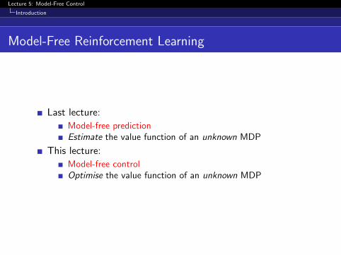
Uses of Model-Free Control

Some example problems that can be modelled as MDPs

Elevator

Parallel Parking

Ship Steering

Bioreactor

Helicopter

Aeroplane Logistics

Robocup Soccer

Quake

Portfolio management

Protein Folding

Robot walking

Game of Go

For most of these problems, either:

MDP model is unknown, but experience can be sampled

MDP model is known, but is too big to use, except by samples

Model-free control can solve these problems


Introduction

On and Off-Policy Learning

On-policy learning

“Learn on the job”Learn about policy π from experience sampled from π

Off-policy learning

“Look over someone’s shoulder”Learn about policy π from experience sampled from µ


On-Policy Monte-Carlo Control

Generalised Policy Iteration

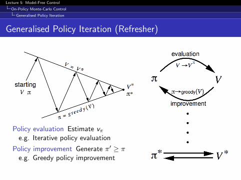
Generalised Policy Iteration (Refresher)

Policy evaluation Estimate vπe.g. Iterative policy evaluation

Policy improvement Generate π′ ≥ πe.g. Greedy policy improvement




Generalised Policy Iteration With Monte-Carlo Evaluation

Policy evaluation Monte-Carlo policy evaluation, V = vπ?

Policy improvement Greedy policy improvement?




Model-Free Policy Iteration Using Action-Value Function

Greedy policy improvement over V (s) requires model of MDP

π′(s) = argmaxa∈A

Ras + Pa

ss′V (s ′)

Greedy policy improvement over Q(s, a) is model-free

π′(s) = argmaxa∈A

Q(s, a)




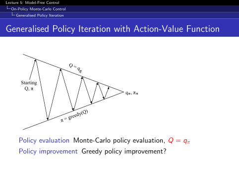
Generalised Policy Iteration with Action-Value Function

Starting Q, π

π = greedy(Q)

Q = qπ

q*, π*

Policy evaluation Monte-Carlo policy evaluation, Q = qπ

Policy improvement Greedy policy improvement?



Exploration

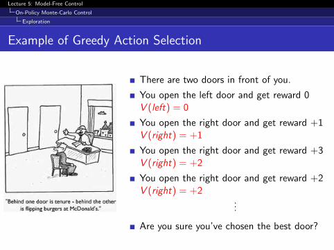
Example of Greedy Action Selection

There are two doors in front of you.

You open the left door and get reward 0V (left) = 0

You open the right door and get reward +1V (right) = +1



...

Are you sure you’ve chosen the best door?



Exploration

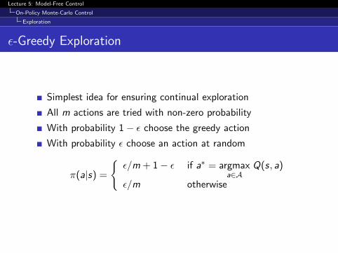
ε-Greedy Exploration

Simplest idea for ensuring continual exploration

All m actions are tried with non-zero probability

With probability 1− ε choose the greedy action

With probability ε choose an action at random

π(a|s) =

{ε/m + 1− ε if a∗ = argmax

a∈AQ(s, a)

ε/m otherwise



Exploration

ε-Greedy Policy Improvement

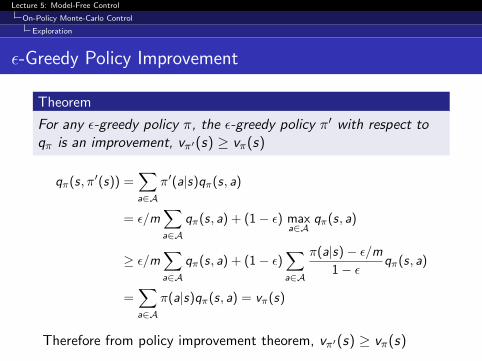
Theorem

For any ε-greedy policy π, the ε-greedy policy π′ with respect toqπ is an improvement, vπ′(s) ≥ vπ(s)

qπ(s, π′(s)) =∑a∈A

π′(a|s)qπ(s, a)

= ε/m∑a∈A

qπ(s, a) + (1− ε) maxa∈A

qπ(s, a)

≥ ε/m∑a∈A

qπ(s, a) + (1− ε)∑a∈A

π(a|s)− ε/m1− ε qπ(s, a)

=∑a∈A

π(a|s)qπ(s, a) = vπ(s)

Therefore from policy improvement theorem, vπ′(s) ≥ vπ(s)



Exploration

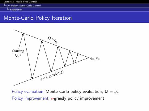
Monte-Carlo Policy Iteration

Starting Q, π

π = ε-greedy(Q)

Q = qπ

q*, π*

Policy evaluation Monte-Carlo policy evaluation, Q = qπ

Policy improvement ε-greedy policy improvement



Exploration

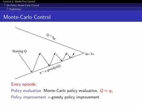
Monte-Carlo Control

Starting Q

π = ε-greedy(Q)

Q = qπ

q*, π*

Every episode:

Policy evaluation Monte-Carlo policy evaluation, Q ≈ qπ




GLIE

GLIE

Definition

Greedy in the Limit with Infinite Exploration (GLIE)

All state-action pairs are explored infinitely many times,

limk→∞

Nk(s, a) =∞

The policy converges on a greedy policy,

limk→∞

πk(a|s) = 1(a = argmaxa′∈A

Qk(s, a′))

For example, ε-greedy is GLIE if ε reduces to zero at εk = 1k



GLIE

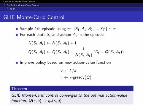
GLIE Monte-Carlo Control

Sample kth episode using π: {S1,A1,R2, ...,ST} ∼ πFor each state St and action At in the episode,

N(St ,At)← N(St ,At) + 1

Q(St ,At)← Q(St ,At) +1

N(St ,At)(Gt − Q(St ,At))

Improve policy based on new action-value function

ε← 1/k

π ← ε-greedy(Q)

Theorem

GLIE Monte-Carlo control converges to the optimal action-valuefunction, Q(s, a)→ q∗(s, a)



Blackjack Example

Back to the Blackjack Example



Blackjack Example

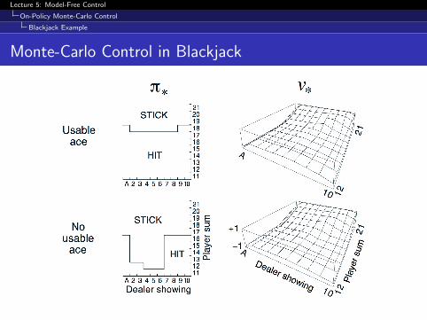
Monte-Carlo Control in Blackjack


On-Policy Temporal-Difference Learning

MC vs. TD Control

Temporal-difference (TD) learning has several advantagesover Monte-Carlo (MC)

Lower varianceOnlineIncomplete sequences

Natural idea: use TD instead of MC in our control loop

Apply TD to Q(S ,A)Use ε-greedy policy improvementUpdate every time-step



Sarsa(λ)

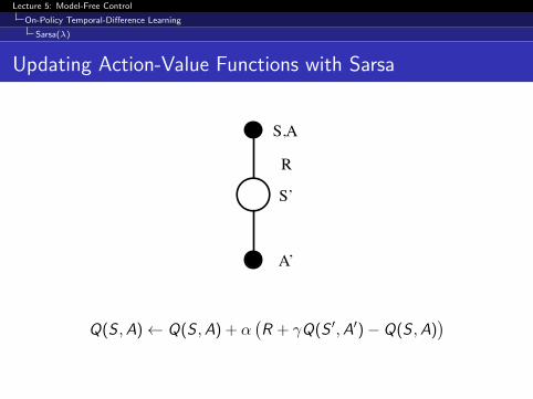
Updating Action-Value Functions with Sarsa

S,A

R

A’

S’

Q(S ,A)← Q(S ,A) + α(R + γQ(S ′,A′)− Q(S ,A)

)



Sarsa(λ)

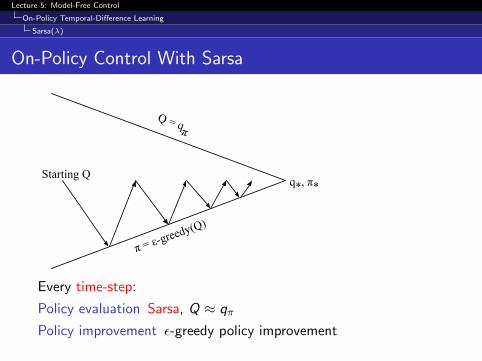
On-Policy Control With Sarsa

Starting Q

π = ε-greedy(Q)

Q = qπ

q*, π*

Every time-step:

Policy evaluation Sarsa, Q ≈ qπ




Sarsa(λ)

Sarsa Algorithm for On-Policy Control



Sarsa(λ)

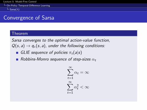
Convergence of Sarsa

Theorem

Sarsa converges to the optimal action-value function,Q(s, a)→ q∗(s, a), under the following conditions:

GLIE sequence of policies πt(a|s)

Robbins-Monro sequence of step-sizes αt

∞∑t=1

αt =∞

∞∑t=1

α2t <∞



Sarsa(λ)

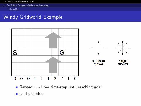
Windy Gridworld Example

Reward = -1 per time-step until reaching goal

Undiscounted



Sarsa(λ)

Sarsa on the Windy Gridworld



Sarsa(λ)

n-Step Sarsa

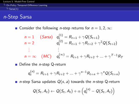
Consider the following n-step returns for n = 1, 2,∞:

n = 1 (Sarsa) q(1)t = Rt+1 + γQ(St+1)

n = 2 q(2)t = Rt+1 + γRt+2 + γ2Q(St+2)

......

n =∞ (MC ) q(∞)t = Rt+1 + γRt+2 + ...+ γT−1RT

Define the n-step Q-return

q(n)t = Rt+1 + γRt+2 + ...+ γn−1Rt+n + γnQ(St+n)

n-step Sarsa updates Q(s, a) towards the n-step Q-return

Q(St ,At)← Q(St ,At) + α(q

(n)t − Q(St ,At)

)



Sarsa(λ)

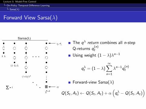
Forward View Sarsa(λ)

The qλ return combines all n-step

Q-returns q(n)t

Using weight (1− λ)λn−1

qλt = (1− λ)∞∑n=1

λn−1q(n)t

Forward-view Sarsa(λ)

Q(St ,At)← Q(St ,At) + α(qλt − Q(St ,At)

)



Sarsa(λ)

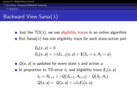
Backward View Sarsa(λ)

Just like TD(λ), we use eligibility traces in an online algorithm

But Sarsa(λ) has one eligibility trace for each state-action pair

E0(s, a) = 0

Et(s, a) = γλEt−1(s, a) + 1(St = s,At = a)

Q(s, a) is updated for every state s and action a

In proportion to TD-error δt and eligibility trace Et(s, a)

δt = Rt+1 + γQ(St+1,At+1)− Q(St ,At)

Q(s, a)← Q(s, a) + αδtEt(s, a)



Sarsa(λ)

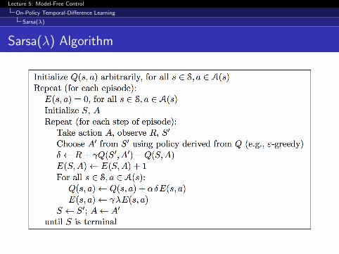
Sarsa(λ) Algorithm



Sarsa(λ)

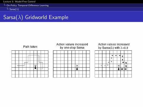
Sarsa(λ) Gridworld Example


Off-Policy Learning

Off-Policy Learning

Evaluate target policy π(a|s) to compute vπ(s) or qπ(s, a)

While following behaviour policy µ(a|s)

{S1,A1,R2, ...,ST} ∼ µ

Why is this important?

Learn from observing humans or other agents

Re-use experience generated from old policies π1, π2, ..., πt−1

Learn about optimal policy while following exploratory policy

Learn about multiple policies while following one policy


Off-Policy Learning

Importance Sampling

Importance Sampling

Estimate the expectation of a different distribution

EX∼P [f (X )] =∑

P(X )f (X )

=∑

Q(X )P(X )

Q(X )f (X )

= EX∼Q

[P(X )

Q(X )f (X )

]


Off-Policy Learning

Importance Sampling

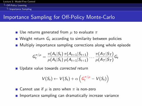
Importance Sampling for Off-Policy Monte-Carlo

Use returns generated from µ to evaluate π

Weight return Gt according to similarity between policies

Multiply importance sampling corrections along whole episode

Gπ/µt =

π(At |St)µ(At |St)

π(At+1|St+1)

µ(At+1|St+1). . .

π(AT |ST )

µ(AT |ST )Gt

Update value towards corrected return

V (St)← V (St) + α(Gπ/µt − V (St)

)Cannot use if µ is zero when π is non-zero

Importance sampling can dramatically increase variance


Off-Policy Learning

Importance Sampling

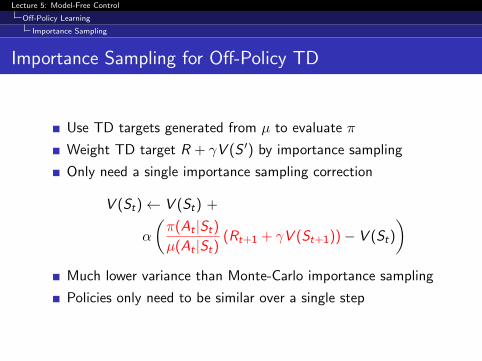
Importance Sampling for Off-Policy TD

Use TD targets generated from µ to evaluate π

Weight TD target R + γV (S ′) by importance sampling

Only need a single importance sampling correction

V (St)← V (St) +

α

(π(At |St)µ(At |St)

(Rt+1 + γV (St+1))− V (St)

)Much lower variance than Monte-Carlo importance sampling

Policies only need to be similar over a single step


Off-Policy Learning

Q-Learning

Q-Learning

We now consider off-policy learning of action-values Q(s, a)

No importance sampling is required

Next action is chosen using behaviour policy At+1 ∼ µ(·|St)But we consider alternative successor action A′ ∼ π(·|St)And update Q(St ,At) towards value of alternative action

Q(St ,At)← Q(St ,At) + α(Rt+1 + γQ(St+1,A

′)− Q(St ,At))


Off-Policy Learning

Q-Learning

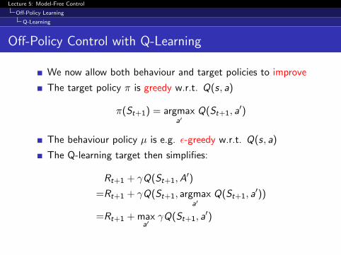
Off-Policy Control with Q-Learning

We now allow both behaviour and target policies to improve

The target policy π is greedy w.r.t. Q(s, a)

π(St+1) = argmaxa′

Q(St+1, a′)

The behaviour policy µ is e.g. ε-greedy w.r.t. Q(s, a)

The Q-learning target then simplifies:

Rt+1 + γQ(St+1,A′)

=Rt+1 + γQ(St+1, argmaxa′

Q(St+1, a′))

=Rt+1 + maxa′

γQ(St+1, a′)


Off-Policy Learning

Q-Learning

Q-Learning Control Algorithm

S,A

R

A’

S’

Q(S ,A)← Q(S ,A) + α

(R + γ max

a′Q(S ′, a′)− Q(S ,A)

)

Theorem

Q-learning control converges to the optimal action-value function,Q(s, a)→ q∗(s, a)


Off-Policy Learning

Q-Learning

Q-Learning Algorithm for Off-Policy Control


Off-Policy Learning

Q-Learning

Q-Learning Demo

Q-Learning Demo

''http://www.cs.ubc.ca/~poole/demos/rl/q.html''


Off-Policy Learning

Q-Learning

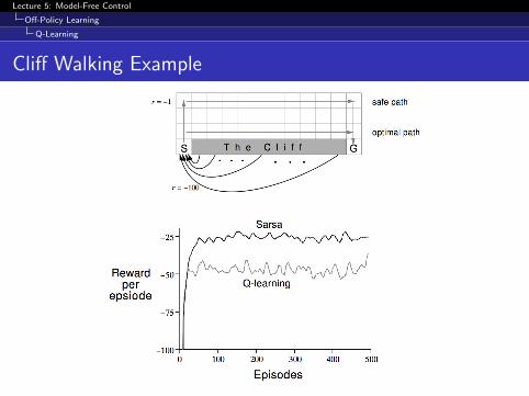
Cliff Walking Example


Summary

Relationship Between DP and TD

Full Backup (DP) Sample Backup (TD)

Bellman Expectation v⇡(s0) 7!s0

v⇡(s) 7!s

r

a

Equation for vπ(s) Iterative Policy Evaluation TD Learning

Bellman Expectation

q⇡(s, a) 7!s, a

q⇡(s0, a0) 7!a0

r

s0

S,A

R

A’

S’

Equation for qπ(s, a) Q-Policy Iteration Sarsa

Bellman Optimality q⇤(s0, a0) 7!a0

r

q⇤(s, a) 7!s, a

s0

Equation for q∗(s, a) Q-Value Iteration Q-Learning


Summary

Relationship Between DP and TD (2)

Full Backup (DP) Sample Backup (TD)

Iterative Policy Evaluation TD Learning

V (s)← E [R + γV (S ′) | s] V (S)α← R + γV (S ′)

Q-Policy Iteration Sarsa

Q(s, a)← E [R + γQ(S ′,A′) | s, a] Q(S ,A)α← R + γQ(S ′,A′)

Q-Value Iteration Q-Learning

Q(s, a)← E[R + γ max

a′∈AQ(S ′, a′) | s, a

]Q(S ,A)

α← R + γ maxa′∈A

Q(S ′, a′)

where xα← y ≡ x ← x + α(y − x)


Summary

Questions?

Documents

Lecture 5: Model-Free Control - Chonbuknlp.chonbuk.ac.kr/AML/slides_silva/control.pdf · Lecture 5: Model-Free Control Lecture 5: Model-Free Control David Silver. Lecture 5: Model-Free