Solid State Physics

FREE ELECTRON MODELLecture 14

A.H. HarkerPhysics and Astronomy

UCL

6 The Free Electron Model

6.1 Basic Assumptions

In the free electron model, we assume that the valence electrons canbe treated as free, or at least moving in a region constant potential,and non-interacting. We’ll examine the assumption of a constant po-tential first, and try to justify the neglect of interactions later.

2

6.1.1 Constant Potential

Imagine stripping the valence electrons from the atoms, and arrang-ing the resulting ion cores on the aatomic positions in the crystal.

Resulting potential – periodic array of Coulombic attractions.

3

From atomic theory, we are used to the idea that different electronicfunctions must be orthogonal to each other (remember we used thisidea in discussing the short-range repulsive part of interatomic po-tentials) i.e. if ψc(r) is a core function andψv(r) is a valence function∫

ψc(r)ψv(r)dr = 0.

Let’s see how orthogonality might be achieved for a slowly-varyingwave.

4

To achieve orthogonality:

we need high spatial frequency (largek) components in the wave.Large k → large energy.

5

So the extra energy caused by the orthogonality partly cancels theCoulomb potential. This can be formalised inpseudopotential theory.The potential is weakened,

and the constant potential assumption is a reasonable one. The netresult is that the effective potential seen by the electrons does nothave very strong dependence on position.

6

7

So finally we assume that the attractive potential of the ion cores canbe represented by a flat-bottomed potential.

We go further, and assume that the potential is deep enough that wecan use a simple ‘particle-in-a-box’ model – the free electron model.

8

6.1.2 Free Electron Fermi Gas

For the particle in a box with potential V

− ~2

2m∇2ψ + Vψ = E′ψ,

or, with a shift of origin for energy, E′ − V → E,

− ~2

2m∇2ψ = Eψ,

so that the wavefunctions have the form

ψk(r) =1√V

exp(ik.r),

where V is the volume of the material. These are travelling waves,with energies

Ek =~2k2

2m,

dependent only onk = |k|. Note thatEk depends only on themagni-tudeof k, not its direction.

9

So we can use the result from section 4.4 (Lecture 10) that the numberof states with modulus of wavevector betweenk and k + dk is

g(k)dk =V

8π34πk2dk =

V

2π2k2dk.

For electrons

dE

dk=

~2k

m=

~2

m

√2mE

~2=

~√m

√2E.

We also need to include a factor of 2 for spin up and spin down.

g(E) = 2g(k)dk

dE

= 2V

2π2k2 dk

dE

= 2V

2π2

2mE

~2

√m

~√

2E

=V m

π2~3

√2mE.

Note that asV increases, so does the density of states.

10

6.1.3 The Fermi Energy

Remember that the Fermi distribution function n(E)

n(E) =1

exp((E − EF )/kBT ) + 1at absolute zero is 1 up to the Fermi energyEF. Suppose the volumeV containsNe electrons. Then we know

Ne =

∫ ∞

0g(E)n(E)dE

=

∫ EF

0g(E)dE

=V√

2m3

π2~3

∫ EF

0

√E dE

=V√

2m3

π2~3

2EF3/2

3so

EF =~2

2m

(3π2NeV

)2/3

.

11

We can define two related quantities:

• Fermi temperature, TF,

TF = EF/kB.

• Fermi wavevector,kF, the magnitude of the wavevector correspond-ing to kF,

EF =~2kF

2

2mso

kF =

(3π2NeV

)1/3

.

12

6.1.4 Orders of magnitude

For a typical solid, the interatomic spacing is about2.5 × 10−10 m.Assume each atom is in a cube with that dimension, and releases onevalence electron, giving an electron densityNe/V ≈ 6 × 1028 m−3.Putting in the numbers, we find

• EF ≈ 9× 10−19 J = 6 eV;

• TF ≈ 70, 000 K;

• kF ≈ 1.2×1010 m−1, comparable with the reciprocal lattice spacing2.5× 1010 m−1;

We can also estimate the electron velocity at the Fermi energy:

vF =~kF

m≈ 1.4× 106m s−1,

which is fast, but not relativistic.

total energy of electrons =

∫ EF

0E g(E) dE =

3

5NeEF,

so that the average energy per electron is35EF.13

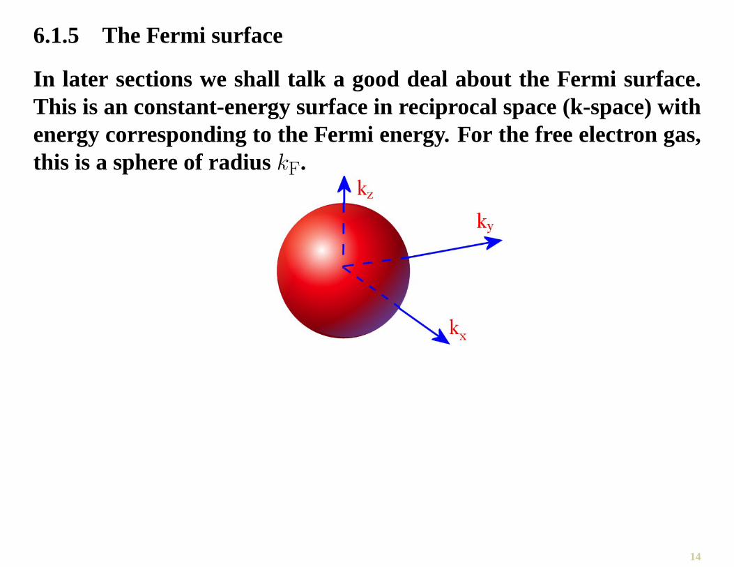
6.1.5 The Fermi surface

In later sections we shall talk a good deal about the Fermi surface.This is an constant-energy surface in reciprocal space (k-space) withenergy corresponding to the Fermi energy. For the free electron gas,this is a sphere of radiuskF.

14

6.2 Some simple properties of the free electron gas

6.2.1 Thermionic emission

If the work function φ is small enough, if the material is heated theelectrons may acquire enough thermal energy to escape the metal. Asmall electric field is used to draw them away.

15

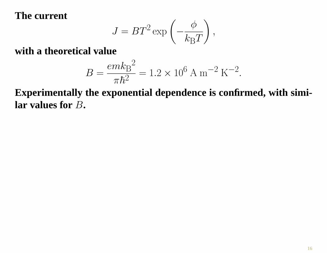
The current

J = BT 2 exp

(− φ

kBT

),

with a theoretical value

B =emkB

2

π~2= 1.2× 106 A m−2 K−2.

Experimentally the exponential dependence is confirmed, with simi-lar values for B.

16

6.2.2 Field emission

A large applied field alters the potential outside the metal enough toallow electrons totunnel out.

17

Very large fields are needed, but a sharp metal tip can give an imagewhich shows where the atoms are – fields vary across the atoms.

More detail from newer scanning probe microscopes.

18

6.2.3 Photoemission

A photon with energy greater than the work function can eject anelectron from the metal.

19

6.2.4 X-ray emission (Auger spectroscopy)

A high-energy electron incident on a metal may knock out an elec-tron from a core state (almost unchanged from the atomic state). Analectron from the band can fall into the empty state, emitting an x-ray.

20

21

6.2.5 Contact potential

If two metals with different Fermi energies are brought into contact,electrons will move so as to equalize the Fermi levels. As a result, onebecomes positively charged and the other negatively charged, creat-ing a potential difference which prevents further electron flow.

22

Summary

• Justification for neglecting details of crystal potential.

• Fermi energy – several eV

• Fermi surface – comparable with size of Brillouin zone

• Simple properties

23