1

Lecture 5Inbreeding and Crossbreeding

Bruce Walsh lecture notesIntroduction to Quantitative Genetics

SISG, Seattle16 – 18 July 2018

2

Inbreeding• Inbreeding = mating of related individuals• Often results in a change in the mean of a trait• Inbreeding is intentionally practiced to:

– create genetic uniformity of laboratory stocks – produce stocks for crossing (animal and plant

breeding)• Inbreeding is unintentionally generated:

– by keeping small populations (such as is found at zoos)

– during selection

3

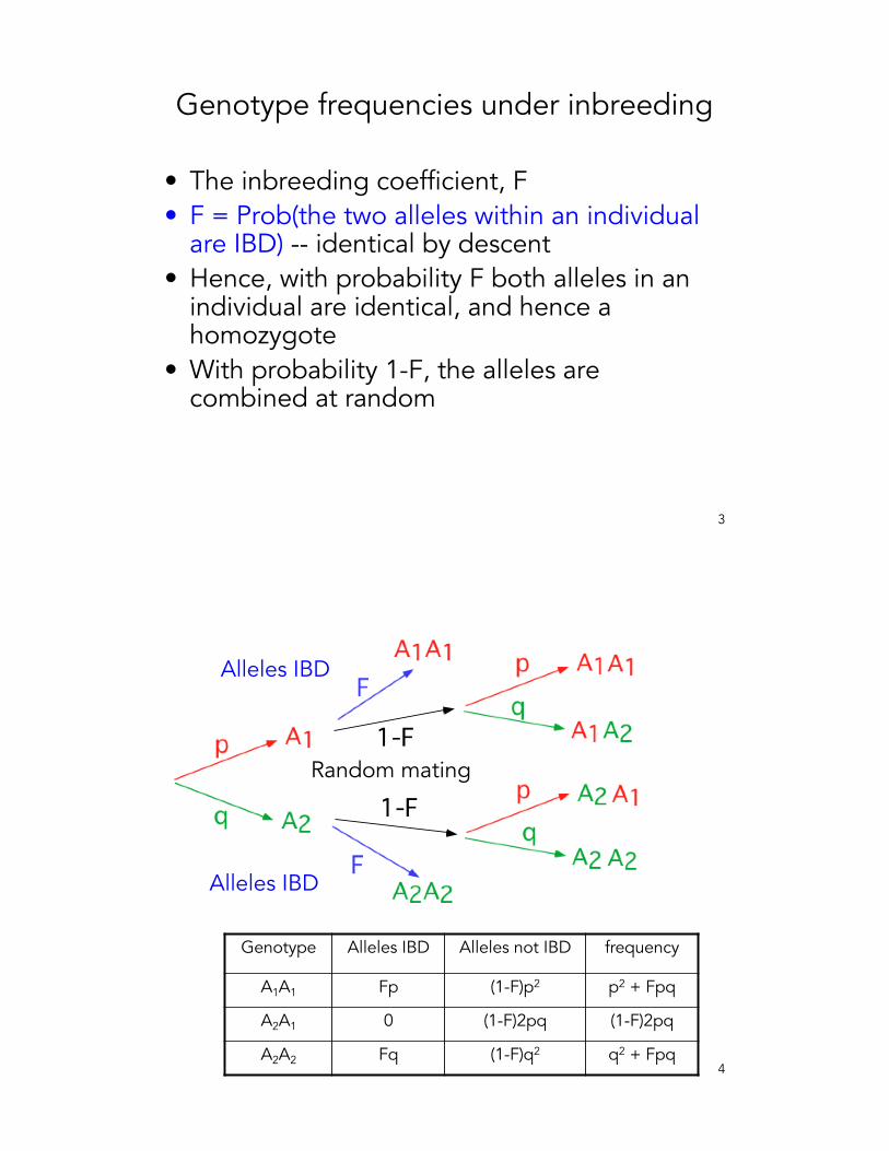
Genotype frequencies under inbreeding

• The inbreeding coefficient, F• F = Prob(the two alleles within an individual

are IBD) -- identical by descent• Hence, with probability F both alleles in an

individual are identical, and hence a homozygote

• With probability 1-F, the alleles are combined at random

4

Genotype Alleles IBD Alleles not IBD frequency

A1A1 Fp (1-F)p2 p2 + Fpq

A2A1 0 (1-F)2pq (1-F)2pq

A2A2 Fq (1-F)q2 q2 + Fpq

Alleles IBD

1-F

1-FRandom mating

Alleles IBD

5

Changes in the mean under inbreeding

µF = µ0 - 2Fpqd

Using the genotypic frequencies under inbreeding, the population mean µF under a level of inbreeding F isrelated to the mean µ0 under random mating by

Genotypes A1A1 A1A2 A2A20 a+d 2a

freq(A1) = p, freq(A2) = q

6

• There will be a change of mean value if dominance is present (d not 0)

• For a single locus, if d > 0, inbreeding will decrease the mean value of the trait. If d < 0, inbreeding will increase the mean

• For multiple loci, a decrease (inbreeding depression) requires directional dominance --- dominance effects di tending to be positive.

• The magnitude of the change of mean on inbreeding depends on gene frequency, and is greatest when p = q = 0.5

7

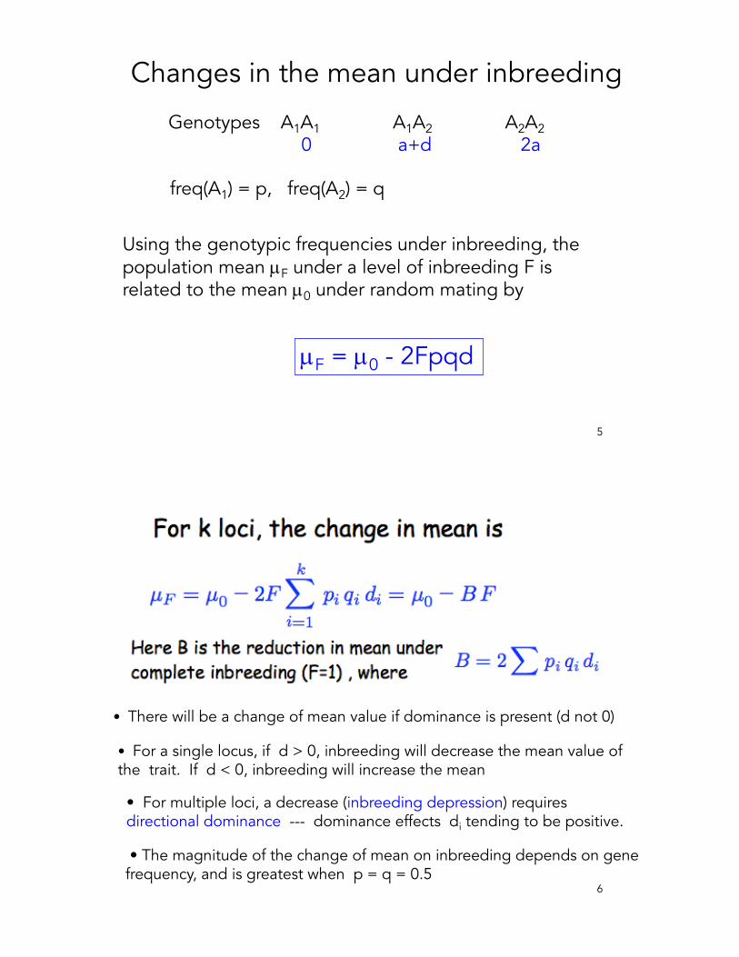
Inbreeding Depression and Fitness traits

Inbred Outbred

8

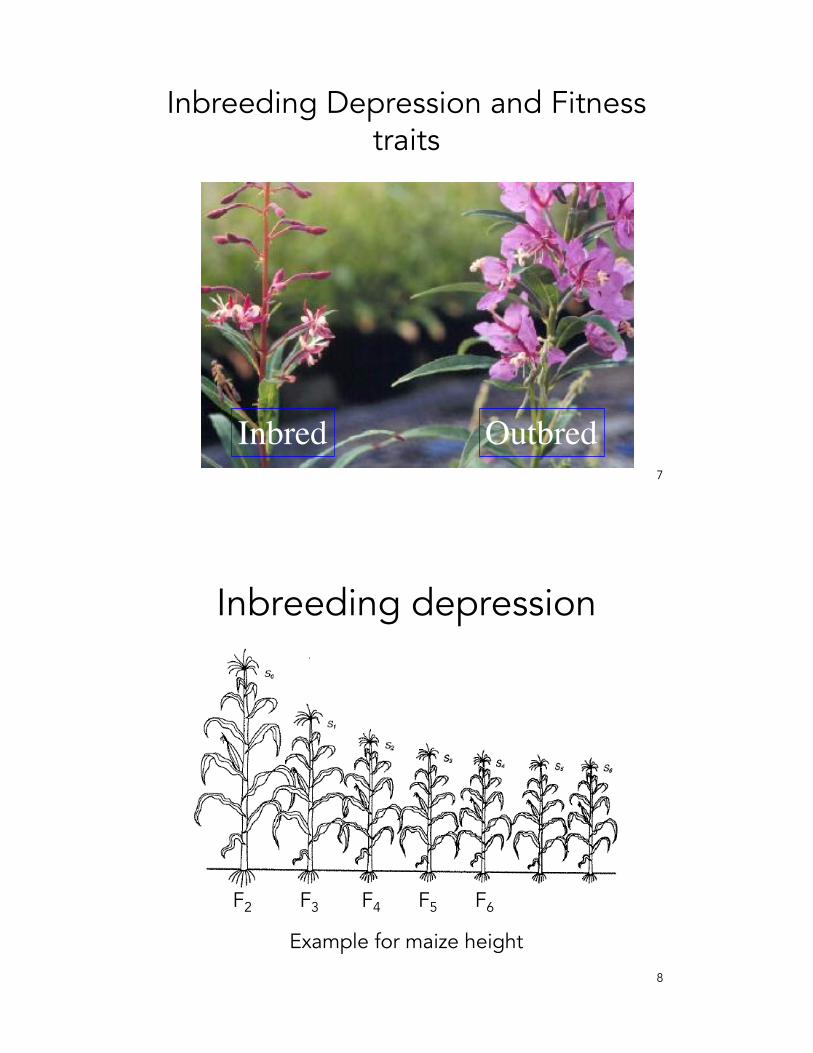
Inbreeding depression

Example for maize height

F2 F3 F4 F5 F6

9

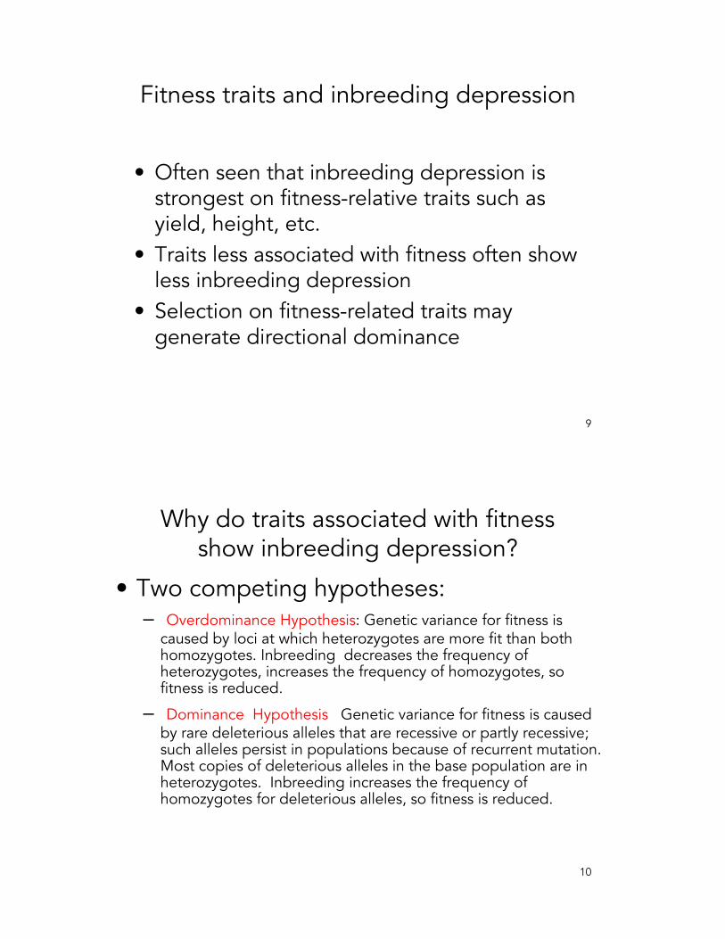
Fitness traits and inbreeding depression

• Often seen that inbreeding depression is strongest on fitness-relative traits such as yield, height, etc.

• Traits less associated with fitness often show less inbreeding depression

• Selection on fitness-related traits may generate directional dominance

10

Why do traits associated with fitness show inbreeding depression?

• Two competing hypotheses:– Overdominance Hypothesis: Genetic variance for fitness is

caused by loci at which heterozygotes are more fit than both homozygotes. Inbreeding decreases the frequency of heterozygotes, increases the frequency of homozygotes, so fitness is reduced.

– Dominance Hypothesis: Genetic variance for fitness is caused by rare deleterious alleles that are recessive or partly recessive; such alleles persist in populations because of recurrent mutation. Most copies of deleterious alleles in the base population are in heterozygotes. Inbreeding increases the frequency of homozygotes for deleterious alleles, so fitness is reduced.

11

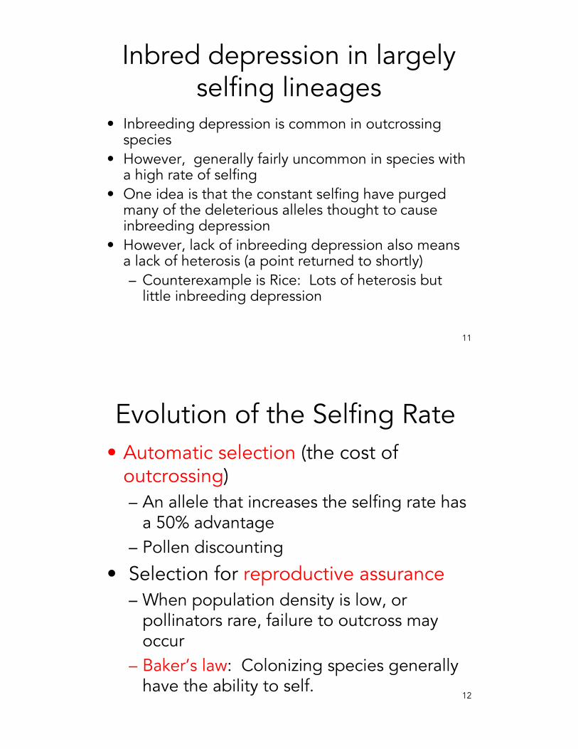
Inbred depression in largely selfing lineages

• Inbreeding depression is common in outcrossing species

• However, generally fairly uncommon in species with a high rate of selfing

• One idea is that the constant selfing have purged many of the deleterious alleles thought to cause inbreeding depression

• However, lack of inbreeding depression also means a lack of heterosis (a point returned to shortly)– Counterexample is Rice: Lots of heterosis but

little inbreeding depression

Evolution of the Selfing Rate• Automatic selection (the cost of

outcrossing)– An allele that increases the selfing rate has

a 50% advantage– Pollen discounting

• Selection for reproductive assurance– When population density is low, or

pollinators rare, failure to outcross may occur

– Baker’s law: Colonizing species generally have the ability to self.

12

13

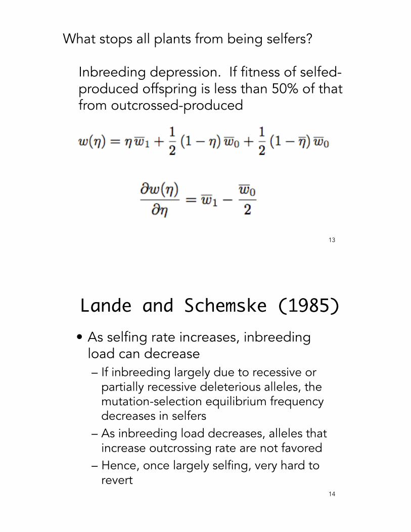
What stops all plants from being selfers?

Inbreeding depression. If fitness of selfed-produced offspring is less than 50% of that from outcrossed-produced

Lande and Schemske (1985)• As selfing rate increases, inbreeding

load can decrease– If inbreeding largely due to recessive or

partially recessive deleterious alleles, the mutation-selection equilibrium frequency decreases in selfers

– As inbreeding load decreases, alleles that increase outcrossing rate are not favored

– Hence, once largely selfing, very hard to revert

14

15

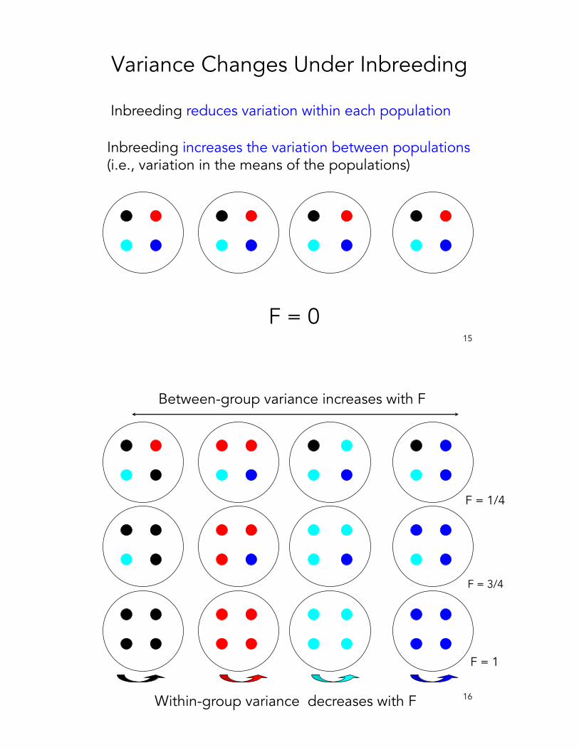
Variance Changes Under Inbreeding

Inbreeding reduces variation within each population

Inbreeding increases the variation between populations(i.e., variation in the means of the populations)

F = 0

16

F = 1/4

F = 3/4

F = 1

Between-group variance increases with F

Within-group variance decreases with F

17

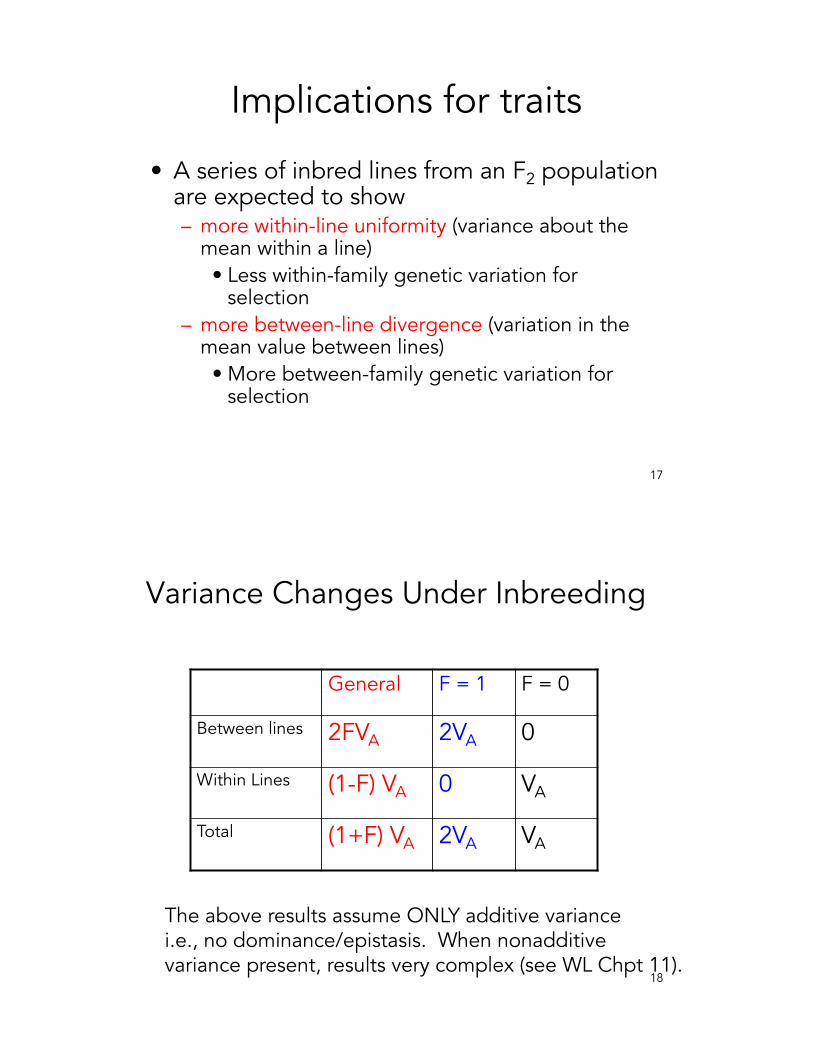
Implications for traits

• A series of inbred lines from an F2 population are expected to show – more within-line uniformity (variance about the

mean within a line) • Less within-family genetic variation for

selection– more between-line divergence (variation in the

mean value between lines)• More between-family genetic variation for

selection

18

Variance Changes Under Inbreeding

General F = 1 F = 0

Between lines 2FVA 2VA 0

Within Lines (1-F) VA 0 VA

Total (1+F) VA 2VA VA

The above results assume ONLY additive variancei.e., no dominance/epistasis. When nonadditivevariance present, results very complex (see WL Chpt 11).

19

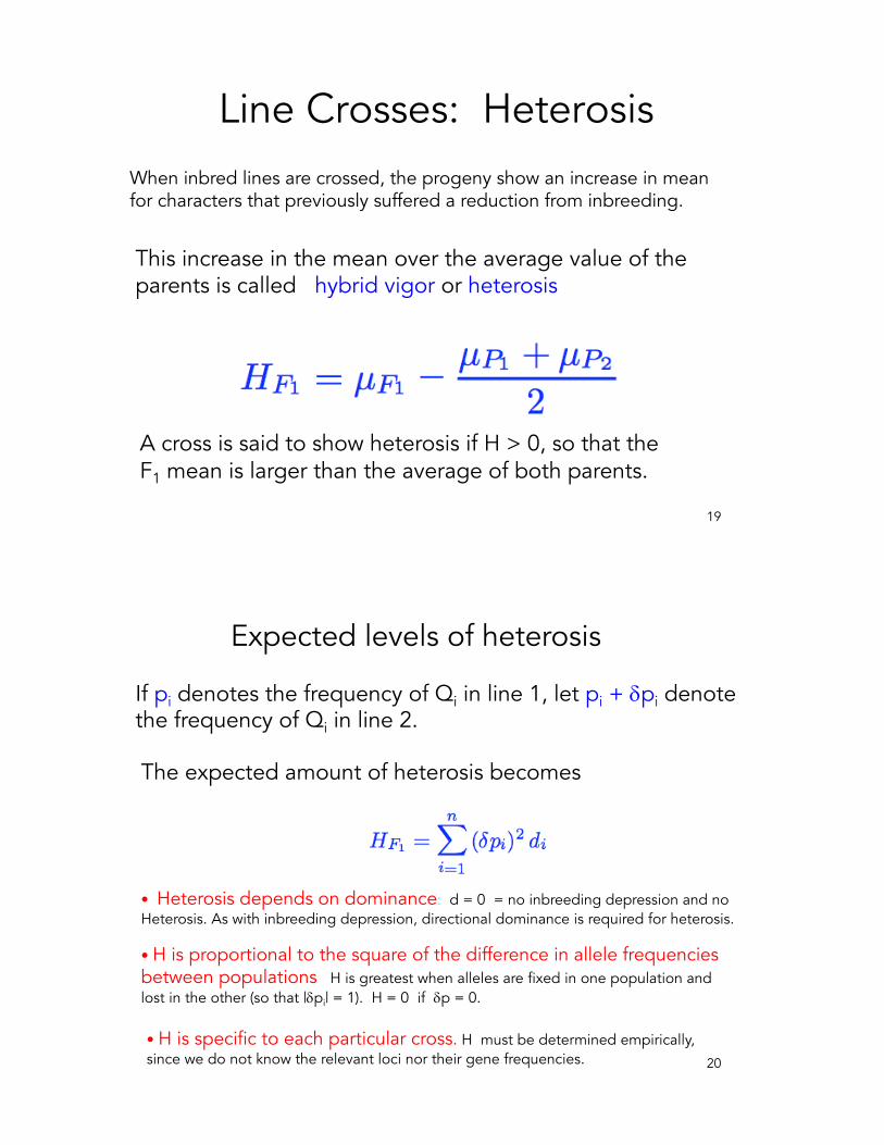
Line Crosses: HeterosisWhen inbred lines are crossed, the progeny show an increase in meanfor characters that previously suffered a reduction from inbreeding.

This increase in the mean over the average value of theparents is called hybrid vigor or heterosis

A cross is said to show heterosis if H > 0, so that the F1 mean is larger than the average of both parents.

20

Expected levels of heterosis

If pi denotes the frequency of Qi in line 1, let pi + dpi denotethe frequency of Qi in line 2.

• Heterosis depends on dominance: d = 0 = no inbreeding depression and no Heterosis. As with inbreeding depression, directional dominance is required for heterosis.

• H is proportional to the square of the difference in allele frequencies between populations. H is greatest when alleles are fixed in one population andlost in the other (so that |dpi| = 1). H = 0 if dp = 0.

• H is specific to each particular cross. H must be determined empirically,since we do not know the relevant loci nor their gene frequencies.

The expected amount of heterosis becomes

HF1 =nX

i= 1

(�pi )2 di

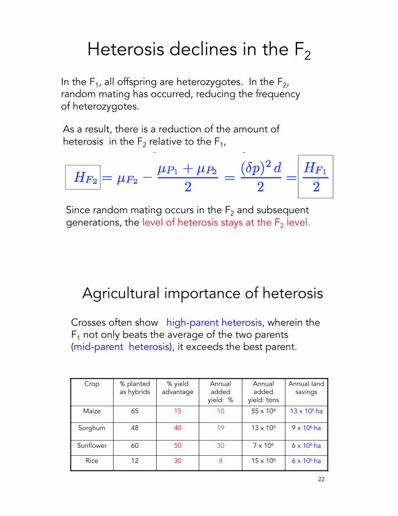
Heterosis declines in the F2

In the F1, all offspring are heterozygotes. In the F2, random mating has occurred, reducing the frequency of heterozygotes.

As a result, there is a reduction of the amount of heterosis in the F2 relative to the F1,

Since random mating occurs in the F2 and subsequentgenerations, the level of heterosis stays at the F2 level.

22

Agricultural importance of heterosis

Crop % planted as hybrids

% yield advantage

Annual added

yield: %

Annual added

yield: tons

Annual land savings

Maize 65 15 10 55 x 106 13 x 106 ha

Sorghum 48 40 19 13 x 106 9 x 106 ha

Sunflower 60 50 30 7 x 106 6 x 106 ha

Rice 12 30 4 15 x 106 6 x 106 ha

Crosses often show high-parent heterosis, wherein the F1 not only beats the average of the two parents (mid-parent heterosis), it exceeds the best parent.

23

Hybrid Corn in the US

Shull (1908) suggested objective of corn breeders should be to find and maintain the best parentallines for crosses

Initial problem: early inbred lines had low seed set

Solution (Jones 1918): use a hybrid line as the seed parent, as it should show heterosis for seed set

1930’s - 1960’s: most corn produced by double crosses

Since 1970’s most from single crosses

24

A Cautionary Tale1970-1971 the great Southern Corn Leaf Blight almost destroyed the whole US corn crop

Much larger (in terms of food energy) than the great potato blight of the 1840’s

Cause: Corn can self-fertilize, so to make hybrids either have to manually detassle the pollen structures or use genetic tricks that cause male sterility.

Almost 85% of US corn in 1970 had Texas cytoplasm Tcms, a mtDNA encoded male sterility gene

Tcms turned out to be hyper-sensitive to the fungusHelminthosporium maydis. Resulted in over a billion dollarsof crop loss

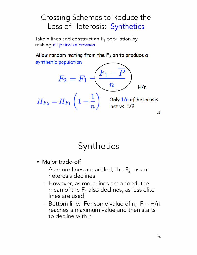
Crossing Schemes to Reduce the Loss of Heterosis: Synthetics

Take n lines and construct an F1 population bymaking all pairwise crosses

26

Synthetics

• Major trade-off– As more lines are added, the F2 loss of

heterosis declines– However, as more lines are added, the

mean of the F1 also declines, as less elite lines are used

– Bottom line: For some value of n, F1 - H/n reaches a maximum value and then starts to decline with n

27

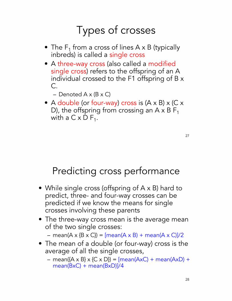
Types of crosses• The F1 from a cross of lines A x B (typically

inbreds) is called a single cross• A three-way cross (also called a modified

single cross) refers to the offspring of an A individual crossed to the F1 offspring of B x C.– Denoted A x (B x C)

• A double (or four-way) cross is (A x B) x (C x D), the offspring from crossing an A x B F1with a C x D F1.

28

Predicting cross performance

• While single cross (offspring of A x B) hard to predict, three- and four-way crosses can be predicted if we know the means for single crosses involving these parents

• The three-way cross mean is the average mean of the two single crosses:– mean(A x {B x C}) = [mean(A x B) + mean(A x C)]/2

• The mean of a double (or four-way) cross is the average of all the single crosses,– mean({A x B} x {C x D}) = [mean(AxC) + mean(AxD) +

mean(BxC) + mean(BxD)]/4

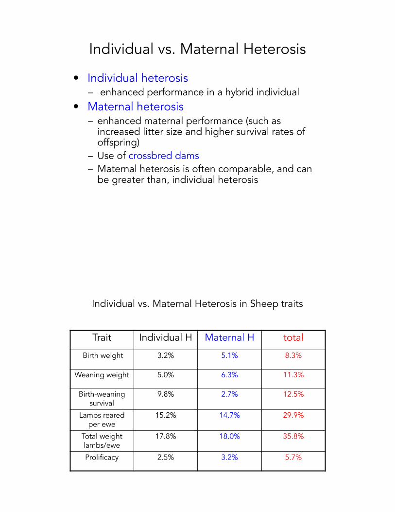
Individual vs. Maternal Heterosis

• Individual heterosis– enhanced performance in a hybrid individual

• Maternal heterosis– enhanced maternal performance (such as

increased litter size and higher survival rates of offspring)

– Use of crossbred dams– Maternal heterosis is often comparable, and can

be greater than, individual heterosis

Individual vs. Maternal Heterosis in Sheep traits

Trait Individual H Maternal H total

Birth weight 3.2% 5.1% 8.3%

Weaning weight 5.0% 6.3% 11.3%

Birth-weaning survival

9.8% 2.7% 12.5%

Lambs reared per ewe

15.2% 14.7% 29.9%

Total weight lambs/ewe

17.8% 18.0% 35.8%

Prolificacy 2.5% 3.2% 5.7%

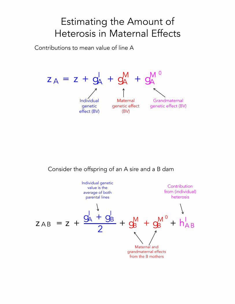
Estimating the Amount of Heterosis in Maternal Effects

z A = z + gIA + gM

A + gM 0

A

Contributions to mean value of line A

Individual genetic

effect (BV)

Maternal genetic effect

(BV)

Grandmaternal genetic effect (BV)

z A B = z +gI

A + gIB

2+ gM

B + gM 0

B + hIA B

Consider the offspring of an A sire and a B dam

Individual genetic value is the

average of both parental lines

Maternal and grandmaternal effects

from the B mothers

Contribution from (individual)

heterosis

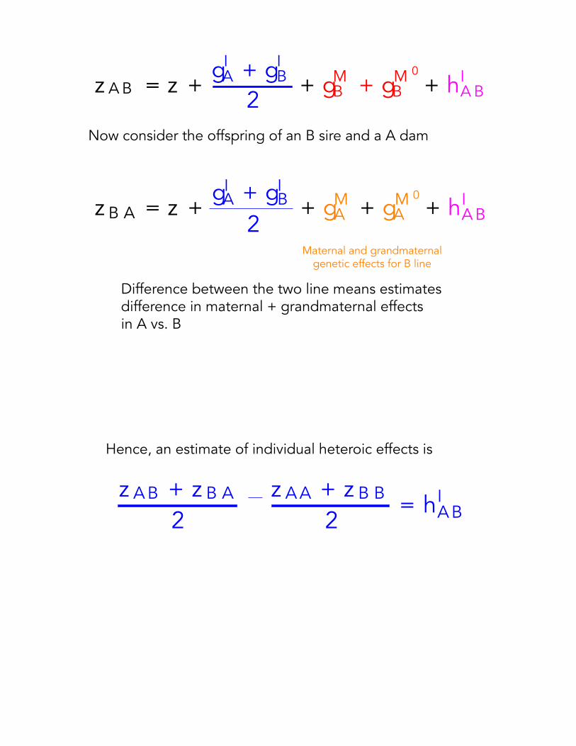
z B A = z +gI

A + gIB

2+ gM

A + gM 0

A + hIA B

Now consider the offspring of an B sire and a A dam

Maternal and grandmaternal genetic effects for B line

z A B = z +gI

A + gIB

2+ gM

B + gM 0

B + hIA B

Difference between the two line means estimatesdifference in maternal + grandmaternal effectsin A vs. B

z A B + z B A

2z A A + z B B

2= hI

A B

Hence, an estimate of individual heteroic effects is

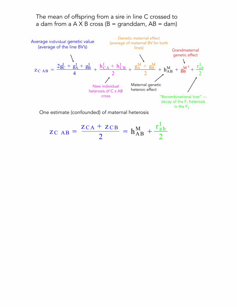
z C AB =2gIC + gIA + gIB

4+hICA + hICB

2+gMA + gMB

2+ hMAB + g

M 0

B +r Ia b2

The mean of offspring from a sire in line C crossed toa dam from a A X B cross (B = granddam, AB = dam)

Average individual genetic value(average of the line BV’s)

New individual heterosis of C x AB

cross

Genetic maternal effect (average of maternal BV for both

lines) Grandmaternal genetic effect

Maternal genetic heteroic effect

“Recombinational loss” ---decay of the F1 heterosis

in the F2

z C AB =z CA + z CB

2= hMAB +

r Ia b2

One estimate (confounded) of maternal heterosis