Lecture 30 - Iowa State Universityclass.ece.iastate.edu/ee435/lectures/EE 435 Lect 30 Spring 2016.pdf · EE 435 Lecture 30 Spectral Performance –Windowing Spectral Performance of

EE 435

Lecture 30

Spectral Performance – Windowing

Spectral Performance of Data Converters- Time Quantization

- Amplitude Quantization

Quantization Noise

Distortion AnalysisT

TS

hm0mNΧN

2A Pm 1

0kΧ

THEOREM?: If NP is an integer and x(t) is band limited to

fMAX, then

and for all k not defined above

where is the DFT of the sequence

f = 1/T, , and

1N

0kkΧ

1N

0kSkTx

MAXP

f Nf = •

2 N

MAXfh = Int

f

.• •

• •

•

R

evie

w f

rom

last

lectu

re .•

•

• •

•

Spectral Response (expressed in dB)

Note Magnitude is Symmetric wrt fSAMPLEP

SIGNALAXISN

1nff

(Actually Stem plots but points connected

in plotting program)

.• •

• •

•

R

evie

w f

rom

last

lectu

re .•

•

• •

•

Spectral Response with Non-coherent Sampling.•

•

• •

•

R

evie

w f

rom

last

lectu

re .•

•

• •

•

(zoomed in around fundamental)

Observations

• Modest change in sampling window of

0.001 out of 20 periods (.0005%) results in

a small error in both fundamental and

harmonic

• More importantly, substantial raise in the

computational noise floor !!! (from over -

300dB to only -80dB)

• Errors at about the 13-bit level !

.• •

• •

•

R

evie

w f

rom

last

lectu

re .•

•

• •

•

Effects of High-Frequency Spectral Components.•

•

• •

•

R

evie

w f

rom

last

lectu

re .•

•

• •

•

Observations

• Aliasing will occur if the band-limited part of the hypothesis for using the DFT is not satisfied

• Modest aliasing will cause high frequency components that may or may not appear at a harmonic frequency

• More egregious aliasing can introduce components near or on top of fundamental and lower-order harmonics

• Important to avoid aliasing if the DFT is used for spectral characterization

.• •

• •

•

R

evie

w f

rom

last

lectu

re .•

•

• •

•

Considerations for Spectral

Characterization

• Tool Validation

• FFT Length

• Importance of Satisfying Hypothesis- NP is an integer

- Band-limited excitation

• Windowing

Are there any strategies to address the

problem of requiring precisely an integral

number of periods to use the FFT?

Windowing is sometimes used

Windowing is sometimes misused

WindowingWindowing is the weighting of the time

domain function to maintain continuity at

the end points of the sample window

Well-studied window functions:

• Rectangular (also with appended zeros)

• Triangular

• Hamming

• Hanning

• Blackman

Rectangular Window

Sometimes termed a boxcar window

Uniform weight

Can append zeros

Without appending zeros equivalent to no window

Rectangular Window

)sin(.)sin( t250tVIN

Assume fSIG=50Hz

Consider NP=20.1 N=512

SIGπf2ω

Rectangular Window


Spectral Response with Non-coherent sampling

Rectangular Window

Columns 1 through 7

-48.8444 -48.7188 -48.3569 -47.7963 -47.0835 -46.2613 -45.3620

Columns 8 through 14

-44.4065 -43.4052 -42.3602 -41.2670 -40.1146 -38.8851 -37.5520


-36.0756 -34.3940 -32.4043 -29.9158 -26.5087 -20.9064 -0.1352


-19.3242 -25.9731 -29.8688 -32.7423 -35.1205 -37.2500 -39.2831


-41.3375 -43.5152 -45.8626 -48.0945 -48.8606 -46.9417 -43.7344

Rectangular Window

Columns 1 through 7

-48.8444 -48.7188 -48.3569 -47.7963 -47.0835 -46.2613 -45.3620


-44.4065 -43.4052 -42.3602 -41.2670 -40.1146 -38.8851 -37.5520


-36.0756 -34.3940 -32.4043 -29.9158 -26.5087 -20.9064 -0.1352


-19.3242 -25.9731 -29.8688 -32.7423 -35.1205 -37.2500 -39.2831


-41.3375 -43.5152 -45.8626 -48.0945 -48.8606 -46.9417 -43.7344

Energy spread over several frequency components

Rectangular Window (with appended zeros)

Triangular Window

Triangular Window


Spectral Response with Non-Coherent Sampling and Windowing

Triangular Window

Triangular Window

Columns 1 through 7

-100.8530 -72.0528 -99.1401 -68.0110 -95.8741 -63.9944 -92.5170


-60.3216 -88.7000 -56.7717 -85.8679 -52.8256 -82.1689 -48.3134


-77.0594 -42.4247 -70.3128 -33.7318 -58.8762 -15.7333 -6.0918


-12.2463 -57.0917 -32.5077 -68.9492 -41.3993 -74.6234 -46.8037


-77.0686 -50.1054 -77.0980 -51.5317 -75.1218 -50.8522 -71.2410

Hamming Window

Hamming Window



Comparison with Rectangular Window

Hamming Window

Columns 1 through 7

-70.8278 -70.6955 -70.3703 -69.8555 -69.1502 -68.3632 -67.5133


-66.5945 -65.6321 -64.6276 -63.6635 -62.6204 -61.5590 -60.4199


-59.3204 -58.3582 -57.8735 -60.2994 -52.6273 -14.4702 -5.4343


-11.2659 -45.2190 -67.9926 -60.1662 -60.1710 -61.2796 -62.7277


-64.3642 -66.2048 -68.2460 -70.1835 -71.1529 -70.2800 -68.1145

Hanning Window

Hanning Window



Comparison with Rectangular Window

Hanning Window

Columns 1 through 7

-107.3123 -106.7939 -105.3421 -101.9488 -98.3043 -96.6522 -93.0343


-92.4519 -90.4372 -87.7977 -84.9554 -81.8956 -79.3520 -75.8944


-72.0479 -67.4602 -61.7543 -54.2042 -42.9597 -13.4511 -6.0601


-10.8267 -40.4480 -53.3906 -61.8561 -68.3601 -73.9966 -79.0757


-84.4318 -92.7280 -99.4046 -89.0799 -83.4211 -78.5955 -73.9788

Comparison of 4 windows


Preliminary Observations about Windows

• Provide separation of spectral components

• Energy can be accumulated around

spectral components

• Simple to apply

• Some windows work much better than

others

But – windows do not provide dramatic

improvement and …

Comparison of 4 windows when sampling

hypothesis are satisfied


Preliminary Observations about Windows

• Provide separation of spectral components

• Energy can be accumulated around

spectral components

• Simple to apply

• Some windows work much better than

others

But – windows do not provide dramatic

improvement and can significantly degrade

performance if sampling hypothesis are met

Issues of Concern for Spectral Analysis

An integral number of periods is critical for spectral analysis

Not easy to satisfy this requirement in the laboratory

Windowing can help but can hurt as well

Out of band energy can be reflected back into bands of interest

Characterization of CAD tool environment is essential

Spectral Characterization of high-resolution data converters

requires particularly critical consideration to avoid simulations or

measurements from masking real performance

• Distortion Analysis

• Time Quantization Effects

– of DACs

– of ADCs

• Amplitude Quantization Effects

– of DACs

– of ADCs

Spectral Characterization of Data

Converters

Will leave the issues of time-quantization and

DAC characterization to the student

These concepts are investigated in the following

slides

Concepts are important but time limitations

preclude spending more time on these topics in

this course

Skip to Next Yellow Slide

Few comments from slides 103-107



– of DACs

– of ADCs


– of DACs

– of ADCs


Converters

Quantization Effects on Spectral

Performance and Noise Floor in DFT

Matlab File: afft_Quantization.m

• Assume the effective clock rate (for either an ADC or a DAC) is arbitrarily

fast

• Without Loss of Generality it will be assumed that fSIG=50Hz

• Index on DFT will be listed in terms of frequency (rather than index number)

Quantization Effects

16,384 pts res = 4bits NP=2520 msec


16,384 pts res = 4bits NP=2520 msec


16,384 pts res = 4bits


Simulation environment:

NP=23

fSIG=50Hz

VREF: -1V, 1V

Res: will be varied

N=2n will be varied

Quantization EffectsRes = 4 bits


Axis of Symmetry


Some components

very small


Set lower display

limit at -120dB








Fundamental














Res 10 No. points 256 fsig= 50.00 No. Periods 23.00

Rectangular Window

Columns 1 through 5

-55.7419 -120.0000 -85.1461 -106.1614 -89.2395


-102.3822 -99.5653 -85.7335 -89.1227 -83.0851



-87.5203 -78.5459 -93.9801 -89.8324 -94.5461


-77.6478 -80.8867 -100.8153 -78.7936 -86.2954


-85.8697 -79.5073 -101.6929 -0.0004 -83.6600


-83.3148 -74.8410 -89.7384 -91.5556 -86.9109


-93.0155 -82.1062 -78.4561 -98.7568 -109.4766


-98.2999 -84.9383 -115.7328 -100.0758 -77.1246


-86.6455 -82.5379 -98.8707 -111.1638 -85.9572


-85.7575 -92.6227 -83.7312 -83.4865 -82.4473


-77.4085 -88.0611 -84.5256 -98.4813 -82.7990


-86.0396 -83.8284 -87.2621 -97.6189 -94.7694


-86.9239 -89.5881 -82.8701 -95.5137 -82.3502


-74.9482 -83.4468 -94.0629 -95.3199 -95.4482


-107.0215 -98.3102 -87.4623 -82.4935 -98.6972


-83.1902 -82.2598 -103.0396 -87.2043 -79.1829


-76.6723 -87.0770 -91.5964 -82.1222 -78.7656


-82.9621 -93.0224 -116.8549 -93.7327 -75.6231


-94.4914 -81.0819

Res 10 No. points 4096 fsig= 50.00 No. Periods 23.00

Rectangular Window

Columns 1 through 5

-55.6060 -97.9951 -107.4593 -103.4508 -120.0000


-96.7808 -105.2905 -96.7395 -104.5281 -90.7582


-85.6641 -101.5338 -120.0000 -87.9656 -99.8947


-108.1949 -90.9072 -111.7312 -120.0000 -117.6276


-97.1804 -102.6126 -111.4008 -0.0003 -97.1838


-97.8440 -101.0469 -102.0869 -93.8246 -101.0151


-104.3215 -100.3451 -97.1556 -86.0534 -94.7263


-96.6002 -91.5631 -105.9608 -116.1846 -91.7843


-96.9903 -91.2626 -102.3499 -97.1841 -99.2579


-91.7837 -102.1146 -98.7668 -98.8830 -120.0000


-108.2877 -110.9318 -97.5933 -94.4604 -99.6057


-91.1056 -101.5798 -94.1031 -95.9163 -83.8407


-93.2650 -103.4274 -103.9702 -98.4092 -91.1825


-98.0638 -93.7989 -107.7453 -93.4277 -88.0409


-107.3584 -102.5984 -95.3312 -102.9342 -108.5206


-99.6667 -97.1966 -94.8552 -92.3877 -84.6006


-96.5194 -85.8129 -95.1970 -94.8699 -104.9224


Res = 10 bitsWith Vin=2v pp

With Vin=1*.99 and Vos=.25LSB

With Vin = 1.999999 pp

With Vin=1*.99 and Vos=.35LSB

Res 10 No. points 4096 fsig= 50.00 No. Periods 25.00 Tstep

1.220703e-004

Magnitude of Fundamental 1.000 2nd Harmonic 0.000

Columns 1 through 7

-56.6785 -65.4098 -66.2097 -65.5916 -66.2436 -66.0461 -66.2097


-66.9055 -66.2436 -66.1762 -66.2097 -65.6639 -66.2436 -65.7315


-66.2097 -66.2800 -66.2436 -66.6393 -66.2097 -65.4202 -66.2436


-66.1363 -66.2097 -65.6765 -66.2436 -0.0044 -66.2097 -65.7635


-66.2436 -66.2196 -66.2097 -66.0852 -66.2436 -66.4771 -66.2097

Res = 10 bits








Quantization Effects16,384 pts res = 4bits


16,384 pts res = 4bits

Res = 10 bits




– of DACs

– of ADCs


– of DACs

– of ADCs


Converters

Spectral Characteristics of

DACs and ADCs

Spectral Characteristics of DAC

t

Periodic Input Signal

Sampling Clock

TSIG t

Sampled Input Signal (showing time points where samples taken)


TSIG

TPERIOD

Quantized Sampled Input Signal (with zero-order sample and hold)

Quantization

Levels


Sampling Clock

TSIG

TPERIOD

TDFT WINDOW

TCLOCK

DFT Clock

TDFT CLOCK


Sampling Clock

TSIG

TPERIOD

TDFT WINDOW

TCLOCK

DFT Clock

TDFT CLOCK


Sampling Clock

DFT Clock


Sampling Clock

DFT Clock

Sampled

Quantized Signal

(zoomed)

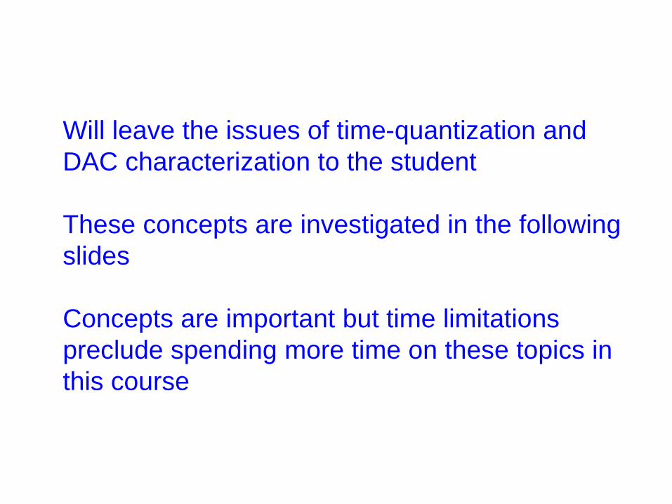
Consider the following example– fSIG=50Hz

– k1=230

– k2=23

– NP=1

– nres=8bits

– Xin(t) =.95sin(2πfSIGt) (-.4455dB)

Thus– NP1=23

– θSR=5

– fCL/fSIG=10

Matlab File: afft_Quantization_DAC.m


nsam = 142.4696

DFT Simulation from Matlab

nsam = 142.4696

DFT Simulation from MatlabExpanded View

Width of this region is fCL

Analogous to the overall DFT window when directly sampled but modestly asymmetric

nsam = 142.4696


nsam = 142.4696


nsam = 142.4696


Columns 1 through 7

-44.0825 -84.2069 -118.6751 -89.2265 -120.0000 -76.0893 -120.0000


-90.3321 -120.0000 -69.9163 -120.0000 -88.9097 -120.0000 -85.1896


-120.0000 -83.0183 -109.4722 -89.4980 -120.0000 -79.6110 -120.0000


-90.2992 -120.0000 -0.5960 -120.0000 -88.5446 -120.0000 -86.0169


-120.0000 -81.5409 -109.6386 -89.7275 -120.0000 -81.8340 -120.0000

fSIG=50Hz , k1=23, k2=23, NP=1, nres=8bits Xin(t) =sin(2πfSIGt)

N=32768


-90.2331 -120.0000 -69.4356 -120.0000 -88.1400 -120.0000 -86.7214


-120.0000 -79.6273 -119.1428 -89.9175 -56.7024 -83.0511 -120.0000


-90.1331 -120.0000 -75.1821 -120.0000 -87.5706 -120.0000 -87.3205


-120.0000 -76.9769 -120.0000 -90.0703 -119.0588 -83.2950 -113.3964


-89.9982 -120.0000 -78.4288 -120.0000 -87.0328 -120.0000 -64.5409

N=32768



-120.0000 -72.8111 -120.0000 -90.1876 -120.0000 -82.5616 -114.0867


-89.8269 -115.6476 -80.6553 -120.0000 -86.3818 -120.0000 -88.3454


-120.0000 -63.5207 -120.0000 -90.2704 -120.0000 -80.8524 -120.0000


-89.6174 -58.5435 -82.3253 -120.0000 -85.6188 -120.0000 -88.7339


-120.0000 -63.8165

N=32768


nsam = 569.8783


nsam = 569.8783


nsam = 569.8783


nsam = 569.8783


Columns 1 through 7

-44.0824 -97.0071 -120.0000 -110.6841 -120.0000 -76.0276 -120.0000


-103.5227 -120.0000 -109.7590 -120.0000 -89.7127 -120.0000 -107.6334


-120.0000 -107.8772 -120.0000 -90.3300 -120.0000 -109.5748 -120.0000


-104.0809 -120.0000 -0.5960 -120.0000 -110.6201 -120.0000 -98.0920


-120.0000 -95.8006 -120.0000 -110.7338 -120.0000 -82.3448 -120.0000


N=131072


-102.9185 -120.0000 -109.9276 -120.0000 -88.8778 -120.0000 -107.5734


-120.0000 -108.1493 -120.0000 -90.7672 -56.7029 -109.3748 -120.0000


-104.5924 -120.0000 -75.3784 -120.0000 -110.5416 -120.0000 -99.0764


-120.0000 -94.4432 -120.0000 -110.7692 -120.0000 -86.1442 -120.0000


-102.2661 -120.0000 -110.0806 -120.0000 -87.7635 -120.0000 -64.4072


N=131072


-120.0000 -108.4202 -120.0000 -91.0476 -120.0000 -109.1589 -120.0000


-105.0508 -120.0000 -81.0390 -120.0000 -110.4486 -120.0000 -99.9756


-120.0000 -92.8919 -120.0000 -110.7904 -120.0000 -88.9028 -120.0000


-101.5617 -58.5437 -110.2183 -120.0000 -86.2629 -120.0000 -105.5980


-120.0000 -108.6808


N=131072


– k1=50

– k2=5

– NP=2

– nres=8bits

– Xin(t) = =.95sin(2πfSIGt) (-.4455dB)

Thus– NP1=5

– θSR=5

– NP2=10


nres=8


nres=8


nres=8


nres=8


Columns 1 through 7

-44.1164 -120.0000 -36.9868 -120.0000 -74.6451 -120.0000 -50.4484


-120.0000 -80.1218 -120.0000 -0.6543 -120.0000 -90.0332 -120.0000


-43.9537 -120.0000 -73.3311 -120.0000 -49.2755 -120.0000 -56.5832


-120.0000 -30.4886 -120.0000 -80.8472 -120.0000 -47.9795 -120.0000


-78.0140 -120.0000 -47.7412 -120.0000 -85.9233 -120.0000 -27.8207

fSIG=50Hz, k1=50, k2=5, NP=2, nres=8bits, Xin(t) =sin(2πfSIGt)

N=131072


-120.0000 -75.9471 -120.0000 -49.8914 -120.0000 -58.4761 -120.0000


-41.7535 -120.0000 -91.4791 -120.0000 -28.1314 -120.0000 -79.7024


-120.0000 -50.5858 -120.0000 -78.7241 -120.0000 -31.9459 -120.0000


-91.9095 -120.0000 -40.4010 -120.0000 -62.1214 -120.0000 -50.1249


-120.0000 -78.2678 -120.0000 -24.9258 -120.0000 -87.6235 -120.0000


N=131072


-45.3926 -120.0000 -77.2183 -120.0000 -48.4567 -120.0000 -76.6666


-120.0000 -30.9406 -120.0000 -69.1777 -120.0000 -48.8912 -120.0000


-75.7581 -120.0000 -44.8212 -120.0000 -88.9694 -120.0000 -19.1255


-120.0000 -79.5390 -120.0000 -50.3103 -120.0000 -70.6123 -120.0000


-38.8332 -120.0000 -92.1633 -120.0000 -34.7560 -120.0000 -77.1229


N=131072

nres=8


nres=8


Columns 1 through 7

-44.0739 -120.0000 -53.8586 -120.0000 -91.9997 -120.0000 -50.3884


-120.0000 -91.3235 -120.0000 -0.6017 -120.0000 -89.9100 -120.0000


-41.0786 -120.0000 -86.6863 -120.0000 -48.5379 -120.0000 -56.7320


-120.0000 -53.4112 -120.0000 -103.7582 -120.0000 -54.1209 -120.0000


-98.4283 -120.0000 -51.2204 -120.0000 -92.1630 -120.0000 -39.9145


N=1024


-120.0000 -86.0994 -120.0000 -46.4571 -120.0000 -58.5568 -120.0000


-45.7332 -120.0000 -88.7034 -120.0000 -52.7530 -120.0000 -102.0744


-120.0000 -54.2124 -120.0000 -101.8321 -120.0000 -52.6742 -120.0000


-89.3186 -120.0000 -45.3675 -120.0000 -62.0430 -120.0000 -46.7029


-120.0000 -85.3723 -120.0000 -40.6886 -120.0000 -92.0718 -120.0000

N=1024



-51.9029 -120.0000 -98.8650 -120.0000 -54.1376 -120.0000 -103.6450


-120.0000 -53.3554 -120.0000 -68.6244 -120.0000 -48.3107 -120.0000


-85.8692 -120.0000 -41.9049 -120.0000 -89.7301 -120.0000 -19.6301


-120.0000 -91.5501 -120.0000 -50.5392 -120.0000 -92.8884 -120.0000


-53.8928 -120.0000 -104.2832 -120.0000 -53.8225 -120.0000 -91.0209

N=1024



– k1=11

– k2=1

– NP=2

– nres=12bits


Thus– NP1=1

– θSR=11

– NP2=2









– k1=230

– k2=23

– NP=1

– nres=12bits


Thus– NP1=23

– θSR=10

– NP2=23









Columns 1 through 7

-68.1646 -94.7298 -120.0000 -90.8893 -120.0000 -75.8402 -120.0000


-97.7128 -120.0000 -69.7549 -120.0000 -90.5257 -120.0000 -95.1113


-120.0000 -94.3119 -120.0000 -91.2004 -120.0000 -79.4167 -120.0000


-97.6931 -120.0000 -0.5886 -120.0000 -90.1044 -120.0000 -95.4585


-120.0000 -93.8547 -120.0000 -91.4631 -120.0000 -81.9608 -120.0000

fSIG=50Hz k1=230 k2=23 NP=1 nres=12bits Xin(t) = =.95sin(2πfSIGt) (-.4455dB) NP1=23 θSR=10

NP2=23

DFT Simulation from MatlabColumns 36 through 42

-97.6535 -120.0000 -69.6068 -120.0000 -89.6188 -120.0000 -95.7721


-120.0000 -93.3545 -120.0000 -91.6806 -80.7859 -83.9353 -120.0000


-97.5940 -120.0000 -75.5346 -120.0000 -89.0602 -120.0000 -96.0458


-120.0000 -92.8067 -120.0000 -91.8555 -120.0000 -85.5462 -120.0000


-97.5144 -120.0000 -78.9551 -120.0000 -88.4176 -120.0000 -88.0509



-120.0000 -92.2056 -120.0000 -91.9896 -120.0000 -86.9037 -120.0000


-97.4143 -120.0000 -81.3430 -120.0000 -87.6762 -120.0000 -96.6112


-120.0000 -91.5441 -120.0000 -92.0844 -120.0000 -88.0732 -120.0000


-97.2936 -82.6264 -83.1604 -120.0000 -86.8155 -120.0000 -96.8068


-120.0000 -90.8133


– k1=230

– k2=23.1

– NP=1

– nres=12bits


Thus– NP1=23.1

– θSR=9.957

– NP2=23.1






– k1=230

– k2=23

– NP=1

– nres=12bits

– Xin(t) =.88sin(2πfSIGt)+0.1sin(2πfSIGt)

– (-1.11db fundamental, -20dB 2nd harmonic)

Thus– NP1=23

– θSR=10

– NP2=23





Columns 1 through 7

-68.2448 -95.4048 -103.0624 -91.5534 -94.3099 -76.5052 -107.8586


-98.3634 -107.7150 -70.4198 -97.2597 -91.1898 -103.5449 -95.7898


-108.9130 -94.9846 -102.5323 -91.8645 -90.3773 -80.0818 -107.9922


-98.3435 -107.5614 -1.2534 -99.6919 -90.7685 -103.9860 -96.1429


-108.9011 -94.5258 -101.9463 -92.1271 -83.9805 -82.6260 -108.1158

fSIG=50Hz k1=230 k2=23 NP=1 nres=12bits Xin(t) =.88sin(2πfSIGt)+0.1sin(2πfSIGt) (-1.11db

fundamental, -20dB 2nd harmonic) NP1=23 θSR=10 NP2=23



-98.3035 -107.3983 -70.2715 -101.8108 -90.2829 -104.3909 -96.4685


-108.8814 -94.0244 -101.2937 -92.3447 -20.5694 -84.6007 -108.2298


-98.2433 -107.2276 -76.1993 -103.7144 -89.7244 -104.7634 -96.7781


-108.8537 -93.4756 -100.5602 -92.5195 -83.3389 -86.2119 -108.3343


-98.1627 -107.0564 -79.6196 -105.4341 -89.0818 -105.1065 -82.5417



-108.8180 -92.8737 -99.7264 -92.6536 -89.0679 -87.5695 -108.4295


-98.0612 -106.9226 -82.0074 -106.9364 -88.3404 -105.4217 -97.1991


-108.7742 -92.2117 -98.7644 -92.7484 -92.3212 -88.7393 -108.5158


-97.9383 -82.1713 -83.8248 -108.1091 -87.4797 -105.7091 -97.4305


-108.7221 -91.4804 -97.6333 -92.8049 -94.5701 -89.7636 -108.5932

Skip from Previous

Yellow Slide

Summary of time and amplitude

quantization assessment

Time and amplitude quantization do not

introduce harmonic distortion

Time and amplitude quantization do

increase the noise floor

End of Lecture 30

Documents

Lecture 30 - Iowa State Universityclass.ece.iastate.edu/ee435/lectures/EE 435 Lect 30 Spring 2016.pdf · EE 435 Lecture 30 Spectral Performance –Windowing Spectral Performance of