Lecture 3 Efficiency wages - coin.wne.uw.edu.plcoin.wne.uw.edu.pl/wincenciak/docs/makro_zaawansowana/lecture_3.pdf · Lecture3–Efficiencywages Basicmodelofefficiencywages 5/43 Possiblereasonsforefficiencywages

Lecture 3Efficiency wages

Leszek Wincenciak, Ph.D.

University of Warsaw

Lecture 3 – Efficiency wages

2/43

Lecture outline:

Basic model of efficiency wagesPossible reasons for efficiency wagesSimple modelModel interpretationModel implications

More general version of the efficiency-wages modelModel set-upExampleModel implications

Simple model of shirking

Gift exchange – fair wage hypothesis

Efficiency wages as a turnover reduction toolRetainment


Basic model of efficiency wages 3/43

Basic model of efficiency wages



Possible reasons for efficiency wages

Why may firms choose to pay higher than market-clearing wages?

� Nutrition – workers with higher wages may consume morefood thus their health conditions improve and they are moreproductive (developing economies)

� Inability to monitor workers effort – high wage makes losinga job a real punishment for low effort (Shapiro-Stiglitz)

� Higher wages attract high skilled workers (with possibly higherreservation wages) and this increases average skill level of theworkforce hired by the firm

� High wages build loyalty among workers (gift exchange)reducing turnover – high turnover may be costly due tosubstantial costs of hiring and firing. Higher wages my lowerlikelihood that workers will unionize (insiders-outsiders)



Possible reasons for efficiency wages

A historical example

� Raff and Summers (1987) conduct a case study on Henry Ford’sintroduction of the five dollar day in 1914.

� Ford experience supports efficiency wage interpretations. Ford’sdecision to increase wages so dramatically (doubling for mostworkers) is most plausibly portrayed as the consequence of efficiencywage considerations, with the structure being consistent, evidenceof substantial queues for Ford jobs, and significant increases inproductivity and profits at Ford.

� High turnover and poor worker morale appear to have playeda significant role in the five-dollar decision.

� Ford’s new wage put him in the position of rationing jobs, andincreased wages did yield productivity benefits and profits.

� There is also evidence that other firms emulated Ford’s policy tosome extent, with wages in the automobile industry 40% higherthan in the rest of manufacturing (Rae 1965, quoted in Raff andSummers).



Simple model

Basic model of efficiency wages

Assume there is a large number, N , of competitive firms. Therepresentative firm aims at profit maximization:

π = Y − wL, (1)

where Y is the firm’s output, w – the wage it pays and L is theamount of labour it hires. For simplicity, we neglect prices andexpress wages and output in real terms.

Firm’s output is not only a function of the number of workers, butalso of their effort. Assume there are no other inputs:

Y = F (eL), F ′(·) > 0 F ′′(·) < 0. (2)



Simple model

Crucial assumption of efficiency wages model is that the effortdepends positively on wage. Consider first simple case (Solow,1979) where the wage is the only determinant of the effort:

e = e(w), e′(·) > 0. (3)

Finally, we assume that there are L identical workers. Every workersupplies 1 unit of labour inelastically.

The problem of the firm may be rewritten as:

maxL,w

F (e(w)L) − wL. (4)



Simple model

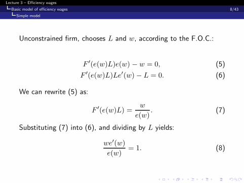
Unconstrained firm, chooses L and w, according to the F.O.C.:

F ′(e(w)L)e(w) − w = 0, (5)

F ′(e(w)L)Le′(w)− L = 0. (6)

We can rewrite (5) as:

F ′(e(w)L) =w

e(w). (7)

Substituting (7) into (6), and dividing by L yields:

we′(w)e(w)

= 1. (8)



Model interpretation

Interpretation – single firm perspective

we′(w)e(w)

= 1. (8)

Equation (8) states that at the optimum, the elasticity of effortwith respect to wage is 1. Remember that firm’s output isa function of effective labour (eL), and that’s why firm wants tohire effective labour as cheaply as possible. When a firm hiresa worker it obtains e(w) units of effective labour at a cost of w.The cost per unit of effective labour is then w/e(w). When theelasticity of e w.r.t. w is 1, a marginal change in w does notchange this ratio, thus this is the first-order condition for theproblem of choosing w to minimize the cost of effective labour.The wage that satisfies (8) is known as the efficiency wage.




Interpretation – single firm perspective

F ′(e(w)L) =w

e(w). (7)

Equation (7) states that the firm hires workers until the marginalproduct of effective labour equals its cost. This is analogous to thecondition in a standard labour demand problem (VMPL = w).




Interpretation – economy-wide perspective

Let w∗ and L∗ denote values of w and L that satisfy (7) and (8).Since all firms are identical, they choose the same values of w andL. Total labour demand is therefore NL∗. If labour supply, L,exceeds this amount, firms are unconstrained in their choice of w.In this case the wage is w∗, employment is NL∗ andunemployment equals L−NL∗. If NL∗ > L then firms areconstrained, wages are bid up to the point where demand andsupply are in balance and there is no unemployment.




e(w)

�

e(w)w

ww∗

e

Figure 1. The determination of the efficiency wage



Model implications

Implications of the basic efficiency-wages model

� Efficiency wages may give rise to unemployment� Real wage does not respond to demand shifts, which influenceemployment only

� Costs of a unit of effective labour are constant, which impliesprice rigidity in price-setting firms

� In the long run, economic growth leading to an outward shiftof labour demand will eventually lead to a decrease inunemployment to zero (because of real wage rigidity). Furtherincrease in labour demand will push real wage up.

� In practice, we do not observe a downward trend ofunemployment in the long run!


More general version of the efficiency-wages model 14/43

More general version of the efficiency-wages model



Model set-up

More general version of the efficiency-wages model

The wage may not be the only determinant of effort. If the firmchooses to pay higher wages to encourage workers to work harderbut cannot monitor their effort perfectly, losing a job is the onlypunishment, when workers were caught shirking. The cost fora worker of being fired depends not only on the lost wage, but alsoon how easy is to find a new job, and what is the alternative wage.Therefore workers (not perfectly observable) effort should behigher, when the unemployment is high, and when the bestpossible alternative wage is low.

e = e(w,wa, u),∂e

∂w> 0,

∂e

∂wa< 0,

∂e

∂u> 0. (9)



Model set-up

Empirical example

Agell & Lundborg (Survey Evidence on Wage Rigidity andUnemployment: Sweden in the 1990s, Scandinavian Journal ofEconomics, 1995) – Survey of 159 Swedish manufacturing firms.

The question:„How do you think the work effort of your employees would beaffected if local unemployment were to rise?”

Increase: 86%.



Model set-up

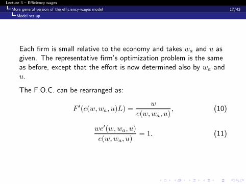
Each firm is small relative to the economy and takes wa and u asgiven. The representative firm’s optimization problem is the sameas before, except that the effort is now determined also by wa andu.

The F.O.C. can be rearranged as:

F ′(e(w,wa, u)L) =w

e(w,wa, u), (10)

we′(w,wa, u)

e(w,wa, u)= 1. (11)



Model set-up

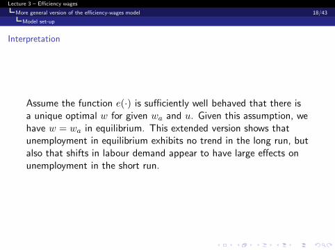
Interpretation

Assume the function e(·) is sufficiently well behaved that there isa unique optimal w for given wa and u. Given this assumption, wehave w = wa in equilibrium. This extended version shows thatunemployment in equilibrium exhibits no trend in the long run, butalso that shifts in labour demand appear to have large effects onunemployment in the short run.



Example

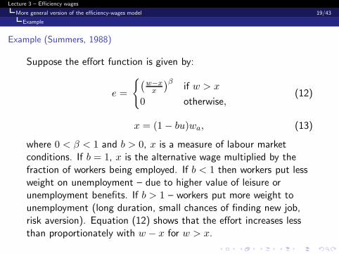
Example (Summers, 1988)

Suppose the effort function is given by:

e =

{(w−xx

)β if w > x

0 otherwise,(12)

x = (1− bu)wa, (13)

where 0 < β < 1 and b > 0, x is a measure of labour marketconditions. If b = 1, x is the alternative wage multiplied by thefraction of workers being employed. If b < 1 then workers put lessweight on unemployment – due to higher value of leisure orunemployment benefits. If b > 1 – workers put more weight tounemployment (long duration, small chances of finding new job,risk aversion). Equation (12) shows that the effort increases lessthan proportionately with w − x for w > x.



Example

Differentiating (12) leads to the condition that elasticity of effortw.r.t. wage is equal 1:

βw

[(w − x)/x]β

(w − x

x

)β−1 1

x= 1. (14)

We can simplify this condition to get:

w =x

1− β=

1− bu

1− βwa (15)

For small values of β, 1/(1 − β) ≈ 1 + β. Therefore (15) impliesthat when β is small, firms offer a premium equal approximatelythe fraction β of the labour market conditions index, x.



Example

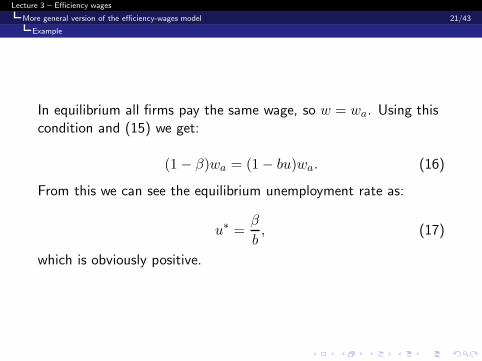
In equilibrium all firms pay the same wage, so w = wa. Using thiscondition and (15) we get:

(1− β)wa = (1− bu)wa. (16)

From this we can see the equilibrium unemployment rate as:

u∗ =β

b, (17)

which is obviously positive.



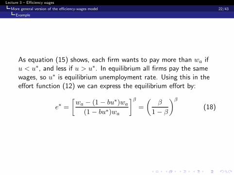
Example

As equation (15) shows, each firm wants to pay more than wa ifu < u∗, and less if u > u∗. In equilibrium all firms pay the samewages, so u∗ is equilibrium unemployment rate. Using this in theeffort function (12) we can express the equilibrium effort by:

e∗ =[wa − (1− bu∗)wa

(1− bu∗)wa

]β=

(β

1− β

)β

(18)



Example

Finally, the equilibrium wage satisfies the condition thatF ′(eL) = w/e equivalent to w = eF ′(eL). Total employment inequilibrium is (1− u∗)L, therefore each firm hires (1− u∗)L/Nworkers. Equilibrium wage is therefore:

w∗ = e∗F ′(e∗(1− u∗)L

N

). (19)



Model implications

Model implications

� Equilibrium unemployment depends only on parameters of theeffort function (see eq. 17), not the production function →upward trend of production is not followed by a trend inunemployment.

� Relatively small values of β – the elasticity of effort w.r.t. thepremium that firms pay over the labour market conditionsindex, x – may lead to nonnegligible unemployment. Forβ = 0.06 and b = 1 or β = 0.03 and b = 0.5 theunemployment rate is 6%.

� With β = 0.03 and b = 0.5, we get u = 6%, but we can alsosee from (13) that the workers exert no effort at all, unlessthe firm pays at least 97% of the alternative wage. Soefficiency-wage forces are very strong for these parametervalues.



Model implications

Model implications

� Using this outcome we can explain why younger people mighthave on average higher unemployment rates. They probablyhave higher value of leisure, which means a lower b. On theother hand they might also have higher elasticity of effortw.r.t. the premium that that firm pays over the labour marketconditions index x. All this together according to (17) leadsto higher unemployment rates


Simple model of shirking 26/43





Assumptions:

Providing effort e causes for a worker a cost φ(e). This cost can beeither real expenditure or loss of welfare (disutility – who likes towork hard???) that must be compensated by higher consumption,if the level of welfare is kept at the same level.

When a firm hires a worker, there is an agreement on the(minimum) efficiency e and the wage w for the worker. The workeris said to shirk, if (s)he works less efficiently than what was agreedon, e < e.




In case of shirking, the worker is either caught and fired, or notcaught and kept in the workplace despite of the too lowproductivity. To simplify the analysis, let’s take two assumptions asfollows: the probability that one is caught for shirking in the firm isa constant θ ∈ (0, 1), and the elasticity of the workers efficiencycost is a constant 1/ε:

φ(e) = μe1/ε,dφ

de

e

φ=

1

ε, μ > 0, ε ∈ (0, 1). (20)

Because φ′′ > 0, the workers effort to improve its efficiency isincreasingly difficult.




Now we see the following:

� The workers income without shirking is equal to the wage inthe firm, w, minus efficiency cost φ(e): w − φ(e)

� The workers income with shirking is equal to the wage in thefirm, w, times the probability of not being caught for shirking,(1− θ), plus the expected wage outside the firm, v, times theprobability of being caught for shirking, θ: (1− θ)w + θv




The worker shirks definitely, if income for that is greater than fornonshirking, (1− θ)w + θv > w − φ(e). Hence, if the employerwants to ensure that the worker does not shirk, there must beincentive comparability constraint imposed:

(1− θ)w + θv � w − φ(e),

which is equivalent to:

w � v +φ(e)

θ. (21)

The firm will choose the lowest possible wage that satisfies thiscondition, so w = v + φ(e)/θ.




We can observe some interesting facts. The wage providingappropriate incentive not to shirk is higher if:

� wages paid outside the firm grow (v ↑)� cost of effort is increasing (φ ↑)� the probability of being caught is low (θ ↓)




From the condition (21) we can state that: φ(e) = θ(w− v). If weuse the definition of the cost function from (20) we get:

e =

(θ

μ

)ε

(w − v)ε

Now if we take the efficiency wages condition that the elasticity ofeffort with respect to wages is equal 1, we get:

ε(

θμ

)ε(w − v)ε−1w(

θμ

)ε(w − v)ε

= 1




After some simplifications we get finally:

w =v

1− ε.

If we adopt that v = (1− u)w + ub, and assume that benefits arepaid as a constant proportion of average wage, so that b = βw, wecan calculate unemployment:

u∗ =ε

1− β

with the same conclusions as before.


Gift exchange – fair wage hypothesis 34/43





Workers have some idea of a ’fair wage’. The fundamental concepthere is the reference group theory. It says that our morale andwillingness to perform depends importantly on what we get relativeto what we see our likes getting. (Akerlof 1982, Akerlof, Yellen1990).The employer chooses w to motivate workers to exert effort e,which will be chosen to maximize workers utility.The workers effort depends on the relation between the fair wage(w) and the actual wage (w) paid by the firm. The fair wage ishigher the higher are expected wages paid by other firms (wa), butit is lower if unemployment is high.



Empirical examples

Armin Falk (Gift Exchange in the Field, IZA Working paper, 2005):

This study reports evidence from a field experiment that wasconducted to investigate the relevance of gift-exchange in a naturalsetting. In collaboration with a charitable organization we sentroughly 10,000 solicitation letters to potential donors. One third ofthe letters contained no gift, one third contained a small gift andone third contained a large gift. The treatment assignment wasrandom. The results confirm the economic importance ofgift-exchange. Compared to the no gift condition, the relativefrequency of donations increased by 17 percent if a small gift wasincluded and by 75 percent for a large gift.



Empirical examples

Fehr and Gachter (2000), Fairness and Retaliation: The Economicsof Reciprocity, Journal of Economic Perspectives, Vol. 14, 159-181.

Reciprocity as a contract enforcement device. The requirement ofa generally cooperative job attitude renders reciprocal motivationspotentially very important in the labor process. If a substantialfraction of the work force is motivated by reciprocityconsiderations, employers can affect the degree of”cooperativeness” of workers by varying the generosity of thecompensation package – even without offering explicit performanceincentives.



Empirical examples

Bellemare and Shearer (2007), Gift Exchange within a Firm:Evidence from a Field Experiment, IZA Discussion Paper no. 2696.

A field experiment testing the gift-exchange hypothesis insidea treeplanting firm paying its workforce incentive contracts. Firmmanagers told a crew of tree planters they would receive a payraise for one day as a result of a surplus not attributable to pastplanting productivity. They compare planter productivity – thenumber of trees planted per day on the day the gift was handedout with productivity on previous and subsequent days of plantingon the same block, and thus under similar planting conditions. Wefind direct evidence that the gift had a significant and positiveeffect on daily planter productivity, controlling for planter-fixedeffects, weather conditions and other random daily shocks.Moreover, reciprocity is the strongest when the relationshipbetween planters and the firm is longterm.



Therefore we can adopt the same notation for workers effort asbefore:

e = e(w+, w−) where w = h(wa

+, u−),

or we can simply write:

e = e

(w

wa, u

)+ +

. (22)

This leads to the same conclusion, that in the optimum the wagewill be chosen in such a way, to make the elasticity of workerseffort w.r.t. wage equal 1.


Efficiency wages as a turnover reduction tool 40/43

Efficiency wages as a turnover reduction tool



Retainment

Retainment

So far we have studied motivating effects of higher wages. Nowlet’s turn to the problems concerning labour turnover. Firms maywish to retain its workers, or at least minimize turnover, becausetraining and hiring new workers induces real costs for the firm.Paying higher wages is a tool to achieve this. Assume, that theworkers quit rate is given by:

q = q(w,wa, u) (qw < 0, qwa > 0, qu < 0). (23)

Whenever a quitter is replaced, the firm must incur training cost θ.The firms steady-state profits are:

π = F (L)− [w + θq(w,wa, u)]L, (24)



Retainment

Clearly, this expression is similar to the one used earlier (see eq. 4).It can be solved by first minimizing the cost per worker (the termin brackets) and then by choosing employment. The equilibriumunemployment is determined by setting w = wa and using quitrate function. It turns out that the equilibrium unemploymentincreases with relative training costs (θ/w) or when exogenousturnover propensities rise.



Retainment

Henry Ford example

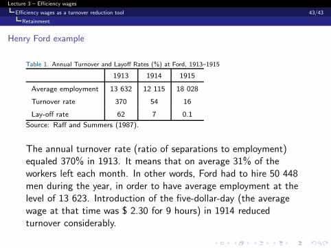
Table 1. Annual Turnover and Layoff Rates (%) at Ford, 1913–1915

1913 1914 1915

Average employment 13 632 12 115 18 028

Turnover rate 370 54 16

Lay-off rate 62 7 0.1

Source: Raff and Summers (1987).

The annual turnover rate (ratio of separations to employment)equaled 370% in 1913. It means that on average 31% of theworkers left each month. In other words, Ford had to hire 50 448men during the year, in order to have average employment at thelevel of 13 623. Introduction of the five-dollar-day (the averagewage at that time was $ 2.30 for 9 hours) in 1914 reducedturnover considerably.

Documents

Lecture 3 Efficiency wages - coin.wne.uw.edu.plcoin.wne.uw.edu.pl/wincenciak/docs/makro_zaawansowana/lecture_3.pdf · Lecture3–Efficiencywages Basicmodelofefficiencywages 5/43 Possiblereasonsforefficiencywages