Embed Size (px)
Citation preview

Lecture 3: Basics of code acquisition
and tracking
TLT-5606
Lecturer: Simona Lohan
Spring 2009
Acknowledgments: These slides are mainly based on the original lecture
notes by prof. Tapani Ristaniemi and Toni Huovinen.

Outline
■ Preliminaries
■ Code acquisition:
● Optimum solution:MAP and ML estimates● Detection probability, false alarms and miss-detections● Code acquisition strategies● Mean acquisition times
■ Code tracking
● Classical Delay Locked Loops (DLL)● S curves
■ Conclusions

Preliminaries
■ In SS techniques the timing information is necessary for
successful despreading and demodulation
■ Timing estimation can be using a two-step approach:
⋆ coarse estimation (initial code acquisition)⋆ fine estimation (code tracking)
■ Acquisition is used to get a rough timing estimate, say within a
duration of a chip, that is, timing uncertainty is ±Tc
■ Tracking means finding and maintaining fine synchronization
■ Code tracking is much easier given the initial acquisition
(delay lock loop)
■ Code acquisition, however, is usually considered as one of
the most challenging tasks in a SS systems

Example 1: despreading with incorrect phase
0 5 10 15
−1
0
1
0 5 10 15
−1
0
1
0 5 10 15
−1
0
1
0 5 10 15
−1
0
1
0 5 10 15
−1
0
1
0 5 10 15
−1
0
1
■ Three left-most figures: narrowband data (uppermost), spreading code ”1
1 -1 -1 1” (middle) and spread data (lowermost). Here, Tc = 1, N = 5,T = NTc = 5.
■ Three right-most figures: despread data with incorrect phase ”1 -1 -1 1 1”
(uppermost), despread data with another incorrect phase ”-1 1 1 1
-1”(middle) and despread data with correct phase (lowermost).

Example 2: previous + multiuser data
0 5 10 15−2
−1
0
1
2
0 5 10 15−2
−1
0
1
2
0 5 10 15−2
−1
0
1
2
0 5 10 15−2
−1
0
1
2
0 5 10 15−2
−1
0
1
2
0 5 10 15−5
0
5
10
■ Three left-most figures: user 1 SS signal s1 (uppermost), user 2 SS signal s2(middle) and received SS signal s1 + 2s2.
■ Three right-most figures: despread user 1 data with incorrect phase
(uppermost), despread user1 data with correct phase (middle) and
”integrate-and-dump” outputs.
■ With incorrect phase (”o”) estimated symbols for user 1 are (sign of the
output at times 5,10,15) ”-1 1 1” while with correct phase (”x”) ”1 -1 1”

Uncertainty regions
■ Timing uncertainty: determined by the transmission time of
the transmitter and the propagation delay
⋆ usually much longer than a chip duration.⋆ due to a search through all possible delays, a larger timinguncertainty means a larger search area
■ Frequency uncertainty: determined by the Doppler shift and
mismatch between the transmitter and receiver oscillators.
■ Angular uncertainty: determined by the direction of arrival of
the signal. Separation in angular domain applies only for
antenna array receivers.
■ Moreover, initial code acquisition must be accomplished in
low SNR environments and in the presence of interferers. The
possibility of channel fading and Multi-User Interference (MUI)
can make initial acquisition even harder to accomplish.

Code acquisition: optimum solution
■ To start with, consider a received signal r(t) = s(t, Θ) + n(t),where Θ contains the parameters (frequency, phase, delay,data,...) to be estimated under Gaussian noise n(t).
■ The best that can be done is to search for an estimate Θ̂ ofthe parameter Θ that maximizes a posteriori probabilityp(Θ|r(t)).
■ In other words, such an estimate Θ̂ is correct for the highestprobability given the observation r(t).
■ This estimate Θ̂ is called the maximum a posteriori (MAP)estimate.
■ In practice, we have to generate a set of candidate values
Θ̃, evaluate p(Θ̃|r) for each candidate and then chooseΘ̂ = Θ̃ for which p(Θ̃|r) is maximum.

■ Next we consider only the temporal parameter estimation,
denoted by θ̃ (i.e., the phase of the spreading code). Then,MAP can be analytically expressed as,
θ̂ = arg max p(θ̃|r) (1)
■ Usually, p(θ̃|r) can not be expressed in closed form. However,by using Bayesian rule for joint probability distribution
functions we have
p(r, θ̃) = p(r)p(θ̃|r) = p(θ̃)p(r|θ̃) (2)
■ Assuming uniform prior distribution for θ̃, then maximization ofp(θ̃|r) becomes equivalent to maximization of p(r|θ̃). This iscalled a maximum likelihood (ML) estimate which analytically
writes
θ̂ = arg max p(r|θ̃) (3)

■ Assuming Gaussian noise, maximizing p(r|θ̃) becomesequivalent to maximizing the likelihood function defined as
λ(θ̃) =
Z
r(t)s(t, θ̃)dt (4)
where s(t, θ̃) is a local copy of the signal when using trialvalue for parameter θ̃.
■ That is,
θ̂ = arg max λ(θ̃) (5)
■ Considering s(t, θ) a DS-CDMA signal, the basic principle forcode acquisition is: try and match each possible phase of the
reference spreading sequence to the received data.

■ In practice, the acquisition process follows a basic working
principle: (BPF=Band Pass Filter, ED= Energy Detector)
Despreading
Referencewaveform
frequency estimate
timing estimateReferencespreadingwaveformgenerator
Decision Received
SS signal
Control
logic
mixer
EDX BPF
⋆ The receiver makes a hypothesis on a phase of thespreading sequence and despreads the received signal
using the hypothesized phase.
⋆ If the hypothesized phase matches to the sequence in thereceived signal, the wide-band SS signal will be despread
correctly into a narrowband information bearing signal

⋆ A bandpass filter (bandwidth similar to that of thenarrowband data) is employed to collect the power of the
despread signal.
⋆ If the hypothesized phase is correct, the BPF will collect allthe power of the despread signal. In this case, the energy
detector (ED) detects a presence of a signal and a
tracking loop is activated.
⋆ If the hypothesized phase is incorrect, the despreadingresults in a wide-band output and the BPF will only pass a
small portion of the power of the despread signal
detected by ED. As a consequence, this hypothesized
phase is declared incorrect and other phases are tried.

Few illustrative examples (1/2)
■ Correct and incorrect time-frequency windows (correlation
outputs or energy detectors outputs):
−500
0
500
0
50
100
1500
0.1
0.2
0.3
0.4
0.5
0.6
0.7
Frequency [Hz]
Correct time−frequency window
Code [chips] 500
1000
1500
0
50
100
1500
0.01
0.02
0.03
0.04
0.05
0.06
Frequency [Hz]
Incorrect time−frequency window
Code [chips]

Few illustrative examples (2/2)
■ Correct frequency, various code phases - energy detection
idea:
0 20 40 60 80 100 120 1400
0.1
0.2
0.3
0.4
0.5
0.6
0.7
Code [chips]
En
erg
y d
ete
ctio
n
Correct phase
Incorrect phases
Threshold
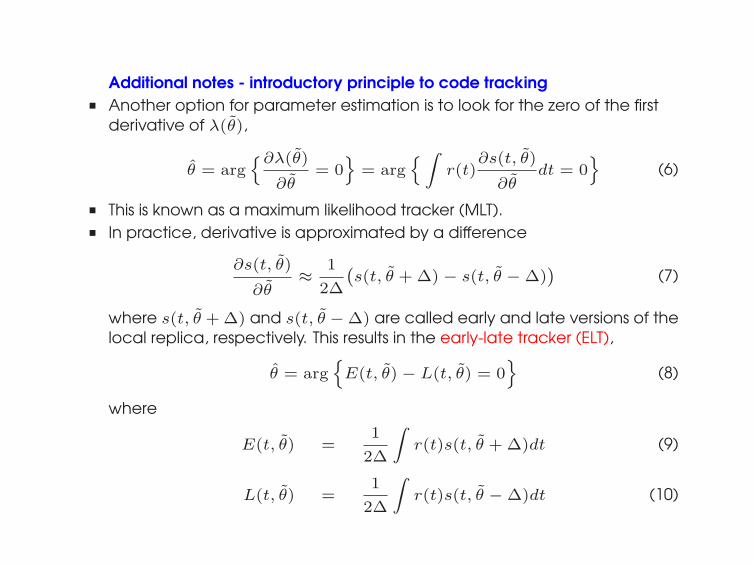
Additional notes - introductory principle to code tracking
■ Another option for parameter estimation is to look for the zero of the first
derivative of λ(θ̃),
θ̂ = argn∂λ(θ̃)
∂θ̃= 0o
= argn
Z
r(t)∂s(t, θ̃)
∂θ̃dt = 0
o
(6)
■ This is known as a maximum likelihood tracker (MLT).
■ In practice, derivative is approximated by a difference
∂s(t, θ̃)
∂θ̃≈ 1
2∆
`
s(t, θ̃ + ∆) − s(t, θ̃ − ∆)´
(7)
where s(t, θ̃ + ∆) and s(t, θ̃ − ∆) are called early and late versions of thelocal replica, respectively. This results in the early-late tracker (ELT),
θ̂ = argn
E(t, θ̃) − L(t, θ̃) = 0o
(8)
where
E(t, θ̃) =1
2∆
Z
r(t)s(t, θ̃ + ∆)dt (9)
L(t, θ̃) =1
2∆
Z
r(t)s(t, θ̃ − ∆)dt (10)

An example - code acquisition
■ Consider the following example of an ”all-one” data sequence (e.g. a
training sequence which helps to achieve correct timing) with a
spreading code signal of period T = NTc.
■ Formally, the transmitted signal at the baseband is
c(t) =∞X
l=−∞clpTc(t − lTc) (11)
where cl’s are the elements of a (periodic) signature sequence.
■ Assuming AWGN channel the received (carrier-modulated) signal is a
delayed copy of the transmitted one corrupted by AWGN noise:
r(t) = c(t − td) cos(2πfct + φ) + n(t) (12)
where fc, φ and td are the carrier frequency, random received phaseand propagation delay, respectively. Without loss of generality, the initial
phase φ will be considered 0 in what follows.
■ The receiver hypothesizes a phase of the spreading sequence to
generate a reference signal
a(t) = c(t − t̂d) cos(2πf̂ct) (13)

resulting in a despreader output (after BPF) equal to
x(t) = c(t − td)c(t − t̂d) cos(2π(f̂c − fc)t) + n′(t) (14)
■ This means that a product signal c(t − td)c(t − t̂d) is at the baseband if
the frequency error f̂c − fc is zero (or small, in practice).
■ In addition, the power of c(t − td)c(t − t̂d) depends solely on the timingerror td − t̂d.
■ Predictably, td − t̂d = 0 results in maximal power to be sensed by theenergy detector.
■ If the energy is detected by amatched filter , we integrate the despread
(product) signal for T seconds and square it. Thus we have a decisionstatistic z:
z =1
T2
˛
˛
˛
˛
Z
Tc(t − td)c(t − t̂d)dt
˛
˛
˛
˛
2
=1
T2|Rc(td − t̂d)|2 (15)
which is thus directly related to the continuous-time periodic
autocorrelation functionRc(τ) of the spreading code.

■ In practice, the continuous range of values of t̂d is not possible
to be treated but some type of range quantization is needed.
■ The resulting candidate values are called cells or bins
resulting in multiple-hypothesis problem: locate the cell which
most likely contain the unknown parameter, given the
observation r(t).
■ This is known as coarse code synchronization or code
acquisition problem.
X Time bins
Frequency bins
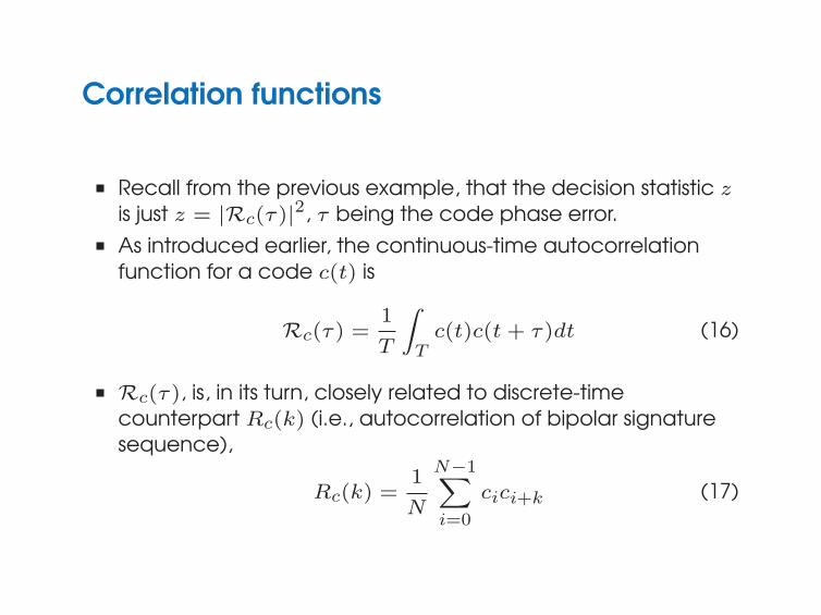
Correlation functions
■ Recall from the previous example, that the decision statistic zis just z = |Rc(τ)|2, τ being the code phase error.
■ As introduced earlier, the continuous-time autocorrelation
function for a code c(t) is
Rc(τ) =1
T
Z
Tc(t)c(t + τ)dt (16)
■ Rc(τ), is, in its turn, closely related to discrete-timecounterpart Rc(k) (i.e., autocorrelation of bipolar signaturesequence),
Rc(k) =1
N
N−1X
i=0
cici+k (17)
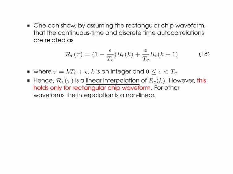
■ One can show, by assuming the rectangular chip waveform,
that the continuous-time and discrete time autocorrelations
are related as
Rc(τ) = (1 − ǫ
Tc)Rc(k) +
ǫ
TcRc(k + 1) (18)
■ where τ = kTc + ǫ, k is an integer and 0 ≤ ǫ < Tc
■ Hence,Rc(τ) is a linear interpolation of Rc(k). However, thisholds only for rectangular chip waveform. For other
waveforms the interpolation is a non-linear.

■ For example, for m-sequences Rc(k) = −1/N for all k 6= 0and Rc(0) = 1. The resulting continuous-time autocorrelationhence equals (T = NTc)
Rc(τ) =
(
1 − N+1N
|τ |Tc
for |τ | < Tc
− 1N for |τ | > Tc
(19)
−15 −10 −5 0 5 10 15−0.2
0
0.2
0.4
0.6
0.8
1
1.2

■ Considering the decision statistic
z = |Rc(τ)|2 = |Rc(td − t̂d)|2 we should thus set a thresholdvalue γ for our decision:
if z ≥ γ then t̂d is declared as a ”correct timing” (20)
if z < γ then t̂d is declared as a ”incorrect timing” (21)
■ Finding a suitable value γ is know as a threshold settingproblem.
■ For example, in ideal channel (where the received signal is
just a delayed copy), if we are targeting to an accuracy
±Tc/2, we should choose γ = (N−12N )2. This is just the value for
z if the received and reference codes would be misalignedexactly Tc/2 sec.

Acquisition in noise: detection probability
■ The probability of detection is the probability that the test
statistic is higher than the chosen threshold, under the correct
code phase hypothesis:
Pd = Proba(z ≥ γ| − Tc < τ < Tc) (22)
■ Threshold-dependent
■ Typically, it is computed at a certain false alarm probability

Acquisition in noise: false alarms and misses
■ The presence of noise causes two different kinds of errors in
the acquisition process
⋆ A false alarm occurs when the decision statistic exceedsthe threshold for an incorrect hypothesized phase
⋆ A miss or miss-detection occurs when the decision statisticfalls below the threshold for a correct hypothesized phase.
■ A false alarm will cause an incorrect phase to be passed to
the code tracking loop which, as a consequence, will not be
able to lock on to the DS-SS signal.
■ Eventually, acquisition mode is activated again, resulting in
severe time penalty to the overall acquisition time.
■ On the other hand, a miss will cause the acquisition circuitry
to neglect the current correct hypothesized phase.

■ Therefore a correct acquisition will not be achieved until the
next correct hypothesized phase comes around.
■ Hence, the time penalty of a miss depends on acquisition
strategy.
■ In general, we would like to design the acquisition circuitry to
minimize both the false alarm and miss probabilities (Pfa and
Pm, respectively) by e.g. properly selecting the decision
threshold.
■ These probabilities can mostly be explained by the
⋆ dwell time, that is, the time needed to evaluate a singlehypothesized phase of the spreading code
⋆ complexity of the acquisition circuitry⋆ interference reduction capability of acquisition method

■ Two major design approaches
⋆ minimize the overall acquisition time given tolerances tofalse alarm and miss probabilities
⋆ minimize the overall acquisition time by associatingpenalty times with false alarms and misses.
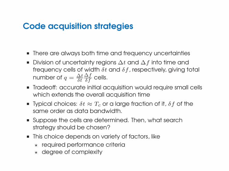
Code acquisition strategies
■ There are always both time and frequency uncertainties
■ Division of uncertainty regions∆t and∆f into time andfrequency cells of width δt and δf , respectively, giving total
number of q = ∆tδt
∆fδf cells.
■ Tradeoff: accurate initial acquisition would require small cells
which extends the overall acquisition time
■ Typical choices: δt ≈ Tc or a large fraction of it, δf of thesame order as data bandwidth.
■ Suppose the cells are determined. Then, what search
strategy should be chosen?
■ This choice depends on variety of factors, like
⋆ required performance criteria⋆ degree of complexity

⋆ computational power available⋆ prior available information about the location of a correctcell
■ Search strategies:
● parallel● serial● hybrid
■ Detection strategies:
● single-dwell● multi-dwell

Parallel search
■ Brute-force approach: create a bank of parallel correlation
branches for cell. This is called a fully parallel search.
■ However, practical implementation quickly becomes
unreasonable and perhaps impossible, because of the need
of a high number of correlators.
■ Parallel search is feasible for small uncertainty regions, or as a
nested search strategy within another search strategy (e.g.
hybrid serial/parallel -type search)

Serial search
■ In serial search the acquisition circuit attempts to cycle
through and test all possible phases one by one (serially)
■ The circuit complexity for serial search is low. However,
penalty time associated with a miss is large, since the correct
acquisition will not be achieved until the next correct
hypothesized phase comes around.
■ Therefore, a larger dwell time is needed to reduce the miss
probability.
■ This, together with the serial searching nature, gives a large
overall acquisition time (i.e., slow acquisition).

Single-dwell versus Multi-dwell search
■ In serial search (or generally in acquisition) the penalty time
associated with a false alarm is large. Thus, the decision
threshold γ is set to a high value to make the false alarmprobability small.
■ However, if the threshold is a high value, even the correct cell
is harder to be found. This requires us to increase the dwell
time to reduce the miss probability, since the penalty time
associated with a miss is large, too.
■ As a result, the overall acquisition time needed for the serial
search is inherently large. This is a major limitation of using a
single detection stage.

■ An alternative approach to reduce the overall acquisition
time is to employ a two-stage detection (so called
double-dwell acquisition) scheme
⋆ The first detection stage is designed to have a lowthreshold and a short integration time such that the miss
probability is small but the false alarm probability is high
⋆ The second stage is designed to have small miss and falsealarm probabilities. In this stage only the most probable
cells (from the first stage) are tested.
■ With this configuration, the first stage can reject incorrect
phases rapidly and second stage, which is entered
occasionally, verifies the decisions made by the first stage to
reduce the false alarm probability.
■ By properly choosing the dwell times and decision thresholds
in the two detection stages, the overall acquisition time can
be significantly reduced.
■ In general, multiple stages can be used, resulting in
multi-dwell search.

Reject code phase
"miss""miss"
"hit"Dwell time #1mode
Enter trackingThreshold #2Dwell time #2
Detection: stage #2
"hit"
Detection: stage #1
Threshold #1Select code phase
for evaluation
Figure 1: Typical logic flow diagram for two-dwell (in
general, multi-dwell) detector

Mean acquisition time for serial search
■ As mentioned earlier, one approach of initial acquisition
design is to associate penalty times with false alarms and
misses, and then, try to minimize the overall acquisition time,
Tacq.
■ Since acquisition is a random process, it is a reasonable to
minimize the mean overall acquisition time T̄acq = E[Tacq].
■ In the following we present a simple calculation of the mean
overall acquisition time of a serial search circuit.
■ Here the mean acquisition time is calculated in a
straightforward manner by considering all possible sequences
of events leading to a correct acquisition. Hence the name
direct method.
■ Alternative method for mean acquisition time analysis is the
use of signal flow graph method, which is not considered.

Definitions
■ Let us assume that we cycle through and test a total of Ndifferent hypothesized (equi-probable) phases in each search
cycle until the correct phase is detected.
■ Assume that a penalty time of Tfa seconds is associated with
a false alarm. (Tfa is assumed much greater than a dwell
time Td)
■ The penalty time associated with a miss is NTd, since if we
encounter a miss, the correct phase cannot be detected
until the next cycle.
■ Suppose that:
⋆ the correct phase is in the nth hypothesized position⋆ there are j misses, and⋆ there are k false alarms
■ This results in the overall acquisition time equal to
Tacq(n, j, k) = nTd + jNTd + kTfa (23)

■ Denote Pd and Pfa the probability of detection and false
alarm, respectively. Recall that Pd = 1 − Prob(miss).
Derivation of mean acquisition time
■ Considering the setting just described we notice the following
⋆ number of hypotheses tested equals n + jN⋆ number of correct hypotheses tested equals j + 1⋆ number of incorrect hypotheses tested equals
K∆= n + jN − j − 1
■ Consequently, the overallmean acquisition time equals
T̄acq =NX
n=1
∞X
j=0
KX
k=0
Tacq(n, j, k)P (n, j, k) (24)
where P (n, j, k) denotes the probability for the event(n, j, k) to happen.

■ After (rather) straightforward manipulations mean acquisition
time simplifies to
T̄acq = (N − 1)2 − Pd
2Pd(Td + PfaTfa) +
Td
Pd(25)
■ For example, given Pd = 1 and Pfa = 0 we have
T̄acq = N+12 Td.
■ Recall that both the probabilities Pd and Pfa are functions of
the threshold γ and the used acquisition algorithm itself. Tfaon the other hand depends on the ability to recognize a
falsely chosen phase (verification mode)

Example
■ Recall that one of the goal in the SS system design is to
minimize the overall mean acquisition time.
■ Due to penalty times it is not correct to assume that Pd ≈ 1and Pfa ≈ 0 would result in the minimum time acquisitiontime, see the example below.
0 10 20 30 40 50 60 70 80 90 1000
0.1
0.2
0.3
0.4
0.5
0.6
0.7
0.8
0.9
1
dwell time
Probability of detection
Probability of false alarm
0 10 20 30 40 50 60 70 80 90 100500
1000
1500
2000
2500
3000
dwell time
Mean acquisition time

Code tracking
■ The purpose of code tracking is to perform and maintain fine
synchronization.
■ A code tracking loop starts its operation only after initial
acquisition has been achieved. Hence, we can assume that
we are off by small amounts in both frequency and code
phase.
■ A common fine synchronization strategy is to design a code
tracking circuitry which can track the code phase in the
presence of a small frequency error.
■ After the correct code phase is acquired by the code
tracking circuitry, a standard phase lock loop (PLL) can be
employed to track the carrier frequency and phase.

Early-late gate DLL
■ The idea in early-late gate DLL is to despread the received SS signal r(t)with two spreading signals, which are slightly advanced and retarded in
phase (recall that finding the maximum of the likelihood function is
equivalent with finding the zero crossings of its first derivative)
■ The two local reference signals are
c+
(t) = c(t − t̂d +∆
2Tc)
c−
(t) = c(t − t̂d − ∆
2Tc)
where t̂d is the initial estimate for the phase of the spreading code(acquisition stage)
■ Suppose for a moment that the received signal is just a delayed copy, i.e.
r(t) = c(t − td). Let’s look at the despreader output when c+(t) and
c−(t) are employed.
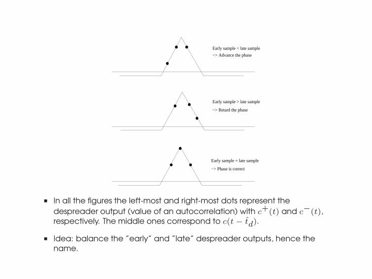
Early sample = late sample
−> Phase is correct
Early sample > late sample
−> Retard the phase
−> Advance the phase
Early sample < late sample
■ In all the figures the left-most and right-most dots represent the
despreader output (value of an autocorrelation) with c+(t) and c−(t),respectively. The middle ones correspond to c(t − t̂d).
■ Idea: balance the ”early” and ”late” despreader outputs, hence the
name.

X
X LPF
LPF ( )
( )2
2
++
−Loop filter
VCOSpreading codegenerator
■ Balancing is achieved by the loop filter and Voltage Controlled Oscillator
(VCO). In digital DLLs, VCO is replaced by a Numerically Controlled
Oscillator (NCO).
■ Basically, the loop filter outputs the DC component of its input (that is,
difference between the early and late despreader outputs), which
controls the output phase of VCO.
■ Formally, consider (for simplicity) a constant envelope data b(t) (e.g.BPSK) and let us neglect the presence of noise. The received signal r(t) in
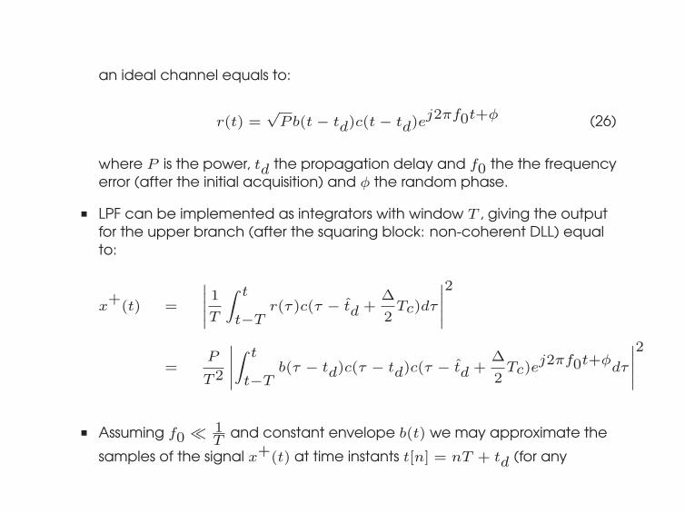
an ideal channel equals to:
r(t) =√
Pb(t − td)c(t − td)ej2πf0t+φ
(26)
where P is the power, td the propagation delay and f0 the the frequencyerror (after the initial acquisition) and φ the random phase.
■ LPF can be implemented as integrators with window T , giving the outputfor the upper branch (after the squaring block: non-coherent DLL) equal
to:
x+
(t) =
˛
˛
˛
˛
˛
1
T
Z t
t−Tr(τ)c(τ − t̂d +
∆
2Tc)dτ
˛
˛
˛
˛
˛
2
=P
T2
˛
˛
˛
˛
˛
Z t
t−Tb(τ − td)c(τ − td)c(τ − t̂d +
∆
2Tc)e
j2πf0t+φdτ
˛
˛
˛
˛
˛
2
■ Assuming f0 ≪ 1Tand constant envelope b(t) we may approximate the
samples of the signal x+(t) at time instants t[n] = nT + td (for any

integer n) as
x+
(t[n]) ≈ P
T2
˛
˛
˛
˛
˛
Z t[n]
t[n]−Tc(τ − td)c(τ − t̂d +
∆
2Tc)
˛
˛
˛
˛
˛
2
= P
˛
˛
˛
˛
Rc(td − t̂d +∆
2Tc)
˛
˛
˛
˛
2(27)
■ Similarly, x−(t[n]) ≈ P˛
˛
˛Rc(td − t̂d − ∆2 Tc)
˛
˛
˛
2
■ The difference signal x−(t) − x+(t) is the passed through loop filter whichbasically outputs the mean value of its input. Thus, the error signal
approximately equals
ǫ(t̂d) ≈ P
˛
˛
˛
˛
Rc(td − t̂d − ∆
2Tc)
˛
˛
˛
˛
2−˛
˛
˛
˛
Rc(td − t̂d +∆
2Tc)
˛
˛
˛
˛
2!
= P S∆
“td − t̂dTc
”
(28)
where
S∆(u) = Rc“
(u − ∆
2)Tc”2
− Rc“
(u +∆
2)Tc”2
(29)

is so-called S-curve of a DLL.
■ S-curve presents the error signal as a function of code phase mismatch.
The correct code phase is found in the zero-crossing from above (if early
minus late) or from below (if late minus early, as in the example above) of
the S-curve.
■ In the above example, non-coherent S-curve is considered.
■ S-curves depend on∆ = the early-late spacing.

Example of S-curve in infinite bandwidth, single path
■ Typical non-coherent S-curves for different values∆ of early-late spacing.
■ From the figure we see, that if we choose∆ = 1 chip or smaller, the loopfilter output ǫ(t) will be linear with respect to the code phaseerror/channel delay error td − t̂d, if td − t̂d ≤ ∆Tc/2 (e.g., to 0.5 for∆ = 1). Hence, we can use the loop filter output to drive the VCO, whichadjusts the hypothesized phase reference t̂d to achieve finesynchronization.
−2 −1.5 −1 −0.5 0 0.5 1 1.5 2−1
−0.8
−0.6
−0.4
−0.2
0
0.2
0.4
0.6
0.8
1Normalized S curves for non−coherent DLL
Channel delay error [chips]
S−c
urve
∆=2 chips
−2 −1.5 −1 −0.5 0 0.5 1 1.5 2−1
−0.8
−0.6
−0.4
−0.2
0
0.2
0.4
0.6
0.8
1Normalized S curves for non−coherent DLL
Channel delay error [chips]
S−c
urve
∆=1 chips
−2 −1.5 −1 −0.5 0 0.5 1 1.5 2−1
−0.8
−0.6
−0.4
−0.2
0
0.2
0.4
0.6
0.8
1Normalized S curves for non−coherent DLL
Channel delay error [chips]
S−c
urve
∆=0.5 chips
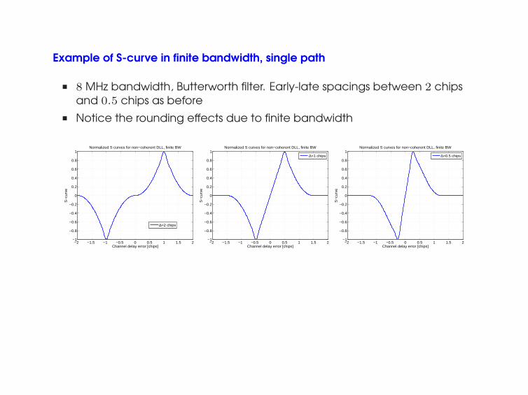
Example of S-curve in finite bandwidth, single path
■ 8 MHz bandwidth, Butterworth filter. Early-late spacings between 2 chipsand 0.5 chips as before
■ Notice the rounding effects due to finite bandwidth
−2 −1.5 −1 −0.5 0 0.5 1 1.5 2−1
−0.8
−0.6
−0.4
−0.2
0
0.2
0.4
0.6
0.8
1Normalized S curves for non−coherent DLL, finite BW
Channel delay error [chips]
S−c
urve
∆=2 chips
−2 −1.5 −1 −0.5 0 0.5 1 1.5 2−1
−0.8
−0.6
−0.4
−0.2
0
0.2
0.4
0.6
0.8
1Normalized S curves for non−coherent DLL, finite BW
Channel delay error [chips]
S−c
urve
∆=1 chips
−2 −1.5 −1 −0.5 0 0.5 1 1.5 2−1
−0.8
−0.6
−0.4
−0.2
0
0.2
0.4
0.6
0.8
1Normalized S curves for non−coherent DLL, finite BW
Channel delay error [chips]
S−c
urve
∆=0.5 chips

Multipath effect
■ Infinite bandwidth; two equal paths at 0.5 chips distance from each other.
■ Notice the multipath merging effect⇒ the zero-crossing occurs at
incorrect delay
−2 −1.5 −1 −0.5 0 0.5 1 1.5 2−1
−0.8
−0.6
−0.4
−0.2
0
0.2
0.4
0.6
0.8
1Normalized S curves for non−coherent DLL, finite BW
Channel delay error [chips]
S−
curv
e
∆=1 chips
−2 −1.5 −1 −0.5 0 0.5 1 1.5 2−1
−0.8
−0.6
−0.4
−0.2
0
0.2
0.4
0.6
0.8
1Normalized S curves for non−coherent DLL, finite BW
Channel delay error [chips]
S−
curv
e
∆=0.5 chips

Other tracking loops
■ In order to cope with multipaths, many enhancements of DLLs have been
proposed: Sample Correlated Choose Largest (SCLL) loops, narrow
correlator, very early-very late (VEVL) loops, Multipath Estimating DLL
(MEDLL), etc.
■ Also alternative feedforward tracking solutions have been studied (e.g.,
directly from ML principle)⇒more correlators needed
■ The topic of accurate code tracking in multipath fading and in the
presence of various interferers (MUI, AWGN, etc) is one of the most
challenging research topics in SS nowadays, for both communication and
navigation applications.

Example: SCCL
■ Chen & Davisson, 1994, M. Latva-aho & al., 1996
■ Proposed for WCDMA systems in order to deal better with multipaths.
Example below: coherent SCCL:
I&D
I&D
I&D
I&D
I&D
I&D
PN codegenerator
NCO+1, 0, -1
late
in-time
early
r(t)maximumtowardsshift
b α^ i i^
bi^ αi^
bi^ αi^
* *
**
* *

Example: VEVL
■ Proposed for Galileo and modernized GPS signals (Betz & al., 1999). Two
extra branches for better dealing with false side peaks (e.g., caused by
multipaths or by modulation type)
I&D on N
c msec
I&D on N
c msec
| | 2
| | 2
+
-
Loop filter NCO
r(t)
late code
early code
| | 2
| | 2 I&D on N c msec
I&D on N c msec
+
- very late code
very early code constant factor
a
+
+

Conclusions
■ Code synchronization is a pre-requisite for any SS receiver
■ It is usually implemented in 2 steps: code acquisition and tracking.
■ In the acquisition part, low mean acquisition times are desirable, as well as
low complexity, high detection probability and low false alarms
■ In the tracking part, the main goals are to track accurately the code
phase (i.e., low time-delay errors) and to preserve a high mean time to
loose lock.
■ The basic tracking structures are the DLLs, but many enhanced variants
exist.