Lecture 3 – Basic Feedbackweb.stanford.edu/.../ee/ee392m/ee392m.1056/Lecture3_BasicFeed… · – The name ‘P’ is used in process industries and in servosystems, less in flight

EE392m - Spring 2005Gorinevsky

Control Engineering 3-1

Lecture 3 – Basic Feedback

Simple control design and analysis • Linear model with feedback control • Use simple model design control validate • Simple P loop with an integrator • Velocity estimation • Time scale • Cascaded control loops



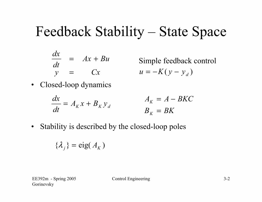
Feedback Stability – State Space

• Closed-loop dynamics

• Stability is described by the closed-loop poles

Cxy

BuAxdtdx

=

+=)( dyyKu −−=

BKCAAK −=

Simple feedback control

dKK yBxAdtdx +=

)eig(}{ Kj A=λ

BKBK =



Closed-loop eigenvalues

• Roots = poles = eigenvalues

• Can be plotted for different gains K

• Root locus plot

F16 Longitudinal Model Example

[ ]03.5700

18.00

1015.217.0

08.1082.01095.2100091.0002.11054.248.02.3282.81093.1

3

12

4

2

=

⎥⎥⎥⎥

⎦

⎤

⎢⎢⎢⎢

⎣

⎡

−

⋅−=

⎥⎥⎥⎥

⎦

⎤

⎢⎢⎢⎢

⎣

⎡

⋅

−⋅−−−⋅−

=−

−

−

−

C

BA

)(eig BKCA −

% Take A from % the F16 example>> eig(A)

ans =-1.9125 -0.1519 + 0.1143i-0.1519 - 0.1143i0.0970

% Closed-loop poles >> K = -0.2;>> eig(A-B*K*C)

ans =-1.4419 -0.0185 -0.3294 + 1.1694i-0.3294 - 1.1694i



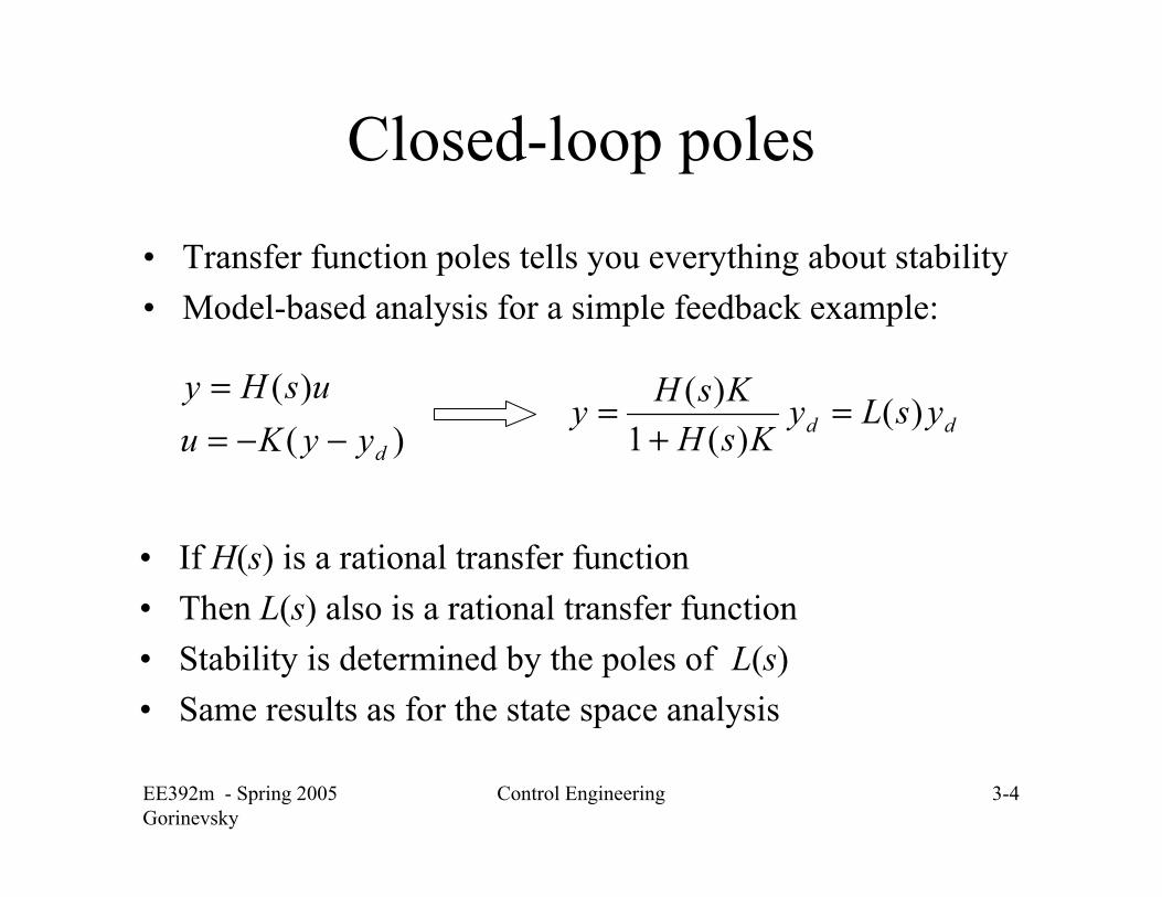
Closed-loop poles

• Transfer function poles tells you everything about stability• Model-based analysis for a simple feedback example:

)()(

dyyKuusHy−−=

=dd ysLy

KsHKsHy )()(1

)( =+

=

• If H(s) is a rational transfer function • Then L(s) also is a rational transfer function • Stability is determined by the poles of L(s) • Same results as for the state space analysis



Control of a 1st order system

• Simplest dynamics, 1st order system • Simple feedback works just fine

– Static output feedback is sometimes called P control– P = ‘proportional’– The name ‘P’ is used in process industries and in servosystems,

less in flight control

• Closed-loop dynamics are very well understood • Can be used as a design template for more complex

systems, cascade loops



Control of a 1st order system

• First order system, integrator dynamics

• P Control

• Closed loop dynamics

• Eigenvalue=pole

xy

buxdtdx

⋅=

+⋅=

1

0

1

0

===

CbB

A

)( dyykbdtdx −−=

kb−=λ

)( dyyku −−=



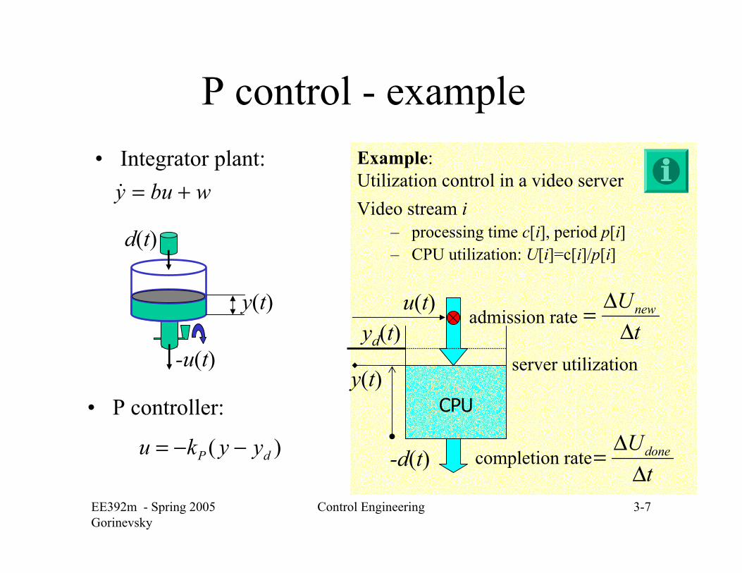
Example: Utilization control in a video server

P control - example• Integrator plant:

wbuy +=&

)( dP yyku −−=

• P controller:

admission rate

CPU

u(t)

completion rate

server utilization-u(t)

y(t)

d(t)

y(t)

yd(t)

-d(t)

Video stream i– processing time c[i], period p[i]– CPU utilization: U[i]=c[i]/p[i]

tUnew

∆∆=

tUdone

∆∆=



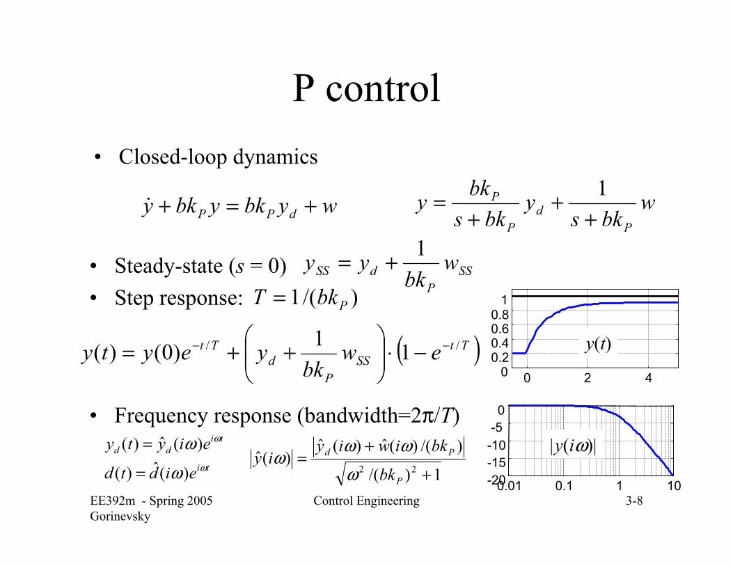
P control• Closed-loop dynamics

wbks

ybks

bkyP

dP

P

++

+= 1

wybkybky dPP +=+&

• Steady-state (s = 0)• Step response:

• Frequency response (bandwidth=2π/T)

SSP

dSS wbk

yy 1+=

( )TtSS

Pd

Tt ewbk

yeyty // 11)0()( −− −⋅⎟⎟⎠

⎞⎜⎜⎝

⎛++=

1)/(

)/()(ˆ)(ˆ)(ˆ

22 +

+=

P

Pd

bk

bkiwiyiy

ωωω

ω0.01 0.1 1 10-20

-15-10-5 0

0 2 400.20.40.60.8

1

y(t)

|y(iω)|ti

tidd

eidtd

eiytyω

ω

ω

ω

)(ˆ)(

)(ˆ)(

=

=

)/(1 PbkT =



Control and Error Peaking• Fast poles are not necessarily good• This might mean large peak resonse• Example: P control of an integrator

( )tbkbkth PP −= exp)(

0

slow response

fast response

• Engineering design is a series of tradeoffs

dyhy *= - closed-loop impulse response

dP yhku *= - control impulse response



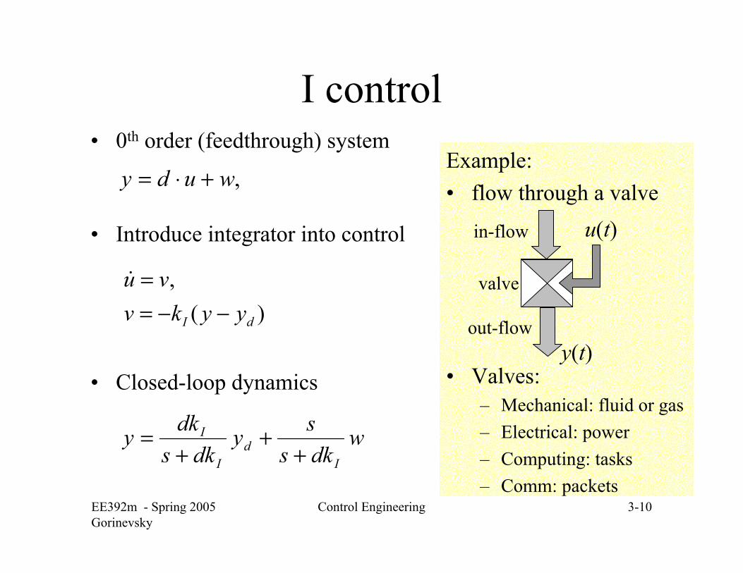
Example:• flow through a valve

• Valves:– Mechanical: fluid or gas– Electrical: power– Computing: tasks– Comm: packets

I control

• Introduce integrator into control

• Closed-loop dynamics

)(,

dI yykvvu

−−==&

,wudy +⋅=

wdkssy

dksdky

Id

I

I

++

+=

y(t)

u(t)in-flow

out-flow

valve

• 0th order (feedthrough) system



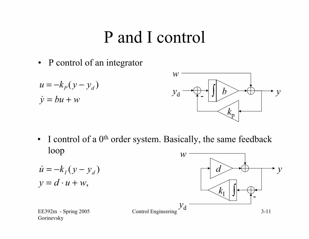
P and I control• P control of an integrator

• I control of a 0th order system. Basically, the same feedback loop

wbuy +=&)( dP yyku −−=

d

kI ∫ -yd

wy)( dI yyku −−=&

,wudy +⋅=

kp

b∫-yd

w

y



First order estimation - differentiator

• Differentiating filter• Velocity estimation: y v

• Observer

• Velocity estimation filter

xy

vdtdx

=

=

xy

yyLdtxd

ˆˆ

)ˆ(ˆ

=

−= )ˆ(ˆˆ yyL

dtxdv −==

xsL

sv 11ˆ −+

=L

1∫ -y

y

v

Model:



First order estimation – example

InputSignal

Feedback gainL = 2

OutputSignal

ysL

sv 11ˆ −+

=

0 1 2 3 4 5 6 7 8 9 10-1

0

1

2

3

4

5INPUT SIGNAL y

0 1 2 3 4 5 6 7 8 9 10

-1

-0.5

0

0.5

1

TIME

ESTIMATED DERIVATIVE v


Control Engineering 3-14 Val

idat

ion

an

d ve

rifi

cati

onD

esig

n a

nd

anal

ysis

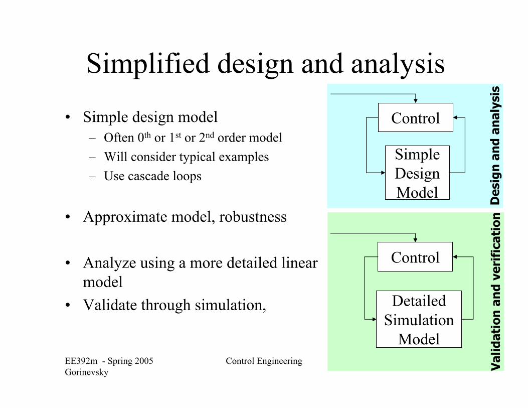
Simplified design and analysis

• Simple design model– Often 0th or 1st or 2nd order model – Will consider typical examples– Use cascade loops

• Approximate model, robustness

• Analyze using a more detailed linear model

• Validate through simulation,

Control

Simple Design Model

Control

Detailed Simulation

Model



Example

e

e-

.q..qq

.q..V

δαθ

δαα

180081 820

101529100210

3

−−==

⋅−+−==

&

&

&

[ ] xy

uxdtdx

C

BA

⋅=

⋅⎥⎥⎥

⎦

⎤

⎢⎢⎢

⎣

⎡

−

⋅−+⋅

⎥⎥⎥

⎦

⎤

⎢⎢⎢

⎣

⎡

−

−=

−

4434421

4434421444 3444 21

03.570

18.00

1015.2

08.1082.010091.0002.1 3

>> eig(A)ans =

0-0.1880-1.9120

z

x

δe

α θV

eu δ=

θ3.57=y

• F16 longitudinal model, constant velocity• Assume that the velocity is maintained by regulating thrust



F16 Attitude Control• Simulated step response• At slow time scale, the integrator dynamics are dominant• Approximate by a simple integrator model

0 2 4 6 8 10 12

-200

-150

-100

-50

0

TIME (s)

STEP RESPONSE

edtd δθ 02−=



Simple model

‘Detailed’ model

F16 Attitude Control• P control design for an integrator

• Time responses for the simple model and for the ‘detailed’ model

)( dPe k θθδ −=

edtd δθ 02−=

dθ

005.0=Pk

)( dPe k θθδ −=

CxBAxx e

=+=

θδ&

dθ

10)20/(1 == PkT

0 10 20 30 40 50 600

0.2

0.4

0.6

0.8

1

1.2

1.4

TIME (s)

STEP RESPONSE



Time scale • The same plot at different scales • Bandwidth 1/Timescale

• Simple 2nd order model example: H(s) = 1/(1+s+s2)

0 0.5 10

0.1

0.2

0.3

0.4

0 5 100

0.5

1

1.5

0 50 1000

0.5

1

1.5H ≈ 1/s2 H = 1/(1+s+s2) H ≈ 1Fast Intermediate Slow Time scales:



Time Scale and Frequency Response

Frequency response for the example:

H(s) = 1/(1+s+s2)

Bandwidth=1/Timescale

• The bandwidth is limited by model uncertainty: Lectures 9-10

-80

-60

-40

-20

0

20

Mag

nitu

de (

dB)

10-2

10-1

100

101

102

-180

-135

-90

-45

0

Pha

se (d

eg)

Bode Diagram

Frequency (rad/sec)

0 0.5 10

0.1

0.2

0.3

0.4

0 5 100

0.5

1

1.5

0 50 1000

0.5

1

1.5

Fast

Slow

Time scales:

Intermediate



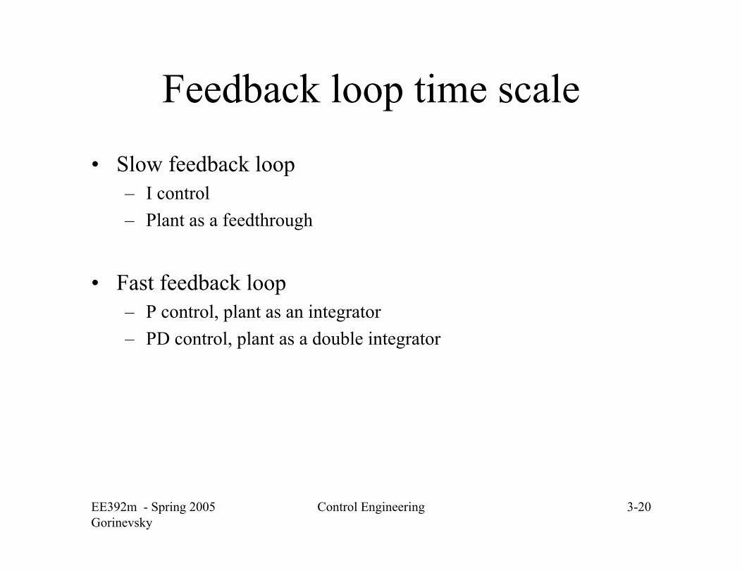
Feedback loop time scale

• Slow feedback loop– I control– Plant as a feedthrough

• Fast feedback loop– P control, plant as an integrator– PD control, plant as a double integrator



Cascaded loop design• Inner loop has faster time scale than outer loop • In the outer loop time scale, consider the inner loop as

a 0th or 1st order system that follows its setpoint input

inner loop

-inner loop

setpoint

output

Plant

Inner Loop Control

Outer Loop Control

-

outer loop

setpoint



Servomotor Speed Control Example

• The control goal is to track a velocity setpoint

• Mechanical time constant TJ is dominant.

• Use simple model

model

usTsT

GyIJ )1)(1( ++

=

Transfer function

sec02.0sec,1.0 == IJ TT

MotorPower amp sensor

speed vcontrolvoltage u

setpoint vd

controller -

uTG

sy

J

⋅= 1

vy =duRIILcIbvvJ

=+=+

&

&

1=G



0 0.05 0.1 0.15 0.2 0.25 0.3 0.35 0.40

0.2

0.4

0.6

0.8

1

OPEN LOOP STEP RESPONSE y

0 0.05 0.1 0.15 0.2 0.25 0.3 0.35 0.40

0.2

0.4

0.6

0.8

1

CLOSED LOOP STEP RESPONSE

Servomotor Example, cont’d

• Design P control for the simple model uTG

sv

J

⋅= 1)( dV vvku −−=


Simplified model

01.0/

110

=⋅

=

=

JPloop

V

TGkT

k



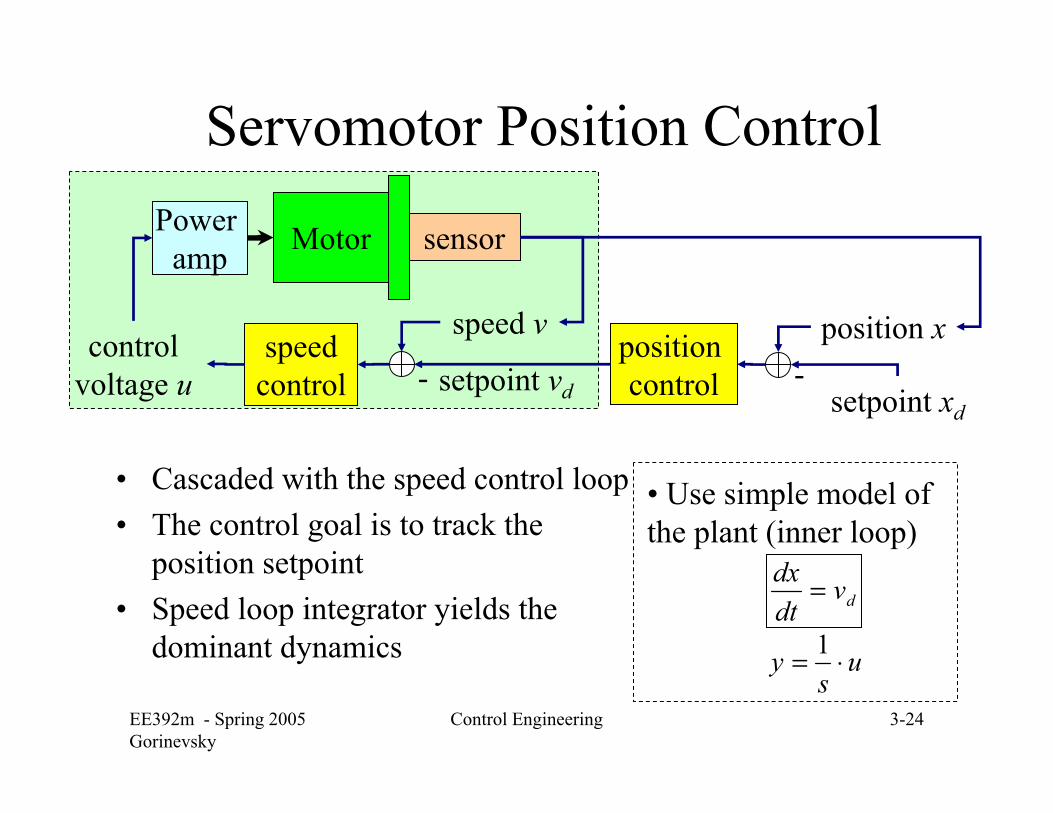
Servomotor Position Control

• Cascaded with the speed control loop • The control goal is to track the

position setpoint• Speed loop integrator yields the

dominant dynamics dv

dtdx =

• Use simple model of the plant (inner loop)

MotorPower amp sensor

position xcontrolvoltage u setpoint vd

speedcontrol -

us

y ⋅= 1

speed v

setpoint xd

position control -



Servomotor Position, cont’d

• Design P control for the simple model dvs

y ⋅= 1)( dPd yykv −−=

0 0.05 0.1 0.15 0.2 0.25 0.3 0.35 0.40

0.1

0.2

0.3

0.4

0.5STEP RESPONSE OF POSTION y WITH OUTER LOOP OPEN

0 0.05 0.1 0.15 0.2 0.25 0.3 0.35 0.40

0.2

0.4

0.6

0.8

1

CLOSED LOOP STEP RESPONSE


Simplified model

05.01

120

=⋅

=

=

Ploop

P

kT

k



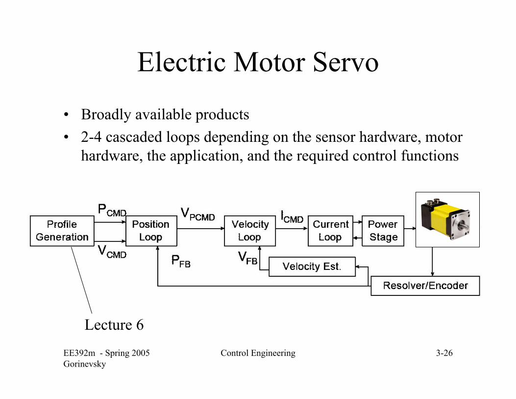
Electric Motor Servo

• Broadly available products• 2-4 cascaded loops depending on the sensor hardware, motor

hardware, the application, and the required control functions

Lecture 6



Aircraft Cascaded Loops

• In practice, multivarable control design might be done for attitude control

• Otherwise, aircraft is represented as a chain of several integrators



Flight Control

Guidance and Autopilot

FMS/MMS

Basic cascaded loops in aircraft

Actuator servos

Angular rate

Angular position; Attitude

Translational velocity

Translational position

WaypointAltitude, coordinates

Commanded airspeed

Angular rate command

Elevator positionFlight ActuatorsActuators

Attitude command

x

α θ V



Aircraft Cascaded LoopsEmbeded servo avionics• Actuators, 100 hz bandwidth

Flight Control box• Angular rate, 2Hz bandwidth• Angular position, 0.5Hz bandwidth

Autopilot/Guidance • Translational velocity, 5 sec• Translational position, 30 sec

FMS - Flight Management System• Waypoint, 100-1000 sec



• Descent/Abort Guidance

• Dale Enns, Honeywell, 1989/1997

X-38 - Space Station Lifeboat

Cascaded Loop Example

Documents

Lecture 3 – Basic Feedbackweb.stanford.edu/.../ee/ee392m/ee392m.1056/Lecture3_BasicFeed… · – The name ‘P’ is used in process industries and in servosystems, less in flight