Embed Size (px)
Citation preview
EE392m - Spring 2005Gorinevsky
Control Engineering 5-1
Lecture 5 –Sampled Time Control
• Sampled time vs. continuous time: implementation, aliasing
• Linear sampled systems modeling refresher, DSP• Sampled-time frequency analysis • Sampled-time implementation of the basic controllers
– I, PI, PD, PID – 80% (or more) of control loops in industry are digital PID
EE392m - Spring 2005Gorinevsky
Control Engineering 5-2
),,(),,()(
tuxgytuxfdtx
==+
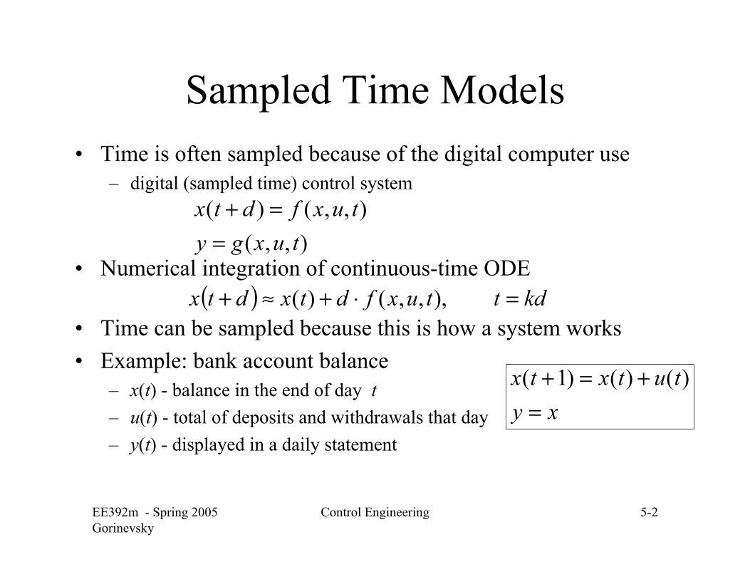
Sampled Time Models • Time is often sampled because of the digital computer use
– digital (sampled time) control system
• Numerical integration of continuous-time ODE
• Time can be sampled because this is how a system works• Example: bank account balance
– x(t) - balance in the end of day t– u(t) - total of deposits and withdrawals that day– y(t) - displayed in a daily statement
( ) kdttuxfdtxdtx =⋅+≈+ ),,,()(
xytutxtx
=+=+ )()()1(
EE392m - Spring 2005Gorinevsky
Control Engineering 5-3
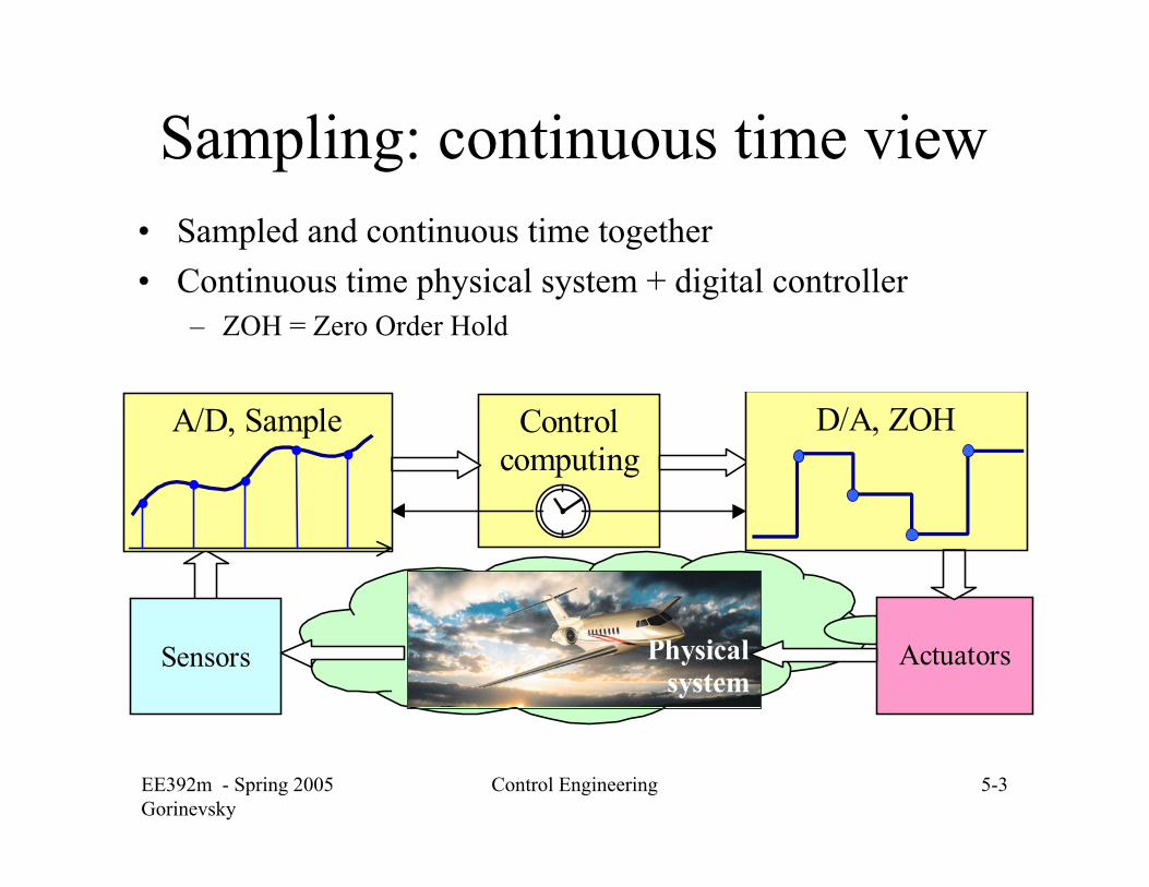
Sampling: continuous time view• Sampled and continuous time together• Continuous time physical system + digital controller
– ZOH = Zero Order Hold
Sensors
Controlcomputing
ActuatorsPhysicalsystem
D/A, ZOHA/D, Sample
EE392m - Spring 2005Gorinevsky
Control Engineering 5-4
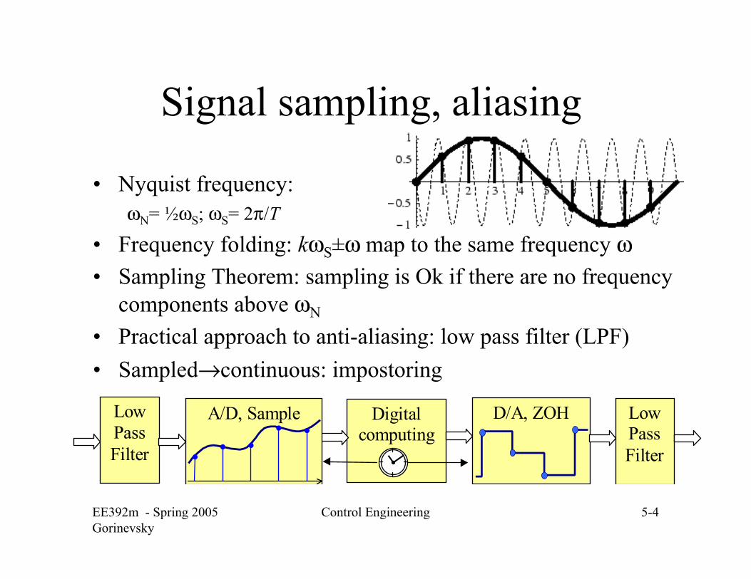
Signal sampling, aliasing
• Nyquist frequency: ωN= ½ωS; ωS= 2π/T
• Frequency folding: kωS±ω map to the same frequency ω• Sampling Theorem: sampling is Ok if there are no frequency
components above ωN
• Practical approach to anti-aliasing: low pass filter (LPF) • Sampled→continuous: impostoring
Digitalcomputing
D/A, ZOHA/D, SampleLowPassFilter
LowPassFilter
EE392m - Spring 2005Gorinevsky
Control Engineering 5-5
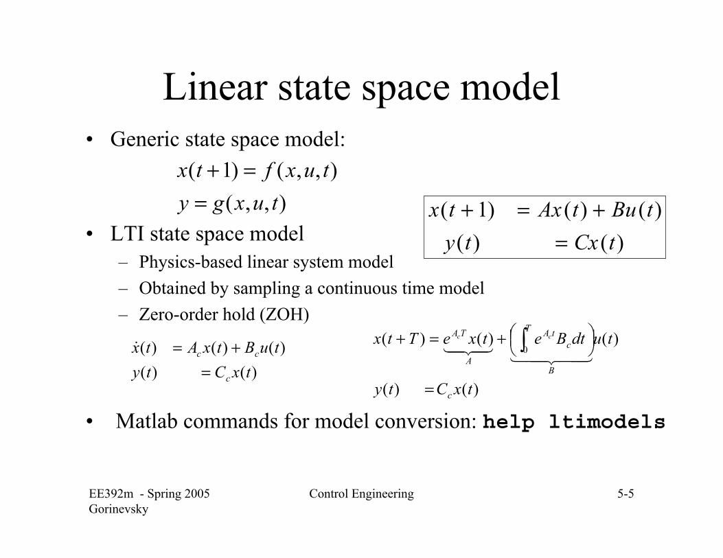
Linear state space model • Generic state space model:
• LTI state space model– Physics-based linear system model– Obtained by sampling a continuous time model– Zero-order hold (ZOH)
• Matlab commands for model conversion: help ltimodels
)()()()()1(
tCxtytButAxtx
=+=+),,(
),,()1(tuxgy
tuxftx=
=+
)()()()()(
txCtytuBtxAtx
c
cc
=+=&
)()(
)()()(0
txCty
tudtBetxeTtx
c
B
c
T tA
A
TA cc
=
⎟⎠⎞⎜
⎝⎛+=+ ∫
443442143421
EE392m - Spring 2005Gorinevsky
Control Engineering 5-6
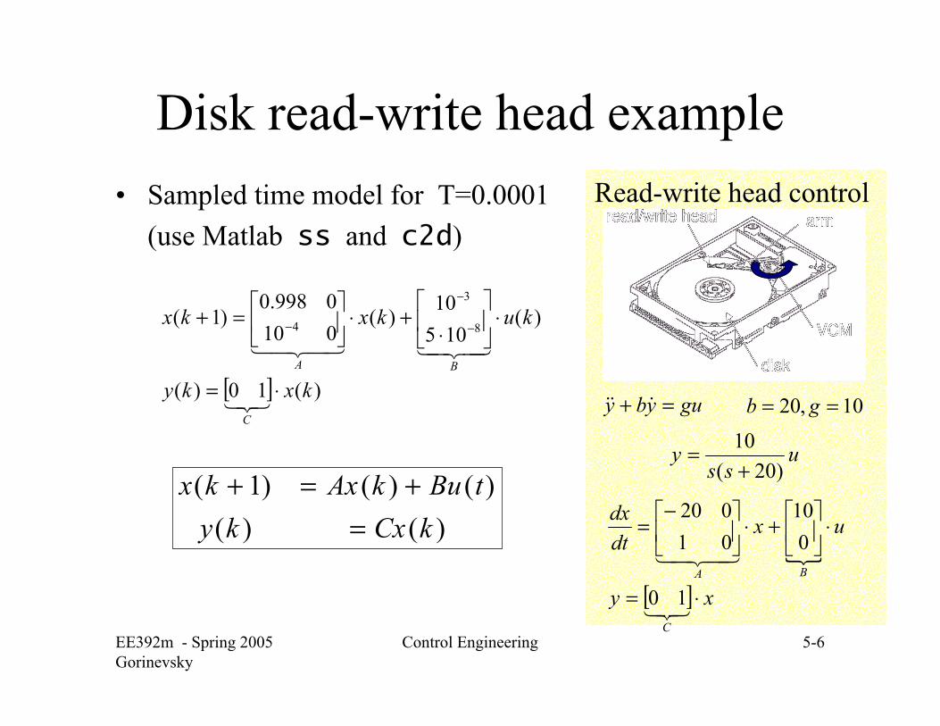
Read-write head control
Disk read-write head example• Sampled time model for T=0.0001
(use Matlab ss and c2d)
guyby =+ &&&
uss
y)20(
10+
=
{
[ ] xy
uxdtdx
C
BA
⋅=
⋅⎥⎦
⎤⎢⎣
⎡+⋅⎥⎦
⎤⎢⎣
⎡−=
321
43421
10
010
01020
10,20 == gb[ ] )(10)(
)(105
10)(
0100998.0
)1( 8
3
4
kxky
kukxkx
C
BA
⋅=
⋅⎥⎦
⎤⎢⎣
⎡
⋅+⋅⎥
⎦
⎤⎢⎣
⎡=+−
−
−
321
4342143421
)()()()()1(
kCxkytBukAxkx
=+=+
EE392m - Spring 2005Gorinevsky
Control Engineering 5-7
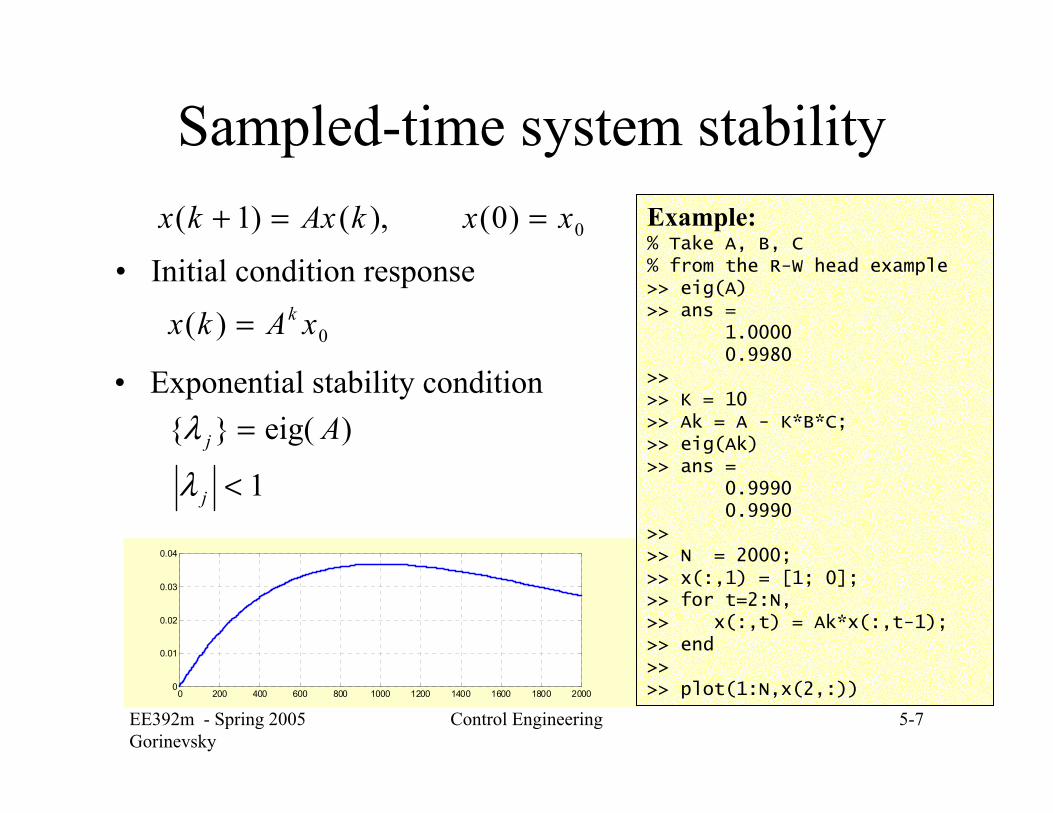
Sampled-time system stability
• Initial condition response0)0(),()1( xxkAxkx ==+
0)( xAkx k=
Example: % Take A, B, C % from the R-W head example>> eig(A)>> ans =
1.0000 0.9980
>>>> K = 10>> Ak = A - K*B*C;>> eig(Ak)>> ans =
0.9990 0.9990
>>>> N = 2000; >> x(:,1) = [1; 0]; >> for t=2:N, >> x(:,t) = Ak*x(:,t-1);>> end>>>> plot(1:N,x(2,:))
• Exponential stability condition)eig(}{ Aj =λ
1<jλ
0 200 400 600 800 1000 1200 1400 1600 1800 20000
0.01
0.02
0.03
0.04
EE392m - Spring 2005Gorinevsky
Control Engineering 5-8
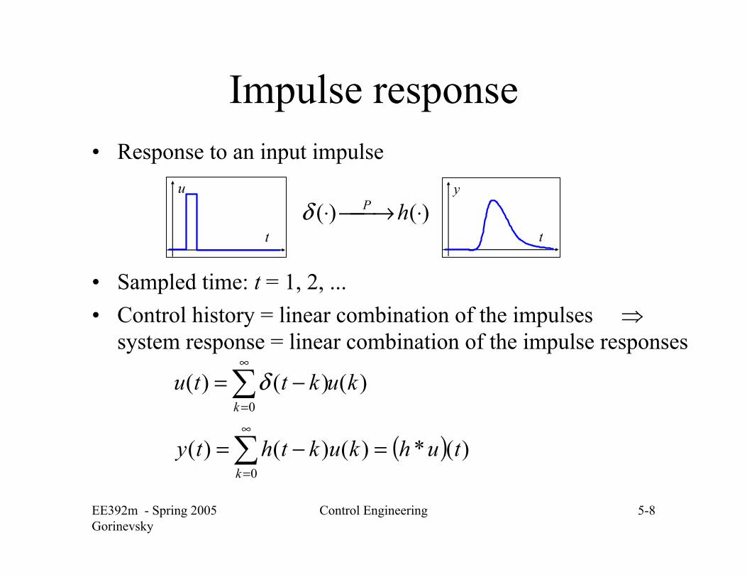
Impulse response • Response to an input impulse
• Sampled time: t = 1, 2, ...• Control history = linear combination of the impulses ⇒
system response = linear combination of the impulse responses
( ) )(*)()()(
)()()(
0
0
tuhkukthty
kukttu
k
k
=−=
−=
∑
∑∞
=
∞
=
δ
)()( ⋅⎯→⎯⋅ hPδu
t
y
t
EE392m - Spring 2005Gorinevsky
Control Engineering 5-9
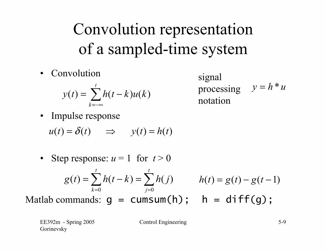
Convolution representation of a sampled-time system
• Convolution
• Impulse response
• Step response: u = 1 for t > 0
∑−∞=
−=t
k
kukthty )()()(
)()()()( thtyttu =⇒= δ
)1()()( −−= tgtgth
uhy *=signal processing notation
∑∑==
=−=t
j
t
k
jhkthtg00
)()()(
Matlab commands: g = cumsum(h); h = diff(g);
EE392m - Spring 2005Gorinevsky
Control Engineering 5-10
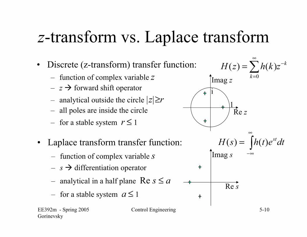
z-transform vs. Laplace transform• Discrete (z-transform) transfer function:
– function of complex variable z– z forward shift operator– analytical outside the circle |z|≥r– all poles are inside the circle– for a stable system r ≤ 1
k
k
zkhzH −∞
=∑=
0
)()(
• Laplace transform transfer function: – function of complex variable s– s differentiation operator
– analytical in a half plane Re s ≤ a– for a stable system a ≤ 1
∫∞
∞−
= dtethsH st)()(
Re s
Imag s
Re z
Imag z
1
i
EE392m - Spring 2005Gorinevsky
Control Engineering 5-11
Sampled time vs. continuous time
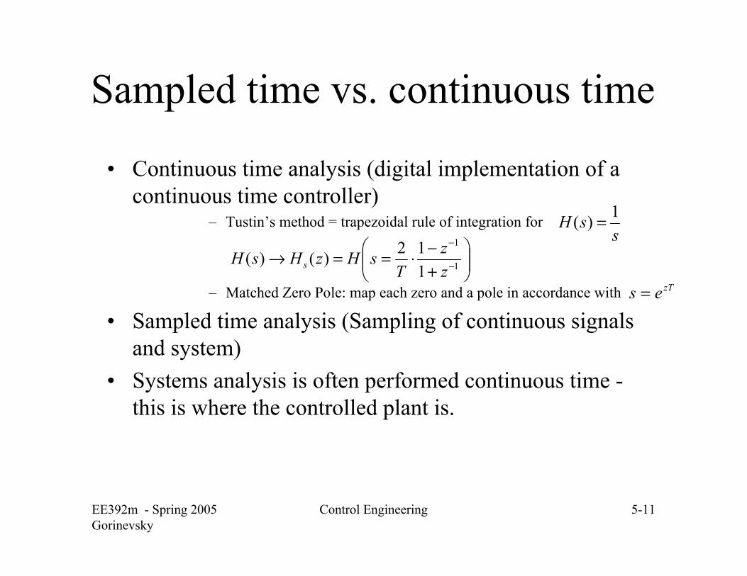
• Continuous time analysis (digital implementation of a continuous time controller)
– Tustin’s method = trapezoidal rule of integration for
– Matched Zero Pole: map each zero and a pole in accordance with
• Sampled time analysis (Sampling of continuous signals and system)
• Systems analysis is often performed continuous time -this is where the controlled plant is.
⎟⎟⎠
⎞⎜⎜⎝
⎛+−⋅==→ −
−
1
1
112)()(
zz
TsHzHsH s
ssH 1)( =
zTes =
EE392m - Spring 2005Gorinevsky
Control Engineering 5-12
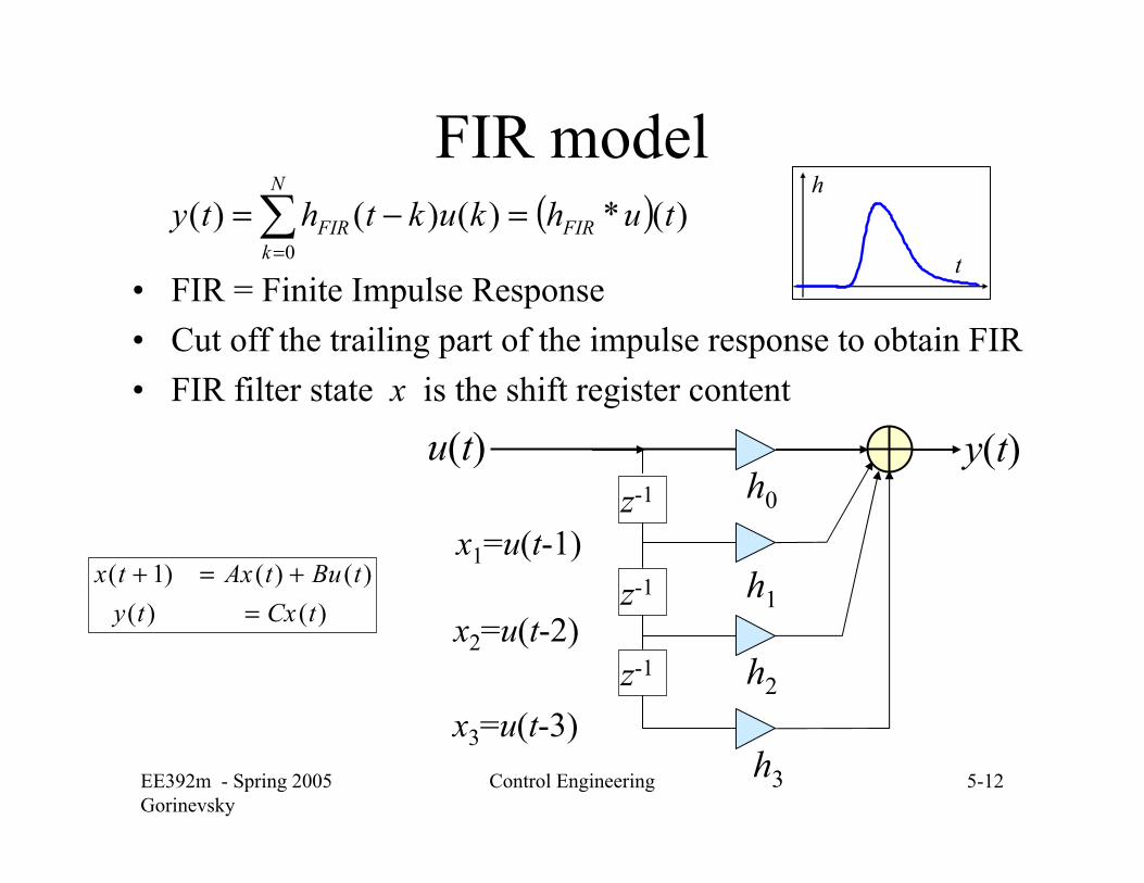
FIR model
• FIR = Finite Impulse Response • Cut off the trailing part of the impulse response to obtain FIR• FIR filter state x is the shift register content
h0
h1
h2
h3
u(t)
x1=u(t-1)
y(t)
x2=u(t-2)
x3=u(t-3)
z-1
z-1
z-1
( ) )(*)()()(0
tuhkukthty FIR
N
kFIR =−=∑
=
)()()()()1(
tCxtytButAxtx
=+=+
h
t
EE392m - Spring 2005Gorinevsky
Control Engineering 5-13
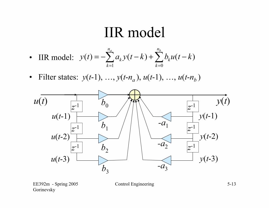
IIR model • IIR model:
• Filter states: y(t-1), …, y(t-na ), u(t-1), …, u(t-nb )
∑∑==
−+−−=ba n
kk
n
kk ktubktyaty
01
)()()(
u(t) b0
b1
b2
u(t-1)
u(t-2)
u(t-3)
z-1
z-1
z-1
-a1
-a2
y(t-1)
y(t-2)
y(t-3)
z-1
z-1
z-1
y(t)
b3-a3
EE392m - Spring 2005Gorinevsky
Control Engineering 5-14
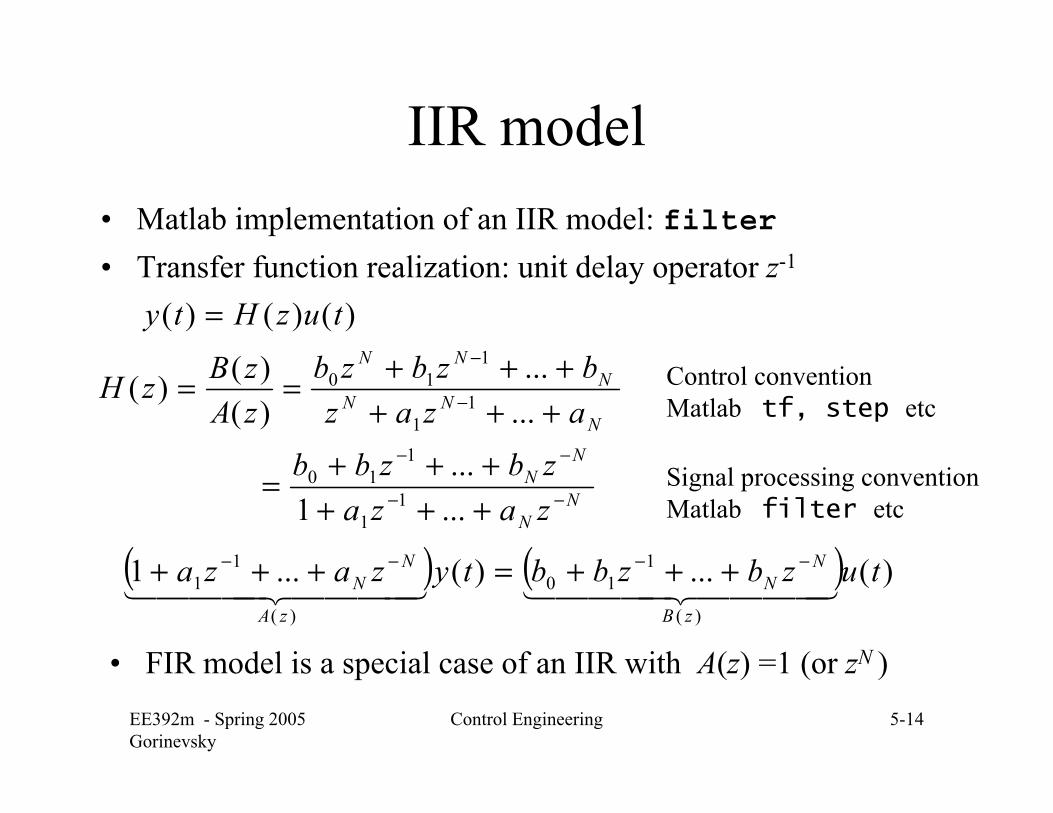
IIR model • Matlab implementation of an IIR model: filter• Transfer function realization: unit delay operator z-1
)()()( tuzHty =
• FIR model is a special case of an IIR with A(z) =1 (or zN )
( ) ( ) )(...)(...1)(
110
)(
11 tuzbzbbtyzaza
zB
NN
zA
NN 4444 34444 214444 34444 21
−−−− +++=+++
NN
NN
NNN
NNN
zazazbzbb
azazbzbzb
zAzBzH
−−
−−
−
−
++++++=
++++++==
...1...
......
)()()(
11
110
11
110
Signal processing conventionMatlab filter etc
Control conventionMatlab tf, step etc
EE392m - Spring 2005Gorinevsky
Control Engineering 5-15
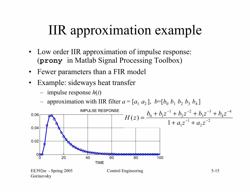
IIR approximation example• Low order IIR approximation of impulse response:
(prony in Matlab Signal Processing Toolbox) • Fewer parameters than a FIR model • Example: sideways heat transfer
– impulse response h(t)– approximation with IIR filter a = [a1 a2 ], b=[b0 b1 b2 b3 b4 ]
0 20 40 60 80 1000
0.02
0.04
0.06
TIME
IMPULSE RESPONSE
22
11
44
33
22
110
1)( −−
−−−−
++++++=
zazazbzbzbzbbzH
EE392m - Spring 2005Gorinevsky
Control Engineering 5-16
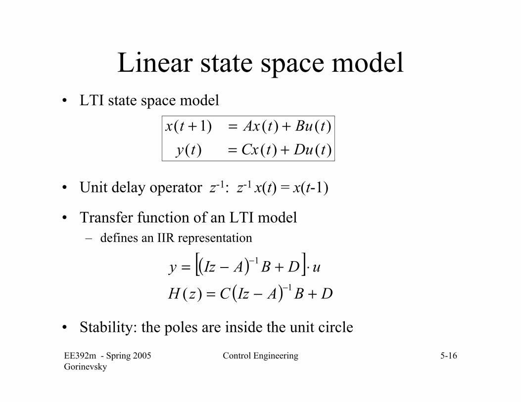
Linear state space model • LTI state space model
• Unit delay operator z-1: z-1 x(t) = x(t-1)
• Transfer function of an LTI model– defines an IIR representation
• Stability: the poles are inside the unit circle
( )[ ]( ) DBAIzCzH
uDBAIzy
+−=
⋅+−=−
−
1
1
)(
)()()()()()1(
tDutCxtytButAxtx
+=+=+
EE392m - Spring 2005Gorinevsky
Control Engineering 5-17
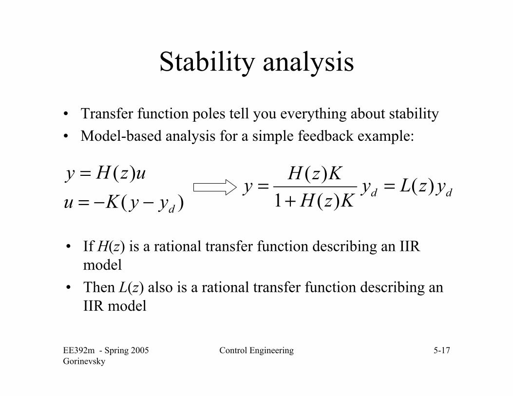
Stability analysis
• Transfer function poles tell you everything about stability• Model-based analysis for a simple feedback example:
)()(
dyyKuuzHy−−=
=dd yzLy
KzHKzHy )()(1
)( =+
=
• If H(z) is a rational transfer function describing an IIR model
• Then L(z) also is a rational transfer function describing an IIR model
EE392m - Spring 2005Gorinevsky
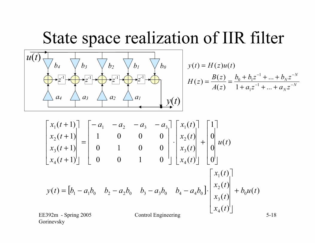
Control Engineering 5-18
[ ] )(
)()()()(
)(
)(
0001
)()()()(
010000100001
)1()1()1()1(
0
4
3
2
1
044033022011
4
3
2
13321
4
3
2
1
tub
txtxtxtx
babbabbabbabty
tu
txtxtxtxaaaa
txtxtxtx
+
⎥⎥⎥⎥
⎦
⎤
⎢⎢⎢⎢
⎣
⎡
⋅−−−−=
⎥⎥⎥⎥
⎦
⎤
⎢⎢⎢⎢
⎣
⎡
+
⎥⎥⎥⎥
⎦
⎤
⎢⎢⎢⎢
⎣
⎡
⋅
⎥⎥⎥⎥
⎦
⎤
⎢⎢⎢⎢
⎣
⎡ −−−−
=
⎥⎥⎥⎥
⎦
⎤
⎢⎢⎢⎢
⎣
⎡
++++
State space realization of IIR filter
y(t)
u(t)
a2a3a4 a1
b2b3b4 b1 b0
z-1 z-1 z-1 z-1
NN
NN
zazazbzbb
zAzBzH
tuzHty
−−
−−
++++++==
=
...1...
)()()(
)()()(
11
110
EE392m - Spring 2005Gorinevsky
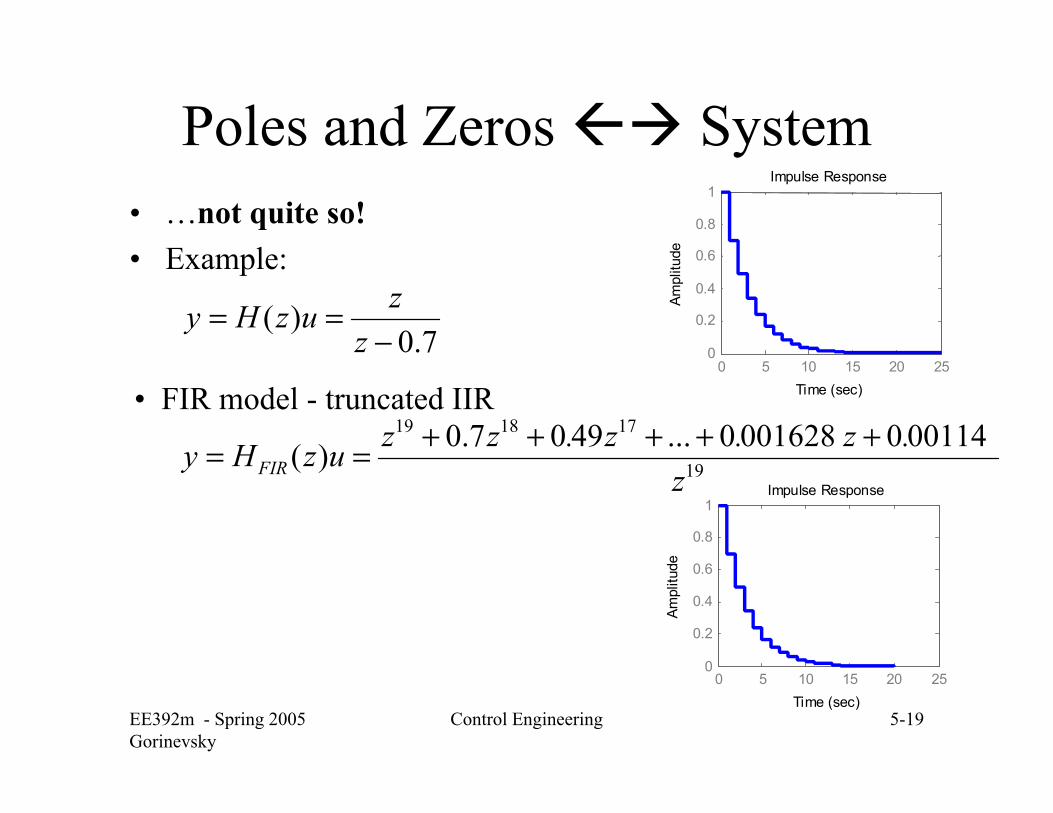
Control Engineering 5-19
Poles and Zeros System • …not quite so!• Example:
7.0)(
−==
zzuzHy
19
171819 0011400016280...4907.0)(z
. z.z.zzuzHy FIR+++++==
Impulse Response
Time (sec)
Ampl
itude
0 5 10 15 20 250
0.2
0.4
0.6
0.8
1
Impulse Response
Time (sec)
Ampl
itude
0 5 10 15 20 250
0.2
0.4
0.6
0.8
1
• FIR model - truncated IIR
EE392m - Spring 2005Gorinevsky
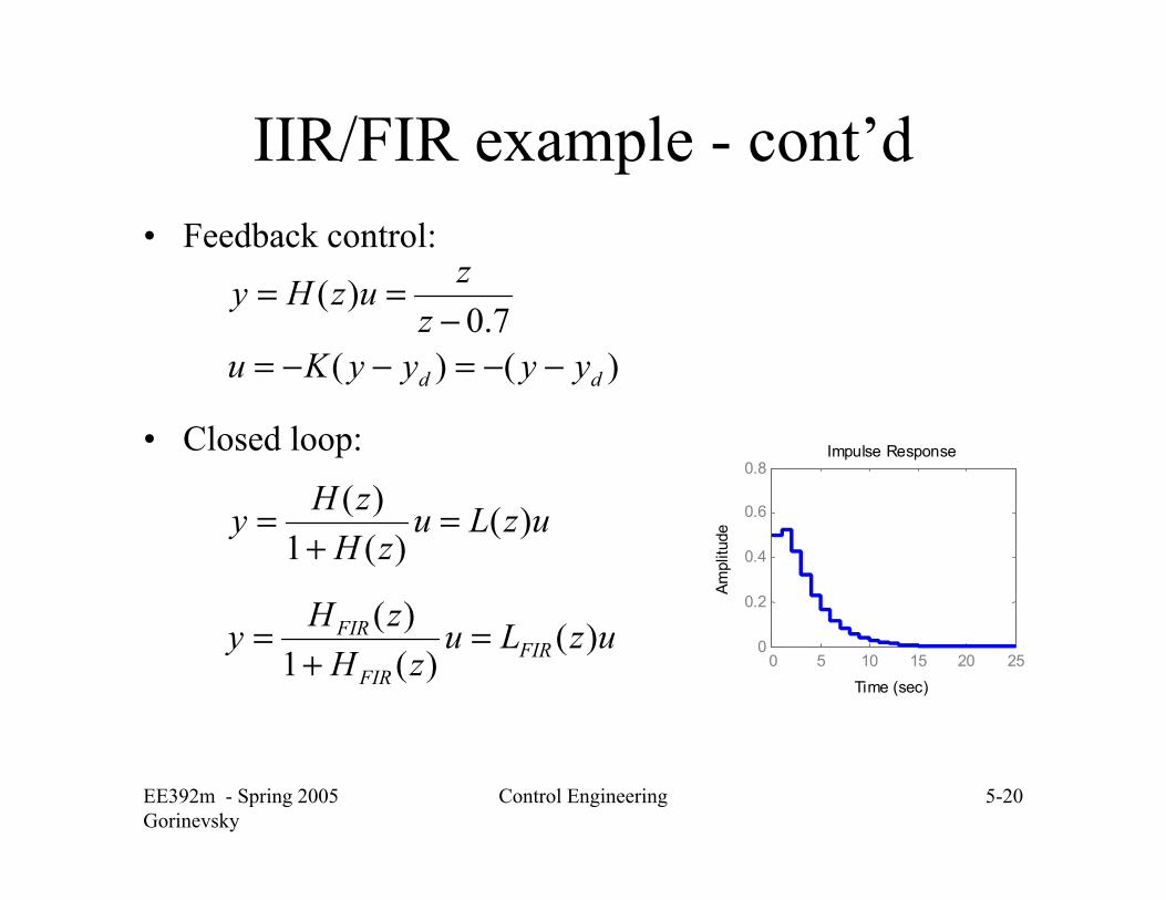
Control Engineering 5-20
IIR/FIR example - cont’d • Feedback control:
• Closed loop:
)()(7.0
)(
dd yyyyKuz
zuzHy
−−=−−=−
==
Impulse Response
Time (sec)
Ampl
itude
0 5 10 15 20 250
0.2
0.4
0.6
0.8
uzLuzH
zHy )()(1
)( =+
=
uzLuzH
zHy FIRFIR
FIR )()(1
)( =+
=
EE392m - Spring 2005Gorinevsky
Control Engineering 5-21
-0.8 -0.6 -0.4 -0.2 0 0.2 0.4 0.6 0.8-0.8
-0.6
-0.4
-0.2
0
0.2
0.4
0.6
0.8
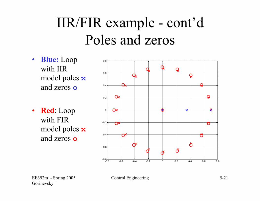
IIR/FIR example - cont’dPoles and zeros
• Blue: Loop with IIR model poles xand zeros o
• Red: Loop with FIR model poles xand zeros o
EE392m - Spring 2005Gorinevsky
Control Engineering 5-22
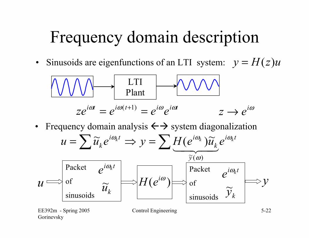
Frequency domain description• Sinusoids are eigenfunctions of an LTI system:
LTIPlant
tiititi eeeze ωωωω == + )1(
• Frequency domain analysis system diagonalization
uzHy )(=
∑∑ =⇒= ti
y
kiti
kkkk eueHyeuu ω
ω
ωω
43421)(~
~)(~
k
ti
ue k
~ω
uPacket
of
sinusoids
Packet
of
sinusoids
)( ωieH y
ωiez →
k
ti
ye k
~ω
EE392m - Spring 2005Gorinevsky
Control Engineering 5-23
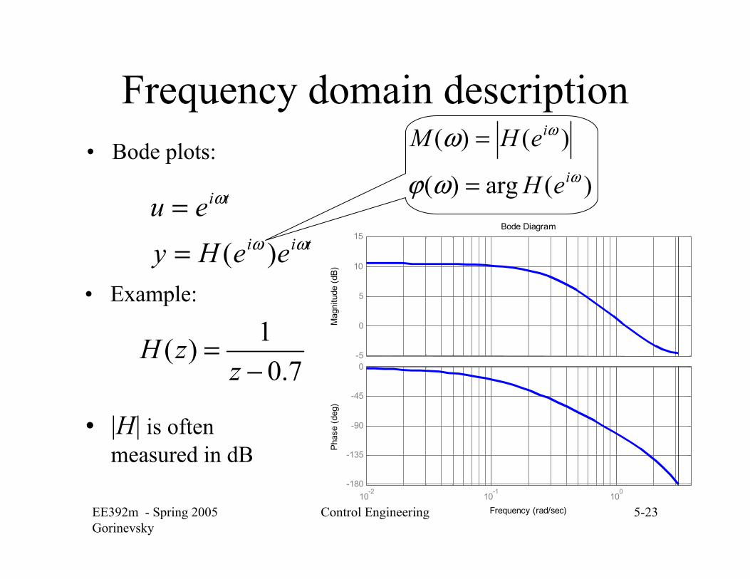
Frequency domain description• Bode plots:
tii
ti
eeHyeu
ωω
ω
)(==
• Example:
)(arg)(
)()(ω
ω
ωϕ
ωi
i
eH
eHM
=
=
7.01)(
−=
zzH
Bode Diagram
Frequency (rad/sec)
Phas
e (d
eg)
Mag
nitu
de (d
B)
-5
0
5
10
15
10-2
10-1
100
-180
-135
-90
-45
0
• |H| is often measured in dB
EE392m - Spring 2005Gorinevsky
Control Engineering 5-24
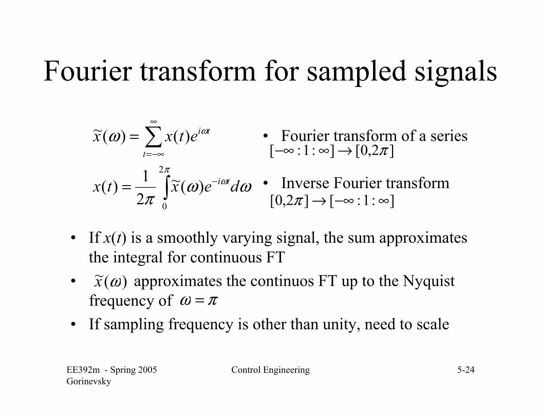
Fourier transform for sampled signals
• Fourier transform of a series
• Inverse Fourier transform∫
∑
−
∞
−∞=
=
=
πω
ω
ωωπ
ω
2
0
)(~21)(
)()(~
dextx
etxx
ti
t
ti
]2,0[]:1:[ π→∞−∞
]:1:[]2,0[ ∞−∞→π
• If x(t) is a smoothly varying signal, the sum approximates the integral for continuous FT
• approximates the continuos FT up to the Nyquist frequency of
• If sampling frequency is other than unity, need to scale
)(~ ωxπω =
EE392m - Spring 2005Gorinevsky
Control Engineering 5-25
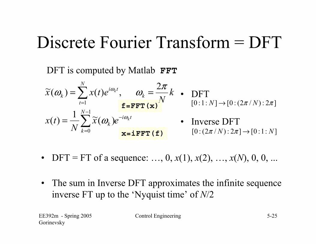
Discrete Fourier Transform = DFT
• DFT
• Inverse DFTtiN
kk
k
N
t
tik
k
k
exN
tx
kN
etxx
ω
ω
ω
πωω
−−
=
=
∑
∑
=
==
1
0
1
)(~1)(
2,)()(~]2:)/2(:0[]:1:0[ ππ NN →
]:1:0[]2:)/2(:0[ NN →ππ
• DFT = FT of a sequence: …, 0, x(1), x(2), …, x(N), 0, 0, ...
• The sum in Inverse DFT approximates the infinite sequence inverse FT up to the ‘Nyquist time’ of N/2
DFT is computed by Matlab FFT
x=iFFT(f)
f=FFT(x)
EE392m - Spring 2005Gorinevsky
Control Engineering 5-26
Sampled-time LTI models - recap
• Linear system can be described by impulse response• Linear system can be described by frequency response =
Fourier transform of the impulse response • FIR, IIR, State-space models can be used to obtain close
approximations of sampled-time linear system • A pattern of poles and zeros can be very different for a
small change in an input-output model. • Impulse response, step response, and frequency response
do not change much for small model changes
EE392m - Spring 2005Gorinevsky
Control Engineering 5-27
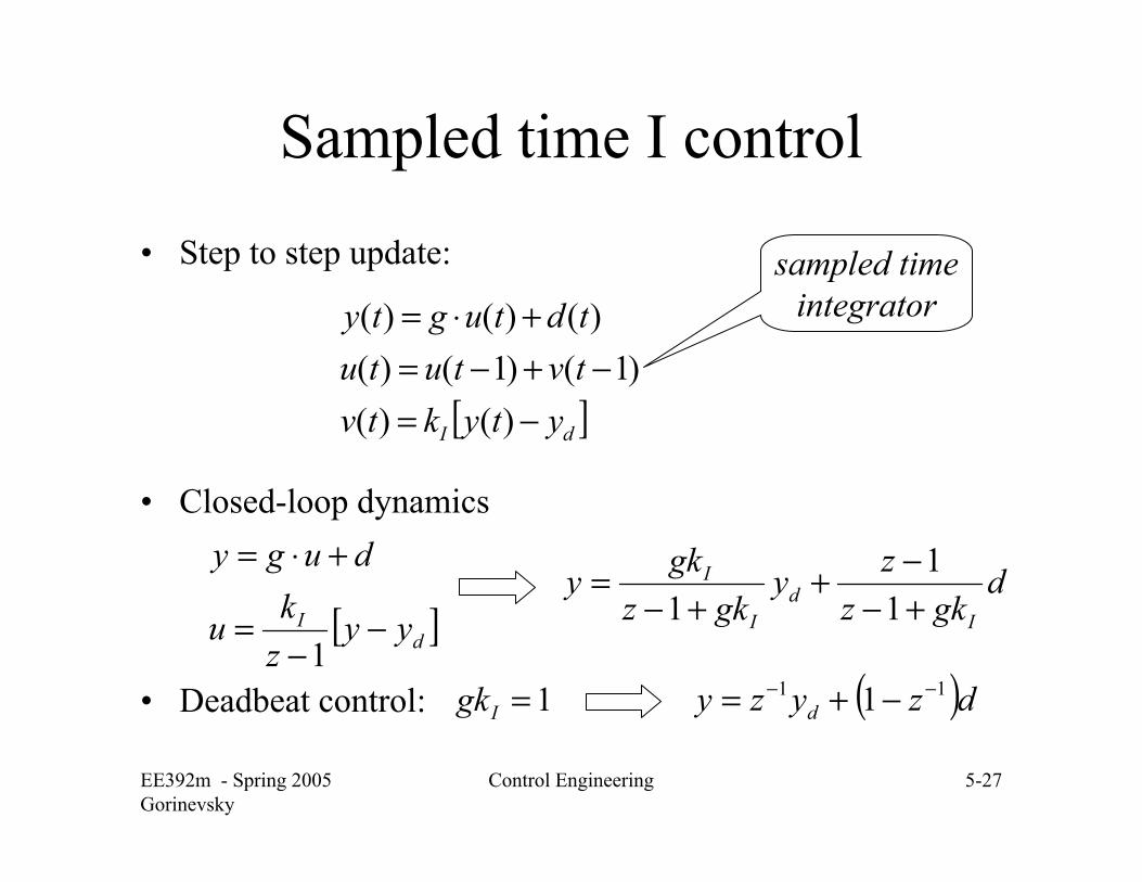
Sampled time I control
• Step to step update:
• Closed-loop dynamics
• Deadbeat control:
[ ]dI ytyktvtvtututdtugty
−=−+−=
+⋅=
)()()1()1()(
)()()(
[ ]dI yy
zku
dugy
−−
=
+⋅=
1
dgkz
zygkz
gkyI
dI
I
+−−+
+−=
11
1
sampled timeintegrator
1=Igk ( )dzyzy d11 1 −− −+=
EE392m - Spring 2005Gorinevsky
Control Engineering 5-28
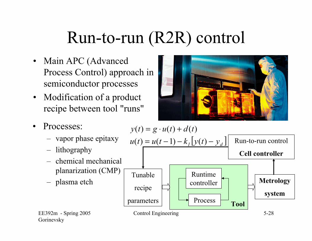
Run-to-run (R2R) control• Main APC (Advanced
Process Control) approach in semiconductor processes
• Modification of a product recipe between tool "runs"
Tool
Run-to-run control
Cell controller
Process
Runtime controller Metrology
system
Tunable
recipe
parameters
• Processes:– vapor phase epitaxy– lithography – chemical mechanical
planarization (CMP)– plasma etch
[ ]dI ytyktututdtugty
−−−=+⋅=
)()1()()()()(
EE392m - Spring 2005Gorinevsky
Control Engineering 5-29
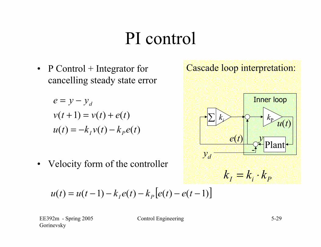
Cascade loop interpretation:
PI control• P Control + Integrator for
cancelling steady state error
• Velocity form of the controller
)()()()()()1(
tektvktutetvtv
yye
PI
d
−−=+=+
−= Inner loop
Plant
kP
e(t)u(t)
ki∑
y-yd
PiI kkk ⋅=[ ])1()()()1()( −−−−−= tetektektutu PI
EE392m - Spring 2005Gorinevsky
Control Engineering 5-30
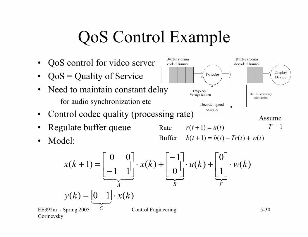
QoS Control Example• QoS control for video server• QoS = Quality of Service • Need to maintain constant delay
– for audio synchronization etc
• Control codec quality (processing rate)• Regulate buffer queue• Model: )()()()1(
)()1(twtTrtbtb
tutr+−=+
=+RateBuffer
AssumeT = 1
{ {
[ ] )(10)(
)(10
)(01
)(1100
)1(
kxky
kwkukxkx
C
FBA
⋅=
⋅⎥⎦
⎤⎢⎣
⎡+⋅⎥⎦
⎤⎢⎣
⎡−+⋅⎥⎦
⎤⎢⎣
⎡−
=+
321
43421
EE392m - Spring 2005Gorinevsky
Control Engineering 5-31
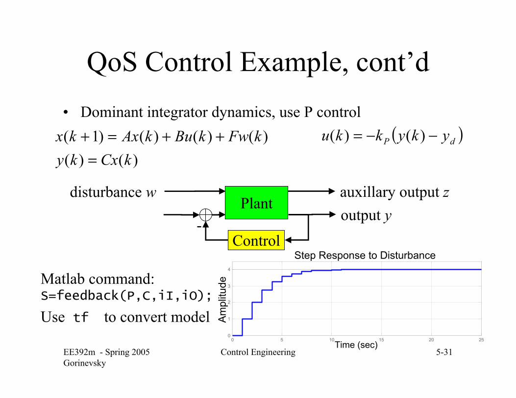
QoS Control Example, cont’d• Dominant integrator dynamics, use P control
)()()()()()1(
kCxkykFwkBukAxkx
=++=+ ( )dP ykykku −−= )()(
output yPlant
Control
disturbance w
-
auxillary output z
Matlab command: S=feedback(P,C,iI,iO);
Use tf to convert model25.0=Pk
0 5 10 15 20 250
1
2
3
4
Step Response to Disturbance
Time (sec)
Am
plitu
de
EE392m - Spring 2005Gorinevsky
Control Engineering 5-32
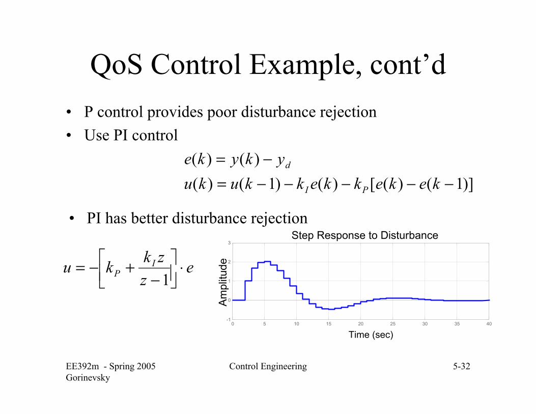
QoS Control Example, cont’d• P control provides poor disturbance rejection• Use PI control
)]1()([)()1()()()(
−−−−−=−=
kekekkekkukuykyke
PI
d
ez
zkku IP ⋅⎥⎦
⎤⎢⎣⎡
−+−=
1
• PI has better disturbance rejection
1.025.0
==
I
P
kk
0 5 10 15 20 25 30 35 40-1
0
1
2
3Step Response to Disturbance
Time (sec)
Am
plitu
de
EE392m - Spring 2005Gorinevsky
Control Engineering 5-33
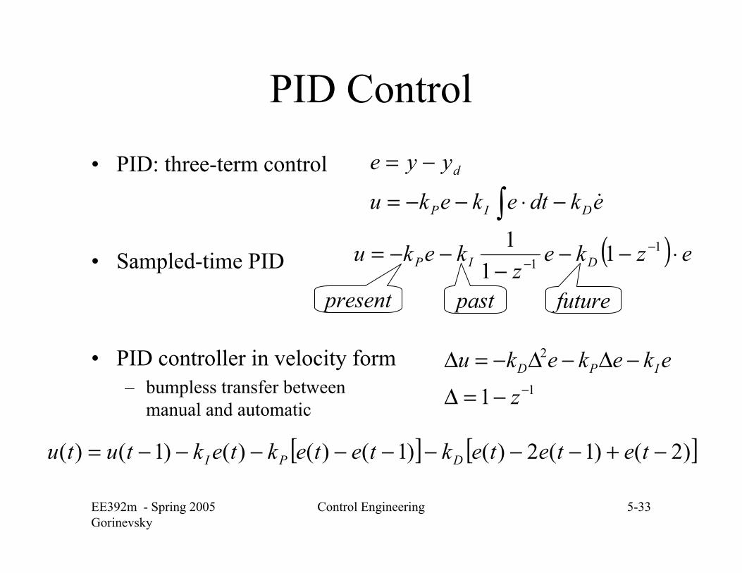
PID Control
• PID: three-term control
• Sampled-time PID
• PID controller in velocity form– bumpless transfer between
manual and automatic
ekdtekeku
yye
DIP
d
&−⋅−−=
−=
∫( ) ezke
zkeku DIP ⋅−−
−−−= −
−1
1 11
1
futurepresent past
[ ] [ ])2()1(2)()1()()()1()( −+−−−−−−−−= tetetektetektektutu DPI
1
2
1 −−=∆
−∆−∆−=∆
zekekeku IPD
EE392m - Spring 2005Gorinevsky
Control Engineering 5-34
PID Controller Tuning
• Tune continuous-time PID controller, e.g. by Ziegler-Nichols rule, and set up the sampled time PID to approximate the continuous-time PID
• Cascaded loop design (continuous time structure) – Design P – Cascade I, retune P– Add D, retune PI
• Optimize the performance parameters by repeated simulation runs – search through the {P, I, D} space
• Loopshaping – Lectures 7-8 • Advanced control design – formal specs, other courses
EE392m - Spring 2005Gorinevsky
Control Engineering 5-35
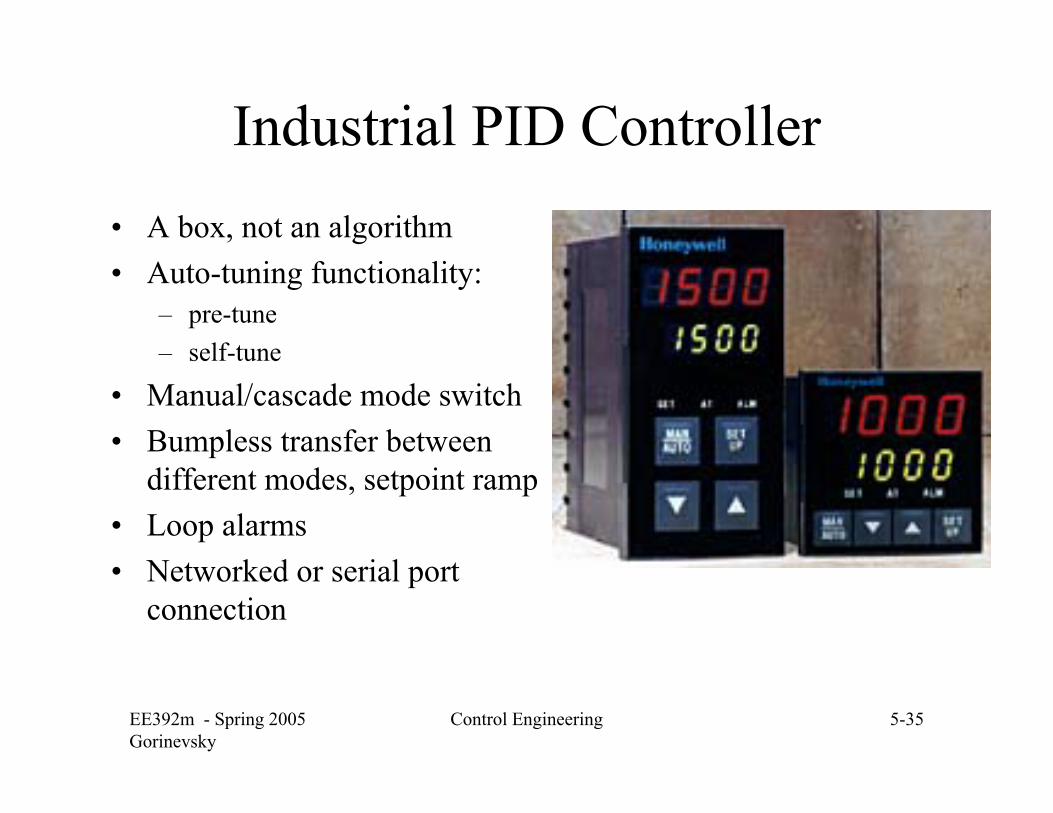
Industrial PID Controller• A box, not an algorithm• Auto-tuning functionality:
– pre-tune– self-tune
• Manual/cascade mode switch• Bumpless transfer between
different modes, setpoint ramp• Loop alarms • Networked or serial port
connection
EE392m - Spring 2005Gorinevsky
Control Engineering 5-36
Plant Type
• Constant gain - I control• Integrator - P control • First order system - PI control • Double integrator or second order system - PD control• Generic response with delay - PID control