Lecture 2: Smoothed Particle Hydrodynamics (SPH)

Formulation

Professor G.R. Liu SMA Fellow, Director, ACES Centre

Department of Mechanical Engineering, National University of Singapore (Office: EA-5-05; Tel: 6516-6481; E-mail: mpeliugr@nus.edu.sg)

http://www.nus.edu.sg/ACES/

Collaborator: Dr. Li Zirui

Introduction to SPH

Basic concepts of computational hydrodynamics

• Grid based methodsEulerian approach (FDM)Lagrangian approach (FEM)Meshfree methods can use both approaches

• Particle based methodsSmoothed Particle HydrodynamicsDissipative Particle DynamicsBrownian Dynamics

• A typical numerical simulation of a CFD problem involves the following factors.

Governing equations,

Proper boundary conditions and/or initial conditions,

Domain discretization,

Formulation technique,

Solving the resultant algebraic equations or ordinary differential equations (ODE).

Introduction to SPH

Eulerian vs Lagrangian descriptions Lagrangian methods Eulerian methods

Grid Attached on the moving material Fixed in the space

Track Movement of any point on materials Mass, momentum, and energy flux across grid nodes and mesh cell boundary

Time history Easy to obtain time-history data at a point attached on materials

Difficult to obtain time-history data at a point attached on materials

Moving boundary and interface

Easy to track Difficult to track

Irregular geometry Easy to model Difficult to model with good accuracy

Large deformation Difficult to handle Easy to handle

Introduction to SPH: descriptions

Meshfree particle methods (MPMs)Methods References

Molecular dynamics (MD) Alder and Wainright ,1957; Rahman, 1964; Stillinger and Rahman, 1974; etc.

Monte Carlo (MC) Metropolis and Ulam, 1949; Binder, 1988, 1992; etc.

Direct simulation Monte Carlo (DSMC) Bird, 1994; Pan et al., 1999, 2000, 2002; etc.

Dissipative particle dynamics (DPD) Hoogerbrugge and Koelman, 1992; Español, 1998; etc.

Lattice gas Cellular Automata (CA) Wolfram, 1983; Kandanoff et al. 1989; etc.

Lattice Bolztmann equation (LBE) Chen and Doolen, 1998; Qian et al., 2000; etc.

Particle-in-Cell (PIC) Harlow, 1963; 1964; etc.

Marker-and-Cell (MAC) Harlow, 1964; etc.

Fluid-in-Cell (FLIC) Gentry et al., 1966; etc.

Moving Particle Semi-implicit (MPS) Koshizuka et al., 1998; etc.

Discrete element method (DEM) Cundall, 1987; Owen, 1996; etc.

Vortex methods Chorin, 1973; Leonard, 1980; etc.

Smoothed particle hydrodynamics (SPH) Lucy, 1977; Gingold and Monaghan, 1977; etc.

Introduction to SPH

Grid based methodsthe Eulerian description is a spatial description, e.g. FDMthe Lagrangian description is a material description, e.g.FEM

DDt t

αα

∂ ∂= +∂ ∂

vx

SPH: derivatives

N.S equations for inviscid, no heat transfer flows

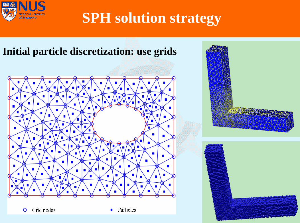
Initial particle discretization: use grids

SPH solution strategy

To approximate the values of functions, derivatives at a particle using the information at all the neighboring particles

1

( ) ( )N

i ii

u uφ=

=∑x x

SPH: Particle approximation

SPH Formulation

Basic concepts (particle and explicit)

1. Discretization using a set of arbitrarily distributed particles.2. Integral function approximation: kernel approximation3. Particle approximation of field functions.

Summation to replace integrationField function and its derivatives

4. PDEs are represented directly in particle approximation.5. No connectivity is defined between particles: large

deformation.6. The ODE's are solved using explicit integration algorithm:

explicit.

Integral representation of a function

• Starting form

• Replace by a smoothing function

• W is the so-called smoothing kernel function, or smoothing function, or smoothing kernel, or kernel function or kernel

∫Ω

′′−′= xxxxx dff )()()( δ

1( )

0δ

′=⎧′− = ⎨ ′≠⎩

x xx x

x x

)( xx ′−δ ),( hW xx ′−

( ) ( ) ( , )f f W h dΩ

′ ′ ′≈ −∫x x x x x

( ) ( ) ( , )f f W h dΩ

′ ′ ′< >= −∫x x x x x

SPH Formulation: function approximation

Basic properties of smoothing function

• Normalization condition (unity condition)

• Delta function property

• Compact condition

k is a constant related to the smoothing function for point at x, and defines the

effective (non-zero) area of the smoothing function.

∫Ω

=′′− 1),( xxx dhW

)(),(lim0

xxxx ′−=′−→

δhWh

( , ) 0W h′− =x x hκ′∀ − >x x

SPH Formulation: function approximation

Derivative of a function

( ) [ ( )] ( , )f f W h dΩ

′ ′ ′< ∇ >= ∇ −∫x x x x x

[ ( )] ( , )[ ( ) ( , )] ( ) ( , )

f W hf W h f W h

′ ′∇ − =′ ′ ′ ′∇ − − ⋅∇ −

x x xx x x x x x

( )

[ ( ) ( , )] ( ) ( , )

f

f W h d f W h dΩ Ω

< ∇ ⋅ >=

′ ′ ′ ′ ′ ′∇ − − ∇ −∫ ∫x

x x x x x x x x

0, S

( ) ( ) ( , ) ( ) ( , )onS

f f W h dS f W h d= Ω

′ ′ ′ ′ ′< ∇⋅ >= − ⋅ − ⋅∇ −∫ ∫x x x x n x x x x

( ) ( ) ( , )f f W h dΩ

′ ′ ′< ∇ ⋅ >= − ⋅∇ −∫x x x x x

SPH Formulation: function approximation

Boundary effects

( ) ( ) ( , ) ( ) ( , )S

f f W h dS f W h dΩ

′ ′ ′ ′ ′< ∇ ⋅ >= − ⋅ − ⋅∇ −∫ ∫x x x x n x x x x0≠

Special treatment required

( ) ( ) ( , )f f W h dΩ

′ ′ ′< ∇ ⋅ >= − ⋅∇ −∫x x x x x

0=

SPH Formulation: function approximation

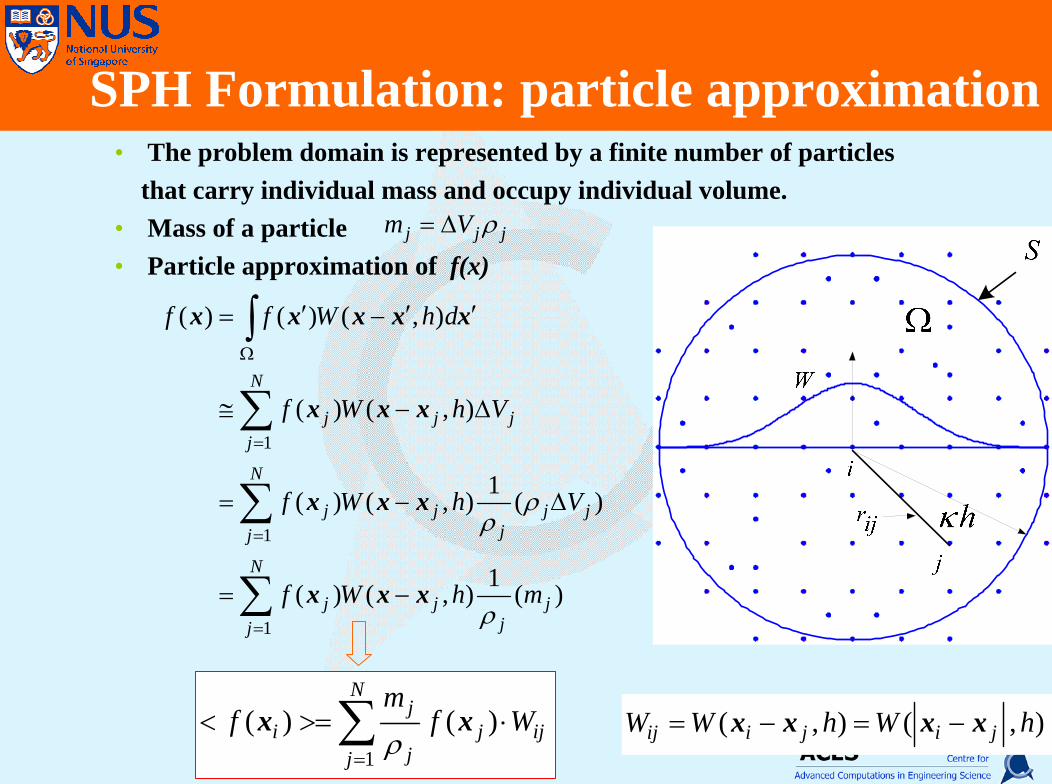
• The problem domain is represented by a finite number of particles that carry individual mass and occupy individual volume.

• Mass of a particle• Particle approximation of f(x)

j j jm V ρ= ∆

1

1

1

( ) ( ) ( , )

( ) ( , )

1( ) ( , ) ( )

1( ) ( , ) ( )

N

j j jj

N

j j j jjj

N

j j jjj

f f W h d

f W h V

f W h V

f W h m

ρρ

ρ

Ω

=

=

=

′ ′ ′= −

≅ − ∆

= − ∆

= −

∫

∑

∑

∑

x x x x x

x x x

x x x

x x x

1

( ) ( )N

ji j ij

jj

mf f W

ρ=

< >= ⋅∑x x ( , ) ( , )ij i j i jW W h W h= − = −x x x x

SPH Formulation: particle approximation

1

( ) ( ) ( , )N

jj j

jj

mf f W h

ρ=

< ∇ ⋅ >= − ⋅∇ −∑x x x x

i j ij ij iji ij

ij ij ij ij

W WW

r r r r− ∂ ∂

∇ = =∂ ∂

x x x

∑=

=N

jijji Wm

1

ρ

SPH Formulation: particle approximation

Function

1

( ) ( )N

ji j i ij

jj

mf f W

ρ=

< ∇⋅ >= − ⋅∇∑x x

1

( ) ( )N

ji j ij

jj

mf f W

ρ=

< >= ⋅∑x x

Derivative of a function

• The support domain for a field point at x is the domain where the information for all the points inside this domain is used to determine the information at the point at x .

• The influence domain is defined as a domain where a node exerts its influences.

• When the concept of support domain is used, the consideration is based on a field point; When the concept of influence domain is used, the consideration is based only on the nodes.

• If a node i is within the support domain of a point x, then node i exert an influence on point x, and thus point x is within the influence domain of node i.

Particle selection: support & influence domains

Particle selection: support & influence domains

Support domain

Influence domain

• The SPH method employs particles to represent material and form the computational frame. There is no need for predefined connectivity between these particles. All one needs is the initial particle distribution.

• The SPH approximation consists of kernel approximation and particle approximation. The kernel approximation of a function and its derivative are carried out in the continuum domain, and the particle approximations of a function and its derivative are carried out using discretized particles in the support domain.

• Each particle in the SPH method is associated with a support domain and influence domain. For most practical applications, the support domain of a particle can be equal to its influence domain.

SPH Formulation: concluding remarks

1) Liu G.R. and Liu M.B., Smoothed Particle Hydrodynamics: a meshfree particle method, World Scientific, 1st printing (2003), 3rd printing (2007)

2) Liu GR, Meshfree methods: moving beyond the finite element method. 1st Edition (2002), 2nd Edition (2009), CRC Press.

3) Monaghan J.J., Smoothed Particle Hydrodynamics, Annual Review of Astronomy and Astrophysics, 30:543-574, (1992)

4) Lucy L.B., Numerical approach to testing the fission hypothesis, Astronomical Journal, 82:1013-1024, (1977)

5) Benz W., Smoothed Particle Hydrodynamics: a review, NATO workshop, Les; Arcs, France, (1989)

SPH: references

AcknowledgementsDr. M.B. Liu Etc.