Embed Size (px)
Citation preview

DISC Systems and Control Theory of Nonlinear Systems 1
Lecture 2:Controllability of nonlinear systems
Nonlinear Dynamical Control Systems, Chapter 3
See www.math.rug.nl/˜arjan (under teaching) for info on course
schedule and homework sets.
Take-Home Exam I on homepage on March 16.

DISC Systems and Control Theory of Nonlinear Systems 2
Recall: Kinematic model of the unicycle
x1 = u1 cosx3
x2 = u1 sinx3
x3 = u2
written as a system with two input vector fields and zero drift
vector field
x =
cosx3
sin x3
0
u1 +
0
0
1
u2
The Lie bracket of the two input vector fields is given as
−
0 0 − sinx3
0 0 cosx3
0 0 0
0
0
1
=
sinx3
− cosx3
0

DISC Systems and Control Theory of Nonlinear Systems 3
which is a vector field that is independent from the two input
vector fields.
Claim: This new independent direction guarantees controllability
of the unicycle system.
Interpretation of the Lie bracket:
Proposition 1 Let X, Y be two vector fields such that
[X, Y ] = 0
Then the solution flows of the vector fields are commuting.
In fact, we may find local coordinates x1, . . . , xn such that
X =∂
∂x1, Y =
∂
∂x2
Thus, the Lie bracket [X, Y ] characterizes the amount of
non-commutativity of the vector fields X, Y .
DISC Systems and Control Theory of Nonlinear Systems 4
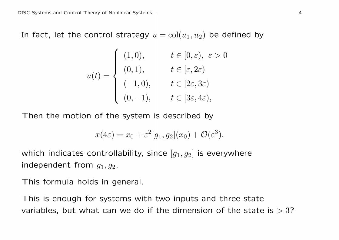
In fact, let the control strategy u = col(u1, u2) be defined by
u(t) =
(1, 0), t ∈ [0, ε), ε > 0
(0, 1), t ∈ [ε, 2ε)
(−1, 0), t ∈ [2ε, 3ε)
(0,−1), t ∈ [3ε, 4ε),
Then the motion of the system is described by
x(4ε) = x0 + ε2[g1, g2](x0) + O(ε3).
which indicates controllability, since [g1, g2] is everywhere
independent from g1, g2.
This formula holds in general.
This is enough for systems with two inputs and three state
variables, but what can we do if the dimension of the state is > 3?
DISC Systems and Control Theory of Nonlinear Systems 5
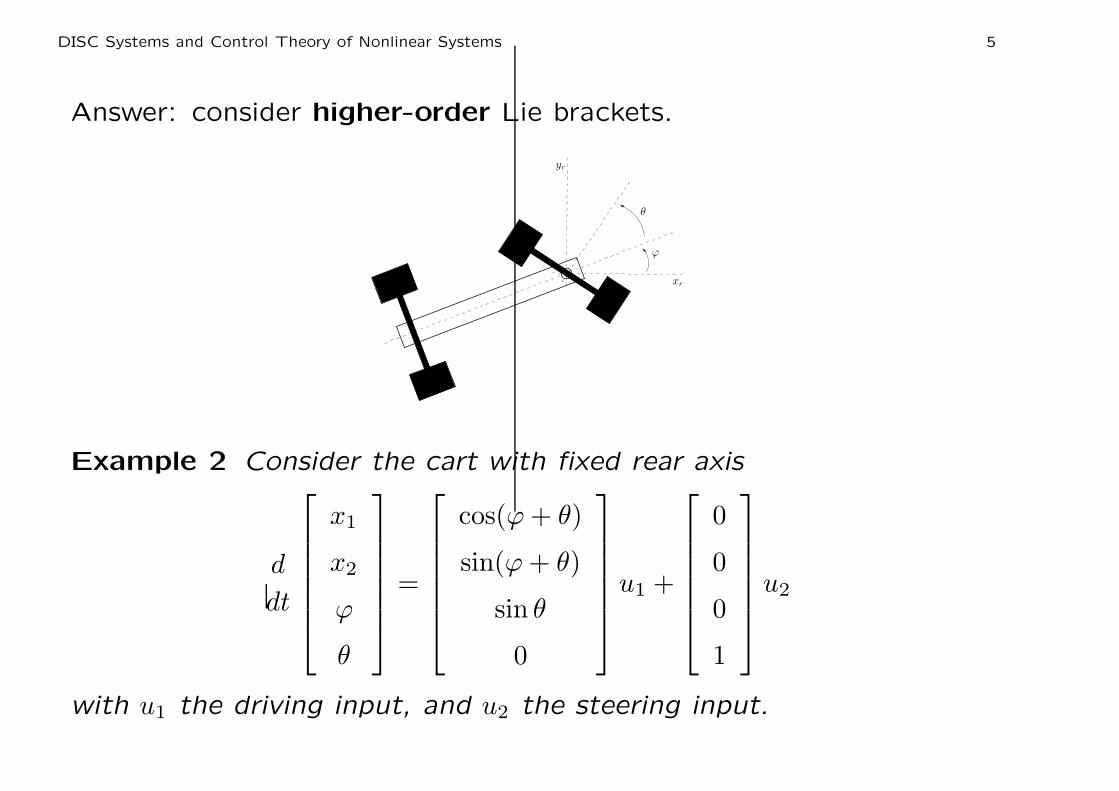
Answer: consider higher-order Lie brackets.
I
M
yr
θ
ϕ
xr
Example 2 Consider the cart with fixed rear axis
d
dt
x1
x2
ϕ
θ
=
cos(ϕ + θ)
sin(ϕ + θ)
sin θ
0
u1 +
0
0
0
1
u2
with u1 the driving input, and u2 the steering input.
DISC Systems and Control Theory of Nonlinear Systems 6
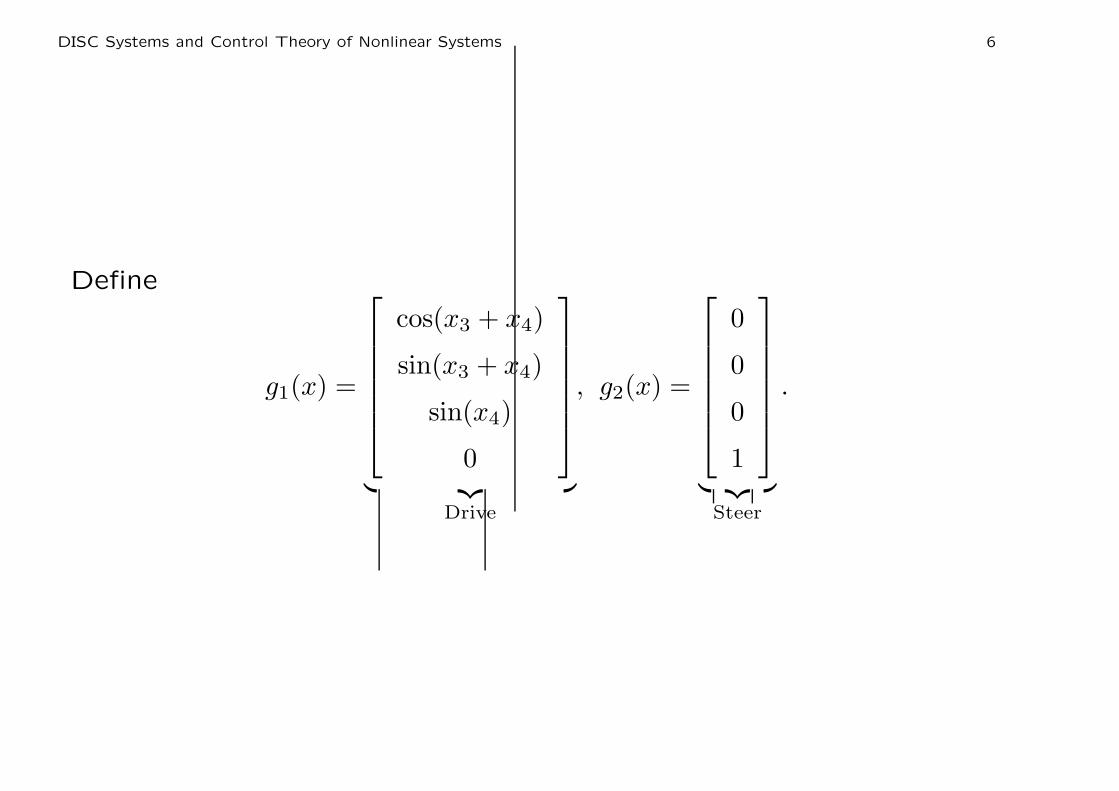
Define
g1(x) =
cos(x3 + x4)
sin(x3 + x4)
sin(x4)
0
︸ ︷︷ ︸
Drive
, g2(x) =
0
0
0
1
︸ ︷︷ ︸
Steer
.

DISC Systems and Control Theory of Nonlinear Systems 7
Compute
[Steer, Drive] =∂g1
∂xg2 −
∂g2
∂xg1
=
0 0 − sin(x3 + x4) − sin(x3 + x4)
0 0 cos(x3 + x4) cos(x3 + x4)
0 0 0 cos(x4)
0 0 0 0
0
0
0
1
− 0
=
− sin(x3 + x4)
cos(x3 + x4)
cos(x4)
0
=: Wriggle.
DISC Systems and Control Theory of Nonlinear Systems 8
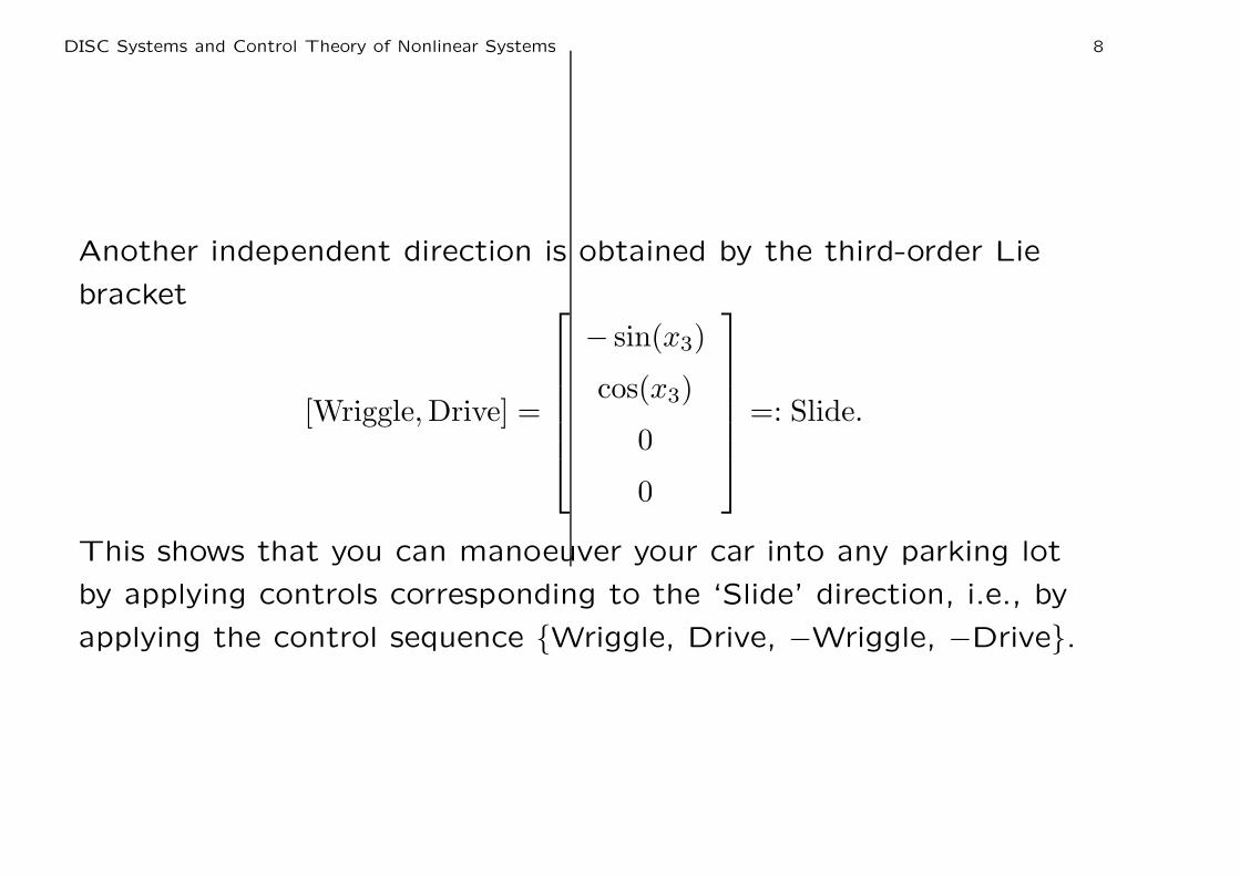
Another independent direction is obtained by the third-order Lie
bracket
[Wriggle, Drive] =
− sin(x3)
cos(x3)
0
0
=: Slide.
This shows that you can manoeuver your car into any parking lot
by applying controls corresponding to the ‘Slide’ direction, i.e., by
applying the control sequence {Wriggle, Drive, −Wriggle, −Drive}.

DISC Systems and Control Theory of Nonlinear Systems 9
What to do with the drift vector field ?
The system
x = f(x) + g(x)u
can be considered as a special case of
x = g1(x)u1 + g2(x)u2,
with u1 = 1. This means that care has to be taken with respect to
brackets involving f :
[f, g], [g, [f, g]], [f, [f, g]], . . .

DISC Systems and Control Theory of Nonlinear Systems 10
Example 3 Consider the system on R2
x1 = x22
x2 = u.
Compute the Lie brackets of the vector fields
f(x) =
x2
2
0
, g(x) =
0
1
,
yielding
[f, g](x) =
−2x2
0
, [[f, g], g](x) =
2
0
.
Clearly, we have obtained two independent directions. However,
since x22 ≥ 0, the x1-coordinate is always non-decreasing. Hence,
the system is not really controllable.
DISC Systems and Control Theory of Nonlinear Systems 11
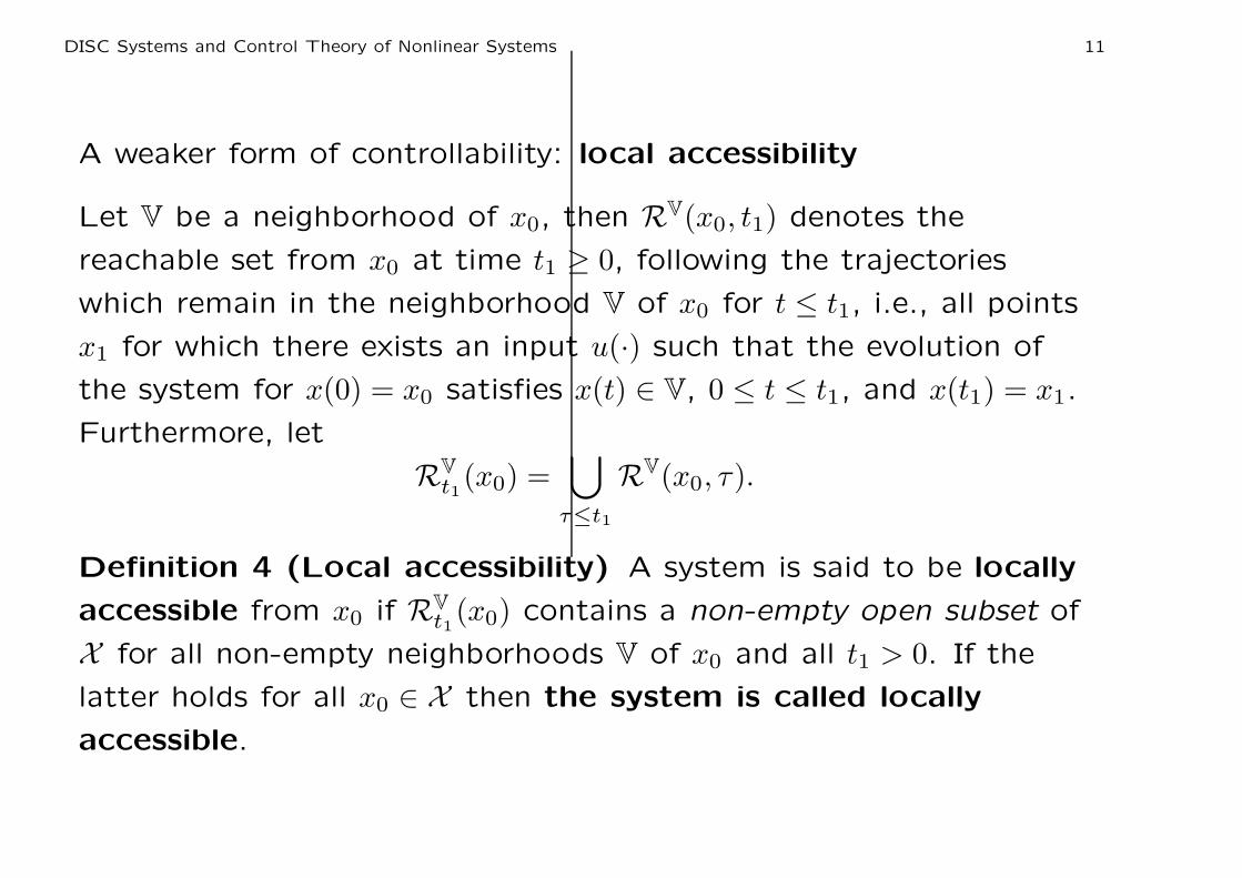
A weaker form of controllability: local accessibility
Let V be a neighborhood of x0, then RV(x0, t1) denotes the
reachable set from x0 at time t1 ≥ 0, following the trajectories
which remain in the neighborhood V of x0 for t ≤ t1, i.e., all points
x1 for which there exists an input u(·) such that the evolution of
the system for x(0) = x0 satisfies x(t) ∈ V, 0 ≤ t ≤ t1, and x(t1) = x1.
Furthermore, let
RV
t1(x0) =
⋃
τ≤t1
RV(x0, τ).
Definition 4 (Local accessibility) A system is said to be locally
accessible from x0 if RVt1
(x0) contains a non-empty open subset of
X for all non-empty neighborhoods V of x0 and all t1 > 0. If the
latter holds for all x0 ∈ X then the system is called locally
accessible.

DISC Systems and Control Theory of Nonlinear Systems 12
Definition 5 (Accessibility algebra) Consider the system
x = f(x) + g1(x)u1 + · · · + gm(x)um
The accessibility algebra C are the linear combinations of
repeated Lie brackets of the form
[Xk, [Xk−1, [· · · , [X2, X1] · · · ]]], k = 1, 2, . . . ,
where Xi, is a vector field in the set {f, g1, . . . , gm}.
This linear space is a Lie algebra under the Lie bracket.
Definition 6 The accessibility distribution C is the distribution
generated by the accessibility algebra C:
C(x) = span{X(x) | X vector field in C}, x ∈ X
DISC Systems and Control Theory of Nonlinear Systems 13
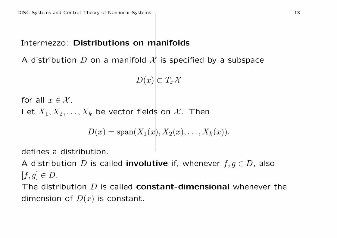
Intermezzo: Distributions on manifolds
A distribution D on a manifold X is specified by a subspace
D(x) ⊂ TxX
for all x ∈ X .
Let X1, X2, . . . , Xk be vector fields on X . Then
D(x) = span(X1(x), X2(x), . . . , Xk(x)).
defines a distribution.
A distribution D is called involutive if, whenever f, g ∈ D, also
[f, g] ∈ D.
The distribution D is called constant-dimensional whenever the
dimension of D(x) is constant.

DISC Systems and Control Theory of Nonlinear Systems 14
Example 7 Let X = R3 and D = span(f1, f2), where
f1(x) =
2x2
1
0
, f2(x) =
1
0
x2
.
Since f1 and f2 are linearly independent, we have that
dim(D(x)) = 2, for all x. Furthermore, we have
[f1, f2](x) =∂f2
∂x(x)f1(x) −
∂f1
∂x(x)f2(x) =
1
0
0
.

DISC Systems and Control Theory of Nonlinear Systems 15
[f1, f2] ∈ D if and only if rank(f1(x), f2(x), [f1, f2](x)) = 2, for all x.
However,
rank(f1(x), f2(x), [f1, f2](x)) = rank
2x2 1 0
1 0 0
0 x2 1
= 3,
for all x. Hence, D is not involutive.
DISC Systems and Control Theory of Nonlinear Systems 16
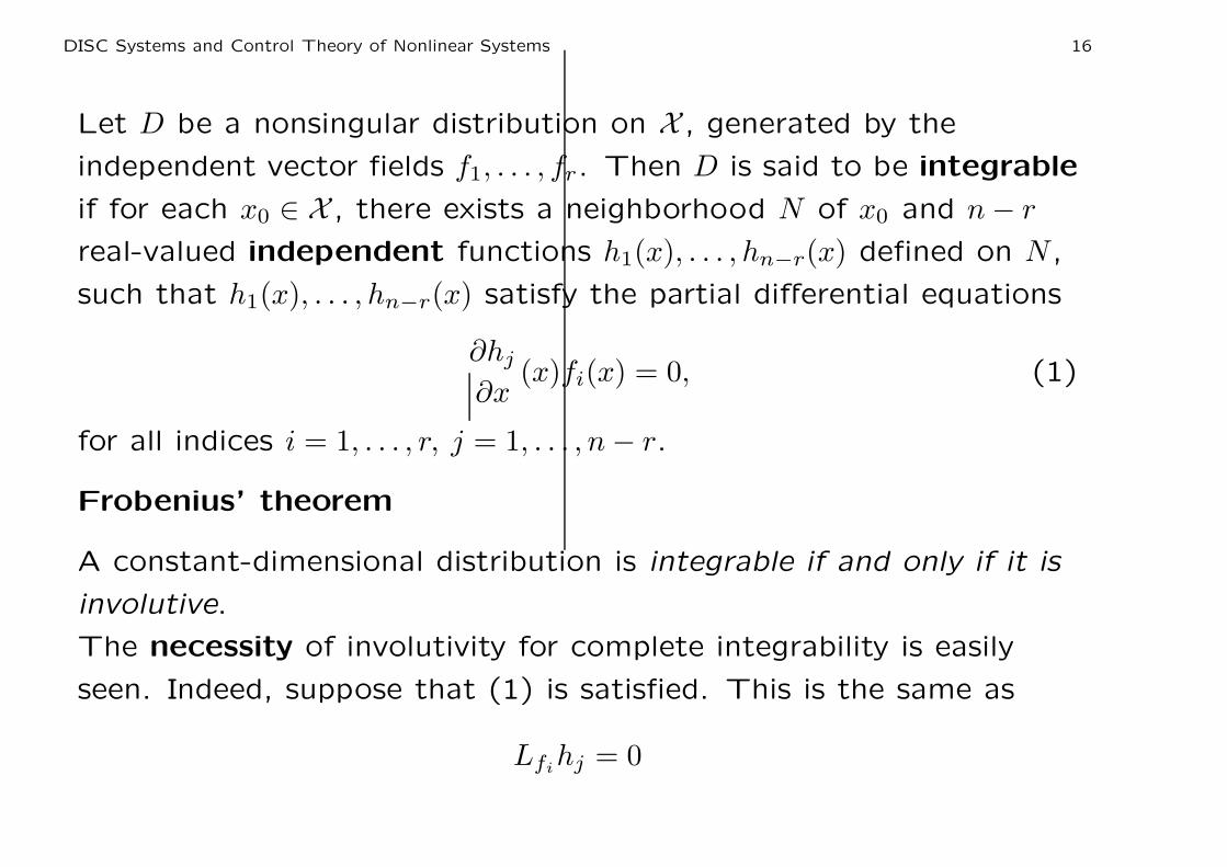
Let D be a nonsingular distribution on X , generated by the
independent vector fields f1, . . . , fr. Then D is said to be integrable
if for each x0 ∈ X , there exists a neighborhood N of x0 and n − r
real-valued independent functions h1(x), . . . , hn−r(x) defined on N ,
such that h1(x), . . . , hn−r(x) satisfy the partial differential equations
∂hj
∂x(x)fi(x) = 0, (1)
for all indices i = 1, . . . , r, j = 1, . . . , n − r.
Frobenius’ theorem
A constant-dimensional distribution is integrable if and only if it is
involutive.
The necessity of involutivity for complete integrability is easily
seen. Indeed, suppose that (1) is satisfied. This is the same as
Lfihj = 0

DISC Systems and Control Theory of Nonlinear Systems 17
It follows that
L[fi,fk]hj = LfiLfk
hj − LfkLfi
hj = 0
Since the functions h1(x), . . . , hn−r(x) are independent, this implies
that the Lie brackets [fi, fk] are (pointwise) linear combinations of
the vector fields f1, . . . , fr, and are thus contained in the
distribution D.
A geometric description of Frobenius’ theorem is as follows. Let
the independent functions h1(x), . . . , hn−r(x) satisfy (1). Then their
level sets, i.e., all sets of the form
{x | h1(x) = c1, . . . , hn−r(x) = cn−r}
for arbitrary constants c1, . . . , cn−r, are well-defined r-dimensional
submanifolds of X , to which all the vector fields f1, . . . , fr are
tangent, and, as a consequence, also all their Lie brackets are
tangent.
DISC Systems and Control Theory of Nonlinear Systems 18
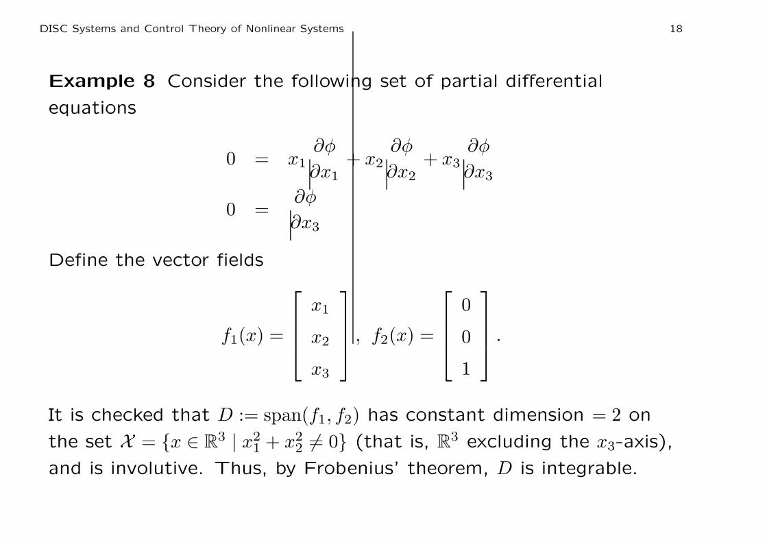
Example 8 Consider the following set of partial differential
equations
0 = x1∂φ
∂x1+ x2
∂φ
∂x2+ x3
∂φ
∂x3
0 =∂φ
∂x3
Define the vector fields
f1(x) =
x1
x2
x3
, f2(x) =
0
0
1
.
It is checked that D := span(f1, f2) has constant dimension = 2 on
the set X = {x ∈ R3 | x2
1 + x22 6= 0} (that is, R
3 excluding the x3-axis),
and is involutive. Thus, by Frobenius’ theorem, D is integrable.

DISC Systems and Control Theory of Nonlinear Systems 19
Consequently, for each x0 ∈ X , there exists a neighborhood N of x0
and a real-valued function φ(x) with dφ(x) 6= 0 that satisfies the
given set of partial differential equations. In fact, φ(x) = lnx1 − lnx2
is a (global) solution.
Note that the solution is not unique. In particular, φ(x) = tan−1 x2
x1
is
also a global solution.

DISC Systems and Control Theory of Nonlinear Systems 20
By construction, the accessibility distribution C is involutive.
Theorem 9 (Local accessibility) A sufficient condition for the
system to be locally accessible from x ∈ X is
dimC(x) = n (2)
If this holds for all x ∈ X then the system is locally accessible.
Conversely, if the system is locally accessible then (2) holds for all
x in an open and dense subset of X .
We call (2) the accessibility rank condition at x.

DISC Systems and Control Theory of Nonlinear Systems 21
Key idea of the proof
Consider the system
x = f(x) + g1(x)u1 + . . . gm(x)um
and its generated system vector fields
F = {X | ∃u1, . . . , um such that X(x) = f(x) + g1(x)u1 + . . . gm(x)um}
Then for every k ≤ n there exists a submanifold Nk around x0 of
dimension k given as
Nk = {x | x = Xtk
k ◦ Xtk−1
k−1 ◦ · · · ◦ Xt11 (x0), 0 ≤ σi < ti < τi}
with Xi ∈ F. Indeed, suppose for a certain k < n we cannot
construct Nk+1. This means that all system vector fields X ∈ F are
tangent to Nk, and hence all vector fields f, g1, . . . , gm. This also
means that all Lie brackets of these vector fields are tangent to
Nk, and thus dim C(x) ≤ k, which is a contradiction.
DISC Systems and Control Theory of Nonlinear Systems 22
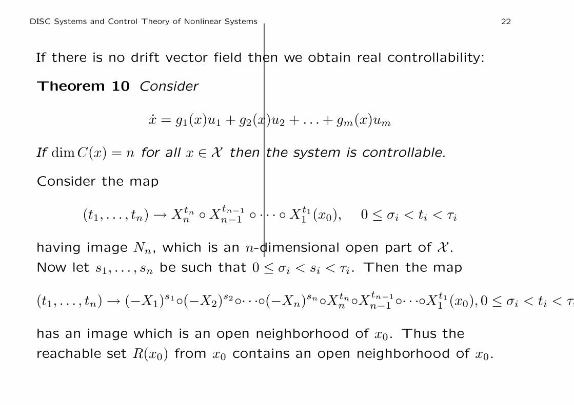
If there is no drift vector field then we obtain real controllability:
Theorem 10 Consider
x = g1(x)u1 + g2(x)u2 + . . . + gm(x)um
If dimC(x) = n for all x ∈ X then the system is controllable.
Consider the map
(t1, . . . , tn) → Xtn
n ◦ Xtn−1
n−1 ◦ · · · ◦ Xt11 (x0), 0 ≤ σi < ti < τi
having image Nn, which is an n-dimensional open part of X .
Now let s1, . . . , sn be such that 0 ≤ σi < si < τi. Then the map
(t1, . . . , tn) → (−X1)s1◦(−X2)
s2◦· · ·◦(−Xn)sn◦Xtn
n ◦Xtn−1
n−1 ◦· · ·◦Xt11 (x0), 0 ≤ σi < ti < τi
has an image which is an open neighborhood of x0. Thus the
reachable set R(x0) from x0 contains an open neighborhood of x0.
DISC Systems and Control Theory of Nonlinear Systems 23
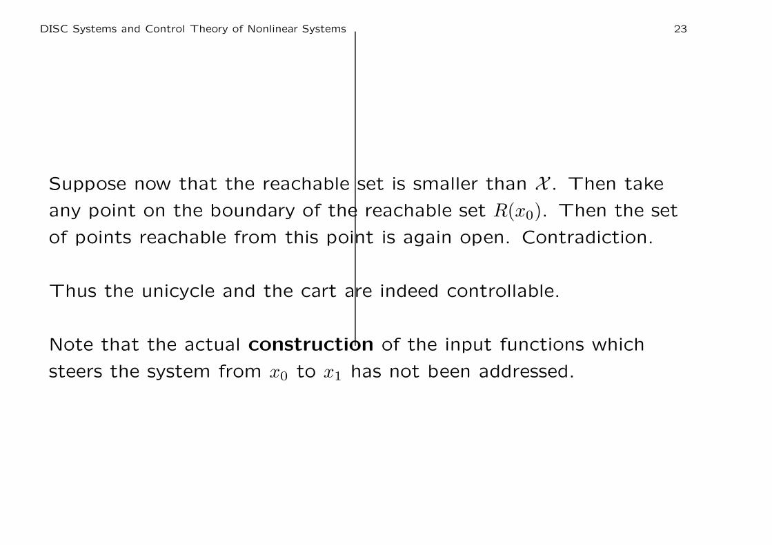
Suppose now that the reachable set is smaller than X . Then take
any point on the boundary of the reachable set R(x0). Then the set
of points reachable from this point is again open. Contradiction.
Thus the unicycle and the cart are indeed controllable.
Note that the actual construction of the input functions which
steers the system from x0 to x1 has not been addressed.

DISC Systems and Control Theory of Nonlinear Systems 24
Sometimes local accessibility is heavily depending on the flow of
the drift vector field; consider for example the system
x1 = 1
x2 = u
This system is locally accessible, but of course very far from
controllability. In order to improve the situation we look at a
stronger form of accessibility: local strong accessibility
A system is locally strongly accessible from x0 if for any
neighborhood V of x0 the set RV(x0, t1) contains a non-empty set
for any t1 > 0 sufficiently small. If the latter holds for all x ∈ X then
the system is called locally strongly accessible.
(The example given above is not locally strongly accessible.)

DISC Systems and Control Theory of Nonlinear Systems 25
Define C0 as the smallest algebra which contains g1, . . . , gm and
satisfies [f, w] ∈ C0 for all w ∈ C0. Define the corresponding
involutive distribution
C0(x) := span{X(x) | X vector field in C0}.
We refer to C0 and C0 as the strong accessibility algebra and the
strong accessibility distribution, respectively.

DISC Systems and Control Theory of Nonlinear Systems 26
Notice that the strong accessibility algebra C0 does not contain the
drift vector field f).
Theorem 11 (Strong accessibility) A sufficient condition for the
system to be locally strongly accessible from x is
dimC0(x) = n
Furthermore, the system is locally strongly accessible if this holds
for all x. Conversely, if the system is locally strongly accessible
then it holds for all x in an open and dense subset of X .
The system given before:
x1 = x22
x2 = u.
is not only locally accessible, but also locally strongly accessible,
since g(x) and [[f, g], g](x) are everywhere independent.
DISC Systems and Control Theory of Nonlinear Systems 27
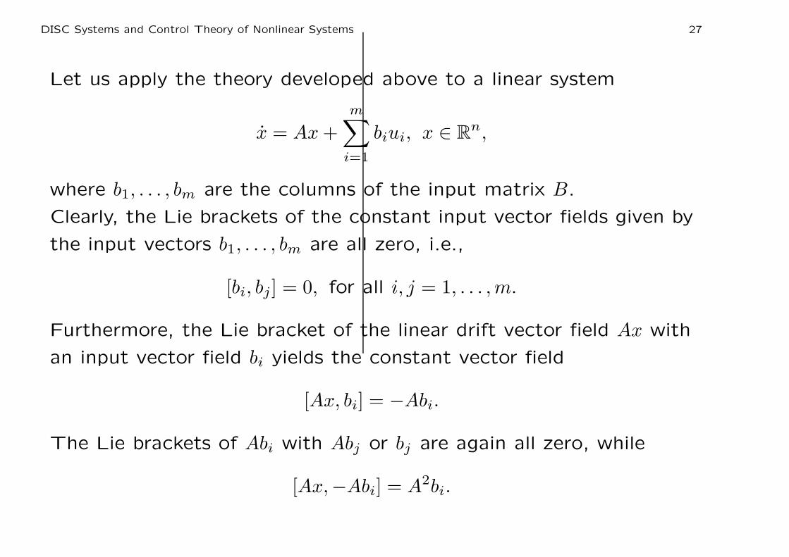
Let us apply the theory developed above to a linear system
x = Ax +
m∑
i=1
biui, x ∈ Rn,
where b1, . . . , bm are the columns of the input matrix B.
Clearly, the Lie brackets of the constant input vector fields given by
the input vectors b1, . . . , bm are all zero, i.e.,
[bi, bj ] = 0, for all i, j = 1, . . . , m.
Furthermore, the Lie bracket of the linear drift vector field Ax with
an input vector field bi yields the constant vector field
[Ax, bi] = −Abi.
The Lie brackets of Abi with Abj or bj are again all zero, while
[Ax,−Abi] = A2bi.

DISC Systems and Control Theory of Nonlinear Systems 28
Hence we conclude that C is spanned by all constant vector fields
bi, Abi, A2bi, . . . , i ∈ m, together with the linear drift vector field Ax,
i.e.,
C = {Ax, bi, Abi, A2bi . . . , An−1bi, i = 1, . . . , m}.
while
C0 = columns of (B, AB, A2B . . . , An−1B)
We see that for linear systems the rank condition for strong
accessibility coincides with the Kalman rank condition for
controllability. Hence, if we would not have known anything special
about linear systems, then at least a linear system which satisfies
the Kalman rank condition is locally strongly accessible.

DISC Systems and Control Theory of Nonlinear Systems 29
Example 12 (Actuated rotating rigid body)
Consider
ω1
ω2
ω3
=
A1ω2ω3
A2ω3ω1
A3ω1ω2
+
α1
0
0
u1 +
0
α2
0
u2
with α1 6= 0, α2 6= 0. Here the constants A1, A2, A3 are determined by
the moments of inertia a1, a2, a3. Compute
[g1, f ](ω) =
0
α1A2ω3
α1A3ω2
[g2, f ](ω) =
α2A1ω3
0
α2A3ω1
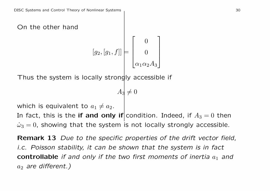
DISC Systems and Control Theory of Nonlinear Systems 30
On the other hand
[g2, [g1, f ]] =
0
0
α1α2A3
Thus the system is locally strongly accessible if
A3 6= 0
which is equivalent to a1 6= a2.
In fact, this is the if and only if condition. Indeed, if A3 = 0 then
ω3 = 0, showing that the system is not locally strongly accessible.
Remark 13 Due to the specific properties of the drift vector field,
i.c. Poisson stability, it can be shown that the system is in fact
controllable if and only if the two first moments of inertia a1 and
a2 are different.)


![Nonlinear Programming Models Fabio Schoen Introductionfor all x,y ∈ Ω,λ ∈ [0,1] Nonlinear Programming Models – p. 5 Convex Functions x y Nonlinear Programming Models – p](https://img.dokumen.tips/doc/110x75/60025c042470c9743d105bb3/nonlinear-programming-models-fabio-schoen-for-all-xy-a-a-01-nonlinear.jpg)


![Minotaur: A Mixed-Integer Nonlinear Optimization Toolkit^2 + x 1 x 2 Fig. 2 A directed acyclic graph representing the nonlinear function x 1(x 1 + x 2) + (x 1 + x 2)2. 74]. These solvers](https://img.dokumen.tips/doc/110x75/5fc79d5a038f585712232324/minotaur-a-mixed-integer-nonlinear-optimization-2-x-1-x-2-fig-2-a-directed.jpg)