Embed Size (px)
Citation preview

Dynamics of multiphoton processes innonlinear optics and x-ray
spectroscopy
Ji-Cai Liu
Department of Theoretical Chemistry
School of Biotechnology
Royal Institute of Technology
Stockholm, Sweden 2009
c© Ji-Cai Liu, 2009
ISBN 978-91-7415-480-1
ISSN 1654-2312
TRITA-BIO Report 2009:25
Printed by Universitetsservice US AB,
Stockholm, Sweden, 2009

Abstract
New generations of ultrashort and intense laser pulses as well as high power synchrotron
radiation sources and x-ray free electron lasers have promoted fast developments in nonlinear
optics and x-ray spectroscopy. The new experimental achievements and the appearance
of varieties of novel nonlinear phenomena call for further development of theories. The
objective of this thesis is to develop and apply the theories to explain existing experimental
data and to suggest new experiments.
The first part of the thesis is devoted to nonlinear propagation of optical pulses. It is shown
that the vibrational levels can be selectively populated by varying the duration, shape
and intensity of the pump pulse. We obtained a strict analytical solution for the resonant
two-photon interaction in a multilevel system beyond rotating wave approximation. Simu-
lations show that the polarization anisotropy of the two-photon excitation affects strongly
the anisotropy of photobleaching. The two-photon area theorem is reformulated with tak-
ing into account the dynamical Stark shift and the contribution from the permanent dipole
moments. In general the dynamical Stark shift does not allow complete population of the
excited state, but it can be compensated by detunings in atoms. A dynamical theory of
the sequential two-photon absorption of microsecond pulses is developed to explore the role
of transverse inhomogeneity of the light beam on optical limiting properties. The propaga-
tion of ultrashort laser pulses in nondipolar and dipolar media is investigated with special
attention to the generation of superfluorescence and supercontinuum and the formation of
attosecond pulses.
The second part of the thesis addresses the interaction of molecules with x-ray radiation.
We explore here the role of nuclear dynamics in resonant Auger scattering. Multimode
simulations of the Auger spectra of ethylene molecule explain the main spectral features of
the experimental spectra and show that the spectral profiles are formed mainly due to six
vibrational modes. We predict the Doppler splitting of the atomic peak in resonant Auger
scattering from SF6 molecule for circularly polarized x-rays. This effect is confirmed by
the recent experiment. A new scheme of x-ray pump-probe spectroscopy, namely, resonant
inelastic x-ray scattering accompanied by core-hole hopping induced by strong laser fields
is suggested. The laser-induced promotion of core holes opens the symmetry forbidden
scattering channels and gives rise to new spectral lines in the x-ray scattering spectrum. The
strength of the symmetry forbidden lines becomes strong when the time of Rabi flopping
is shorter than the lifetime of the core-excited state. We study the role of propagation of
femtosecond x-ray free-electron pulses on the Auger process. Simulations show that there
exists a strong competition between Auger decay and stimulated emission. The Auger yield
and Auger branching ratio are strongly suppressed in the course of pulse propagation.

Preface
The work presented in this thesis has been carried out during a period of about 2.5 years,
April 2007 - December 2009, at the Department of Theoretical Chemistry, School of Biotech-
nology, Royal Institute of Technology, Stockholm, Sweden.
List of papers included in the thesis
Paper I J.-C. Liu, V. C. Felicissimo, F. F. Guimaraes, C.-K. Wang, and F. Gel’mukhanov,
Coherent control of population and pulse propagation beyond the rotating wave approxima-
tion, J. Phys. B: At. Mol. Opt. Phys. 41, 074016 (2008).
Paper II J.-C. Liu, C.-K. Wang, and F. Gel’mukhanov, Dynamics of multilevel molecules
and pulse propagation beyond rotating wave approximation near two-photon resonance, Phys.
Rev. A 76, 043422 (2007).
Paper III J.-C. Liu, C.-K. Wang, and F. Gel’mukhanov, Optical limiting of short laser
pulses, Phys. Rev. A 76, 053804 (2007).
Paper IV S. Gavrilyuk, J.-C. Liu, K. Kamada, H. Agren, and F. Gel’mukhanov, Optical
limiting for microsecond pulses, J. Chem. Phys. 130, 054114 (2009).
Paper V J.-C. Liu, C.-X. Wang, F. Gel’mukhanov, and C.-K. Wang, Dynamics of co-
operative emissions in a cascade three-level molecular system driven by an ultrashort laser
pulse, Chin. Phys. B 17, 4211 (2008).
Paper VI K. Zhao, J.-C. Liu, C.-K. Wang, and Y. Luo, Modulation of supercontinuum
generation and formation of an attosecond pulse from a generalized two-level medium, J.
Phys. B: At. Mol. Opt. Phys. 40, 1523 (2007).
Paper VII J.-C. Liu, C. Nicolas, P. Morin, V. Kimberg, N. Kosugi and F. Gel’mukhanov,
and C. Miron, Multimode resonant Auger scattering from the ethylene molecule, In manuscript
(2009).
Paper VIII O. Travnikova, J.-C. Liu, A. Lindblad, C. Nicolas, J. Soderstrom, V. Kim-
berg, F. Gel’mukhanov, and C. Miron, Ultrafast dissociation of core-excited SF6 probed by
Auger-Doppler effect in the field of circularly polarized X-rays, In manuscript (2009).

III
Paper IX J.-C. Liu, Y. Velkov, Z. Rinkevicius, H. Agren, and F. Gel’mukhanov, Symmetry-
forbidden x-ray Raman scattering induced by a strong infrared-laser field, Phys. Rev. A 77,
043405 (2008).
Paper X J.-C. Liu, Y.-P. Sun, C.-K. Wang, H. Agren, and F. Gel’mukhanov, The Auger
effect in the presence of strong x-ray pulses, In manuscript (2009).
List of related papers not included in the thesis
Paper I J.-C. Liu, Y. Velkov, Z. Rinkevicius, and F. Gel’mukhanov, Resonant inelastic
X-ray Raman scattering induced by Rabi flopping of core holes, Chem. Phys. Lett. 453,
117 (2008).
Paper II Y. Velkov, J.-C. Liu, C.-K. Wang, and F. Gel’mukhanov, X-ray absorption of
N2 accompanied by infrared-induced transitions between the ungerade and gerade core levels,
J. Phys. B: At. Mol. Opt. Phys. 41, 145601 (2008).
Paper III Y. Hikosaka, Y. Velkov, E. Shigemasa, T. Kaneyasu, Y. Tamenori, J.-C. Liu,
and F. Gel’mukhanov, X-ray absorption measured in resonant Auger scattering mode, Phys.
Rev. Lett. 101, 073001 (2008).
Paper IV C.-K. Wang, J.-C. Liu, K. Zhao, Y. -P. Sun, and Y. Luo, Breakdown of op-
tical power limiting and dynamical two-photon absorption for femtosecond laser pulses in
molecular medium, J. Opt. Soc. Am. B 24, 2436 (2007).
Paper V Y.-P. Sun, S. Gavrilyuk, J.-C. Liu, C.-K. Wang, H. Agren, and F. Gel’mukhanov,
Optical limiting and pulse reshaping of picosecond pulse trains by fullerene C60, J. Electron
Spectrosc. Relat. Phenom. 174, 125 (2009).
Paper VI Y.-P. Sun, J.-C. Liu, and F. Gel’mukhanov, Propagation of a strong x-ray
pulse followed by pulse slowdown and compression, amplified spontaneous emission and las-
ing without inversion, J. Phys. B: At. Mol. Opt. Phys. 42, 201001 (2009).
Paper VII Y.-P. Sun, J.-C. Liu, and F. Gel’mukhanov, Slowdown and compression of
a strong x-ray free-electron pulse propagating through the Mg vapors, Europhys. Lett. 87,
64002 (2009).

IV
Comments on my contributions to the papers included
• I was responsible for the development of most of the programs used for numerical
simulations in my thesis.
• I was responsible for the theory, most of the calculations, and writing and editing of
the manuscript in Paper I.
• I was responsible for the theory, calculations, writing and editing of the manuscript
in Papers II, III, V, and IX.
• I was responsible for the calculations, and participated in the discussions, theoretical
work, and writing and editing of the manuscript in Paper IV
• I was responsible for a part of the calculations, and participated in the theoretical
work, discussions, and writing and editing of the manuscript in Papers VI and X.
• I was responsible for the theoretical work, and participated in writing and editing of
the manuscript in Papers VII and VIII.

V
Acknowledgments
There are many people I would like to thank for making this thesis possible. First of all, I
would like to express my sincere gratitude to my supervisor Prof. Faris Gel’mukhanov for
all his guidance, constant support, continuous encouragement, and tremendous help.
I want to thank Prof. Hans Agren for giving me the opportunity to work at the Department
of Theoretical Chemistry of KTH.
I wish to thank Prof. Chuan-Kui Wang, my supervisor in China who introduced me into
the field of scientific research and gave me a lot of invaluable advice and help.
I would like to thank Prof. Yi Luo for his valuable suggestions in my research work and
warmhearted help in my daily life in Stockholm.
I wish to acknowledge my collaborators from the Department of Theoretical Chemistry:
Sergey Gavrilyuk, Yuping Sun and Dr. Yasen Velkov.
A part of my work was done in close collaboration with the experimentalists from Syn-
chrotron SOLEIL, France: Prof. Catalin Miron, Prof. Paul Morin, Dr. Oksana Travnikova
and Dr. Nicolas Christophe. I appreciate greatly the fruitful cooperation. I acknowledge
also Dr. Victor Kimberg for his help in simulations of the vibrational spectra in resonant
Auger scattering.
Thanks to all members of the Theoretical Chemistry Department at KTH for creating such
a friendly, warm and stimulating working atmosphere and for all the helps.
Finally, I want to thank my parents, my brother, my sister and Yong-Bin Yang for their
unconditional love and constant support.
Ji-Cai Liu
Stockholm, 2009-12

VI

Contents
1 Introduction 1
1.1 Nonlinear optics: A short review . . . . . . . . . . . . . . . . . . . . . . . . . 1
1.2 X-ray linear and non-linear spectroscopy . . . . . . . . . . . . . . . . . . . . 3
2 Basic theoretical tools 5
2.1 Equations of motion of the electromagnetic field . . . . . . . . . . . . . . . . 5
2.1.1 Maxwell’s equations . . . . . . . . . . . . . . . . . . . . . . . . . . . 5
2.1.2 Paraxial wave equation in real-time representation . . . . . . . . . . . 6
2.1.3 Paraxial wave equation in local-time representation . . . . . . . . . . 7
2.2 Equations of motion of the nonlinear optical medium . . . . . . . . . . . . . 7
2.2.1 Dipole approximation . . . . . . . . . . . . . . . . . . . . . . . . . . . 7
2.2.2 Amplitude equations . . . . . . . . . . . . . . . . . . . . . . . . . . . 8
2.2.3 Rotating-wave approximation (RWA) . . . . . . . . . . . . . . . . . . 9
2.2.4 Density matrix equation . . . . . . . . . . . . . . . . . . . . . . . . . 9
2.2.5 Bloch equation . . . . . . . . . . . . . . . . . . . . . . . . . . . . . . 10
3 Numerical methods 13
3.1 Crank-Nicholson method . . . . . . . . . . . . . . . . . . . . . . . . . . . . . 13
3.2 Finite-difference time-domain method . . . . . . . . . . . . . . . . . . . . . . 15
4 Coherent control of quantum states beyond RWA 19
4.1 Coherent population of the vibrational states by a strong IR laser pulse . . . 19

VIII CONTENTS
4.2 Nonlinear dynamics of multilevel molecules near two-photon resonance . . . 22
4.2.1 Analytical solution beyond RWA . . . . . . . . . . . . . . . . . . . . 22
4.2.2 Compensation of dynamical Stark shifts by phase tailoring and detuning 24
4.2.3 Anisotropy of photobleaching . . . . . . . . . . . . . . . . . . . . . . 26
5 Pulse propagation: short versus long pulses 27
5.1 Two-photon induced optical power limiting . . . . . . . . . . . . . . . . . . . 27
5.1.1 Pulse propagation and two-photon area theorem . . . . . . . . . . . . 28
5.1.2 Optical limiting of short laser pulses . . . . . . . . . . . . . . . . . . 29
5.1.3 Optical limiting of long laser pulses . . . . . . . . . . . . . . . . . . . 30
5.2 Propagation of ultrashort laser pulses . . . . . . . . . . . . . . . . . . . . . . 34
5.2.1 Superfluorescence and amplified spontaneous emission . . . . . . . . . 34
5.2.2 Supercontinuum generation . . . . . . . . . . . . . . . . . . . . . . . 37
6 Multimode resonant Auger scattering from the ethylene molecule 39
6.1 Scheme of transitions and vibrational modes . . . . . . . . . . . . . . . . . . 39
6.2 Multimode x-ray absorption and resonant Auger scattering . . . . . . . . . . 40
7 Resonant Auger scattering from the SF6 molecule: Doppler splitting in
circularly polarized x-ray field 45
7.1 Linear polarization . . . . . . . . . . . . . . . . . . . . . . . . . . . . . . . . 46
7.2 Circular polarization . . . . . . . . . . . . . . . . . . . . . . . . . . . . . . . 47
7.2.1 Excitation function for p ⊥ (e‖, e⊥) . . . . . . . . . . . . . . . . . . . 48
7.2.2 Excitation function for p ⊂ (e‖, e⊥) . . . . . . . . . . . . . . . . . . . 49
7.2.3 Anisotropy of dissociation and Auger decay . . . . . . . . . . . . . . 51
7.2.4 Theoretical and experimental RAS spectra . . . . . . . . . . . . . . . 51
8 Spontaneous resonant x-ray Raman scattering induced by core-hole hop-
ping in strong infrared laser fields 53
8.1 Scheme of x-ray–infrared pump-probe spectroscopy . . . . . . . . . . . . . . 53
8.2 Amplitude equations and RIXS cross sections . . . . . . . . . . . . . . . . . 54

CONTENTS IX
8.3 Opening of symmetry-forbidden RIXS channels . . . . . . . . . . . . . . . . 56
9 Role of stimulated resonant x-ray Raman scattering on Auger effect 59
9.1 Basic physics: Auger branching ratio . . . . . . . . . . . . . . . . . . . . . . 59
9.2 Role of pulse reshaping on Auger branching ratio . . . . . . . . . . . . . . . 62
9.2.1 Burnham-Chiao oscillations . . . . . . . . . . . . . . . . . . . . . . . 63
9.2.2 Stimulated resonant Raman scattering . . . . . . . . . . . . . . . . . 63
9.3 Effect of direct photoionization . . . . . . . . . . . . . . . . . . . . . . . . . 65
10 Summary of results 67

X CONTENTS
Chapter 1
Introduction
Nothing in life is to be feared. It is only to be understood.
— Marie Curie
1.1 Nonlinear optics: A short review
The interaction of light with matter leads to a rich and diverse variety of phenomena, which
intensely evoke people’s curiosity and motivate us to explore the colorful and wonderful
world. Before the invention of laser, people’s knowledge about light-matter interaction
is mainly restricted in linear optics, namely the induced polarization depends linearly on
the strength of the optical field. In linear optics, light can change its direction duration
propagation due to refraction, diffraction or interference effects but the frequency of the
light is unchanged. The refraction indices and the absorption coefficients of the media are
functions of the light frequency and the polarization direction of the field, but they are
independent of the field intensity. In the early 1960s, the advent of lasers ushered in a new
field of study—nonlinear optics (NLO). Due to the high brightness of lasers, many novel
phenomena and new effects were observed by use of such intense and coherent radiations.
For example, new frequencies are generated from the laser exposed media, the light can be
self-focused or self-defocused caused by the dependence of the refraction index on the light
intensity and the absorption coefficient of the medium varies as a result of the change of the
field intensity.
The main subject of NLO is the study of the interaction of intense laser light with matter.1
The fundamental theories and the basic concepts of NLO had been well developed duration
the past few decades. A large number of methods have been developed to calculate the non-
linear optical properties of a material, including semi-classical, highly correlated ab inito,

2 Chapter 1 Introduction
and density functional theory methods. On the other hand, two basic theories, i.e., semiclas-
sical and full-quantum electrodynamical methods, are used to deal with the dynamics and
propagation effects. In the semiclassical theory, the states of the medium are quantized with
Schrodinger or density matrix equations, while the evolution of the light field is described
classically by the Maxwell’s equations. The nonlinear response of the dielectric medium to
the light is often described by the macroscopic polarization P expanded as a power series
of the field strength E . The incident field interacts with a collection of microscopic dipoles
and creates a macroscopic polarization P. The induced polarization then generates a new
field in the medium which will set up a new polarization until they are self-consistent as
shown schematically in Fig. 1.1. In full-quantum treatment, the quantum nature of light
is also taken into account. The interaction of light with matter becomes the exchange of
field quanta (photons) with the medium and the state of the whole field-matter system is
expressed as the product of the photon-number state and the discrete states of the medium.
FieldDensity matrix
equationMacroscopicPolarization
P
Self-consistence
Ab inito calculation
Figure 1.1: Self-consistent interaction between light and matter.
One of the hot topics in the current studies of NLO is the exploration and design of ma-
terials with high nonlinear optical properties. Since the 1980s, organic molecular materials
have gained comprehensive attention due to their excellent properties, such as large non-
linear optical coefficients, wide response wave band, good flexibility, high optical damage
threshold, and low cost. Another pop subject is the generation of ultrashort and ultrain-
tense laser pulses and the extension of the spectral range of lasers by making good use of
nonlinear mechanisms. Ultrashort laser pulses provide us a real-time recorder to detect the
ultrafast dynamics of atoms and electrons inside of matter. Many new nonlinear optical
phenomena, which are different from those caused by long pulses, are observed when an
ultrashort laser pulse propagates in a medium. The progresses in laser technology promote
the formation and development of many new research studies related to the microscopic
ultrafast processes, such as biochemical reaction dynamics, photochemistry, ultrafast x-ray
diffraction and spectroscopy, medical laser applications, and material fabrication.

1.2 X-ray linear and non-linear spectroscopy 3
Due to the complexity of the energy structure of a real system, a few-level model, where only
the most relevant energy levels nearly in resonance with the external field are included, is
adopted when the interaction of light with a quantum system is considered, for example the
simplest two-level model. Furthermore, when the duration of the excitation pulse is long
enough, the slowly-varying envelope approximation and the rotating-wave approximation
can be used in the motion equations of the field and of the medium. In this case, it is
promising to get an analytical solution. However, because of the broad spectral distribution
of an ultrashort laser pulse, off-resonant transition usually occurs and multilevel models
should be used then. The enhancement of the field intensity as well as the shortening of
the pulses breaks down most of the conventional approximations. Therefore, more accurate
treatments are needed in the theoretical investigation of the interaction of short and intense
laser pulses with a quantized medium.
1.2 X-ray linear and non-linear spectroscopy
In 1895, a penetrating and electrically uncharged radiation, named as x-ray, was discovered
by the German physicist Wilhelm Conrad Rontgen. Soon after, two branches of x-ray
science were developed. One is x-ray crystal structure analysis which is most closely linked
to the names of Max Von Laue (discovery of x-ray diffraction from crystals, 1912), William
Henry Bragg and William Lawrence Bragg (crystal structure derived from x-ray diffraction),
and the other is x-ray spectroscopy which is associated with the names of Charles Glover
Barkla (discovery of characteristic x-rays of elements, 1909), Henry Gwyn Jeffreys Moseley
(Moseley’s law), Maurice de Broglie and Manne Siegbahn (high-precision x-ray spectroscopy
techniques),2 et al.
X-ray spectroscopy deals with the emission and absorption of x-rays by matter. Some of the
absorption and emission processes of x-rays are shown schematically in Fig. 1.2. When x-rays
of sufficient energy interact with a substance, the photons knock the inner shell electrons
out of their orbitals. The inner shell electrons in the atom can be excited to outer empty
orbitals or be removed completely from the atom to become photoelectrons. The inner shell
vacancies will then be filled by electrons from the outer orbitals. The energy available in this
deexcitation process is released radiatively known as fluorescence or nonradiatively where
the less-bound electrons will be removed from the atom (Auger effect). X-ray spectroscopy is
a powerful tool used in chemistry and material science to determine elemental composition,
chemical bonding and energy band structure of solids.
The monitoring of nuclear and electronic motions in real-time is one of the main aims of
ultrafast optical and x-ray spectroscopies.3 Relevant investigations have become popular

4 Chapter 1 Introduction
Core hole
e
Incident X-ray Emission Absorption
Nonradiative decay (Auger electron)
Radiative decay (Fluorescence)
Photoelectron
Figure 1.2: Scheme of x-ray absorption and emission processes.
owing to the recent development in synchrotron radiation and laser sources and in experi-
mental techniques. By investigating the emission of the x-ray photons or photoelectrons as
a function of the incident x-ray energy, one can obtain element-specific structural informa-
tion about the density of states, nature of chemical bonds, surrounding environment and
molecular orientations.4 X-ray spectroscopy can be utilized further to provide unique and
valuable information on electron dynamics that is often difficult to access by other exper-
imental means. The combination of brilliant x-ray sources and harmonic generation with
strong infrared (IR) or visible laser light gives a new tool in the x-ray spectroscopy, namely,
x-ray pump-probe spectroscopy.4–7
The advent of the new source of coherent and brilliant x-ray radiation—x-ray free-electron
laser (XFEL) is opening a new era in the study of the interaction of x-ray radiation with
matters. Because the intensity of the XFEL pulse8 is high enough to make the Rabi fre-
quency larger than the lifetime broadening of core-excited states, the population can be
inverted during typical x-ray transitions in the soft x-ray region. This makes real non-linear
x-ray spectroscopy. The propagation of such intense and short x-ray pulses will be accom-
panied by plenty of nonlinear processes such as amplified spontaneous emission, stimulated
x-ray Raman scattering and four-wave mixing. Furthermore, the nonlinear reshaping of
the XFEL pulse during propagation can result in compression of the pulse into attosecond
region and slowdown of the group velocity.

Chapter 2
Basic theoretical tools
When a laser pulse propagates in a medium, the properties of the pulse and the medium
undergo complicated changes. In the semi-classical theory, Maxwell’s equations are used to
describe the evolution of the field, while the nonlinear optical medium is quantized by use
of the Schrodinger equation or the density matrix equation.
2.1 Equations of motion of the electromagnetic field
2.1.1 Maxwell’s equations
The self-consistent interaction between light and matter is governed by Maxwell’s equations,
which are written in SI system of units as:
∇ · D(r, t) = ρ0(r, t),
∇× E(r, t) = −µ∂H(r, t)
∂t,
∇ · B(r, t) = 0,
∇× H(r, t) = J 0(r, t) +∂D(r, t)
∂t. (2.1)
Here µ is the permeability of the medium. ρ0(r, t) and J 0(r, t) are the densities of free
charges and free currents, respectively. D(r, t) is the displacement vector with
D(r, t) = ε0E(r, t) + P(r, t), (2.2)
where ε0 is the free space permittivity.

6 Chapter 2 Basic theoretical tools
2.1.2 Paraxial wave equation in real-time representation
For nonconductive (J 0(r, t) = 0) and nonmagnetic (µ is equal to that of free space, µ0)
media, by use of the two curl equations in Eq.(2.1) and Eq.(2.2), one can get the wave
equation satisfied by the electric field E(r, t),
∇×∇× E(r, t) +1
c2∂2E(r, t)
∂t2= − 1
ε0c2∂2P(r, t)
∂t2. (2.3)
The wave equation (2.3) can also be rewritten as follows,
∇(∇ · E(r, t)) −∇2E(r, t) +
1
c2∂2E(r, t)
∂t2= − 1
ε0c2∂2P(r, t)
∂t2. (2.4)
If there are no free charges in the medium under consideration and the susceptibility of
the medium is a slowly varying function of r in the wavelength scale, the first term on the
left-hand side of Eq.(2.4) can be neglected.
The electric field and the polarization can be represented as
E(r, t) =1
2E(r, t)e−i(ωt−k·r) + c.c, P(r, t) =
1
2P(r, t)e−i(ωt−k·r) + c.c. (2.5)
The slowly varying envelope approximation (SVEA) is valid when the amplitudes E(r, t)
and P(r, t) do not change appreciably in an optical frequency period, namely,
|∂2F
∂t2| ω|∂F
∂t| ω2|F|, |∂
2F
∂z2| k|∂F
∂z| k2|F|, F = E,P. (2.6)
For a unidirectional propagating field (k = ezk), substituting the field (2.5) into the wave
equation (2.4) with the SVEA (2.6), and extracting the fast oscillation factors, we get the
following paraxial wave equation for the slowly varying amplitude E(r, t) and P(r, t),
(∂
∂z+
1
c
∂
∂t− ı
2k∆⊥)E(r, t) =
ık
2ε0P(r, t). (2.7)
In Cartesian coordinates, the transverse Laplace operator ∆⊥ = ∂2
∂x2 + ∂2
∂y2 , and in cylindrical
coordinates ∆⊥ = ∂2
∂r2 + 1r
∂∂r
+ 1r2
∂2
∂ϕ2 . The variations in the field intensity transverse to
the laser axis are typically slowly varying in the scale of an optical wavelength. Hence,
the transverse Laplace term on the left-hand side of Eq.(2.7) is negligible. However, it is
important for narrow light beams, and it plays a crucial role for systems with self-focusing
and self-defocusing properties.
Quite often the molecules are dissolved in solvents or embedded in crystals. The response
of the solvent to the external field can be taken into account through its refraction index n
(∂
∂z+n
c
∂
∂t− ı
2k∆⊥)E(r, t) =
ık
2ε0P(r, t), (2.8)
where P is the polarization of the solute.

2.2 Equations of motion of the nonlinear optical medium 7
2.1.3 Paraxial wave equation in local-time representation
By introducing the retarded time t′ with
t′ = t− nz/c, z′ = z, (2.9)
the partial differentials of time and position are converted by
∂
∂t→ ∂
∂t′,
∂
∂z+n
c
∂
∂t→ ∂
∂z. (2.10)
Therefore, the paraxial wave equation (2.8) is transformed into,
(∂
∂z− ı
2k∆⊥)E(r, t′) =
ık
2ε0P(r, t′). (2.11)
In the local time representation, the time derivative term ∂/∂t′ disappears in the wave
equation, whereas the field and the polarization still depend on the retarded time t′ by
which the propagation of the field is included implicitly.
The transformation from the real-time to the local-time representations simplifies the parax-
ial equation and makes it much easier to be solved numerically. Moreover, it makes the
simulation of long-time pulse propagation less expensive by decreasing the running time of
the program since the numerical grids move accompanying the propagation of the pulse.
2.2 Equations of motion of the nonlinear optical medium
In quantum mechanics, due to the wave properties of a microscopic particle, the state of a
system at a given moment is described by a wave function Ψ(r, t) of the coordinates, and
|Ψ(r, t)|2d3r gives the probability that a measurement performed on the system will find the
values of the coordinates to be in the element d3r of the configuration space at time t.
2.2.1 Dipole approximation
In non-relativistic theory, the interaction of an external electromagnetic field with a particle
of charge e and mass m bound by an electrostatic potential U0(r) centered at r0 (for example,
the center of an atom) is described by the Schrodinger equation
ıh∂Ψ(r, t)
∂t=
1
2m[p − eA(r, t)]2 + eU(r, t) + U0(r)
Ψ(r, t), (2.12)

8 Chapter 2 Basic theoretical tools
where p = −ıh∇ is the canonical momentum operator, A(r, t) and U(r, t) are respectively
the vector and scalar potentials of the external field. The wavelength of the radiation is
much greater than the size of the wave packet Ψ(r, t) in a rather wide region of the photon
energies. Because of this, the variation of the field within the scale of Ψ(r, t) is negligible.
With this dipole approximation |r − r0| λ, the vector potential can be written as
A(r, t) = A(r0, t)eık·(r−r0) ≈ A(r0, t), eık·(r−r0) ≈ 1. (2.13)
Therefore, Eq.(2.12) is simplified as
ıh∂ψ(r, t)
∂t= Hψ(r, t), H = H0 + V (r, t) (2.14)
by use of the substitution Ψ(r, t) = eıeA(r0,t)·r/hψ(r, t) and the Coulomb gauge (∇ · A = 0,
U(r, t) = 0). Here H0 = p2/2m+U0(r) is the unperturbed Hamiltonian of the particle and
V (r, t) = er · ∂A(r0, t)
∂t= −er · E(r0, t) (2.15)
is the interaction Hamiltonian in the dipole approximation. In general, the dipole interaction
Hamiltonian of a complex system equals to
V (r, t) = −d · E(r, t), (2.16)
where d =∑i
eiri is the total electric dipole moment of the system.
2.2.2 Amplitude equations
The solution ψ(r, t) of the Schrodinger equation (2.14) can be expressed in the form of a
linear combination of the eigenfunctions ψn(r) of the free system (H0ψn(r) = Enψn(r)).
ψ(r, t) =∑
n
An(t)ψn(r) =∑
n
an(t)ψn(r, t), ψn(r, t) = ψn(r)e−ıEnt/h. (2.17)
Here |an(t)|2 = |〈ψ(r, t)|ψn(r)〉|2 is the probability of the system having an energy En in the
state of ψ(r, t) at time t. The substitution of Eq.(2.17) into (2.14) results in
ıh∑
n
ψn(r, t)∂an(t)
∂t=∑
n
an(t)V (r, t)ψn(r, t). (2.18)
The orthonormality of the eigenfunctions ψn(r) gives finally the amplitude equations in the
interaction picture
ıh∂ak(t)
∂t=∑
n
an(t)Vkn(r, t), Vkn(r, t) = Vkneıωknt, (2.19)
where Vkn = 〈ψk(r)|V (r, t)|ψn(r)〉, ωkn = (Ek − En)/h.
2.2 Equations of motion of the nonlinear optical medium 9
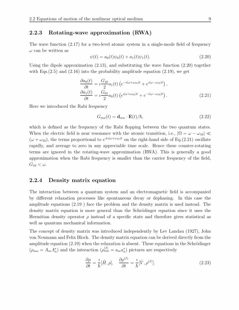
2.2.3 Rotating-wave approximation (RWA)
The wave function (2.17) for a two-level atomic system in a single-mode field of frequency
ω can be written as
ψ(t) = a0(t)ψ0(t) + a1(t)ψ1(t). (2.20)
Using the dipole approximation (2.13), and substituting the wave function (2.20) together
with Eqs.(2.5) and (2.16) into the probability amplitude equation (2.19), we get
∂a0(t)
∂t= ı
G10
2a1(t)
(e−ı(ω+ω10)t + eı(ω−ω10)t
),
∂a1(t)
∂t= ı
G01
2a0(t)
(eı(ω+ω10)t + e−ı(ω−ω10)t
). (2.21)
Here we introduced the Rabi frequency
Gmn(t) = dmn · E(t)/h, (2.22)
which is defined as the frequency of the Rabi flopping between the two quantum states.
When the electric field is near resonance with the atomic transition, i.e., |Ω = ω − ω10| (ω + ω10), the terms proportional to e±ı(ω+ω10)t on the right-hand side of Eq.(2.21) oscillate
rapidly, and average to zero in any appreciable time scale. Hence these counter-rotating
terms are ignored in the rotating-wave approximation (RWA). This is generally a good
approximation when the Rabi frequency is smaller than the carrier frequency of the field,
G10 < ω.
2.2.4 Density matrix equation
The interaction between a quantum system and an electromagnetic field is accompanied
by different relaxation processes like spontaneous decay or dephasing. In this case the
amplitude equations (2.19 ) face the problem and the density matrix is used instead. The
density matrix equation is more general than the Schrodinger equation since it uses the
Hermitian density operator ρ instead of a specific state and therefore gives statistical as
well as quantum mechanical information.
The concept of density matrix was introduced independently by Lev Landau (1927), John
von Neumann and Felix Bloch. The density matrix equation can be derived directly from the
amplitude equation (2.19) when the relaxation is absent. These equations in the Schrodinger
(ρmn = AmA∗n) and the interaction (ρ
(I)mn = ama
∗n) pictures are respectively
∂ρ
∂t=
ı
h[H, ρ],
∂ρ(I)
∂t=ı
h[V , ρ(I)]. (2.23)

10 Chapter 2 Basic theoretical tools
In the density matrix method, the radiative and nonradiative decays of the atomic or molec-
ular levels caused by spontaneous emission, collision and other phenomena can be taken into
account. The finite lifetimes of the levels are described by introducing the decay terms phe-
nomenologically into the equation (2.23),
∂ρmn
∂t=ı
h[H, ρ]mn − γmnρmn (m 6= n),
∂ρnn
∂t=
ı
h[H, ρ]nn +
∑
Em>En
Γnmρmm − Γnρnn. (2.24)
Here the diagonal matrix element ρnn gives the probability that the particle is in the energy
state n, and the off-diagonal matrix element ρmn is related to the formation of the macro-
scopic dipole moment. Γmn is the decay rate of the population from the energy level n to
m. The decay of the coherence, γmn, consists of two qualitatively different contributions,
γmn =Γm + Γn
2+ γph
mn, (2.25)
where Γi =∑
Ei′<Ei
Γi′i is the total decay rate of population out of the level i which usually
does not depend on the number density of the medium, whereas the dephasing rate γphmn is
proportional to the concentration of the molecules.
The macroscopic polarization P of the medium defined as the induced dipole moment in
unit volume is related to the ensemble average of the expectation value of the dipole moment
operator,
P = NTr(ρd), (2.26)
where N is the number density of the molecules.
2.2.5 Bloch equation
In general, the off-diagonal density matrix elements are complex quantities, contrary to the
diagonal elements which are always real. However, one can convert the complex density
matrix equations into real equations by separating the real and imaginary parts of the
elements. Assuming that ρmn = (um − ıvm)/2, m > n, where um and vm are real numbers.
Due to the Hermiticity of the density matrix operator, ρnm can then be written as (um +
ıvm)/2. Substituting them into the density matrix equations (2.24), one can obtain the
Bloch equations for these real vectors.

2.2 Equations of motion of the nonlinear optical medium 11
The Bloch equations for a closed two-level system can be written as
∂u
∂t= −γ01u− ωv +
∆d · Eh
v,
∂v
∂t= −γ10v + ωu− ∆d · E
hu+ 2
d10 · Eh
w, (2.27)
∂w
∂t= −Γ10(w + 1) − 2
d10 · Eh
v,
where ∆d = d11 − d00 is the difference of the permanent dipole moments, ρ10 = (u− ıv)/2
and w = ρ11 − ρ00 denotes the inversion of the population. The particle conservation law
ρ11 + ρ00 = 1 is used to combine the two equations for the populations into the one for
the population difference w. When a quantum system is exposed to a strong laser field,
multiphoton ionization may occurs, and the discrete-plus-continuum energy-level model
should be used then in which the photoionization can be taken into account by introducing
the time-dependent ionization rates into the density matrix or Bloch equations.

12 Chapter 2 Basic theoretical tools

Chapter 3
Numerical methods
Although analytical solutions give deep insight into the physics of the interaction of strong
laser fields with matter, it is usually difficult or impossible to solve analytically most of the
nonlinear problems that we face. One of the simplest examples is the interaction of a few-
cycle optical laser pulse with a two-level atom in which the standard approximations are not
valid anymore. In this circumstance, the strict numerical simulations become much more
efficient. In this chapter, we describe briefly the numerical techniques that are employed to
solve the coupled matter and field equations.
3.1 Crank-Nicholson method
In Section 5.1.3, we need to solve the paraxial wave equation. The Crank-Nicholson method9,10
is an important numerical method that is used to solve the parabolic type of equations, such
as the diffusion, the time-dependent Schrodinger or paraxial equations. As an example, let’s
consider the one-dimensional diffusion equation,
∂u
∂t=
∂
∂x(D
∂u
∂x). (3.1)
The Crank-Nicholson scheme of the differential equation is written as
un+1j − un
j
∆t=D
2
[(un+1
j+1 − 2un+1j + un+1
j−1 ) + (unj+1 − 2un
j + unj−1)
(∆x)2
]. (3.2)
Here, ∆t and ∆x are respectively the integration interval of t and x, and the indices (n, j)
represents the coordinate at (n∆t, j∆x). Three different numerical differencing schemes for
the diffusive problems are shown in Fig. 3.1. The Forward Time Centered Space (FTCS)

14 Chapter 3 Numerical methods
differencing scheme is first-order accurate, and stable only for sufficiently small time-steps.
The Backward Time Centered Space (BTCS) is still first-order accurate, but stable for
arbitrary large time-steps. The Crank-Nicholson scheme, which is the average of the explicit
and implicit schemes, is second-order accurate and is stable for any size of the time step.
j
n (n+1,j)
(n,j+1)(n,j)(n,j-1) (n,j)
(n+1,j+1)(n+1,j)(n+1,j-1)
(a) FTCS (b) BTCS
(n+1,j)
(n,j+1)(n,j)(n,j-1)
(n+1,j+1)(n+1,j-1)
(c) Crank-Nicholson Scheme
Figure 3.1: Three differencing schemes for diffusive problems.
With the assumption that the field is radially symmetric, in the cylindrical coordinates, the
local-time paraxial wave equation (2.11) can be written as
−ı∂E(r, z)
∂z= HE(r, z), H =
∂2
∂r2+
1
r
∂
∂r+
1
r2+k2
ε0
P
E. (3.3)
H contains the transverse derivatives and the nonlinear terms, and z = z/2k. The field
E(r, z) is replaced by E(r, z) = rE(r, z) since E(r = 0, z) = 0 can be used as one of the
boundary conditions to solve the second-order partial differential equation. Eq.(3.3) has the
same form as the time-dependent Schrodinger equation (2.14) and has a formal solution
E(r, z + ∆z) = eı eH∆zE(r, z). (3.4)
To solve the problem numerically, the exponential operator is approximated by the Cayley’s
form of finite difference, which is second-order accurate and unitary,
eı eH∆z ' 1 + 12ıH∆z
1 − 12ıH∆z
. (3.5)
Substituting Eq.(3.5) into Eq.(3.4), one can get
[1 − 1
2ıH∆z]En+1
j = [1 +1
2ıH∆z]En
j . (3.6)
Here r = j∆r, z = n∆z. Using the Crank-Nicholson scheme to replace H by its finite-
difference in r, Eq.(3.6) can always be written in the following form,
ajEn+1j+1 + bjE
n+1j + cjE
n+1j−1 = F n
j , (3.7)

3.2 Finite-difference time-domain method 15
where the coefficients
aj = 1 − 1
2j, cj = 1 +
1
2j,
bj = (∆r)2k2
ε0
P
E+
1
2j− 2 + ı
2(∆r)2
∆z, (3.8)
F nj = −ajE
nj+1 −
[bj − ı
4(∆r)2
∆z
]En
j − cjEnj−1.
Eq.(3.7) can then be solved with the techniques for the tridiagonal system of linear algebraic
equations.
3.2 Finite-difference time-domain method
The finite-difference time-domain (FDTD) method, first developed by Yee11 in 1966 is a
popular way to solve the electromagnetic field problems, which provides the electric and
magnetic fields directly as functions of time and space. Since FDTD is a time-domain
technique, already a single simulation covers a wide frequency range. This is extremely useful
in applications where resonant frequencies are not known exactly, or when a broadband
result is desired. The FDTD method is used to study the nonlinear propagation of short
optical (Chapter 5) and x-ray (Chapter 9) pulses.
By examining Maxwell’s curl equations, one can notice that the time derivative of the electric
field depends on the curl of the magnetic field, and vice verse. That is the new value of the
electric field can be determined by the old value of E and the difference in the old value
of H on either side of the electric field point in space. Therefore, the staggered leapfrog
differencing scheme of the space and time derivatives is introduced for the discretization of
the electric and the magnetic fields. Let’s explicate here the one dimensional case as an
example. Assuming that the incident field is propagating along the z axis and is polarized
along the x axis, i.e., E(r, t) = E(z, t)x and H(r, t) = H(z, t)y. The one-dimensional
Maxwell’s equations are
∂tH = − 1
µ0
∂zE , ∂tE = − 1
ε0∂zH− 1
ε0∂tP. (3.9)
The partial differential equations are discretized with the FDTD technique. The electric
field components and the magnetic field components are spatially separated by ∆z/2 and
temporally separated by ∆t/2 as shown in Fig. 3.2. The magnetic field is solved at the points
[(j + 12)∆z, (n + 1
2)∆t], and the electric field is solved at the points [(j + 1)∆z, (n + 1)∆t].

16 Chapter 3 Numerical methods
The discretized version of the Maxwell’s equations is as follows:
H(j +1
2, n+
1
2) = H(j +
1
2, n− 1
2) − ∆t
µ0∆z[E(j + 1, n) − E(j, n)],
E(j, n+ 1) = E(j, n) − ∆t
ε0∆z[H(j +
1
2, n+
1
2) −H(j − 1
2, n+
1
2)]
−ε0[P(j, n + 1) − P(j, n)]. (3.10)
n
j
(j+1/2,n+1/2)
(j,n)
(j-1/2,n-1/2)(j+1/2,n-1/2)
(j,n-1)
(j+1,n)
Figure 3.2: Staggered leapfrog differencing scheme (one-dimension Yee lattice) used for
FDTD. The magnetic components are sitting at the crossing points of the solid lines, and
the crossing points of the dashed lines are the electric components.
Due to the coupling of the Maxwell’s equations and the Bloch equations through the polar-
ization P, and the coupling of the Bloch equations along themselves, there is a mixing of the
next and the current time-step values in Maxwell-Bloch equations as one can see explicitly
from the electric field equation of (3.10). This does not allow a straightforward leap-frog
time integration. Hereby, the predictor-corrector scheme12,13 is used.
Unewi = Uold
i + ∆tFi(Unewj , Uold
j ), (3.11)
where Ui denotes the electric field components and the components of the Bloch equations,
and the functions Fi represent the parts with mixed time-step values on the right-hand
side of the equations. The set of equations (3.11) are solve iteratively until the differences
between the old and the new values of all the Ui are smaller than a specified value.
The choice of the increments ∆t in time and ∆z in space is motivated by the accuracy and
stability of the problem. In order to get results with high accuracy, ∆z must be small enough

3.2 Finite-difference time-domain method 17
comparing with either the minimum wavelength or the the smallest feature in the model.
To ensure the stability of the time-stepping algorithm, ∆z is chosen to satisfy vmax∆t ≤ ∆z,
or in three dimension
vmax∆t ≤ (1
(∆x)2+
1
(∆y)2+
1
(∆z)2)−1/2, (3.12)
where vmax is the maximum wave phase velocity in the model.
In view of the computational costs or the limited computer memories, the computational
domain must be ended at certain points in simulations of light propagation in an infinite
space. This is achieved by inserting artificial boundaries into the simulation space. The
most commonly used grid truncation techniques for open-region FDTD modeling problems
are Mur absorbing boundary condition,14 Liao boundary condition,15 and various perfectly
matched layer (PML) formulations.16,17

18 Chapter 3 Numerical methods

Chapter 4
Coherent control of quantum states
beyond RWA
Coherent control is a quantum mechanical based method for controlling dynamical processes
of atomic, molecular, or electronic systems with shaped laser pulses to obtain a desired out-
come.18–24 One of the important aspects of coherent control is to selectively populate a
particular state with a high efficiency. It is commonly believed that when a two-level sys-
tem is driven by a weak and near resonant laser field, most of the coherent phenomena
can be adequately treated within RWA,25,26 and this approximation breaks down when the
Rabi frequency is comparable with or larger than the light frequency. However, the coherent
control of a multilevel system is more complicated and the conditions for the validity of the
RWA are even more limited. In this chapter, the coherent control of populations of vibra-
tional and electronic states for multilevel systems is investigated beyond the conventional
RWA.
4.1 Coherent population of the vibrational states by a
strong IR laser pulse
The problem of population transfer in a two-level system is venerable and instructive. In
the case of zero detuning, Ω ≡ ω − ω10 = 0 , the population distribution for a two-level
system interacting with an external field can be easily obtained from Eq.(2.21) within RWA,
ρ0(t) = cos2 ϑ(t)
2, ρ1(t) = sin2 ϑ(t)
2, ϑ(t) =
t∫
−∞
|G10(t1)|dt1. (4.1)

20 Chapter 4 Coherent control of quantum states beyond RWA
Here ϑ(t) is defined as the area of the pulse. It shows that the populations ρi(t) depend on
the intensity, duration and shape of the pulse only through the pulse area.
When the photon frequency is tuned away from resonance Ω 6= 0, the evolution of the two-
level system changes qualitatively. By use of the substitution a0 = c0 exp(ı(Ω − ε)t/2) and
a1 = c1 exp(−ı(Ω + ε)t/2), Eq.(2.21) can be rewritten as
ı∂
∂t
(c0c1
)=
1
2
(Ω − ε −G10
−G01 −Ω − ε
)(c0c1
). (4.2)
When the adiabatic condition27
∆T G10Ω
(Ω2 +G210)3/2
(4.3)
is satisfied, where ∆T is the characteristic time of the change of the pulse, the time deriva-
tives of the amplitudes in Eq.(4.2) can be neglected, and the two-level system will evolve
along the adiabatic states
ψ+ =(ψ0 cos Θ + ψ1 sin Θe−ıΩt
)eı(Ω−λ)t/2, ψ− =
(ψ0 sin Θ − ψ1 cos Θe−ıΩt
)eı(Ω+λ)t/2
(4.4)
without any transition between ψ+ (ε = λ ≡√
Ω2 + |G10|2) and ψ− (ε = −λ). Here
tan 2Θ = G10/Ω, cos2 Θ = (λ + Ω)/(2λ). Apparently, the system evolves adiabatically in
the state ψ+ when it was initially in the ground state ψ(−∞) = ψ0 with Ω > 0. Contrary to
the strict resonance case (4.1), the adiabatic solution ψ± displays non-oscillatory evolution
of the populations
ρ0(t) = cos2 Θ, ρ1(t) = sin2 Θ. (4.5)
This means that the populations of the off-resonant levels will follow adiabatically the shape
of the pulse and return to the ground state when the pulse is over.
In a real multimode molecule with many vibrational states it is more difficult to design a
laser pulse to achieve a coherent excitation of the selected levels. We investigate here the
coherent control of the population of the vibrational levels in the ground electronic state
of the fixed-in-space NO molecule driven by an IR pulse (Paper I). The evolution of the
nuclear wave packet φ(t) is determined by the time-dependent Schrodinger equation
ıh∂
∂tφ(t) =
[H0 −
1
h(d ·E(t)) cos(ωt+ η)
]φ(t). (4.6)
Here d is the permanent dipole moment that depends on the nuclear distance. Eq.(4.6) is
solved numerically using the wave packet techniques without RWA and the population of

4.1 Coherent population of the vibrational states by a strong IR laser pulse 21
the vibrational state is calculated by projection of the wave packet into this state, ρν(t) =
|〈φ(t)|ν〉|2. The temporal shape of the IR pulse is modeled in the calculations as follows
I(t) = I0 exp
[− ln 2
(t− t0τ
)2m], (4.7)
where I(t) = cε0|E(t)|2/2, τ is the half width at half maximum (HWHM), t0 is the central
position of the IR pulse, I0 is the peak intensity of the IR radiation and m = 1, 2, 3,...
Figure 4.1: Dynamics of populations
of the levels ν = 0 (solid), ν = 1
(dotted) and ν = 2 (gray) of the
NO molecule for different pulse du-
rations τ and shapes (m = 1 and 3).
I0 = 2.3× 10¹² W/cm2. ω10 = 0.2376
eV. Ω = 3.4 meV. The adiabatic pa-
rameter (4.3) Ω∆T ≈ 5.2 and 2 for
m = 1 and 3, respectively. Taken
from Paper I. Reprinted with permis-
sion of Institute of Physics and IOP
Publishing Limited.
When the light frequency is tuned in strict resonance with the first vibrational transition
0 → 1 and a moderate intensity is applied to prevent excitations to higher vibrational levels,
Eq.(4.1) works well even for a many-level system. But the situation changes drastically
when the field frequency is tuned away from resonance. Fig. 4.1 shows the dynamics of the
populations for a smooth gaussian (m = 1) and a sharp “rectangular” (m = 3) pulse with
a detuning Ω = 3.4 meV. One can see that the excited state is completely depopulated at
the end of the gaussian pulse due to the big value of the adiabatic parameter |Ω|∆T ≈ 5.2.
However, the adiabatic solution breaks down for m = 3 since the adiabatic parameter
approaches one and the first-excited vibrational state is still populated after the pulse. The
above results indicate that by changing the duration, shape and intensity of the IR pulse,
one can design the vibrational wave packet of desirable form and size, due to coherently
selective population of the vibrational levels. It is worth mentioning that although there is
no population inversion caused by the adiabatic excitation of the pulse with a fixed detuning
(Fig. 4.1 (m = 1)), the system can be inverted by a chirped pulse when the frequency is
swept through the resonance slowly.27 This can be seen from Eqs.(4.4) and (4.5) when the
detuning changes adiabatically from positive to negative values. Fig. 4.1 shows that the
populations of the vibrational levels ν = 0, 1 display fast modulations with the frequency
2ω due to the breakdown of RWA.

22 Chapter 4 Coherent control of quantum states beyond RWA
4.2 Nonlinear dynamics of multilevel molecules near
two-photon resonance
4.2.1 Analytical solution beyond RWA
The two-photon interaction of laser fields with real molecular systems is one of the hot
topics of non-linear optics. Usually the dynamics of two-photon absorption (TPA) are
studied for few-level systems within RWA or RWA with zero dynamical Stark shift (RWAZS).
The importance of the two-photon dynamical Stark shift has been pointed out in many
publications and was studied extensively.28–34 However, the strict analytical treatment of
the problem beyond RWA is absent according to our knowledge.
2
0
m
...
Figure 4.2: Multilevel scheme of two-photon absorption transition. Taken from Paper II.
Reprinted with permission of American Physical Society.
We considered here the two-photon interaction between multilevel molecules and linearly
polarized light E(z, t) = E(z, t) cos(ωt − kz + η), where η is the phase of the pulse. The
light is tuned near two-photon resonant transition 0 → 2 (see Fig. 4.2) with the detuning δ
much smaller than the frequency ω of the light, δ = 2ω − ω20, |δ| ω. The duration τ
of the pulse is assumed to be shorter than the relaxation times of the excited states. This
allows us to neglect the relaxation rates and to use amplitude equations instead of the more
complicated density matrix formalism. The laser field creates a coherent superposition of
molecular states ψ(t) =∑m
am(t)ψm with am(t) = Am(t) exp(ıωm0t). The mixing coefficients
obey the amplitude equations (2.19). The intermediate states are assumed to be far away
from resonance. Eqs.(2.19) are solved beyond RWA using the Fourier transformation of the
amplitudes (see details in Paper II). The SVEA together with the assumption that the Rabi
frequency is smaller than the one-photon detuning Ω ≡ ω − ωm0,
|Ω|τ, |Ω/η| 1, ζ ≡(Gmi
4ω
)2
1, i = 0, 2, (4.8)
allows us to keep only the time derivatives of the amplitudes near resonance. Hence, the
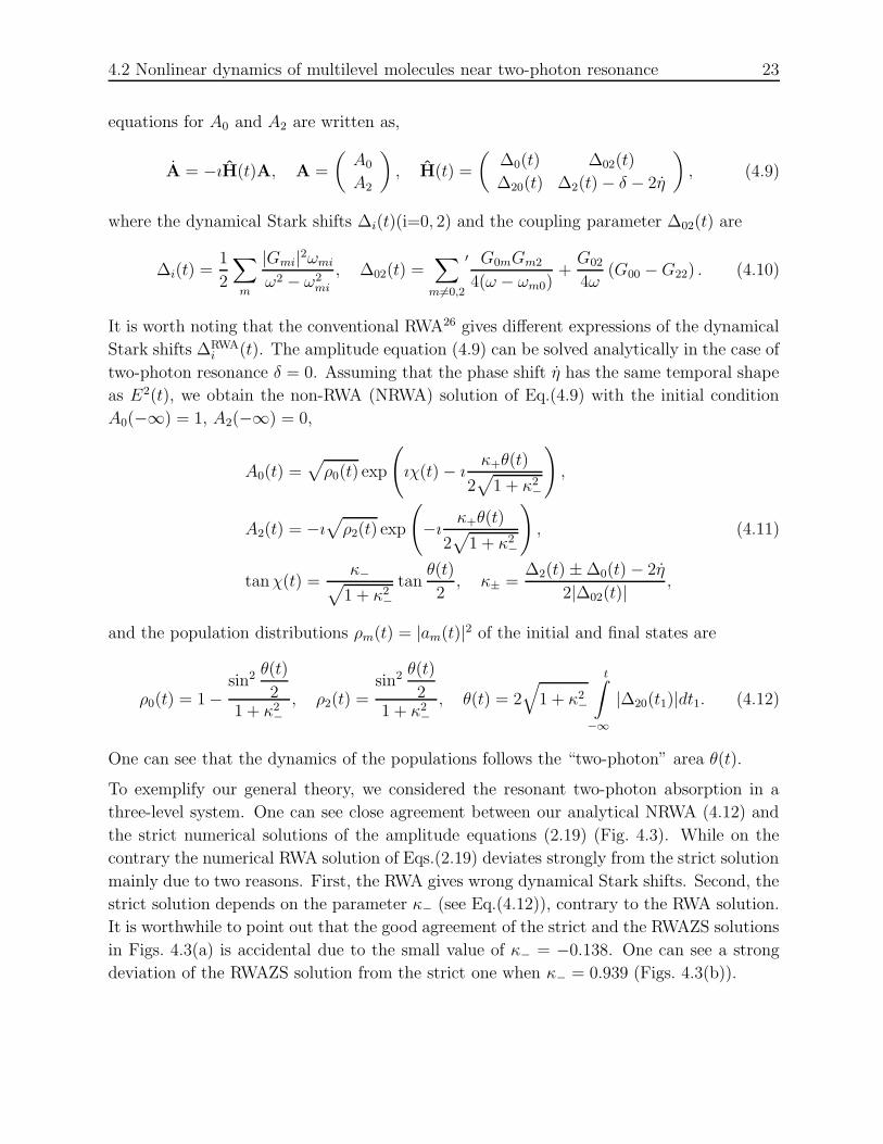
4.2 Nonlinear dynamics of multilevel molecules near two-photon resonance 23
equations for A0 and A2 are written as,
A = −ıH(t)A, A =
(A0
A2
), H(t) =
(∆0(t) ∆02(t)
∆20(t) ∆2(t) − δ − 2η
), (4.9)
where the dynamical Stark shifts ∆i(t)(i=0, 2) and the coupling parameter ∆02(t) are
∆i(t) =1
2
∑
m
|Gmi|2ωmi
ω2 − ω2mi
, ∆02(t) =∑
m6=0,2
′ G0mGm2
4(ω − ωm0)+G02
4ω(G00 −G22) . (4.10)
It is worth noting that the conventional RWA26 gives different expressions of the dynamical
Stark shifts ∆RWAi (t). The amplitude equation (4.9) can be solved analytically in the case of
two-photon resonance δ = 0. Assuming that the phase shift η has the same temporal shape
as E2(t), we obtain the non-RWA (NRWA) solution of Eq.(4.9) with the initial condition
A0(−∞) = 1, A2(−∞) = 0,
A0(t) =√ρ0(t) exp
(ıχ(t) − ı
κ+θ(t)
2√
1 + κ2−
),
A2(t) = −ı√ρ2(t) exp
(−ı κ+θ(t)
2√
1 + κ2−
), (4.11)
tanχ(t) =κ−√
1 + κ2−
tanθ(t)
2, κ± =
∆2(t) ± ∆0(t) − 2η
2|∆02(t)| ,
and the population distributions ρm(t) = |am(t)|2 of the initial and final states are
ρ0(t) = 1 −sin2 θ(t)
21 + κ2
−
, ρ2(t) =sin2 θ(t)
21 + κ2
−
, θ(t) = 2√
1 + κ2−
t∫
−∞
|∆20(t1)|dt1. (4.12)
One can see that the dynamics of the populations follows the “two-photon” area θ(t).
To exemplify our general theory, we considered the resonant two-photon absorption in a
three-level system. One can see close agreement between our analytical NRWA (4.12) and
the strict numerical solutions of the amplitude equations (2.19) (Fig. 4.3). While on the
contrary the numerical RWA solution of Eqs.(2.19) deviates strongly from the strict solution
mainly due to two reasons. First, the RWA gives wrong dynamical Stark shifts. Second, the
strict solution depends on the parameter κ− (see Eq.(4.12)), contrary to the RWA solution.
It is worthwhile to point out that the good agreement of the strict and the RWAZS solutions
in Figs. 4.3(a) is accidental due to the small value of κ− = −0.138. One can see a strong
deviation of the RWAZS solution from the strict one when κ− = 0.939 (Figs. 4.3(b)).

24 Chapter 4 Coherent control of quantum states beyond RWA
0
50
100
0 2 4 6-100
-50
0
50
100
0 2 4 6
(a1)
ρ 2 (%)
1
2
3 3
1
2
(b1)
1 NRWA 2 RWA 3 RWAZS
2
3
(a2)
ρstric
t2
-ρl 2 (%
)
θ(t)/π
1
θ θ
3
12
(b2)
θ(t)/π
Figure 4.3: Comparison of the NRWA
(4.12) (solid), RWAZS (dashed), and
RWA (dash-dotted) solutions with the
strict numerical solution (filled circles)
of the amplitude equations (2.19). (a)
κ− = −0.138, G10 = 0.127eV, G12 =
0.225 eV and (b) κ− = 0.939, G10 =
0.193 eV, G12 = 0.109 eV. ω10 = 3.46
eV, ω20 = 4.27eV. ω = 2.135 eV, τ =
0.5 ps. Taken from Paper I. Reprinted
with permission of Institute of Physics
and IOP Publishing Limited.
Since our NRWA solution (4.12) is based on the condition (4.8), it starts to break down
when a short pulse is strong enough and Gij/ω ∼ 1 (Fig. 4.4). The analytical solution fails
to describe the non-RWA modulations35 with the frequency 2ω. Also, the strict numerical
solution shows rather high population of the intermediate state and shift of the extrema of
ρ2 relative to the analytical result (4.12). This means that higher order non-RWA terms
((Gij/ω)2, (Gij/ω)3, · · · ) have to be taken into account when Gij/ω ∼ 1.
0 1 2 3 40
50
100
ρ1
Popu
latio
n(%
)
θ(t)/π θ π
ρ2
Figure 4.4: Break down of the NRWA
solution (4.12). Solid and dashed lines
show the population ρ2 obtained from
the strict numerical and NRWA (4.12)
solutions, respectively. Input data are
the same as in Fig. 4.3(a) except for
τ = 25 fs and I0 = 6.055×10¹¹ W/cm2.
Taken from Paper II. Reprinted with
permission of American Physical Soci-
ety.
4.2.2 Compensation of dynamical Stark shifts by phase tailoring
and detuning
As one can see from Eq.(4.12), the maximum value of the upper state population, ρmax2 =
1/(1 + κ2−), can be achieved when the two-photon area of the incident pulse equals to odd
4.2 Nonlinear dynamics of multilevel molecules near two-photon resonance 25
multiples of π. When η = δ = 0 the dynamical Stark shift does not allow 100% population
of the excited state because in general case ∆0 6= ∆2 and hence κ− 6= 0. However, one can
compensate the dynamical Stark shift by special tailoring of the phase of the pulse,22
η(t) =1
2(∆2(t) − ∆0(t)) . (4.13)
Using the phase tailoring technique, the upper state can be fully populated with π, 3π, · · ·pulses defined by Eq.(4.12).
The population transfer can also be optimized by a proper detuning δ from the two-photon
resonance,22 because in general case κ− is a function of both the detuning and the phase of
the pulse, and can be expressed approximately as
κ−(t) =∆2(t) − ∆0(t) − 2η − δ
2|∆02(t)| , (4.14)
even though it is difficult to give a precise expression of the pulse area in the case of
nonzero detuning from the two-photon resonance. With a proper two-photon detuning, one
can compensate completely the side effect caused by the dynamical Stark shifts and get
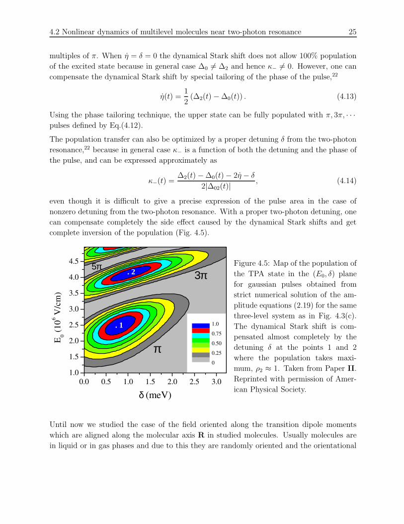
complete inversion of the population (Fig. 4.5).
0.0 0.5 1.0 1.5 2.0 2.5 3.01.0
1.5
2.0
2.5
3.0
3.5
4.0
4.5 5π3π
. 1
δ (meV)
E 0 (106 V
/cm
)
0
0.25
0.50
0.75
1.0
. 2
π
Figure 4.5: Map of the population of
the TPA state in the (E0, δ) plane
for gaussian pulses obtained from
strict numerical solution of the am-
plitude equations (2.19) for the same
three-level system as in Fig. 4.3(c).
The dynamical Stark shift is com-
pensated almost completely by the
detuning δ at the points 1 and 2
where the population takes maxi-
mum, ρ2 ≈ 1. Taken from Paper II.
Reprinted with permission of Amer-
ican Physical Society.
Until now we studied the case of the field oriented along the transition dipole moments
which are aligned along the molecular axis R in studied molecules. Usually molecules are
in liquid or in gas phases and due to this they are randomly oriented and the orientational

26 Chapter 4 Coherent control of quantum states beyond RWA
averaging over the angle γ = 6 e,R between the polarization vector e of the field and the
molecular axis is needed (see Paper I). The orientational disorder reduces the efficiency
of population transfer to the upper state, and a complete compensation of the dynamical
Stark shift is much more difficult for the randomly oriented molecules. But on the other
hand, the orientational selectivity of photo-excitation can have important applications in
photochemistry processes such as photobleaching.
4.2.3 Anisotropy of photobleaching
Quite often molecules are damaged in excited states because of the photochemical reactions
that remove the molecules from the absorption-emission cycle.36,37 The two-photon induced
photobleaching can be used as the recording mechanism in optical memory materials shined
by a sequence of short laser pulses because it reduces the number of intact molecules Nintact
∂Nintact
∂t= −N2
τ 0B
, N2 = ρ2(t)Nintact =sin2( θ
2cos2 γ)
1 + κ2−
Nintact. (4.15)
For randomly oriented molecules, the substitution ∆i → ∆i cos2 γ, ∆02 → ∆02 cos2 γ, θ(t) →θ(t) cos2 γ is used in ρ2(t) (4.12). The solution of this equation
ρintact(γ, t) = exp
(− t
τBsin2(
θ
2cos2 γ)
)(4.16)
is shown in Fig. 4.6. Here 1/τ 0B is the rate of photobleaching, θ = θ(∞) and τB = τ 0
B(1+κ2−).
Fig. 4.6 shows that the light “removes” the molecules aligned along the field γ ≈ 00, 1800.
Thus the reading is possible only by a field with the same polarization as the writing one.
0 45 90 135 1800
50
100
0
50
100
0
50
100
ρ inta
ct(%
)
γo
∆γ
180o
ρ inta
ct(%
)
∆γ
e 00
90o
Figure 4.6: Selectivity of photobleaching for randomly oriented molecules, t/τB = 5. θ = π/2.
Taken from Paper I. Reprinted with permission of Institute of Physics and IOP Publishing Limited.

Chapter 5
Pulse propagation: short versus long
pulses
Varieties of nonlinear optical phenomena are generated during the propagation of laser
pulses in optical media. Owing to the propagation effects, the temporal and spatial shapes
of the pulse as well as its spectral distributions will be modified. Generally speaking, when
the propagation of a long pulse is considered, SVEA (see Eq.(2.6)) and RWA (see Sec. 2.2.3)
are valid, and it is possible to get instructive analytical solutions. Nevertheless, SVEA and
RWA break down due to the short duration and the strong intensity of a short pulse. In
this case, numerical simulations become the main theoretical tools for the investigation of
pulse propagation. In this chapter, we study both analytically and numerically some of the
nonlinear optical effects that occur when laser pulses propagate through media with strong
nonlinear optical properties.
5.1 Two-photon induced optical power limiting
The fast development in modern laser technology makes it possible to generate extremely
intense and short laser pulses, which pose a potential hazard for eyes and optical sensors.
Therefore, optical power limiting has attracted great attention because of the needs for
automatic protection of optical sensors against intense laser radiation. It is known that sev-
eral nonlinear mechanisms can lead to optical limiting behavior, such as reverse saturable
absorption,38–40 two-photon absorption,41–44 nonlinear refraction, and optically induced scat-
tering.45 In this section, we focus our attention on the study of optical limiting performance
induced by the two-photon processes, including one-step TPA and two-step TPA.

28 Chapter 5 Pulse propagation: short versus long pulses
5.1.1 Pulse propagation and two-photon area theorem
When the propagation of a laser pulse in an optically resonant material is investigated, the
”pulse area” language can describe very easily the interesting nonlinear optical phenomena,
such as self-induced transparency, pulse splitting and pulse compression. The area theorem
for resonant one-photon interaction in a two-level atomic medium was first derived by McCall
and Hahn in 1967.46 Based on SVEA and RWA, McCall and Hahn found that when the
damping of the system is negligibly small during the time of interaction, the evolution of
the pulse area (2.21) obeys the following equation,47
d
dzϑ(z) = −1
2α sin ϑ(z), (5.1)
where α = 4π2Nωd210/hc is the absorption coefficient.
We derive here for the first time the ”two-photon area theorem” (Paper III) which describes
the evolution of the two-photon area (4.12) for resonant two-photon interaction in a mul-
tilevel molecular medium by use of the non-RWA solution in Chapter 4. Substituting the
non-RWA solution of the amplitude equations (4.11) into the polarization (2.26) and the
field equation (2.7), one can get(∂
∂z+
∂
c∂t
)θ(z, t) = − 2
Lsin2 θ(z, t)
2. (5.2)
Here L = ε0h√
1 + κ2−/(4Nk|γ02|) with γ02 = h2∆02(z, t)/E2(z, t), and κ− is defined by
Eq.(4.11). The two-photon area theorem which takes account of the non-RWA effects is
obtained directly from Eq.(5.2) when t→ ∞,
d
dzθ(z) = − 2
Lsin2 θ(z)
2. (5.3)
The solution θ(z) of the area equation (5.3) is a step-like function confined in the region
2(n− 1)π < θ(z) < θ(z0),
θ(z) = θ(z0) + 2
[arccot
(z − z0 − zc
L
)− arccot
(−zc
L
)], (5.4)
where θ(z0) is the initial area of the pulse at the entry z0 of the medium and 2(n − 1)π <
θ(z0) < 2nπ, n ≥ 1 and 0 ≤ arccotx ≤ π. The length zc = −L cot(θ(z0)/2) characterizes
the distance of enhanced optical limiting during pulse propagation.
In the derivation of the area theorem, the SVEA with 1/τ ω is used and also all the
relaxation rates are neglected in which the dephasing rate γ is the largest one. Therefore,
the area theorem [Eq.(5.3) and Eq.(5.4)] is applicable under the following conditions,
γ 1
τ ω. (5.5)

5.1 Two-photon induced optical power limiting 29
It is worth noting that the one-photon pulse area (2.21) is the time integral of the pulse
envelope, and along propagation it can either be decreased or increased (Fig. 5.1 (a)).
However, the two-photon area (4.12) is the time integral of the pulse intensity, which is
proportional to the energy fluence of the pulse, therefore it can not be increased when it
propagates in an absorbing medium (Fig. 5.1 (b)).
(b)2n
2n-1(z)/
z2(n-1)
(a)
(z)/
z
2n-1
2(n-1)
2n
Figure 5.1: Schematic representation of (a) McCall-Hahn one-photon area theorem (5.1)
and (b) our two-photon area theorem (5.3). n=1,2,· · · .
5.1.2 Optical limiting of short laser pulses
The optical limiting properties of a short laser pulse propagating two-photon resonantly in
a medium can be investigated from the point of view of two-photon area (energy fluence).
Fig. 5.2 shows the TPA induced optical limiting behavior at different distances obtained
directly from the two-photon area theorem (5.4). It is necessary to note that the two-photon
area theorem can be used only when the field is not very strong and the propagation distance
is short enough. This is because it considers only the main field with frequency ω and ignores
other new frequency components generated during interaction, such as harmonic generation,
superfluorescence (SF), amplified spontaneous emission (ASE), four-wave mixing (FWM)
and other frequency components. However, the area theorem can be useful in analyzing
pulse propagation accompanied by generation of fields with new frequencies.
Strict numerical results, which take into account all these new fields generated along pulse
propagation, for the two-photon resonant propagation of ultrashort laser pulses in a sym-
metric NLO material are also shown in Fig. 5.2 (discussed in details in Sec. 5.2.1). What’s
surprising is that the area theorem (5.4) and the strict numerical solution of the coupled
Maxwell-Bloch equations for the ultrashort pulse show rather similar behaviors. The system

30 Chapter 5 Pulse propagation: short versus long pulses
is almost transparent at low laser intensity, but becomes increasingly opaque as the two-
photon area is increased. The step-like behavior of the area θ(z) near θ(0) = 2π (Fig. 5.2)
predicted by the two-photon area theorem takes place also in real cases. The area theorem
explains qualitatively the evolution of the ultrashort pulses, although the change of the slope
of the optical limiting curve is not as strong as shown by the area theorem.
0 1 2 3 40
1
2
3
4
0 1 2 3 40
1
2
3
4
0.0 0.1 0.2 0.3 0.4 0.50.0
0.1
0.2
1µm 3µm 10µm
θ(z)
/π
θ(0)/π
2.5fs 7.0µm 7.5fs 7.0µm
Figure 5.2: Output area of the pulse θ(z) versus input pulse area θ(0). The curves are
calculated using the area theorem (5.4) except for those with τ = 2.5 fs and τ = 7.5 fs
which are computed by the strict numerical solution of the coupled Maxwell-Bloch equations.
Taken from Paper III. Reprinted with permission of American Physical Society.
5.1.3 Optical limiting of long laser pulses
Coherent and incoherent two-photon absorption
In the previous section, we discussed the optical limiting of short laser pulses induced by
the coherent one-step TPA. Actually, it is well established that there are two qualitatively
different TPA processes: coherent one-step TPA in which two photons are absorbed simul-
taneously by the TPA state (Fig. 5.3 (a)) and incoherent two-step (sequential) TPA via
one-photon off-resonant population of the intermediate state (Fig. 5.3 (b)). Both of them
may contribute in nonlinear absorption processes. These two mechanisms of TPA can be
separated by variation of the pulse duration because of the instantaneous nature of one-step

5.1 Two-photon induced optical power limiting 31
TPA in contrast to the two-step TPA which has a finite response caused by the finite rate
of population of the intermediate states.
The triplet state plays an exceptional role in sequential TPA because of its long lifetime
(∼ 1µs− 1ms). When the duration of the pulse is comparable to or longer than the time
of population transfer into the triplet state, the population of the ground state can be
transferred almost completely to the triplet state by a rather weak field if the lifetime of
the triplet state is also long. Consequently, the sequential (singlet-singlet)×(triplet-triplet)
absorption can result in nonlinearities even in a rather weak field. On the contrary, the
one-step nonlinear absorption in the case of long pulses is very weak because of its small
peak intensity in comparison with the short laser pulses.
f
g
(a)
f
g
i
(b)
Figure 5.3: Scheme of TPA. (a) One-step TPA; (b) Two-step TPA.
Optical limiting performance of fullerene C60 for microsecond pulses
We consider the interaction of nonlinear media with long pulses in the microsecond time
domain by use of the generalized five-level model (Fig. 5.4) and the fullerene C60 molecule
is selected to exemplify the general theory (Paper IV). The key features of C60 are its broad
spectral induced absorption, rather fast rate of intersystem crossing, long lifetime of the
triplet state, and rather weak ground state absorptions, all of which make this material an
interesting candidate for application of optical power limiting.
The system studied has different time scales, and can be divided into fast and slow subsys-
tems. The relaxation rates of the excited singlet (ΓS1+γc ∼ ns, ΓSn ∼ ps) and triplet (ΓT2 ∼ps) states are the faster ones, while the dynamics of the ground and the lowest triplet states
are the slower ones and are characterized by the duration of the pulse τ ∼ µs and by the
time τST of population transfer between these two states. The short lived quantum states
follow adiabatically the slow dynamics of the laser field and the populations of the ground
and the first-excited triplet states. This makes valid the adiabatic solutions for the excited
singlet states and the higher triplet states. Combining these adiabatic solutions and the

32 Chapter 5 Pulse propagation: short versus long pulses
γc
ΓT1
ΓT2
ΓS1
T1
T2iSni
S1S1
S0
ΓSn
Figure 5.4: Jablonski diagram for fullerene C60.
particle conservation law with the rate equation for the ground state population, one can
reduce the coupled rate equations of the multilevel system to a single dynamical equation
for the ground state population,
∂
∂tρS0 = −γ0(t)ρS0 + ΓT1P (t) =
q(t) − ρS0
τST (t), (5.6)
where q(t) = τST (t)ΓT1P (t). The dynamics of depopulation of the ground state is defined
by the time of population transfer between S0 and T1 levels
τST (t) =1
γ0(t), γ0(t) = γ(t)Φ(t) + ΓT1Q(t). (5.7)
Here P (t) and Q(t) are some time-dependent factors related to the probabilities of field
induced decays. The first term on the right-hand side of Eq.(5.7) of γ0(t) has a simple
physical meaning, namely that the population transfer S0 → T1 is equal to the pump rate
γ(t) = σI(t)/hω times the probability of intersystem crossing Φ(t) = γc/(ΓS1 + γc + γ(t)).
The denominator of Φ(t) is the total rate of depopulation of the S1 level, and σ is the
one-photon absorption cross section.
The pulse propagation is studied by solving numerically the paraxial field equation (2.11)
in the local time frame with the Crank-Nicholson method outlined in Sec. 3.1 together with
the effective rate equation (5.6) for the ground state. The transverse inhomogeneity of the
laser field is taken into account, and the initial pulse with a Gaussian distribution is used,
E(r, z0, T0) = E0(T0)w0
w(z0)exp
(− r2
w2(z0)
)exp
(ik
r2
2R(z0)− iζ(z0)
), (5.8)
where w(z) = w0
√1 + (z/l0)2 is the beam width at the point z, l0 = πw2
0/λ is Rayleigh
length, R(z) = z [1 + (l0/z)2], and ζ(z) = arctan(z/l0). The temporal shape of the incident
pulse is also modeled by a gaussian (Eq.(4.7), m = 1). A semi-empirical expression of the

5.1 Two-photon induced optical power limiting 33
polarization by using the experimental cross sections of one-photon absorptions is used,
instead of the full ab-initio calculations (2.26).
The main mechanism of optical limiting for long pulses is the sequential (singlet-singlet) ×(triplet-triplet) two-photon absorption, whose performance is related to the large population
of the lowest triple state and the strong one-photon absorption of the triple states. When
the light intensity is high enough, the ground state is depopulated and most of its population
is accumulated at the lowest triplet state because of its long lifetime. An efficient optical
limiting performance requires a much higher one-photon absorption cross section of the
triplet state compared with the ground state. The experimental data48 shows that such a
requirement is very sensitive to the wavelength. A different optical limiting behavior can
be obtained by tuning the wavelength.
0
5
10
0 5 10
1.02.03.04.0
5.06.0
7.08.0
9.0
10
1 2 3 4
0.5
1.0
1.5
2.0
2.5
3.0
t (µs)
r (m
m)
0 2.0 4.0 6.0 8.0 10 12
I (r,
L/2
, t) (
KW
/cm
2 )
r=0.03 mm r=1.0 mm r=1.5 mm
t=0.9 µs t=1.5 µs t=2.0 µs
I (r, L/2, t) (KW/cm2)
Figure 5.5: 2D map of the output field intensity after passing through the absorbing medium
centered at z=0 (L = 1.0 mm). The concentration of C60 is N = 1020 cm−3. λ = 650 nm,
w0 = 1.0 mm, I0=10 MW/cm2, τ = 0.5µs, t0 = 2.0µs. Taken from Paper IV. Reprinted
with permission of American Institute of Physics.
The dynamics of populations and of pulse propagation are characterized mainly by the time
of population transfer between the ground and the lowest triplet states. This time decreases
with the increase of field intensity. Therefore the front part of the pulse propagates mainly

34 Chapter 5 Pulse propagation: short versus long pulses
with linear absorption, while the main body of the pulse is significantly attenuated due to
the strong nonlinear sequential two-photon absorption (Fig. 5.5). The nonlinear absorption
starts from S0 → S1 linear absorption where the energy transmittance of the pulse equals
to TS0S1 = exp(−NσL). The absorption increases with the increase of the field intensity
because of the population of the lowest triplet state and the strong T1 → T2 linear absorption.
The transmittance is saturated and approaches the lowest limit TT1T2 = exp(−NσTL) when
the population of the T1 level is close to 1 at high intensities. The incident pulse with a
gaussian transverse distribution is strongly absorbed near the axis due to the higher initial
intensity there, which results in a hole in the radial distribution of the pulse shown clearly
in Fig. 5.5. The propagation effect also plays a very important role in the optical limiting
performance of the medium. During propagation the field intensity as well as the population
of the triplet state decreases which means that the nonlinear two-step TPA is weakened and
the linear one-photon absorption gradually dominates for thick absorbers.
5.2 Propagation of ultrashort laser pulses
5.2.1 Superfluorescence and amplified spontaneous emission
The cooperative effects involve many inverted atoms and change the nature of the spon-
taneous emission.49–56 The inverted medium can radiate its energy through typically two
different ways: one is superfluorescence (SF), and the other is amplified spontaneous emis-
sion (ASE). SF is non-stationary emission, where the formation and growth of the macro-
scopic dipole moment is expected. In contrast, ASE is quasi-stationary emission, where
the formation of the macroscopic dipole moment is prevented due to the fast dephasing
of coherence between individual dipole. A full quantum mechanical description50–52 of the
Maxwell-Bloch equations based on SVEA and RWA shows that the peak intensity of SF
is proportional to the square of the number of emitters Nt, and the duration of the SF
is proportional to the reciprocal of the number of emitters, and the delay time between
SF and the excitation pulse decreases with the increase of the atomic number density, i.e.,
ISF ∝ N2t , τSF ∝ 1/Nt, τD ∝ 1/Nt. On the contrary, there is no delay between the emission
and the excitation fields and the peak intensity no longer scales as N 2t in ASE.53
We investigate the dynamics of cooperative emissions in the 4, 4’-bis(dimethylamino) stil-
bene (Paper V). The cascade three-level model is used and the incident ultrashort laser
pulse is tuned in two-photon resonance with the transition between the lowest and the up-
permost levels. The full-wave Maxwell-Bloch equations without SVEA and RWA are solved
numerically by use of the iterative predictor-corrector FDTD method outlined in Sec. 3.2.
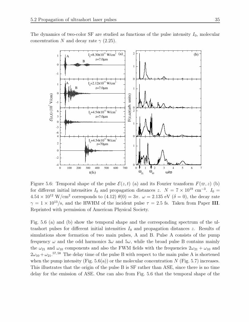
5.2 Propagation of ultrashort laser pulses 35
The dynamics of two-color SF are studied as functions of the pulse intensity I0, molecular
concentration N and decay rate γ (2.25).
-1
0
1
0
1
2
-1
0
1
0
1
-6
-3
0
3
6
0
1
2
0 100 200 300 400 500 600 700-4
-2
0
2
4
0 1 2 3 4 5 6 70
1
z=7.0µmBA
(a)I0=8.30x10¹¹ W/cm2 (b)
z=7.0µmI0=2.12x10¹² W/cm2
AB
F(z,
ϖ)(a
rb. u
nits)
I0=4.54x10¹² W/cm2
(z
,t) (1
07 V/c
m)
z=7.0µm
z=70µmI0=4.54x10¹² W/cm2
t(fs) ω10
ω21
ϖ/ω
Figure 5.6: Temporal shape of the pulse E(z, t) (a) and its Fourier transform F ($, z) (b)
for different initial intensities I0 and propagation distances z. N = 7 × 1019 cm−3. I0 =
4.54 × 10¹² W/cm2 corresponds to (4.12) θ(0) = 3π. ω = 2.135 eV (δ = 0), the decay rate
γ = 1 × 10¹³/s, and the HWHM of the incident pulse τ = 2.5 fs. Taken from Paper III.
Reprinted with permission of American Physical Society.
Fig. 5.6 (a) and (b) show the temporal shape and the corresponding spectrum of the ul-
trashort pulses for different initial intensities I0 and propagation distances z. Results of
simulations show formation of two main pulses, A and B. Pulse A consists of the pump
frequency ω and the odd harmonics 3ω and 5ω, while the broad pulse B contains mainly
the ω21 and ω10 components and also the FWM fields with the frequencies 2ω21 + ω10 and
2ω10 +ω21.57,58 The delay time of the pulse B with respect to the main pulse A is shortened
when the pump intensity (Fig. 5.6(a)) or the molecular concentration N (Fig. 5.7) increases.
This illustrates that the origin of the pulse B is SF rather than ASE, since there is no time
delay for the emission of ASE. One can also from Fig. 5.6 that the temporal shape of the

36 Chapter 5 Pulse propagation: short versus long pulses
pulse as well as its spectrum depends strongly on the intensity and propagation depth. The
increase of the intensity results in an enhancement of the harmonic generation. The total
field can not be separated into parts A and B when the pump intensity is high enough or
when z is too large. During propagation the energy of the pump field is transferred almost
completely into harmonics and SF fields. One can see the complete quenching of the 1 → 0
SF field, red shift of the third harmonic, and strong deformation of the spectral band near
the pump frequency ω at z = 70µm.
The temporal shape of the field after propagating 7.0µm in the medium with different
concentrations is shown in Fig. 5.7. With the increase of the molecular number density,
the intensities of the cooperative emissions are enhanced, and the delay times between the
cooperative emissions and the excitation pulse are decreased.
-3
0
3
-3
0
3
0 100 200 300 400 500 600
-3
0
3
-3
0
3
N=7x1018 cm-3
N=7x1019 cm-3
(z
,t) (1
07 V/c
m)
N=7x1020 cm-3
t (fs)
N=7x1017 cm-3
delay time
superfluorescence
Figure 5.7: Temporal shape of a 1.4π pulse after propagating 7.0µm in the medium for
different molecular number densities. ω = 2.135 eV, γ = 1× 10¹³/s, τ = 2.5 fs. Taken from
Paper V. Reprinted with permission of Chinese Physical Society.

5.2 Propagation of ultrashort laser pulses 37
5.2.2 Supercontinuum generation
Supercontinuum generation (SCG) refers to the extreme broadening of an optical spectrum
as it passes through an optical medium. This phenomenon was first observed in 1970,59 and
since then it has been observed in many different solids, liquids, and gases under a wide
variety of experimental conditions. When an intense laser pulse propagates in the nonlinear
medium, FWM, SRS, self-phase modulation (SPM),1 high harmonic generation (HHG),60,61
etc., lead to strong modulation of the spectrum of the field. It is generally believed that
SPM is the dominant process when the continuum emission is involved59,62–64 during the
one-photon resonant propagation of the pulse in a two-level system. Because during the
resonant propagation of a pulse with its initial area ϑ larger than 3π, the pulse will be
splitted into sub-pulses. Furthermore, the foregoing sub-pulse will be compressed and has
a higher intensity. The steepening of the pulse increases the time derivative of the pulse
intensity and results in broadening of the field spectrum.1
We investigate here the one-photon resonant propagation of few-cycle laser pulses in a
dipolar molecular medium by use of a generalized two-level model (Paper VI). For a few-
cycle laser pulse, the carrier-envelope phase (CEP) becomes important in the interaction
with medium.65,66 And when the pulse intensity is high enough, photoionization of the
quantum system takes place. Therefore, the roles of CEP and time-dependent ionization
on SCG should be considered. We solve numerically here the one-dimensional full-wave
Maxwell’s (3.9) and Bloch equations (2.27) for the two-level-plus-continuum system using
the iterative predictor-corrector FDTD technique outlined in Sec. 3.2.
The spectra of ultrashort pulses with different initial pulse areas ϑ (4.1) propagating reso-
nantly (ω = ω10) in a dipolar medium with a difference of the permanent dipole moments
∆d = d11 − d00 = 2.59× 10⁻²⁹ C.m are shown in Fig. 5.8(a). One can clearly see the forma-
tion of high spectral components and the oscillatory features around the resonant frequency.
The spectral features of the high spectral components depend strongly on the initial pulse
area ϑ. A larger pulse area results in more high spectral components which will become
distinguishable peaks caused by the strong interference between the sub-pulses. The spec-
tral analysis of each sub-pulse after splitting of the incident pulse approves that the SCG is
mainly due to the SPM of the foregoing sub-pulse. Fig. 5.8(a) also shows that the CEP has
an obvious influence on the spectra of the fields. This is because different CEP gives rise to
different intensity distribution of the carrier field and results in a different SPM effect.
Since the incident pulse with a large area is splitted and the foregoing sub-pulse is compressed
during the resonant propagation, it is possible to generate a pulse much shorter than the
incident one. The intensity distribution of the foregoing sub-pulse at different propagating
distances in nondipolar and dipolar media is shown in Fig. 5.8(b). One can see that the

38 Chapter 5 Pulse propagation: short versus long pulses
foregoing sub-pulse is strongly compressed in both the dipolar and nondipolar cases, and a
75 attosecond sub-pulse (HWHM) is generated in the dipolar medium. Generally speaking,
the permanent dipole moments can lead to either constructive or destructive effects on the
formation of the attosecond pulse, depending on its value relative to the transition dipole
moment.
0 1 2 3 4 5 6 70
5
10
0
5
10
0
5
10
phase=0 phase=π/2
ϑ=12
|(
)| (a
rb.u
nits)
ϑ=8
ϑ=6
(a)
0 1 2 30.0
0.5
1.0
1.5
0.0
0.5
1.0
1.5
0.0
0.5
1.0
1.5
2.0
z=20µm
∆t (fs)
150 as
∆d ∆d= 0
inte
nsity
(arb
.uni
ts)z=12µm
z=8µm
(b)
Figure 5.8: (a) Spectra of the ultrashort pulses in a dipolar medium with ∆d = 2.59× 10⁻²⁹ C.m
at z = 16µm. (b) Temporal shape of the foregoing sub-pulse for the incident 6π pulse with a zero
initial CEP. ∆d = 2.59 × 10⁻²⁹ C.m (solid lines) and 0 C.m (dash-dot lines). The HWHM of the
input pulses is τ = 1 fs. ω = ω10 = 3.05 eV. Taken from Paper VI. Reprinted with permission of
Institute of Physics and IOP Publishing Limited.
As far as ionization is concerned, if the rate of ionization is not very high, it mainly weakens
the oscillating feature of the basic spectral component due to the reduction of interference
between the sub-pulses, and has little influence on the higher spectral components as they
are basically produced by the SPM of the foregoing sub-pulse. However, stronger ionization
weakens obviously the intensity of the forgoing attosecond sub-pulse as well as the intensity
of the high spectral components.

Chapter 6
Multimode resonant Auger scattering
from the ethylene molecule
X-rays have wavelengths from hundreds of Angstrom to tenths of an Angstrom with at-
tosecond to subattosecond time structures. X-ray spectroscopy is one of the main methods
for understanding the atomic and electronic structures of matter2 and for studying the fast
nuclear dynamics.67 Ultrashort x-ray pulses give opportunities to explore even attosecond
electronic dynamics.68 Linear and nonlinear interactions of x-rays with molecules will be
investigated in the following chapters. We will start from the scattering of weak x-ray ra-
diation and consider resonant Auger scattering (RAS) in this chapter. The RAS process is
very similar to resonant Raman scattering (RRS) except for the final particles which are
Auger electrons instead of the scattered x-ray photons as in RRS.67
6.1 Scheme of transitions and vibrational modes
We consider the RAS of C2H4 molecules (Fig. 6.1)
ω + |0〉 → |1b−11u 1b2g〉 → |1b−1
3u 〉 + e− (6.1)
with the final state X2B3u = |1b−13u 〉, and the ground state
|0〉 = |X1Ag〉 = (1ag)2(1b1u)2 · · · (1b2u)2(3ag)2(1b3g)2(1b3u)2. (6.2)
This molecule was studied earlier using photoelectron spectroscopy .69 Later on Luis70 et
al performed the multimode simulations of the photoelectron spectral shape of the X 2B3u
band. The RAS and x-ray absorption (XA) spectra were measured by Sorensen et al.71
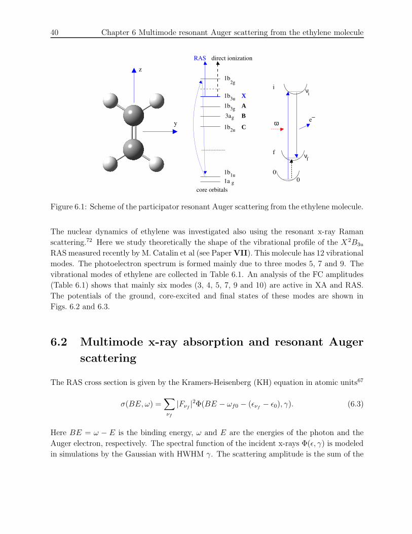
40 Chapter 6 Multimode resonant Auger scattering from the ethylene molecule
3ag
1b2g
1b3u1b3g
1b2u
1b1u1a g
...................
A
B
C
X
core orbitals
RAS direct ionization
e−
νf
νi
00
f
i
ωy
z
Figure 6.1: Scheme of the participator resonant Auger scattering from the ethylene molecule.
The nuclear dynamics of ethylene was investigated also using the resonant x-ray Raman
scattering.72 Here we study theoretically the shape of the vibrational profile of the X2B3u
RAS measured recently by M. Catalin et al (see Paper VII). This molecule has 12 vibrational
modes. The photoelectron spectrum is formed mainly due to three modes 5, 7 and 9. The
vibrational modes of ethylene are collected in Table 6.1. An analysis of the FC amplitudes
(Table 6.1) shows that mainly six modes (3, 4, 5, 7, 9 and 10) are active in XA and RAS.
The potentials of the ground, core-excited and final states of these modes are shown in
Figs. 6.2 and 6.3.
6.2 Multimode x-ray absorption and resonant Auger
scattering
The RAS cross section is given by the Kramers-Heisenberg (KH) equation in atomic units67
σ(BE, ω) =∑
νf
|Fνf|2Φ(BE − ωf0 − (ενf
− ε0), γ). (6.3)
Here BE = ω − E is the binding energy, ω and E are the energies of the photon and the
Auger electron, respectively. The spectral function of the incident x-rays Φ(ε, γ) is modeled
in simulations by the Gaussian with HWHM γ. The scattering amplitude is the sum of the

6.2 Multimode x-ray absorption and resonant Auger scattering 41
Figure 6.2: The ground (g), core-excited (c), and final (f) state potentials of the in-plane
modes 3, 4, 5 and 7 (Table 6.1). We use mass weighted normal coordinates in a.u..
Figure 6.3: Potential energy curves of the torsional modes 9 and 10 (Table 6.1). We use the
same notations as in Fig. 6.2.
direct and the resonant contributions (Fig. 6.1)
Fνf= AD〈νf |0〉 + AR
∑
νi
〈νf |νi〉〈νi|0〉E − ωif − (ενi
− εf ) + ıΓ. (6.4)

42 Chapter 6 Multimode resonant Auger scattering from the ethylene molecule
Table 6.1: Vibrational modes of ethylene. The numbers in brackets show frequencies of the
0-2 transition in core-excited state and the related FC amplitudes of core excitation. The
stars mark the most active modes in x-ray absorption. The potentials of modes 9 and 10
shown here are not modified.mode sym ground(eV) core-exc(eV) FC amplitude 0-1(0-2)
3∗∗ Ag 0.3939 0.4391 0.492
5∗∗ Ag 0.2211 0.2167 -0.484
7∗∗ Ag 0.1799 0.1825 -0.415
4∗∗ B1u 0.3916 0.3952 -0.389
6 B1u 0.1996 0.2086 (0.4173) -0.097 (-0.036)
1 B2u 0.4031 0.4041 0
12 B2u 0.1170 0.1396 0 (0.070)
2 B1g 0.3998 0.4009 0
8 B1g 0.1673 0.1735(0.3475) 0 (-0.026)
11 B3u 0.1400 0.0919 (0.1915) 0 (-0.113)
10∗ B2g 0.1401 0.0731 (0.1594) 0 (-0.184)
9∗ Au 0.1446 0.0630 (0.1373) 0 (0.255)
Usually the direct photoionization is rather weak. Due to this our simulations are performed
taking into account only the resonant scattering channel. We use the following notations:
ωij = Ei − Ej is the spacing between bottoms of the potential surfaces of the electronic
states i and j; ενiis the νith (νi=0, 1, 2, · · · ) vibrational level of the electronic state i,
νi = νiα = νi1, νi2, · · ·νiM, where νiα is the vibrational quantum number of the αth
mode and M = 12 is the total number of vibrational modes. This means that each Franck-
Condon (FC) amplitude 〈νf |νi〉 is the product of the FC amplitudes of all modes∏α
〈νfα|νiα〉.Thus
∑
νi
→M∑
α=1
∑
νiα
, ενi→∑
α
ενiα, 〈νf |νi〉 =
∏
α
〈νfα|νiα〉. (6.5)
Within the Born-Oppenheimer (BO) approximation the amplitude of the direct ionization
is proportional to the scalar product of the polarization vector and the electronic transition
dipole moment of the ionization AD ∝ (e ·d0f), while the amplitude of the resonant channel
is proportional to the amplitudes of photoabsorption and Auger decay AR ∝ (e · d0i)Qif .
The RAS profile (6.3) is obtained using the FC amplitude calculated numerically with the
potentials shown in Figs. 6.2 and 6.3 except for the core-excited state potentials of modes
9 and 10. Following Gadea et al73 we use in simulations more shallow double-minimum
potentials of the core-excited states for modes 9 and 10.

6.2 Multimode x-ray absorption and resonant Auger scattering 43
To understand the formation of the RAS spectral shape we need to know the probability of
excitation of the core-excited vibrational state which is given by the cross section of x-ray
absorption (see Fig. 6.4)
σ(ω) ∝ |di0|2∑
νi
〈νi|0〉2(ω − ωi0 − (ενi
− ε0))2 + Γ2. (6.6)
We use in simulations Γ = 0.05 eV74,75 and γ = 0.05 eV. The assignment of the XA profile
is given in Paper VII.
Figure 6.4: X-ray absorption spectrum versus detuning Ω = ω−ωA of the photon frequency
relative to peak A. Modified modes 9 and 10 for the core-excited states (Paper VII). The
experimental XA spectrum73 (crosses) is shifted to match the theoretical profile.
The theoretical RAS spectra (Fig. 6.5) for different excitation energies are in good agreement
with the experimental data (Fig. 6.6). An assignment of the main RAS features can be found
in Paper VII. Both experiment and theory show spectral features that follow both Raman
and non-Raman dispersions. The origin of these two qualitatively different spectral bands
is two different scattering channels. The fast scattering channel (so-called vertical channel)
has the Raman dispersion law while the non-Raman band is related to the slow resonant
scattering channel.76 The resonant Auger spectra show much stronger vibrational heating
of the ethylene in comparison with the photoelectron spectrum.69,70 The reason for this is
the multimode core excitation (Fig. 6.4).

44 Chapter 6 Multimode resonant Auger scattering from the ethylene molecule
2.0 1.5 1.0 0.5 0.0 -0.5
A
I II
T3
D2
R
Binding Energy (eV)
L
B3
T1
T4
T2
D1
D3
D4
B1
C2
RA
S (
arb.
uni
ts)
C1
B2
R1
Figure 6.5: RAS spectrum of C2H4. The exci-
tation energies and labels correspond to those
in Fig. 6.4. Calculations are performed taking
into account six modes (3, 4, 5, 7, 9, 10) with
five numbers of vibrational levels for each mode.
2.0 1.5 1.0 0.5 0.0 -0.5
Binding Energy (eV)
Left -0.12eV
C 0.4eV
D 0.58eV
RA
S (
arb.
uni
ts)
Top 0.211eV
A Ω=ω−ωA=0
B 0.12eV
Right 0.9eV
Figure 6.6: Experimental resonant Auger spec-
trum of the X2B3u final state of C2H4 for differ-
ent excitation energies.

Chapter 7
Resonant Auger scattering from the
SF6 molecule: Doppler splitting in
circularly polarized x-ray field
Quite often both the core-excited and final states in the RAS process are dissociative ones.
The dissociative atom can reach the region of dissociation during the lifetime of the core-
excited state which is long enough in soft x-ray region (Γ−1 ∼ 10 fs). The Auger decay
in the fragment of dissociation forms a narrow so-called “atomic” peak.77 As predicted in
1998,78 the “atomic” peak experiences electronic Doppler shift
p · v = pv cos θ, (7.1)
which is about 1.0 eV because of the large momentum p of the Auger electron and the high
kinetic energy release ε under dissociation. Here v is the speed of the dissociating atom and
θ = 6 (p,v). The first experimental evidence of this phenomenon was performed in 2000 for
oxygen molecules79 shined by linearly polarized x-rays. Linear polarization was also used in
studies of this effect for other molecules such as ozone80 and SF6.81 Nowadays the Auger
Doppler effect becomes one of the powerful tools in investigation of dissociative states.67
To give insight into the physical mechanism of the Doppler splitting, let us consider the
RAS of the SF6 molecule when the photon frequency ω is tuned near the 1s(F ) → σ∗ x-ray
absorption resonance82 (Fig. 7.1)
ω + SF6 → SF6(1s−1σ∗) → SF5 + F (1s−12p6) → SF5 + F+(2p4) + e−. (7.2)
This is participator RAS. Both v and the transition dipole moment d1s→σ∗ are oriented along
the direction n (|n| = 1) of the S-F∗ bond. The RAS cross section of fixed-in-space molecule

46Chapter 7 Resonant Auger scattering from the SF6 molecule: Doppler splitting in
circularly polarized x-ray field
Inte
nsity
[arb
. uni
ts]
690689688687686
Excitation Energy [eV]
Inte
nsity
[arb
. uni
ts]
710700690680Excitation Energy [eV]
SF6
Total Ion Yield
a1g t1u
t2g
Figure 7.1: The F1s x-ray absorption spectrum of SF6 measured in total ion yield mode.
near the atomic resonance is proportional to the absorption probability Λ(n) = |e · n|2 and
the probability of Auger decay
σ(E, ω, n) = Λ(n) |Q(θ)|2 Γ
π[(∆E − pv cos θ)2 + Γ2], (7.3)
where Q(θ) is the amplitude of the Auger decay, ∆E = E − ωcf , E is the energy of the
Auger electron, ωcf = Ec − Ef is the resonant energy of Auger transition which equals to
the difference between the energies of the core-excited and final states of the fluorine atom,
and Γ is the lifetime broadening of the core-excited state. We omit an unessential prefactor
at the right-hand side of this equation. Conventional RAS spectroscopy measures the RAS
cross section averaged over all molecular orientations
σ(E, ω) =
∫dn
4πσ(E, ω, n). (7.4)
7.1 Linear polarization
Equation (7.3) says that mainly molecules with the SF bonds aligned along the polarization
direction e are core-excited when the light is linearly polarized. Hence, the dissociation
occurs along e. The fluorine atoms dissociate in two opposite directions with opposite
Doppler shifts (-pv, pv) as shown schematically in Fig. 7.2.
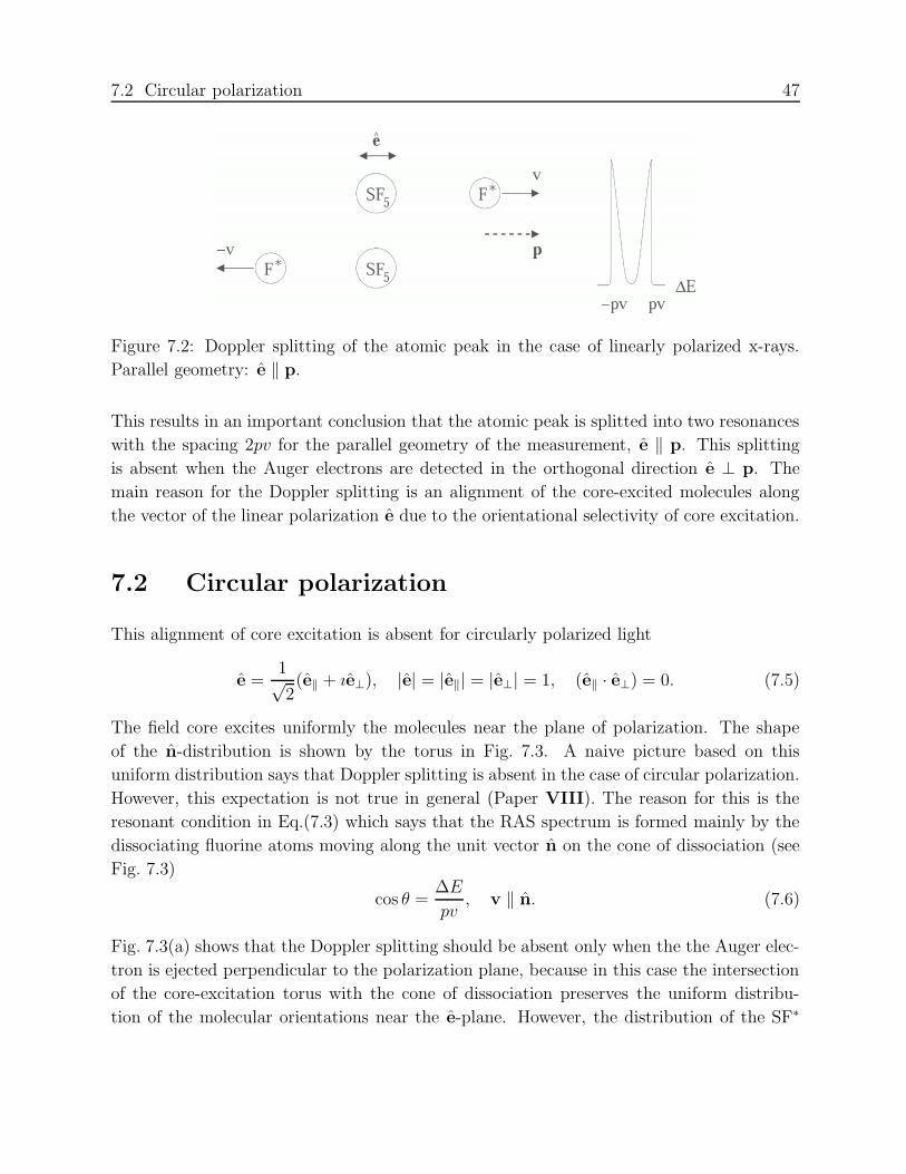
7.2 Circular polarization 47
Figure 7.2: Doppler splitting of the atomic peak in the case of linearly polarized x-rays.
Parallel geometry: e ‖ p.
This results in an important conclusion that the atomic peak is splitted into two resonances
with the spacing 2pv for the parallel geometry of the measurement, e ‖ p. This splitting
is absent when the Auger electrons are detected in the orthogonal direction e ⊥ p. The
main reason for the Doppler splitting is an alignment of the core-excited molecules along
the vector of the linear polarization e due to the orientational selectivity of core excitation.
7.2 Circular polarization
This alignment of core excitation is absent for circularly polarized light
e =1√2
(e‖ + ıe⊥), |e| = |e‖| = |e⊥| = 1, (e‖ · e⊥) = 0. (7.5)
The field core excites uniformly the molecules near the plane of polarization. The shape
of the n-distribution is shown by the torus in Fig. 7.3. A naive picture based on this
uniform distribution says that Doppler splitting is absent in the case of circular polarization.
However, this expectation is not true in general (Paper VIII). The reason for this is the
resonant condition in Eq.(7.3) which says that the RAS spectrum is formed mainly by the
dissociating fluorine atoms moving along the unit vector n on the cone of dissociation (see
Fig. 7.3)
cos θ =∆E
pv, v ‖ n. (7.6)
Fig. 7.3(a) shows that the Doppler splitting should be absent only when the the Auger elec-
tron is ejected perpendicular to the polarization plane, because in this case the intersection
of the core-excitation torus with the cone of dissociation preserves the uniform distribu-
tion of the molecular orientations near the e-plane. However, the distribution of the SF∗

48Chapter 7 Resonant Auger scattering from the SF6 molecule: Doppler splitting in
circularly polarized x-ray field
Figure 7.3: The torus lying in the plane of polarization shows schematically the alignment
of the core-excited molecules by circularly polarized x-rays. The intersection of the torus
with the cone of dissociation (CD) shows the molecules which are active in the RAS.(a)
p ⊥ (e‖, e⊥): No Doppler splitting. (b) p ⊂ (e‖, e⊥): Doppler splitting. (c) The SF∗ bonds
are lying in the polarization plane. No Doppler splitting.
bonds on the cone of dissociation ceases to be uniform in the case of the in-plane geometry
p ⊂ (e‖, e⊥) (Fig. 7.3(b)) and the Doppler splitting can be expected because of the prefer-
ential dissociation in the forward and backward directions relative to p. We would like to
point out that the picture based on Fig. 7.3(b) is not a whole story. When the SF∗ bonds are
lying in the polarization plane (Fig. 7.3(c)), the Doppler splitting is absent in the 2D case,
which contradicts the first impression that the Doppler splitting should be the strongest in
this case. The tilting of the dissociation direction from the plane of polarization plays a
crucial role for the formation of the Doppler splitting.
To describe the Doppler effect we need to know the absorption probability by molecules
with the SF∗ bonds lying on the cone of dissociation (7.6)83
Λ(n) = |e · n|2 =1
2
[(1 − (n · p)2) + (3(n · p)2 − 1)|e · p|2
]. (7.7)
7.2.1 Excitation function for p ⊥ (e‖, e⊥)
Equation (7.7) says that the excitation function
|e · n|2 =1
2sin2 θ, p ⊥ (e‖, e⊥), θ = 6 (p, n) (7.8)
has not peaks at θ = 0, π when the Auger electron is ejected in the direction perpendicular
to the polarization plane (Fig. 7.4(a)). Therefore, the Doppler splitting is absent for the

7.2 Circular polarization 49
circularly polarized light when p ⊥ (e‖, e⊥).
Figure 7.4: (a) Auger electron is
ejected perpendicular to the polariza-
tion plane (e‖, e⊥). (b) Auger elec-
tron is ejected in the polarization plane
(e‖, e⊥). Projection of the direction
of the dissociation n on the plane of
circular polarization (e‖, e⊥). (c) The
excitation is isotropic when n is in
the (e‖, e⊥) plane. (d) The excitation
function is the same as in the case of
linear polarization when n is lying in
the plane orthogonal to e⊥ (ϕ = 900).
7.2.2 Excitation function for p ⊂ (e‖, e⊥)
The picture changes qualitatively when the momentum of the Auger electron is not orthog-
onal to the polarization plane. We will show below that the Doppler splitting exists even
for circularly polarized x-rays by considering the case when p is lying in the polarization
plane. The probability of core excitation of the molecules with the SF bonds oriented along
the cone of dissociation reads
Λ(θ, ϕ) = Λ(n) = |e · n|2 =1
2[(e‖ · n)2 + (e⊥ · n)2] =
1
2(n2
‖ + n2⊥). (7.9)
Providing that e‖ is lying along p (Fig. 7.4(b)), the parallel and the perpendicular compo-
nents of the circular polarization give different contributions in the RAS process
n2‖ = cos2 θ, n2
⊥ = sin2 θ cos2 ϕ. (7.10)
And a surprising result one can see from Eq.(7.10) is that the sum of these two contributions
is anisotropic
Λ(θ, ϕ) =1
2[cos2 θ + sin2 θ cos2 ϕ] =
1
2[1 − sin2 θ sin2 ϕ]. (7.11)

50Chapter 7 Resonant Auger scattering from the SF6 molecule: Doppler splitting in
circularly polarized x-ray field
The excitation is isotropic (no Doppler splitting) only when the direction of dissociation is
lying in the polarization plane (Fig. 7.4(c))
Λ(θ, 0) =1
2, ϕ = 0. (7.12)
The Doppler splitting is absent in this case although there is a large probability n2‖ = cos2 θ
of interaction with e‖. The anisotropy of the excitation is the largest and coincides with the
anisotropy for the linear polarization (Doppler splitting) when the dissociation direction is
lying in the orthogonal plane (ϕ = π/2)
Λ(θ,π
2) =
1
2cos2 θ, ϕ =
π
2. (7.13)
The orthogonal component e⊥ “does not excite” the molecule in this case (Fig. 7.4(d)). The
above two limiting cases (7.12) and (7.13) explain the reason for the Doppler splitting in
the field of circularly polarized light. Indeed, the averaging over ϕ (cos2 ϕ=1/2) gives an
intermediate results between these two cases
Λ(θ) = Λ(θ, ϕ) =1
4[1 + cos2 θ]. (7.14)
The RAS cross section (7.4) in the limit Γ pv
σ(E, ω) =1
2
π∫
0
dθ sin θΛ(θ)|Q(θ)|2δ(∆E − pv cos θ) (7.15)
=|Q(∆E/pv)|2
8pv
1 + (∆E/pv)2 , |∆E| ≤ pv
0, |∆E| ≥ pv
shows the Doppler splitting of the atomic peak with a deep in the resonance ∆E = 0.
Conventionally, the excitation function Λ(θ) can be written through the anisotropy param-
eter β as follows,
Λ(θ) =1
3[1 + βP2(p · n)P2(|p · e|)] =
1
3
1 + βP2(p · n), e ‖ p,
1 − β
2P2(p · n), e ⊥ p,
1 +β
4P2(p · n), circular.
(7.16)
Here P2(x) is the Legendre polynomial. The two upper cases in Eq.(7.16) correspond to the
linear polarization, and one can easily get Eq.(7.14) with β = 2.
7.2 Circular polarization 51
7.2.3 Anisotropy of dissociation and Auger decay
In fact the anisotropy parameter β is smaller than 2. The reason for this is that the velocity
v of the F∗ fragment is not necessarily parallel to the molecular symmetrical axis n (for
example due to the bending vibrations of the dissociating fluorine atom)84
β ≈ 2 − 3〈sin2 δ〉 = 2P2(√
〈cos2 δ〉). (7.17)
Here 〈cos2 δ〉 is the expectation value of cos2 δ with the angle δ = 6 v, n. To get this
expression for β we need to average (p · n)2 over rotations of n around v with a fixed angle
δ:
(p · n)2 =1
2[(1 − (n · v)2) + (3(n · v)2 − 1)(p · v)2] = cos2 θ − P2(cos θ) sin2 δ.
Due to the anisotropy of the molecular orbitals involved in the Auger process, the probability
of Auger decay is not isotropic and depends on the angle θ
|Q|2 ≈ 1 + χP2(p · n). (7.18)
7.2.4 Theoretical and experimental RAS spectra
We calculated the RAS profiles (Fig. 7.5) using parameters from Ref.81 β ≈ 1.4, χ ≈ 0.4, ε =
3.8 eV, and mF = 34618 a.u., µ = 30115 a.u. for ω = 688.3 eV. The velocity of the F atom v
was calculated through the kinetic energy release ε using equation ε = m2Fv
2/(2µ). As shown
in Fig. 7.5, the experiment confirms the theoretical prediction that the circularly polarized
light results in the Doppler splitting and the cross section for the circular polarization equals
to the half sum of the cross sections for the linear polarization with p ‖ e and p ⊥ e
σ(E, ω) =1
2[σ‖(E, ω) + σ⊥(E, ω)], (7.19)
which is in agreement with Eq.(7.16).

52Chapter 7 Resonant Auger scattering from the SF6 molecule: Doppler splitting in
circularly polarized x-ray field
-30369
12
0369
12
654.5 655.0 655.5 656.0 656.5 657.0 657.5 658.00369
12
RAS
cros
s sec
tion
(arb
. uni
ts)
L||
L⊥
E (eV)
C
Figure 7.5: Doppler splitting of the atomic peak of the SF6 molecule. C: circular polarization
(σ(E, ω)). L‖: parallel geometry e ‖ p for linear polarization (σ‖(E, ω)/2); L⊥: perpendic-
ular geometry e ⊥ p for linear polarization (σ⊥(E, ω)/2). β = 1.4, χ = 0.4. Γ = 0.1 eV.
Circles show the experimental data. The theoretical simulations are drawn by solid lines.

Chapter 8
Spontaneous resonant x-ray Raman
scattering induced by core-hole
hopping in strong infrared laser fields
In this chapter, we consider a nonlinear process in the x-ray region, namely resonant inelastic
x-ray Raman scattering (RIXS) in strong laser fields, which provides an opportunity to probe
the dynamics of Rabi flopping of core holes induced by strong laser fields. In many systems,
the core shell consists of few or many close-lying core levels. The molecular orbital splitting
of the core shell lying in the far-IR region (∼ 0.1 eV) is comparable with the lifetime
broadening Γ of the core-excited states. This makes the spectroscopy of core levels rather
difficult to perform. However RIXS associated with the dipole selection rules provides
a direct way to detect the symmetry of the core-excited states,67,85–87 which cannot be
achieved by either nonresonant or nonradiative x-ray spectroscopy.
8.1 Scheme of x-ray–infrared pump-probe spectroscopy
We consider the interaction of diatomic homonuclear molecules with the strong IR laser field
(L), the incident (X1) and the scattered (X2) x-ray fields: Eα(t) = eαEα(t) cos(ωαt + ϕα),
α = L,X1, X2. The effect studied is demonstrated for nitrogen molecules with the splitting
of the gerade and ungerade core levels88 ∆ =0.097 eV lying in the far-IR region (λ ≈12.8µm).
The RIXS of N2 with the ground-stateX1Σ+g [ψ0 = |(1σg)2, (1σu)2, (2σg)2, (2σu)2, (1πu)4, (3σg)2〉]
was studied experimentally earlier.67,87 The RIXS spectra show only a single resonant tran-

54Chapter 8 Spontaneous resonant x-ray Raman scattering induced by core-hole hopping in
strong infrared laser fields
3σ−1g 1π 1
g Π1g
( )
2σ−1u 1π 1
g Π1u
( )
1π 1g1π −1
u
1σ−1u 1π 1
g Π1u
)(
∆ u1
Σ u1 −
Σ u1 +
Σ g1 +
1σ−1g Π1
g1π 1g
)(
final states
core−excited states
1:
2:
f:
0: ground state
X1
X2
IR field
Figure 8.1: Scheme of resonant x-ray Raman scattering from the N2 molecule in a IR field.
Dashed lines show the dipole forbidden transitions. Taken from Paper IX. Reprinted with
permission of American Physical Society.
sition 3σg → 1σu when the x-ray photon frequency ωX1 is tuned in resonance with the lowest
unoccupied molecular orbital (LUMO) 1πg. The reason for this is that the incident x-ray
photon creates only an ungerade core hole in 1σu. The gerade core level is not involved
in RIXS because the absorption transition 1σg → 1πg is forbidden (Fig. 8.1). The picture
changes qualitatively when the core-excited molecule is illuminated by IR radiation tuned
near the resonance between 1σg and 1σu core levels. The IR field transfers the ungerade core
hole to the gerade core level 1σu → 1σg. Due to this, the symmetry forbidden transitions
from ungerade MOs (1πu, 2σu) are now allowed and the RIXS spectrum changes drastically.
8.2 Amplitude equations and RIXS cross sections
The x-ray and the IR fields mix the ground (ψ0), the two core-excited (ψ1 ≡ |1σ−1u 1π1
g〉,ψ2 ≡ |1σ−1
g 1π1g〉) and the five final states (ψf ) (Fig. 8.1): ψ =
∑aiψi. When the weak
incident x-ray field does not change the ground-state population, a0 ≈ 1, and the weak
scattered spontaneous x-ray field does not affect the population of the core-excited states,
both of the weak x-ray fields can be treated within RWA, while the strong IR-laser field
should be taken into account explicitly. Under the above conditions, the dynamics of the

8.2 Amplitude equations and RIXS cross sections 55
population of the core-excited states obey the amplitude equations
a1 + Γa1 =ı
2e−ıΩX1tGX1
10 a0 + ıe−ıω21tGL12 cos(ωLt)a2,
a2 + Γa2 = ıeıω21t cos(ωLt)GL21a1, GX1
20 = 0. (8.1)
The pump field populates only the core-excited state ψ1, because the transition ψ0 → ψ2 is
dipole forbidden. The final state is populated due to the spontaneous decays (field X2)
af + Γfaf =ı
2
[eıΩ
(1)X2tGX2
f1 a1 + eıΩ(2)X2tGX2
f2 a2
]. (8.2)
Here Γ and Γf are the lifetime broadenings of the core-excited and final states, respectively,
and the detunings ΩX1 = ωX1 − ω10, Ω(n)X2 = ωX2 − ωnf , n = 1, 2. Gα
ij = (eα · dij)Eα/h
are Rabi frequencies of the x-ray transitions (α = X1, X2) and the IR transitions between
the core-excited states (α = L). When the laser field EL is strong enough (|GL12| > Γ), the
molecule oscillates between the core-excited states 1 and 2 at the Rabi frequency GL21.
The RIXS cross section σ =∑f
σf is computed through the integral of the final-state pop-
ulation (ρf (t) = |af(t)|2):
σf ∝∫ ∞
−∞
ρf (t)dt. (8.3)
The RIXS depends on the orientations of the polarization vectors of the x-ray fields and
IR-laser field relative to the transition dipole moments through the Rabi frequencies. It is
easy to extract the polarization factors related to the x-ray fields. This allows us to write
down the RIXS cross section for fixed-in-space molecules as
σ(θ) = sin2 θX1[cos2 θX2
σ3σg
(θ) + σ2σu(θ)
(8.4)
+1
2sin2 θX2
(σ
1Σ−
u
1πu(θ) + σ
1Σ+u
1πu(θ) + 2σ
1∆u
1πu(θ))
].
Here θX1 = 6 eX1,R, θX2 = 6 eX2,R and θ = 6 eL,R are the angles between the polarization
vectors of the x-ray and IR fields and the molecular axis R. The partial RIXS cross sections
σf(θ) at the right-hand side of Eq.(8.4) depend only on the orientation of the IR field relative
to R: θ = 6 eL,R. These partial cross sections (8.3) are computed using the solution of the
amplitude Eqs.(8.1) and (8.2) for eX1 ‖ d10 and eX2 ‖ dfc.
From Eq.(8.4) one can see that the RIXS cross section depends on the relative polarization
direction of the fields. We consider here two geometries of the RIXS (see Paper IX).
• Geometry A The polarizations of the incident laser pulse and of the emitted x-ray
radiation are parallel to each other and they are perpendicular to that of the incident
x-ray pulse: (eL ‖ eX2) ⊥ eX1, θ = θX2.

56Chapter 8 Spontaneous resonant x-ray Raman scattering induced by core-hole hopping in
strong infrared laser fields
• Geometry B The polarizations of the two x-ray fields are parallel to each other and
they are perpendicular to that of the IR-laser pulse: eL ⊥ (eX2 ‖ eX1), θX1 = θX2.
Usually measurements are performed for gas phase molecules. Due to this our simulations
are performed for randomly oriented molecules with orientational averaging.
8.3 Opening of symmetry-forbidden RIXS channels
The effect studied here depends on the competition of the time of Rabi flopping between the
core holes τR, the duration of the x-ray pulse τX1, and the duration of the scattering τRIXS .
The time of Rabi flopping τR = π/GL21 determines the efficiency of the core hole hopping
between the ungerade and gerade core levels. Fig. 8.2 shows the RIXS spectra calculated
from Eqs.(8.1) for geometry A as functions of the intensity of the IR field. One can see that
when the IR-laser pulse is weak, only the symmetry allowed channel is observed. However,
when the intensity of the IR pulse is strong enough [IL > Ith = 2cε0(hΓ/d12)2 ≈ 1012
W/cm2] to make the Rabi frequency of the IR transition comparable or larger than the
Figure 8.2: Partial RIXS cross sections versus the peak intensity IL of the IR field for
Geometry A. The HWHM of the pulses τX = τL = 1 ps. ΩX1 = ΩL = 0. ϕX1 = ϕL = 0.
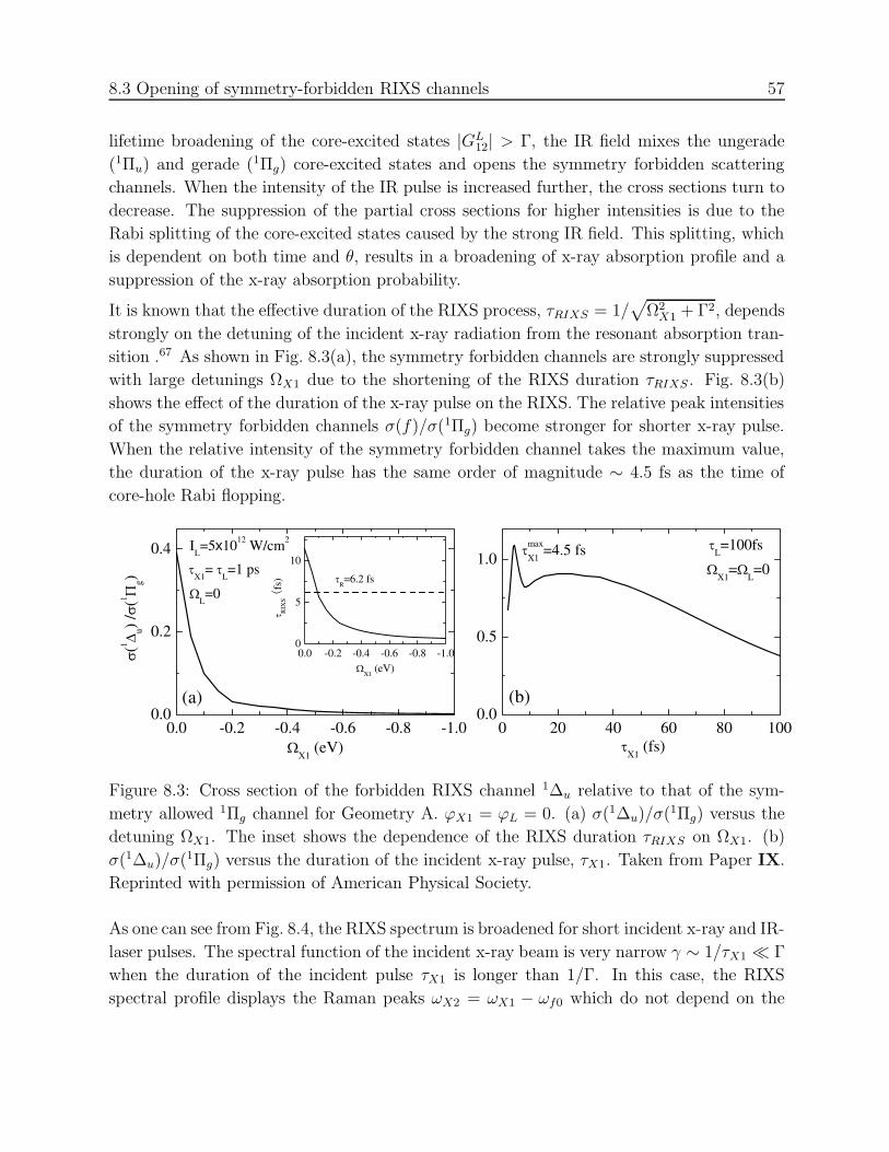
8.3 Opening of symmetry-forbidden RIXS channels 57
lifetime broadening of the core-excited states |GL12| > Γ, the IR field mixes the ungerade
(1Πu) and gerade (1Πg) core-excited states and opens the symmetry forbidden scattering
channels. When the intensity of the IR pulse is increased further, the cross sections turn to
decrease. The suppression of the partial cross sections for higher intensities is due to the
Rabi splitting of the core-excited states caused by the strong IR field. This splitting, which
is dependent on both time and θ, results in a broadening of x-ray absorption profile and a
suppression of the x-ray absorption probability.
It is known that the effective duration of the RIXS process, τRIXS = 1/√
Ω2X1 + Γ2, depends
strongly on the detuning of the incident x-ray radiation from the resonant absorption tran-
sition .67 As shown in Fig. 8.3(a), the symmetry forbidden channels are strongly suppressed
with large detunings ΩX1 due to the shortening of the RIXS duration τRIXS . Fig. 8.3(b)
shows the effect of the duration of the x-ray pulse on the RIXS. The relative peak intensities
of the symmetry forbidden channels σ(f)/σ(1Πg) become stronger for shorter x-ray pulse.
When the relative intensity of the symmetry forbidden channel takes the maximum value,
the duration of the x-ray pulse has the same order of magnitude ∼ 4.5 fs as the time of
core-hole Rabi flopping.
0.0 -0.2 -0.4 -0.6 -0.8 -1.00
5
10
0.0 -0.2 -0.4 -0.6 -0.8 -1.00.0
0.2
0.4
RIX
Sfs
)
X1 (eV)
R=6.2 fs
0 20 40 60 80 1000.0
0.5
1.0
(b)
maxX1 =4.5 fs
X1 (fs)
L=100fs
X1= L=0
L=0X1= L=1 ps
IL=5x10¹² W/cm2
(a)
(u) /
(g)
X1 (eV)
Figure 8.3: Cross section of the forbidden RIXS channel 1∆u relative to that of the sym-
metry allowed 1Πg channel for Geometry A. ϕX1 = ϕL = 0. (a) σ(1∆u)/σ(1Πg) versus the
detuning ΩX1. The inset shows the dependence of the RIXS duration τRIXS on ΩX1. (b)
σ(1∆u)/σ(1Πg) versus the duration of the incident x-ray pulse, τX1. Taken from Paper IX.
Reprinted with permission of American Physical Society.
As one can see from Fig. 8.4, the RIXS spectrum is broadened for short incident x-ray and IR-
laser pulses. The spectral function of the incident x-ray beam is very narrow γ ∼ 1/τX1 Γ
when the duration of the incident pulse τX1 is longer than 1/Γ. In this case, the RIXS
spectral profile displays the Raman peaks ωX2 = ωX1 − ωf0 which do not depend on the

58Chapter 8 Spontaneous resonant x-ray Raman scattering induced by core-hole hopping in
strong infrared laser fields
energies of the core-excited states (Fig. 8.2). The picture changes qualitatively when the
x-ray pulse is short γ ∼ 1/τX1 ≥ Γ. Now both Raman (ωX2 = ωX1 − ωf0) and non-Raman
(ωX2 = ωcf) peaks are seen in RIXS. The appearance of the extra peaks in the RIXS profile
shown in Fig. 8.4 (a) is caused by the Rabi splitting of the core-excited states.
It is natural to expect a phase sensitivity of the RIXS when the pulses are short. To check
the role of the CEP, we calculated the RIXS profiles for different phases of short x-ray and
IR pulses. Simulations shown in Fig. 8.4 (b) display the phase sensitivity of the RIXS. We
calculated also the spectra for another two different sets of phases (ϕX1 = 0, ϕL = π/2) and
(ϕX1 = π/4, ϕL = π/2) with the same phase of the IR field. These two sets of phases give
exactly the same profiles. This means that the RIXS profile is sensitive only to the absolute
phase ϕL of the few-cycle strong IR field and does not depend on the phase of the weak
x-ray pulse ϕX1.
386 387 388 389 390 391 392 3930
1
2
0.0
0.5
1.0
L= X1=
L= /2, X1=
L= X1=3.5fs
L= X1=
(b)
L=100fs X1=2.75fs
X2 (eV)
(arb
. uni
ts)
(a)
Figure 8.4: (a) RIXS spectra for short incident X-ray and IR-laser pulses with Geometry
A. (b) Phase effect on RIXS of short pulses. IL = 5.0 × 10¹² W/cm2. Taken from Paper
IX. Reprinted with permission of American Physical Society.

Chapter 9
Role of stimulated resonant x-ray
Raman scattering on Auger effect
Auger effect is one of the important spectroscopic tools in molecular and material science.
Nevertheless, the Auger effect becomes undesirable when the strong XFEL pulse propagates
through the resonant medium because the Auger decay is the main channel of ionization
during the propagation of the x-ray pulse. The Auger ionization followed by the Coulomb
explosion becomes the major reason of radiative damage. In this chapter, we study the effects
of propagation of strong XFEL pulses on the relative Auger rate by solving numerically
the coupled Maxwell’s (3.9) and density matrix equations (2.24), and find out the way to
suppress Auger decay during pulse propagation (Paper X).
9.1 Basic physics: Auger branching ratio
We select for our study the gas phase argon atom described by a three-level scheme shown in
Fig. 9.1. The strong x-ray field tuned in resonance with the 2p3/2 → 4s transition couples the
core-excited state (|1〉 = |2p−13/2〉) with the ground state (|0〉, ω10 = 244.3 eV,89 d10 = 0.0204
a.u.) and the Stokes state (|2〉 = |3s−14s〉, ω12 = 219.28 eV,90 d12 = 0.048 a.u.). To analyze
the role of the XFEL field on the Auger effect it is enough to analyze the population of the
core-excited state ρ11 and the total population
∂
∂tρ11 = −Γρ11 +W = − (Γρ11 +WE) +WA, (9.1)
∂
∂tρ = −Γρ11 − Γfρ22, ρ = ρ00 + ρ11 + ρ22.

60 Chapter 9 Role of stimulated resonant x-ray Raman scattering on Auger effect
Here the small lifetime broadenings caused by spontaneous decays are neglected, and the
Auger decay rates of the core-excited and final states are Γ = 0.12 eV89 and Γf = 0.076
eV,91 respectively. The probability of radiative population or depopulation of the core-
excited state induced by the XFEL pulse is depicted by the field work W (z, t),
W (z, t) = 2=∑
n=0,2
(V1n(z, t)ρn1(z, t)eıω1nt
), Vnm(z, t) = −E(z, t)dnm/h. (9.2)
Fig. 9.2 gives the temporal distribution of the field work W (z, t) induced by gaussian pulses
(Eq.(4.7), m = 1). W (z, t) shows a sign-changing property which is determined by the pulse
area and the instantaneous Rabi frequency. Therefore, it is convenient to divide W (z, t) into
positive WA(z, t) > 0 and negative −WE(z, t) < 0 parts which represent respectively the
absorption and the stimulated emission induced by the incident XFEL pulse.
Figure 9.1: Scheme of transitions in Argon atom: resonant (0-1) and Stokes (1-2) channels.
|1〉 = |2p−13/24s〉, |2〉 = |3s−14s〉.
One can see from the rate equation (9.1) of ρ11(z, t) that the core-excited state is populated
with the rate of WA(z, t) and is depopulated with the rate of Γρ11(z, t) + WE(z, t) due to
Auger decay and the stimulated emission. Therefore, the instantaneous branching ratio of
the Auger decay can be defined as w(z, t) = Γρ11(z, t)/(Γρ11(z, t) +WE(z, t)). Usually time
statistical measurement is performed in real experiment, so we introduce the time integral
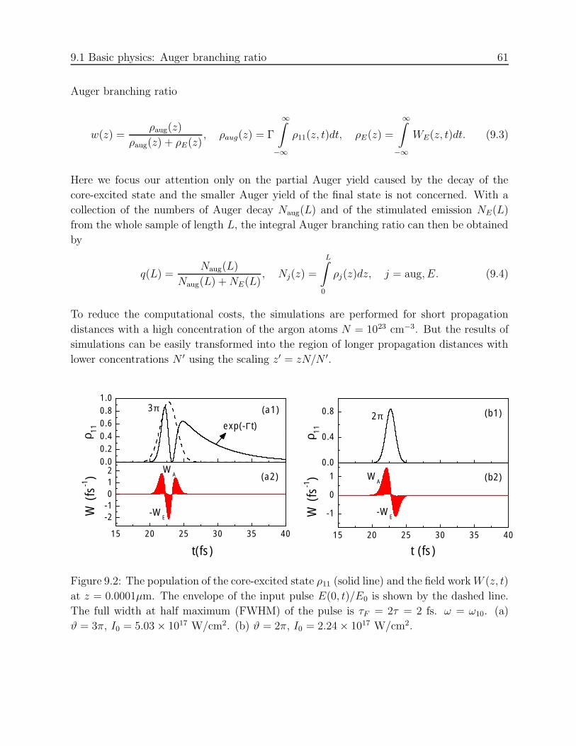
9.1 Basic physics: Auger branching ratio 61
Auger branching ratio
w(z) =ρaug(z)
ρaug(z) + ρE(z), ρaug(z) = Γ
∞∫
−∞
ρ11(z, t)dt, ρE(z) =
∞∫
−∞
WE(z, t)dt. (9.3)
Here we focus our attention only on the partial Auger yield caused by the decay of the
core-excited state and the smaller Auger yield of the final state is not concerned. With a
collection of the numbers of Auger decay Naug(L) and of the stimulated emission NE(L)
from the whole sample of length L, the integral Auger branching ratio can then be obtained
by
q(L) =Naug(L)
Naug(L) +NE(L), Nj(z) =
L∫
0
ρj(z)dz, j = aug, E. (9.4)
To reduce the computational costs, the simulations are performed for short propagation
distances with a high concentration of the argon atoms N = 1023 cm−3. But the results of
simulations can be easily transformed into the region of longer propagation distances with
lower concentrations N ′ using the scaling z′ = zN/N ′.
15 20 25 30 35 40
-2-1012
-WE
(a2)
t(fs)
W (
fs-1) W
A
0.00.20.40.60.81.0
ρ 11 exp(-Γt)
(a1)3π
15 20 25 30 35 40
-1
0
1
-WE
WA (b2)
W (
fs-1)
t (fs)
0.0
0.4
0.8 2π (b1)
ρ 11
Figure 9.2: The population of the core-excited state ρ11 (solid line) and the field work W (z, t)
at z = 0.0001µm. The envelope of the input pulse E(0, t)/E0 is shown by the dashed line.
The full width at half maximum (FWHM) of the pulse is τF = 2τ = 2 fs. ω = ω10. (a)
ϑ = 3π, I0 = 5.03 × 10¹⁷ W/cm2. (b) ϑ = 2π, I0 = 2.24 × 10¹⁷ W/cm2.

62 Chapter 9 Role of stimulated resonant x-ray Raman scattering on Auger effect
9.2 Role of pulse reshaping on Auger branching ratio
The propagation of strong XFEL pulses in the atomic Argon medium is accompanied by
strong nonlinear effects such as pulse compression, ASE, stimulated resonant Raman scat-
tering (SRRS), lasing without inversion (LWI), and FWM. Therefore, the XFEL pulse will
be severely reshaped, which will change remarkably the Auger branching ratio.
20 30 40 50 60 70
-0.4
-0.2
0.0
0.2
0.4
0.6
0.8
1.0
z=0.42µm
W (
fs-1)
t (fs)
z=0
W
(a)
0 1 2 3 4 5 60.0
0.2
0.4
0.6
0.8
1.0
z(µm)
Aug
er y
ield
zC
q
aug
(b)
Figure 9.3: ϑ = π, I0 = 5.59 × 10¹⁶ W/cm2. FWHM τF = 2 fs. ω = ω10. (a) The field
work W (z, t) and the envelope E(z, t)/E0 (solid line) at z = 0.42µm with Γ = 0 in the
two-level approximation which considers only the ground and the core-excited states. The
dashed and solid lines show respectively the envelope E(0, t)/E0 of the input pulse and of
the pulse at 0.42µm. (b) The Auger yield ρaug(z) (9.3), the branching ratio w(z) (9.3), and
the integral branching ratio q(L) (9.4) versus the propagation distance in the three-level
Argon medium.

9.2 Role of pulse reshaping on Auger branching ratio 63
9.2.1 Burnham-Chiao oscillations
From Eq.(9.3) one can see that the Auger branching ratio can be suppressed by stimulated
emission induced by the XFEL. As shown in Fig. 5.1(a), McCall-Hahn area theorem (5.1)
says that when a pulse with its area smaller than π propagates in an absorbing medium,
the area of the whole pulse will be decreased gradually and no stimulated emission occurs,
hence, the Auger branching ratio is constant, w = 1. However, it was shown by Burnham
and Chiao92 that during pulse propagation the envelope of the field E(z, t) follows the sine-
Gordon equation and experiences Burnham-Chiao oscillations 92 (see Fig. 9.3 (a)). This
results in a sign-changing temporal shape of the field work (Fig. 9.3 (a)) and reduces the
Auger branching ratio w(z) already for pulses with ϑ ≤ π (Fig. 9.3 (b)).
20 30 40 50 60 70
1
2
3
4
5
6
-1
-0.6
-0.2
0.2
0.6
1
z (µ
m)
t (fs)
(b)
20 30 40 50 60 70
1
2
3
4
5
6
-1
-0.6
-0.2
0.2
0.6
1
t (fs)
z (µ
m)
z(a)
c
Figure 9.4: The 2D maps of the population inversions, which are quenched in the region
z > zc ' 5.5µm. ϑ = 3π, τF = 2 fs. (a) ρ11(z, t) − ρ00(z, t), (b) ρ11(z, t) − ρ22(z, t).
9.2.2 Stimulated resonant Raman scattering
The population distribution (4.1) for a two-level system shows that an external pulse with
the initial area around (2n + 1)π inverts the population ρ11(z, t) − ρ00(z, t) > 0, and the
amplified spontaneous emission started from noise can be expected in the inverted medium.
In the studied three-level system, although the carrier frequency of the strong XFEL is
tuned in resonance with the transition |0〉 → |1〉, and the |1〉 → |2〉 transition is away
from resonance with a large detuning ω − ω12 ' 25 eV, the Burnham-Chiao oscillations
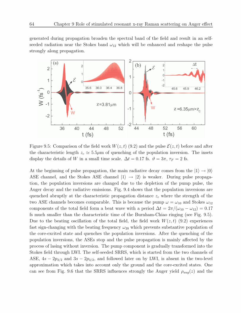
64 Chapter 9 Role of stimulated resonant x-ray Raman scattering on Auger effect
generated during propagation broaden the spectral band of the field and result in an self-
seeded radiation near the Stokes band ω12 which will be enhanced and reshape the pulse
strongly along propagation.
Figure 9.5: Comparison of the field work W (z, t) (9.2) and the pulse E(z, t) before and after
the characteristic length zc ' 5.5µm of quenching of the population inversion. The insets
display the details of W in a small time scale. ∆t = 0.17 fs. ϑ = 3π, τF = 2 fs.
At the beginning of pulse propagation, the main radiative decay comes from the |1〉 → |0〉ASE channel, and the Stokes ASE channel |1〉 → |2〉 is weaker. During pulse propaga-
tion, the population inversions are changed due to the depletion of the pump pulse, the
Auger decay and the radiative emissions. Fig. 9.4 shows that the population inversions are
quenched abruptly at the characteristic propagation distance zc where the strength of the
two ASE channels becomes comparable. This is because the pump ω = ω10 and Stokes ω12
components of the total field form a beat wave with a period ∆t = 2π/(ω10 − ω12) = 0.17
fs much smaller than the characteristic time of the Burnham-Chiao ringing (see Fig. 9.5).
Due to the beating oscillation of the total field, the field work W (z, t) (9.2) experiences
fast sign-changing with the beating frequency ω20 which prevents substantive population of
the core-excited state and quenches the population inversions. After the quenching of the
population inversions, the ASEs stop and the pulse propagation is mainly affected by the
process of lasing without inversion. The pump component is gradually transformed into the
Stokes field through LWI. The self-seeded SRRS, which is started from the two channels of
ASE, 4s − 2p3/2 and 3s − 2p3/2, and followed later on by LWI, is absent in the two-level
approximation which takes into account only the ground and the core-excited states. One
can see from Fig. 9.6 that the SRRS influences strongly the Auger yield ρaug(z) and the

9.3 Effect of direct photoionization 65
Auger branching ratio w(z). ρaug(z) and w(z) drops down very fast in the region near zc
where the population of the core-excited state becomes small.
To conclude, the sign-changing modulation of the field work caused by Burnham-Chiao os-
cillations results in a quasiperiodical following of the absorption by the stimulated emission.
This reduces the population of the core-excited state as well as the Auger yield and branch-
ing ratio. The competition between the Auger decay and the stimulated emission is the main
reason for the suppression of the Auger branching ratio. In the region where the strength
of the pump and Stokes fields becomes comparable, the fast beating oscillation formed by
these two fields quenches abruptly the population inversions and suppresses strongly the
Auger branching ratio. After that, the Stokes lasing occurs without population inversion,
and the Auger branching ratio changes smoothly and slowly due to the small population of
the core-excited state.
0 1 2 3 4 5 6 7 8
0.2
0.4
0.6
0.8
1.0
z(µm)
(b)
0 1 2 3 4 5 6 7 8
0.0
0.2
0.4
0.6
0.8
1.0
Aug
er y
ield
z(µm)
q ρ
aug
(a)
zC
Figure 9.6: Comparison of the Auger yield and Auger branching ratios for three-level (a)
and two-level (b) models. FWHM τF = 2 fs. ϑ = 3π (I0 = 5.03 × 10¹⁷ W/cm2).
9.3 Effect of direct photoionization
The main channels of ionization of the studied system are the Auger decays of the core-
excited and final states with the relaxation rates Γ and Γf . But the strong X-ray radiation
can ionize directly the Ar atoms. Because the photon frequency is below the ionization
threshold of the 2p3/2 electrons, the only ionization channels are the direct ionization of
electrons from outer shells 3s and 3p. According to experimental data93 the corresponding

66 Chapter 9 Role of stimulated resonant x-ray Raman scattering on Auger effect
photoionization cross section is about σph ≈ 0.3 Mb. The direct photionization affects the
Bloch equation due to the additional relaxation of the populations and the off-diagonal
elements of the density matrix (2.24)
Γn → Γn + γ(n)ph (t), γmn → γmn +
1
2(γ
(n)ph (t) + γ
(m)ph (t)) (9.5)
caused by the rate of the direct photoionization of the nth level γ(n)ph (t) = σ
(n)ph I(t)/hω, where
I(t) = |E(t)H(t)| is the instantaneous intensity of the light.
To be consistent with the experimental x-ray absorption cross section93,94 σ10 = 2 Mb of the
2p3/2 → 4s transition, we used the transition dipole moments dexp10 =
√137σ10Γ/(8πω) ≈
6.7 × d10 = 0.137a.u. and dexp12 ≈ d12d
exp10 /d10 ≈ 0.322a.u.. The increase of the transition
dipole moments results in a significant decrease of the peak intensity of the XFEL pulse
Iexp0 = I0 × (d10/d
exp10 )2 ≈ I0/44.89. Fig. 9.7 shows the Auger branching ratios with and
without direct photoionization for a 3π pulse with the FWHM of τF = 2.0 fs. One can see
that the role of the direct photoionization is not significant for the pulse with an intensity
level of 1016 W/cm2. It increases slightly the Auger ratios and does not change very much the
dynamics of Auger decay. The relative number of ionized atoms is also small: ρion/ρ(0) =
1 − e−p ∼ p =∫∞
−∞γph(t)dt ∼ γmax
ph τ√π/ln2 ∼ 10%. The main reason for this is the rather
long photoionization time τph = 1/γmaxph ≈ 11.7 fs in comparison with the time of Auger
decay 1/Γ ≈ 5.5 fs and the pulse duration τF = 2 fs.
0.00 0.05 0.10 0.15 0.20 0.25 0.30
0.1
0.2
0.3
0.4
0.5
0.6 σph=0
q
σph=0.3 Mb q
Aug
er y
ield
z(µm)
Figure 9.7: Comparison of the Auger branching ratios w(z) (9.3) and q(L) (9.4) with and
without direct photoionization. FWHM τF = 2 fs. ϑ = 3π, Iexp0 = 1.1 × 10¹⁶ W/cm2.

Chapter 10
Summary of results
This thesis contains a collection of results obtained during my Ph.D. studies in the fields of
nonlinear optics and x-ray spectroscopy. The following main results have been obtained:
1. Quantum coherent control
• It is shown that the variation of the duration, shape and intensity of the pump pulse
allows a quantum control of the nuclear wave packet, which means the selective pop-
ulation of certain vibrational levels and preparation of the wave packet of desirable
shape.
• A strict analytical solution of two-photon interaction with multilevel molecules has
been found beyond the rotating wave approximation (RWA).
• The major role of the non-RWA corrections is the change of the dynamical Stark shifts.
The standard RWA gives a wrong expression of the dynamical Stark shifts. Complete
breakdown of standard RWA for two-photon absorption process is observed even for
a rather weak field with its Rabi frequency much smaller than the light frequency.
• For fixed-in-space molecules, the compensation of the dynamical Stark effect can be
achieved by detuning and phase tailoring. The orientational disorder diminishes sig-
nificantly the efficiency of the two-photon induced population transfer and does not
allow complete compensation of the dynamical Stark shift. But the polarization sen-
sitivity of the photobleaching resulted from molecular anisotropy can be used for data
storage.
2. Two-photon induced optical limiting
68 Chapter 10 Summary of results
• The ”two-photon area theorem” which describes the evolution of the energy fluence of
a pulse propagating two-photon resonantly in a molecular medium is derived beyond
RWA by taking into account the dynamical Stark shifts and the permanent dipole
moments.
• A dynamical theory of the sequential two-photon absorption of microsecond pulses
involving singlet-singlet and triplet-triplet transitions is developed, and the effect of
the transverse inhomogeneity of the light beam is taken into account.
• The propagation effect plays an important role in the performance of the sequential
two-photon absorption induced optical power limiting because of the competition be-
tween the nonlinear two-step TPA and the linear one-photon absorption which depends
on the field intensity, the length of the absorber and the concentration.
3. Superfluorescence and supercontinuum generation
• It is found that the intensity of the two-color superfluorescence is enhanced by increase
the concentration of the molecules, while the fast dephasing of the dipole coherence
reduces the intensity of the cooperative radiation and delays the emission of superflu-
orescence or even inhibits the formation of the emission.
• An attosecond pulse is formed by pulse splitting when a femtosecond pulse with a
large area propagates resonantly in a two-level molecular medium.
• The supercontinuum generation of the spectrum is mainly caused by the self-phase
modulation of the fore-going subpulse and is sensitive to the initial carrier-envelope
phase of the pulse.
• Strong-field photoionization suppresses the fine structure of the spectrum caused by
the interference between the subpulses and decreases the intensity of the subpulses.
4. Multimode resonant Auger scattering
• Ab-initio simulations of the multimode resonant Auger scattering have been performed
for the ethylene molecule. Results of simulations which show good agreement with
the experimental data explain the main spectral features.
• The RAS spectra show much stronger vibrational heating of the ethylene molecule in
comparison with the photoelectron spectrum due to multimode core excitation.
• Raman and non-Raman dispersions seen in the RAS spectra are attributed respectively
to the fast and slow scattering channels.

69
5. Auger Doppler effect
• The Doppler splitting of the atomic peak in resonant Auger scattering for circularly
polarized x-rays is predicted theoretically and is confirmed experimentally.
• The Doppler splitting is absent when the Auger electron is ejected perpendicular to
the plane of circularly polarized x-rays. The atomic peak is Doppler splitted when the
momentum of the Auger electron is not orthogonal to the polarization plane.
• The Doppler profile for circular polarization equals to one-half of the sum of the
Doppler profiles for parallel and orthogonal orientations of the linearly polarized light.
6. Spontaneous x-ray Raman scattering in strong IR laser fields
• A new scheme of x-ray pump-probe experiment, resonant inelastic x-ray Raman scat-
tering accompanied by core-hole hopping induced by strong laser fields, is suggested.
The theory is exemplified in details for the N2 molecule.
• It is shown that a strong-laser-field induced promotion of the ungerade core hole
created by a weak x-ray pulse to a gerade core level opens up the symmetry forbidden
scattering channels and gives rise to new spectral lines in the x-ray scattering spectrum.
• The symmetry forbidden scattering channel is strongly enhanced when the time of
Rabi flopping becomes shorter than the lifetime of the core-excited state.
7. Stimulated x-ray Raman scattering
• The propagation of a strong XFEL pulse with its frequency below core ionization
threshold is accompanied by self-seeded stimulated resonant x-ray Raman scattering
initiated by the spectral broadening of Burnham-Chiao oscillation.
• The population inversion is quenched abruptly near a critical distance where the pump
and enhanced Stokes fields strongly interfere with each other. After this critical dis-
tance, the region of amplified spontaneous emission is followed by lasing without in-
version, and the Auger yield becomes very weak.
• The Auger yield is strongly suppressed in the course of pulse propagation due to the
stimulated x-ray emissions and the fast oscillation of the field work.

70 Chapter 10 Summary of results

Bibliography
[1] A. C. Newell and J. V. Moloney, Nonlinear Optics, Addsion-Wesley Publishing Com-
pany, 1992.
[2] S. Svanberg, Atomic and Molecular Spectroscopy: Basic Aspects and Practical Appli-
cations, 3rd Edition, Springer, 2001.
[3] A. H. Zewail 2000 J. Phys. Chem. A 104 5660.
[4] C. Bressler and M. Chergui 2004 Chem. Rev. 104 1781.
[5] S. Techert, F. Schotte, and M. Wulff 2001 Phys. Rev. Lett. 86 2030.
[6] R. Neutze, R. Wouts, S. Techert, J. Davidsson, M. Kocsis, A. Kirrander, F. Schotte,
and M. Wulff 2001 Phys. Rev. Lett. 87 195508.
[7] M. Drescher, M. Hentschel, R. Klenberger, M. Ulberacker, V. Yakovlev, A. Scrinzl, Th.
Westerwalbesloh, U. Kleineberg, U. Heinzmann, and F. Krausz 2002 Nature 419 803.
[8] K. Tiedtke, A. Azima, N. von Bargen, L. Bittner, S. Bonfigt, S. Duterer, B. Faatz,
U. Fruling, M. Gensch, Ch. Gerth, N. Guerassimova, U. Hahn, T. Hans, M. Hesse, K.
Honkavaar, U. Jastrow, P. Juranic, S. Kapitzki, B. Keitel, T. Kracht, M. Kuhlmann, W.
B. Li, M. Martins, T. Nunez, E. Plonjes, H. Redlin, E. L. Saldin, E. A. Schneidmiller,
J. R. Schneider, S. Schreiber, N. Stojanovic, F. Tavella, S. Toleikis, R. Treusch, H.
Weigelt, M. Wellhofer, H. Wabnitz, M. V. Yurkov, and J. Feldhaus 2009 New J. Phys.
11 023029.
[9] S. T. Hendow and S. A. Shakir 1986 Appl. Opt. 25 1759.
[10] W. H. Press, S. A. Teukolsky, W. T. Vetterling, and B. P. Flannery Numerical Recipes:
The Art of Scientific Computing, 3rd Edition, Cambridge University Press, 2007.
[11] K. S. Yee 1966 IEEE Trans. Antennas Propag. 14 302.

72 BIBLIOGRAPHY
[12] R. W. Ziolkowski, J. M. Arnold, and D. M. Gobny 1995 Phys. Rev. A 52 3082.
[13] A. V. Tarasishin, V. A. Magnitskii, V. A. Shuvaev, and A. M. Zheltikov 2001 Opt.
Express 8 452.
[14] G. Mur 1981 IEEE Trans. Electromagn. Compat. EMC-23 377.
[15] Z. P. Liao, H. L. Wong, B. P. Yang, and Y. F. Yuan 1984 Scientia Sinica A 27 1063.
[16] J. Berenger 1994 J. Comput. Phys. 114 185.
[17] A. Taflove and S. C. Hagness, Computational Electrodynamics: The Finite-Difference
Time-Domain Method, 3rd edition, Artech House Publishers, 2005.
[18] H. A. Rabitz, M. M. Hsieh, and C. M. Rosenthal 2004 Science 303 1998.
[19] M. P. A. Branderhorst, P. Londero, P. Wasylczyk, C. Brif, R. L. Kosut, H. Rabitz, and
I. A. Walmsley 2008 Science 320 638.
[20] N. S. Ginsberg, S. R. Garner, and L. V. Hau 2007 Nature 445 623.
[21] C. Trallero-Herrero, S. D. Clow, T. Bergeman, and T. Weinacht 2008 J. Phys. B: At.
Mol. Opt. Phys. 41 074014.
[22] C. Trallero-Herrero, D. Cardoza, and T. C. Weinacht 2005 Phys. Rev. A 71 013423.
[23] D. Goswami 2005 J. Opt. B: Quantum Semiclass. Opt. 7 S265.
[24] S. Haessler, B. Fabre, J. Higuet, J. Caillat, T. Ruchon, P. Breger, B. Carre, E. Constant,
A. Maquet, E. Mevel, P. Salieres, R. Taıeb, and Y. Mairesse 2009 Phys. Rev. A 80
011404.
[25] M. O. Scully and M. S. Zubairy, Quantum Optics, Cambridge University Press, 1997.
[26] N. Tan-no, T. Shirahata, and K. Yokoto 1975 Phys. Rev. A 12 159.
[27] N. V. Vitanov, T. Halfmann, B. W. Shore, and K. Bergmann 2001 Annu. Rev. Phys.
Chem. 52 763.
[28] B. W. Shore, The Theory of Coherent Atomic Excitation, Wiley, New York, 1990.
[29] M. Haas, U. D. Jentschura, and C. H. Keitel 2006 Am. J. Phys. 74 77.
[30] R. J. Levis and H. A. Rabitz 2002 J. Phys. Chem. A 106 6427.

BIBLIOGRAPHY 73
[31] B. Girard, N. Billy, J. Vigue, and J. C. Lehmann 1983 Chem. Phys. Lett. 102 168.
[32] W. M. Huo, K. P. Gross, and R. L. McKenzie 1985 Phys. Rev. Lett. 54 1012.
[33] C. E. Otis and P. M. Johnson 1981 Chem. Phys. Lett. 83 73.
[34] T. Nakajima 2002 J. Opt. Soc. Am. B 19 261.
[35] V. Kimberg, F. F. Guimaraes, V. C. Felicıssimo, and F. Gel’mukhanov 2006 Phys. Rev.
A 73 023409.
[36] G. Donnert, C. Eggeling, and S. W. Hell 2007 Nature Meth. 4 81.
[37] S. Gavrilyuk, S. Polyutov, P. C. Jha, Z. Rinkevicius, H. Agren, and F. Gel’mukhanov
2007 J. Phys. Chem. A 111 11961.
[38] L. W. Tutt and A. Kost 1992 Nature 356 225.
[39] W. Blau, H. Byrne, and W. M. Dennis 1985 Opt. Commun. 56 25.
[40] W. F. Sun, Z. X. Wu, Q. Z. Yang, L. Z. Wu, and C. H. Tung 2003 Appl. Phys. Lett.
82 850.
[41] G. S. He, L. X. Yuan, N. Cheng, J. D.Bhawalkar, P. N. Prasad, L. L. Brott, S. J.
Clarson, and B. A. Reinhardt 1997 J. Opt. Soc. Am. B 14 1079.
[42] J. E. Ehrlich, X. L. Wu, I.-Y. S. Lee, Z.-Y. Hu, H. Rockel, S. R. Marder, and J. W.
Perry 1997 Opt. Lett. 22 1843.
[43] T. Kogej, D. Beljonne, F. Meyers, J. W. Perry, S. R. Marder, and J. L. Bredas 1998
Chem. Phys. Lett. 298 1.
[44] G. S. He, T. C. Lin, P. N. Prasad, C. C. Cho, and L. J. Yu 2003 Appl. Phys. Lett. 82
4717.
[45] L. W. Tutt and T. F. Boggess 1993 Prog. Quant. Electr. 17 299.
[46] S. L. McCall and E. L. Hahn 1967 Phys. Rev. Lett. 18 908.
[47] L. Allen and J. H. Eberly, Optical Resonance and Two-Level Atoms, General Publishing
Company, Ltd., Toronto, Canada, 1987.
[48] T. W. Ebbesen, K. Tanigaki, and S. Kuroshima 1991 Chem. Phys. Lett. 181 501.
[49] R. H. Dicke 1954 Phys. Rev. 93 99.

74 BIBLIOGRAPHY
[50] D. Polder, M. F. H. Schuurmans, and Q. H. F. Vrehen 1979 Phys. Rev. A 19 1192.
[51] M. F. H Schuurmans and D. Polder 1979 Phys. Lett. 72A 306.
[52] M. F. H. Schuurmans 1980 Opt. Commun. 34 185.
[53] M. S. Malcuit, J. J. Maki, D. J. Simkin, and R. W. Boyd 1987 Phys. Rev. Lett. 59
1189.
[54] F. Haake, J. Haus, H. King, and G. Schroder 1980 Phys. Rev. Lett. 45 558.
[55] J. H. Brownell, X. Lu, and S. R. Hartmann 1995 Phys. Rev. Lett. 75 3265.
[56] S. V. Frolov, W. Gellermann, M. Ozaki, K. Yoshino, and Z. V. Vardeny 1997 Phys.
Rev. Lett. 78 729.
[57] R. W. Boyd, M. S. Michelle, and D. J. Gauthier 1987 Phys. Rev. A 35 1648.
[58] A. I. Lvovsky, S. R. Hartmann, and F. Moshary 1999 Phys. Rev. Lett. 82 4420.
[59] R. R. Alfano and S. L. Shapiro 1970 Phys. Rev. Lett. 24 592.
[60] A. Paul, R. A. Bartels, R. Tobey, H. Green, S. Weiman, I. P. Christov, M. M. Murnane,
H. C. Kapteyn, and S. Backus 2003 Nature 421 51.
[61] R. Taıeb, V. Veniard, J. Wassaf, and A. Maquet 2003 Phys. Rev. A 68 033403.
[62] A. Gaeta 2000 Phys. Rev. Lett. 84 3582.
[63] J. Kasparian, R. Sauerbrey, D. Mondelain, S. Niedermeier, J. Yu, J.-P. Wolf, Y.-B.
Andre, M. Franco, B. Prade, S. Tzortzakis, A. Mysyrowicz, M. Rodriguez, H. Wille,
and L. Woste 2000 Opt. Lett. 25 1397.
[64] X. H. Song, S. Q. Gong, S. Q. Jin, and Z. Z. Xu 2004 Phys. Rev. A 69 015801.
[65] D. J. Jones, S. A. Diddams, J. K. Ranka, A. Stentz, R. S. Windeler, J. L. Hall, and S.
T. Cundiff 2000 Science 288 635.
[66] G. G. Paulus, F. Grasbon, H. Walther, P. Villoresi, M. Nisoli, S. Stagira, E. Priori, and
S. De Silvestri 2001 Nature 414 182.
[67] F. Gel’mukhanov and H. Agren 1999 Phys. Rep. 312 91.

BIBLIOGRAPHY 75
[68] A. L. Cavalieri, N. Muller, Th. Uphues, V. S. Yakovlev, A. Baltuska, B. Horvath,
B. Schmidt, L. Blumel, R. Holzwarth, S. Hendel, M. Drescher, U. Kleineberg, P. M.
Echenique, R. Kienberger, F. Krausz, and U. Heinzmann 2007 Nature 449 1029.
[69] D. M. P. Holland, D. A. Shaw, M. A. Hayes, L. G. Shpinkova, E. E. Rennie, L. Karlsson,
P. Baltzer, and B. Wannberg 1997 Chem. Phys. 219 91.
[70] J. M. Luis, M. Torrent-Sucarrat, M. Sola, D. M. Bishop, and B. Kirtman 2005 J. Chem.
Phys. 122 184104.
[71] S. L. Sorensen, R. F. Fink, A. Naves de Brito, A. Ausmees, and S. Svensson 1999 J.
Electron Spectrosc. Relat. Phenom. 101-103 75.
[72] F. Hennies, S. Polyutov, I. Minkov, A. Pietzsch, F. Gel’mukhanov, M. Nagasono, L.
Triguero, M.-N. Piancastelli, W. Wurth, H. Agren, and A.Fohlisch 2005 Phys. Rev.
Lett. 95 163002.
[73] F. X. Gadea, H. Koppel, J. Schirmer, L. S. Cederbaum, K. J. Randall, A. M. Bradshaw,
Y. Ma, F. Sette, and C. T. Chen 1991 Phys. Rev. Lett. 66 883.
[74] T. Karlsen, L. J. Sæthre, K. J. Børve, N. Berrah, E. Kukk, J. D. Bozek, T. X. Carroll,
and T. D. Thomas 2001 J. Phys. Chem. A 105 7700.
[75] K. C. Prince, M. Vondracek, J. Karvonen, M. Coreno, R. Camilloni, L. Avaldi, and M.
de Simone 1999 J. Electron Spectrosc. Relat. Phenom. 101-103 141.
[76] R. Feifel, A. Baev, F. Gel’mukhanov, H. Agren, M.-N. Piancastelli, M. Andersson,
G. Ohrwall, C. Miron, M. Meyer, S. L. Sorensen, A. M. de Brito, O. Bjorneholm, L.
Karlsson, and S. Svensson 2004 Phys. Rev. A 69 022707.
[77] P. Morin and I. Nenner 1986 Phys. Rev.Lett. 56 1913.
[78] F. Gel’mukhanov, H. Agren, and P. Sa lek 1998 Phys. Rev. A 57 2511.
[79] O. Bjorneholm, M. Bassler, A. Ausmees, I. Hjelte, R. Feifel, H. Wang, C. Miron, M. N.
Piancastelli, S. Svensson, S. L. Sorensen, F. Gel’mukhanov, and H. Agren 2000 Phys.
Rev. Lett. 84 2826.
[80] L. Rosenqvist, K. Wiesner, A. Naves de Brito, M. Bassler, R. Feifel, I. Hjelte, C. Miron,
H. Wang, M. N. Piancastelli, S. Svensson O. Bjorneholm, and S. L. Sorensen 2001 J.
Chem. Phys. 115 3614.

76 BIBLIOGRAPHY
[81] M. Kitajima, K. Ueda, A. De Fanis, T. Furuta, H. Shindo, H. Tanaka, K. Okada, R.
Feifel, S. L. Sorensen, F. Gel’mukhanov, A. Baev, and H. Agren 2003 Phys. Rev. Lett.
91 213003.
[82] K. Wiesner, A. Naves de Brito, S. L. Sorensen, F. Burmeister, M. Gisselbrecht, S.
Svensson, and O. Bjorneholm 2002 Chem. Phys. Lett. 354 382.
[83] A. Baev, F. Gel’mukhanov, P. Sa lek, H. Agren, K. Ueda, A. de Fanis, K. Okada, and
S. Sorensen 2002 Phys. Rev. A 66 022509.
[84] A. Baev, Multi-Photon Interactions with a Time Structure, PhD thesis, Royal Institute
of Technology, Stockholm, Sweden, 2003.
[85] F. Gel’mukhanov and H. Agren 1994 Phys. Rev. A 49 4378.
[86] P. Glans, K. Gunnelin, P. Skytt, J.-H. Guo, N. Wassdahl, and J. Nordgren, H. Agren,
F. Kh. Gel’mukhanov, T. Warwick, and E. Rotenberg 1996 Phys. Rev. Lett. 76 2448.
[87] P. Glans, P. Skytt, K. Gunnelin, J.-H. Guo, and J. Nordgren 1996 J. Electron Spectrosc.
Relat. Phenom. 82 193.
[88] X.-J. Liu, G. Prumper, F. Gel’mukhanov, N. A. Cherepkov, H. Tanaka, and K. Ueda
2007 J. Electron Spectrosc. Relat. Phenom. 156-158 73.
[89] A. Nilsson, O. Bjorneholm, B. Hernnas, A. Sandell, and N. Martensson 1993 Surf. Sci.
293 L835.
[90] K. Siegbahn, C. Nordling, G. Johansson, J. Hedman, P. F. Heden, K. Hamrin,
U. Gelius, T. Bergmark, L. O. Werme, and Y. Baer, ESCA Applied to Free Molecules,
North-Holland, Amsterdam-London, 1969.
[91] S. L. Sorensen, T. Aberg, J. Tulkki, E. Rachlew-Kallne, G. Sundstrom, and M. Kirm
1994 Phys. Rev. A 50 1218.
[92] D. C. Burnham and R. Y. Chiao 1969 Phys. Rev. 188 667.
[93] R. Haensel, G. Keitel, N. Kosuch, U. Nielsen, and P. Schreiber 1971 J. Phys. Colloques
32 C4-236.
[94] M. Nakamura, M. Sasanuma, S. Sato, M. Watanabe, H. Yamashita, Y. Iguchi, A. Ejiri,
S. Nakai, S. Yamaguchi, T. Sagawa, Y. Nakai, and T. Oshio 1968 Phys. Rev. Lett. 21
1303.


