Lecture 2: ARMA(p,q) models (part 3) - math.unice.frfrapetti/CorsoP/chapitre_23_IMEA_1.pdf · Introduction Road map 1 ARMA(1,1) model De nition and conditions Moments Estimation 2

Lecture 2: ARMA(p,q) models(part 3)

Florian Pelgrin

University of Lausanne, Ecole des HECDepartment of mathematics (IMEA-Nice)

Sept. 2011 - Jan. 2012

Florian Pelgrin (HEC) Univariate time series Sept. 2011 - Jan. 2012 1 / 32

Introduction

Motivation

Characterize the main properties of ARMA(p,q) models.

Estimation of ARMA(p,q) models


Introduction

Road map

1 ARMA(1,1) modelDefinition and conditionsMomentsEstimation

2 ARMA(p,q) modelDefinition and conditionsMomentsEstimation

3 Application

4 Appendix


ARMA(1,1) model Definition and conditions

1. ARMA(1,1)1.1. Definition and conditions

Definition

A stochastic process (Xt)t∈Z is said to be a mixture autoregressive movingaverage model of order 1, ARMA(1,1), if it satisfies the followingequation :

Xt = µ+ φXt−1 + εt + θεt−1 ∀tΦ(L)Xt = µ+ Θ(L)εt

where θ 6= 0, θ 6= 0, µ is a constant term, (εt)t∈Z is a weak white noiseprocess with expectation zero and variance σ2

ε (εt ∼WN(0, σ2ε )),

Φ(L) = 1− φL and Θ(L) = 1 + θL.



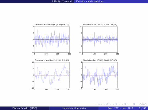
0 100 200 300-4

-2

0

2

4Simulation of an ARMA(1,1) with (-0.5;-0.5)

0 100 200 300-10

-5

0

5

10Simulation of an ARMA(1,1) with (-0.5;0.5)

0 100 200 300-10

-5

0

5

10Simulation of an ARMA(1,1) with (0.9;-0.5)

0 100 200 300-4

-2

0

2

4Simulation of an ARMA(1,1) with (0.9;0.5)



The properties of an ARMA(1,1) process are a mixture of those of anAR(1) and MA(1) processes :

The (stability) stationarity condition is the one of an AR(1) process (orARMA(1,0) process) :

|φ| < 1.

The invertibility condition is the one of a MA(1) process (orARMA(0,1) process) :

|θ| < 1.

The representation of an ARMA(1,1) process is fundamental or causalif :

|φ| < 1 and |θ| < 1.

The representation of an ARMA(1,1) process is said to be minimal andcausal if :

|φ| < 1, |θ| < 1 and φ 6= θ.



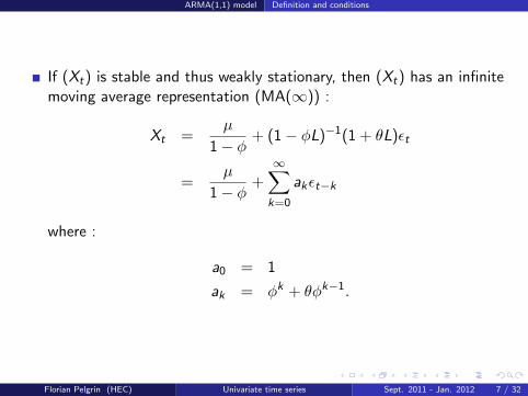
If (Xt) is stable and thus weakly stationary, then (Xt) has an infinitemoving average representation (MA(∞)) :

Xt =µ

1− φ+ (1− φL)−1(1 + θL)εt

=µ

1− φ+∞∑k=0

akεt−k

where :

a0 = 1

ak = φk + θφk−1.



If (Xt) is invertible, then (Xt) has an infinite autoregressiverepresentation (AR(∞)) :

(1− θ∗L)−1(1− φL)Xt =µ

1− θ∗+ εt

i.e.

Xt = =µ

1− θ∗+∞∑k=1

bkXt−k + εt

where θ∗ = −θ, and :

bk = −θ∗k − θ∗k−1φ.


ARMA(1,1) model Moments

1.2. Moments

Definition

Let (Xt) denote a stationary stochastic process that has a fundamentalARMA(1,1) representation, Xt = µ+ φXt−1 + εt + θεt−1. Then :

E [Xt ] =µ

1− φ≡ m

γX (0) ≡ V(Xt) =1 + 2φθ + θ2

1− φ2σ2ε

γX (1) ≡ Cov [Xt ,Xt−1] =(φ+ θ)(1 + φθ)

1− φ2σ2ε

γX (h) = φγX (h − 1) for |h| > 1.

Proof : See Appendix 1.



Definition

The autocorrelation function of an ARMA(1,1) process satisfies :

ρX (h) =

1 if h = 0

(φ+θ)(1+φθ)1+2φθ+θ2 if |h| = 1

φρX (h − 1) if |h| > 1.



The autocorrelation function of an ARMA(1,1) process exhibitsexponential decay towards zero : it does not cut off but gradually diesout as h increases.

The autocorrelation function of an ARMA(1,1) process displays theshape of that of an AR(1) process for |h| > 1.



Partial Autocorrelation :

The partial autocorrelation function of an ARMA(1,1) process willgradually die out (the same property as a moving average model).


ARMA(1,1) model Estimation

Estimation

Same techniques as before, especially those of MA models.

Yule-Walker estimator : the extended Yule-Walker equations could beused in principe to estimate the AR coefficients but the MAcoefficients need to be estimated by other means.

In the presence of moving average components, the least squaresestimator becomes nonlinear and the corresponding estimator is theconditional nonlinear least squares estimator (see estimation ofMA(q) models). It has to be solved with numerical methods.

Taking explicit distributional assumption for the error term, theconditional or exact maximum likelihood estimator can be computed(using also numerical or optimization methods).

Other methods are also available : the Kalman filter, the generalizedmethod of moments, etc.


ARMA(1,1) model Estimation

Estimation of ARMA(p,q) models (true DGP: µ = 0, φ = 0.9, and θ = 0.5)

Coefficient Std. Error t-Statistic p-value. Akaike info criterion Schwarz criterion

ARMA(1,1) C 0.4532 0.7558 0.5996 0.5490 2.8841 2.9134

AR(1) 0.9112 0.0184 49.4884 0.0000 MA(1) 0.4639 0.0409 11.3368 0.0000

ARMA(2,2) C 0.3137 0.6942 0.4518 0.6516 2.8865 2.9288

AR(1) 1.4836 0.2655 5.5879 0.0000 AR(2) -0.5230 0.2422 -2.1598 0.0313 MA(1) -0.1233 0.2666 -0.4625 0.6439 MA(2) -0.2837 0.1245 -2.2784 0.0231

ARMA(2,1) 0.3941 0.7431 0.5303 0.5961 2.8857 2.9195

AR(1) 0.8581 0.0964 8.8992 0.0000 AR(2) 0.0491 0.0937 0.5244 0.6002 MA(1) 0.5047 0.0843 5.9848 0.0000

AR(2) C 0.4276 0.6628 0.6451 0.5192 2.9206 2.9459

AR(1) 1.2819 0.0419 30.5971 0.0000 AR(2) -0.3523 0.0416 -8.4649 0.0000

AR(1) C 0.2857 0.9394 0.3042 0.7611 3.0559 3.0728

AR(1) 0.9467 0.0135 70.1399 0.0000 MA(2) C 0.6545 0.2043 3.2042 0.0014 3.6527 3.6779

MA(1) 1.3803 0.0329 41.9665 0.0000 MA(2) 0.6740 0.0324 20.8027 0.0000

MA(4) C 0.6259 0.2633 2.3768 0.0178 3.2039 3.2461

MA(1) 1.4334 0.0408 35.1707 0.0000 MA(2) 1.2250 0.0657 18.6595 0.0000 MA(3) 0.8552 0.0658 12.9989 0.0000 MA(4) 0.4131 0.0407 10.1483 0.0000

Note: C, AR(j), and MA(j) are respectively the estimate of the constant term, the jth autogressive term, and the jth moving average term.


ARMA(p,q) model Definition and conditions

2. ARMA(p,q)2.1. Definition and conditions

Definition

A stochastic process (Xt)t∈Z is said to be a mixture autoregressive movingaverage model of order p and q, ARMA(p,q), if it satisfies the followingequation :

Xt = µ+ φ1Xt−1 + · · ·+ φpXt−p + εt + θ1εt−1 + · · ·+ θqεt−q ∀tΦ(L)Xt = µ+ Θ(L)εt

where θq 6= 0, φp 6= 0, µ is a constant term, (εt)t∈Z is a weak white noiseprocess with expectation zero and variance σ2

ε (εt ∼WN(0, σ2ε )),

Φ(L) = 1− φ1L− · · · − φpLp and Θ(L) = 1 + θ1L + · · ·+ θqLq.



Main idea of ARMA(p,q) models

Approximate Wold form of stationary time series by parsimoniousparametric models

AR and MA models can be cumbersome because one may need ahigh-order model with many parameters to adequately describe thedata dynamics (see the effective Fed fund rate application)

By mixing AR and MA models into a more compact form, the numberof parameters is kept small...



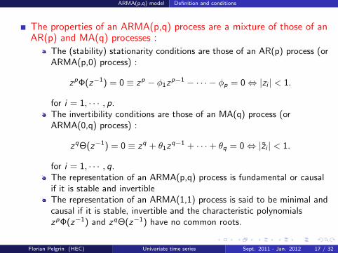
The properties of an ARMA(p,q) process are a mixture of those of anAR(p) and MA(q) processes :

The (stability) stationarity conditions are those of an AR(p) process (orARMA(p,0) process) :

zpΦ(z−1) = 0 ≡ zp − φ1zp−1 − · · · − φp = 0⇔ |zi | < 1.

for i = 1, · · · , p.The invertibility conditions are those of an MA(q) process (orARMA(0,q) process) :

zqΘ(z−1) = 0 ≡ zq + θ1zq−1 + · · ·+ θq = 0⇔ |zi | < 1.

for i = 1, · · · , q.The representation of an ARMA(p,q) process is fundamental or causalif it is stable and invertibleThe representation of an ARMA(1,1) process is said to be minimal andcausal if it is stable, invertible and the characteristic polynomialszpΦ(z−1) and zqΘ(z−1) have no common roots.



DefinitionThe representation of a mixture autoregressive moving average process of order p and qdefined by :

Xt = µ+ φ1Xt−1 + · · ·+ φpXt−p + εt + θ1εt−1 + · · ·+ θqεt−q,

is said to be a minimal causal (fundamental) representation—(εt) is the innovationprocess—if :

(i) All the roots of the characteristic equation associated to Φzp − φ1z

p−1 − · · · − φp = 0 are of modulus less than one, |zi | < 1 for i = 1, · · · , p ;

(ii) All the roots of the characteristic equation associated to Θzq + θ1z

q−1 + · · ·+ θq = 0 are of modulus less than one, |zi | < 1 for i = 1, · · · , q ;

(iii) The characteristic polynomials zpΦ(z−1) and zqΘ(z−1) have no common roots.



If (Xt) is stable and thus weakly stationary, then (Xt) has an infinitemoving average representation (MA(∞)) :

Xt =µ

1−∑p

k=1 φk+ Φ(L)−1(1 + θL)εt

=µ

1−∑p

k=1 φk+∞∑k=0

akεt−k

where :

a0 = 1∞∑k=0

|ak | <∞



If (Xt) is invertible, then (Xt) has an infinite autoregressiverepresentation (AR(∞)) :

Θ(L)−1Φ(L)Xt =µ

1−∑q

k=1 θ∗k

+ εt

i.e.

Xt = =µ

1−∑q

k=1 θ∗q

+∞∑k=1

bkXt−k + εt

where θ∗k = −θk .


ARMA(p,q) model Moments

2.2. Moments of an ARMA(p,q)

The properties of the moments of an ARMA(p,q) are also a mixtureof those of an AR(1) and MA(1) processes.

The mean is the same as the one of an AR(p) model (with a constantterm) :

E(Xt) =µ

1−∑p

k=1 φk≡ m.


ARMA(p,q) model Moments

Autocorrelation :

The autocorrelation function of an ARMA(p,q) process exhibitsexponential decay towards zero : it does not cut off but gradually diesout as h increases (possibly damped oscillations.

The autocorrelation function of an ARMA(p,q) process displays theshape of that of an AR(p) process for |h| > max(p, q + 1).

Partial Autocorrelation : The partial autocorrelation function of anARMA(p,q) process will gradually die out (the same property as aMA(q) model).


ARMA(p,q) model Estimation

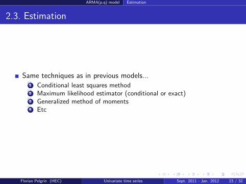
2.3. Estimation

Same techniques as in previous models...1 Conditional least squares method2 Maximum likelihood estimator (conditional or exact)3 Generalized method of moments4 Etc


Application

3. Application

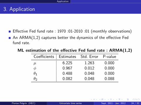
Effective Fed fund rate : 1970 :01-2010 :01 (monthly observations)

An ARMA(1,2) captures better the dynamics of the effective Fedfund rate.

ML estimation of the effective Fed fund rate : ARMA(1,2)

Coefficients Estimates Std. Error P-value

µ 6.225 1.263 0.000φ 0.967 0.012 0.000θ1 0.488 0.048 0.000θ2 0.082 0.048 0.088


Application

Effective Fed fund rate: ARMA(1,2) specification

-8

-6

-4

-2

0

2

4

0

5

10

15

20

1970 1975 1980 1985 1990 1995 2000 2005

Residual Actual Fitted


Application

Effective Fed fund rate: diagnostics of the ARMA(1,2) specification

0.4

0.5

0.6

0.7

0.8

0.9

1.0

2 4 6 8 10 12 14 16 18 20 22 24

Actual Theoretical

Aut

ocor

rela

tion

-0.5

0.0

0.5

1.0

2 4 6 8 10 12 14 16 18 20 22 24

Actual Theoretical

Par

tial au

toco

rrel

atio

n


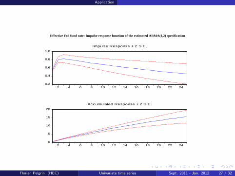
Application

Effective Fed fund rate: Impulse response function of the estimated ARMA(1,2) specification

0.2

0.4

0.6

0.8

1.0

2 4 6 8 10 12 14 16 18 20 22 24

Impulse Response ± 2 S.E.

0

5

10

15

20

2 4 6 8 10 12 14 16 18 20 22 24

Accumulated Response ± 2 S.E.


Appendix

4. Appendix

1. Moments of an ARMA(1,1).


Appendix

1. Moments of an ARMA(1,1)

The properties of the moments of an ARMA(1,1) are a mixture ofthose of an AR(1) and MA(1) processes.

The mean is the same as the one of an AR(1) model (with a constantterm) :

E(Xt) = E (µ+ φXt−1 + εt + θεt−1)

= µ+ φE(Xt−1) + E(εt) + θE(εt−1)

= µ+ φE(Xt)

since E(Xt) = E(Xt−j) for all j (stationarity property) andE(εt−j) = 0 for all j(white noise). Therefore,

E(Xt) =µ

1− φ≡ m.


Appendix

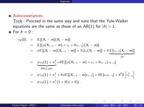
AutocovariancesTrick : Proceed in the same way and note that the Yule-Walkerequations are the same as those of an AR(1) for |h| > 1.

For h = 0 :

γX (0) = E [(Xt −m)(Xt −m)]

= E [(φ(Xt−1 −m) + εt + θεt−1) (Xt −m)]

= φE [(Xt −m)(Xt−1 −m)] + E [εt(Xt −m)] + θE [εt−1(Xt −m)]︸︷︷︸6=0

= φγX (1) + σ2ε︸︷︷︸

AR(1) part

+θE [(φ(Xt−1 −m) + εt + θεt−1) εt−1]

= φγX (1) + σ2ε + θφE [(Xt−1 −m)εt−1] + θE [εtεt−1] + θ2E

[ε2t−1

]= φγX (1) + σ2

ε (1 + θ(φ+ θ)) .


Appendix

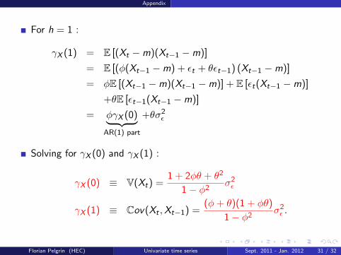
For h = 1 :

γX (1) = E [(Xt −m)(Xt−1 −m)]

= E [(φ(Xt−1 −m) + εt + θεt−1) (Xt−1 −m)]

= φE [(Xt−1 −m)(Xt−1 −m)] + E [εt(Xt−1 −m)]

+θE [εt−1(Xt−1 −m)]

= φγX (0)︸︷︷︸AR(1) part

+θσ2ε

Solving for γX (0) and γX (1) :

γX (0) ≡ V(Xt) =1 + 2φθ + θ2

1− φ2σ2ε

γX (1) ≡ Cov(Xt ,Xt−1) =(φ+ θ)(1 + φθ)

1− φ2σ2ε .


Appendix

For |h| > 1 :

γX (h) = E [(Xt −m)(Xt−h −m)]

= E [(φ(Xt−1 −m) + εt + θεt−1) (Xt−h −m)]

= φE [(Xt−1 −m)(Xt−h −m)] + E [εt(Xt−h −m)]

+θE [εt−1(Xt−h −m)]

= φγX (h − 1)︸︷︷︸AR(1) part

since E [εt−j(Xt−h −m)] = 0 for all h > j—(εt) is the innovationprocess.The expression of the autocovariance of order h displays the samedifference or recurrence equation as in an AR(1) model—only theinitial value γX (1) changes !


Documents

Lecture 2: ARMA(p,q) models (part 3) - math.unice.frfrapetti/CorsoP/chapitre_23_IMEA_1.pdf · Introduction Road map 1 ARMA(1,1) model De nition and conditions Moments Estimation 2