Lecture 18 Cointegration - Bauer College of Business model appears to have good fit well even though it is misspecified. ... • This is called a vector error correction model (VECM)

RS – EC2 - Lecture 18

1

1

Lecture 18Cointegration

• Suppose yt and xt are I(1). We regress yt against xt. What happens?

• The usual t-tests on regression coefficients can show statistically significant coefficients, even if in reality it is not so.

• This the spurious regression problem (Granger and Newbold (1974)).

• In a Spurious Regression the errors would be correlated and the standard t-statistic will be wrongly calculated because the variance of the errors is not consistently estimated.

Note: This problem can also appear with I(0) series –see, Granger, Hyung and Jeon (1998).

Spurious Regression


2

Examples:(1) Egyptian infant mortality rate (Y), 1971-1990, annual data, on Gross aggregate income of American farmers (I) and Total Honduran money supply (M)

ŷ = 179.9 - .2952 I - .0439 M, R2 = .918, DW = .4752, F = 95.17(16.63) (-2.32) (-4.26) Corr = .8858, -.9113, -.9445

(2). US Export Index (Y), 1960-1990, annual data, on Australian males’ life expectancy (X)

ŷ = -2943. + 45.7974 X, R2 = .916, DW = .3599, F = 315.2(-16.70) (17.76) Corr = .9570

(3) Total Crime Rates in the US (Y), 1971-1991, annual data, on Life expectancy of South Africa (X)

ŷ = -24569 + 628.9 X, R2 = .811, DW = .5061, F = 81.72(-6.03) (9.04) Corr = .9008

Spurious Regression - Examples

• Suppose yt and xt are unrelated I(1) variables. We run the regression:

• True value of β=0. The above is a spurious regression and et ∼ I(1).

• Phillips (1986) derived the following results:- not 0. It non-normal RV not necessarily centered at 0.

=> This is the spurious regression phenomenon.

-The OLS t-statistics for testing H0: β=0 diverge to ±∞ as T→ ∞. Thus, with a large enough T it will appear that β is significant.

- The usual R2 1 as T → ∞. The model appears to have goodfit well even though it is misspecified.

Spurious Regression - Statistical Implications

ttt xy

D

DD


3

• Intuition:With I(1) data sample moments converge to functions of Brownian motion (not to constants).

• Sketch of proof of Phillip’s first result.- Consider two independent RW processes for yt and xt. We regress:

- OLS estimator of β:

- Then, (not) 0. non-normal RV.

Spurious Regression - Statistical Implications

ttt xy

drrWrWdrrW

xT

xyT

yxyxxxd

T

t

T

ttt

t

)()()(ˆ1

0

11

0

22

1

22

1

2

Dp

• Given the statistical implications, the typical symptoms are: - High R2, t-values, & F-values. - Low DW values.

• Q: How do we detect a spurious regression (between I(1) series)?- Check the correlogram of the residuals.- Test for a unit root on the residuals.

• Statistical solution: When series are I(1), take first differences. Now, we have a valid regression. But, the economic interpretation of the regression changes.

. When series are I(0), modify the t-statistic:

Spurious Regression – Detection and Solutions

1/2ˆ )ˆ of cerun varian-(long ˆ where,on distributi-t tˆˆ


4

• The message from spurious regresssion: Regression of I(1) variables can produce nonsense.

Q: Does it make sense a regression between two I(1) variables?Yes, if the regression errors are I(0). That is, when the variables are cointegrated.

Spurious Regression – Detection and Solutions

• Integration: In a univariate context, yt is I(d) if its (d-1)th difference is I(0). That is, Δdyt is stationary.

=> yt is I(1) if Δyt is I(0).

• In many time series, integrated processes are considered together and they form equilibrium relationships:- Short-term and long-term interest rates- Inflation rates and interest rates.- Income and consumption

Idea: Although a time series vector is integrated, certain linear transformations of the time series may be stationary.

Cointegration


5

• An mx1 vector time series Yt is said to be cointegrated of order (d,b), CI(d,b) where 0<bd, if each of its component series Yit is I(d) but some linear combination ’Yt is I(db) for some constant vector ≠0.

•: cointegrating vector or long-run parameter.

• The cointegrating vector is not unique. For any scalar cc ’Yt = *’Yt is I(db) ~ I(db)

• Some normalization assumption is required to uniquely identify . Usually, 1=(the coefficient of the first variable) is normalized to 1.

• The most common case is d=b=1.

Cointegration - Definition

• If the mx1 vector time series Yt contains more than 2 components, each being I(1), then there may exist k (<m) linearly independent 1xm vectors 1’, 2’,…, k’, such that ’Yt ~ I(0) kx1 vector process, where = (1,2’,…, k) is a kxm cointegrating matrix.

• Intuition for I(1) case’Yt forms a long-run equilibrium. It cannot deviate too far from the equilibrium, otherwise economic forces will operate to restore the equilibrium.

• The number of linearly independent cointegrating vectors is called the cointegrating rank:

Yt is cointegrated of rank k.

If the mx1 vector time series Yt is CI(k,1) with 0<k<m CI vectors, then there are m-k common I(1) stochastic trends.

Cointegration - Definition


6

Example: Consider the following system of processes

where the error terms are uncorrelated WN processes. Clearly, all the 3 processes are individually I(1).

- Let yt=(x1t,x2t,x3t)’ and =(1,1,2)’ => ’ yt=ε1t ~I(0).

Note: The coefficient for x1 is normalized to 1.

- Another CI relationship: x2t & x3t.. Let *=(0 1,-3)’ =>’yt =ε2t~I(0).

- 2 independent C.I. vectors => 1 common ST: Σt ε3t.

Cointegration - Example

ttt

ttt

tttt

xx

xx

xxx

31,33

2332

132211

VAR with Cointegration

• Let Yt be mx1. Suppose we estimate VAR(p)

or

• Suppose we have a unit root. Then, we can write

• This is like a multivariate version of the ADF test:

tptptt aYYY 11

.aYBY t1tt

BBB * 11

12

.1

1 t

p

iititt aYYY


7


• Rearranging the equation

where Rank((1)I)<m. There are two cases:

1. (1)= I, then we have m independent unit roots, so there is nocointegration, and we should run the VAR in differences.

2. 0< Rank((1)I) = k < m, then we can write (1)I =’ where and are mxk. The equation becomes:

• This is called a vector error correction model (VECM). Part of Granger Representation Theorem: “Cointegration implies an ECM.”

.B1 t1t*

1t aYYIYt

.B tt*

t aYYYt 11

13


• Note: If we have cointegration, but we run OLS in differences,then the modeled is misspecified and the results will be biased.

• Q: What can you do?- If you know the location of the unit roots and cointegrationrelations, then you can run the VECM by doing OLS of Yt on lagsof Y and ’Yt1.- If you know nothing, then you can either

(i) run OLS in levels, or(ii) test (many times) to estimate cointegrating relations. Then, run VECM.

• The problem with this approach is that you are testing many timesand estimating cointegrating relationships. This leads to poor finitesample properties.

14


8

Residual Based Tests of the Null of No CI

• Procedures designed to distinguish a system without cointegration from a system with at least one cointegrating relationship; they do not estimate the number of cointegrating vectors (the k).

• Tests are conditional on pretesting (for unit roots in each variable).

• There are two cases to consider.

• CASE 1 - Cointegration vector is pre-specified/known (say, from economic theory) : Construct the hypothesized linear combination that is I(0) by theory; treat it as data. Apply a DF unit root test to that linear combination.

• The null hypothesis is that there is a unit root, or no cointegration.

15

• CASE 2 - Cointegration vector is unknown. It should be estimated.Thus, if there exists a cointegrating relation, the coefficient on Y1t is nonzero, allowing us to express the “static regression equation as

• Then, apply a unit root test to the estimated OLS residual from estimation of the above equation, but- Include a constant in the static regression if the alternative allows for a nonzero mean in ut

- Include a trend in the static regression if the alternative is stochastic cointegration -i.e., a nonzero trend for A’Yt.

Note: Tests for cointegration using a prespecified cointegrating

vector are generally more powerful than tests estimating the vector.

t2t1t uY Y

16

Residual Based Tests of the Null of No CI


9

• Steps in cointegration test procedure:

1. Test H0(unit root) in each component series Yit individually, using the univariate unit root tests, say ADF, PP tests.

2. If the H0 (unit root) cannot be rejected, then the next step is to test cointegration among the components, i.e., to test whether ’Yt is I(0).

• In practice, the cointegration vector is unknown. One way to test the existence of cointegration is the regression method –see, Engle and Granger (1986) (EG).

• If Yt=(Y1t,Y2t,…,Ymt) is cointegrated, ’Yt is I(0) where =(1, 2,…, m). Then, (1/1) is also a cointegrated vector where 10.

17

Engle and Granger Cointegration


• EG consider the regression model for Y1t

where Dt: deterministic terms.

• Check whether t is I(1) or I(0):

- If t~I(1), then Yt is not cointegrated.

- If t~I(0), then Yt is cointegrated with a normalized cointegrating vector ’=(1,1,…, m1) .

• Steps:

1. Run OLS. Get estimate

2. Use residuals et for unit root testing using the ADF or PP tests without deterministic terms (constant or constant and trend). 18

tmtmttt YYDY 1211

.ˆ,,ˆ1,ˆ 1m1


10

• Step 2: Use residuals et for unit root test.

- Note:

If εt ~I(1), t-test has a non-standard distribution.

- H0 (unit root in residuals): =0 vs H1: <1 for the model

- t-statistic:

- Critical values tabulated by simulation in EG.

• We expect the usual ADF distribution would apply here. But, Phillips and Ouliaris (PO) (1990) show that is not the case. 19

)0(~ if on,distributiˆ It td

i

t

p

jjtjtt a

1

11


ˆ

ˆ

st

• Phillips and Ouliaris (PO) (1990) show that the ADF and PP unit root tests applied to the estimated cointegrating residual do not have the usual DF distributions under H0 (no-cointegration).

• Due to the spurious regression phenomenon under H0, the distribution of the ADF and PP unit root tests have asymptotic distributions that are functions of Wiener processes that depends on:

- The deterministic terms, Dt, in the regression used to estimate - The number of variables, (m-1), in Y2t.

• PO tabulated these distributions. Hansen (1992) improved on these distributions, getting adjustments for different DGPs with trend and/or drift/no drift.

20

EG Cointegration – PO Distribution


11

• EG propose LS to consistently estimate a normalized CI vector.But, the asymptotic behavior of the LS estimator is non-standard.

• Stock (1987) and Phillips (1991) get the following results:

- T ( − ) non-normal RV not necessarily centered at 0.

- The LS estimate . Convergence is at rate T, not usual T1/2. => We say is super consistent.

- is consistent even if the other (m-1) Yt’s are correlated with εt.

=> No asymptotic simultaneity bias.

- The OLS formula for computing aVar( ) is incorrect

=>usual OLS standard errors are not correct.

- Even though the asymptotic bias →0, as T→∞, can be substantially biased in small samples. LS is also not efficient.

21

EG Cointegration – Least Square Estimator

D

p

• The bias is caused by εt. If εt ~ WN, there is no asymptotic bias.

• The above results point out that the LS estimator of the CI vector could be improved upon.

• Stock and Watson (1993) propose augmenting the CI regression of Y1t against the rest (m-1) elements in Yt , say Yt* with appropriate deterministic terms Dt, with p leads and lags of ΔYt*.

• Estimate the augmented regression by OLS. The resulting estimator of is called the dynamic OLS estimator or DOLS.

• It is consistent, asymptotically normally distributed and, under certain assumptions, efficient. 22

EG Cointegration – Least Square Estimator


12

• Consider a bivariate I(1) vector Yt = (Y1t, Y2t) .

- Assume that Yt is cointegrated with CI =(1,-2). That is,

’Yt = Y1t - 2 Y2t ~ I(0).

- Suppose we have a consistent estimate (or DOLS) of .

- We are interested in estimating the VECM for ΔY1t and ΔY2t using:

ΔY1t = c1 + β1( Y1t - 2 Y2t) + Σj ψ11,j ΔY1t-j+ Σj ψ12,j ΔY2t-j + u1t

ΔY2t= c2 + β2( Y1t - 2 Y2t) + Σj ψ21,j ΔY1t-j+ Σj ψ22,j ΔY2t-j + u2t

• is super consistent. It can be treated as known in the ECM. The estimated disequilibrium error ’Yt =Y1t-2^ Y2t may be treated like the known ’Yt .

• All variables are I(0), we can use OLS (or SUR to gain efficiency.)23

EG Cointegration – Estimating VECM with LS

• The EG procedure works well for a single equation, but it does not extend well to a multivariate VAR model.

• Consider a levels VAR(p) model:

where Yt is a time series mx1 vector. of I(1) variables.

• The VAR(p) model is stable if

det(In − Φ1z − · · · − Φpzp) = 0

has all roots outside the complex unit circle.

• If there are roots on the unit circle then some or all of the variables in Yt are I(1) and they may also be cointegrated. 24

tptpttt YYDY 11

Johansen Tests


13

• If Yt is cointegrated, then the levels VAR representation is not the right one, since the cointegrating relations are not explicitly apparent.

• The CI relations appear if the VAR is transformed to the VECM.

• For these cases, Johansen (1988, 1991) proposed two tests: The trace test and the maximal eigenvalue test. They are based on Granger’s (1981) ECM representation. Both tests are easy to implement.Example: Trace test simple idea:(1) Assume εt are multivariate N(0, .). Estimate the VECM by ML, under various assumptions:- trend/no trend and/or drift/no drift- the number k of CI vectors, (2) Compare models using likelihood ratio tests. 25

Johansen Tests

• Consider the VECM

where - Dt : vector of deterministic variables (constant, trends, and/orseasonal dummy variables);- are m×m matrices;- = A’ is the long-run impact matrix; A and are m×k matrices;- t are i.i.d. Nm(0, ) errors; and - det( ) has all of its roots outside the unit circle.

• In this framework, CI happens when has reduced rank. This is the basis of the test: By checking the rank of , we can determine if the system is CI.

26

1 , j = 1, , p-1j jI

1

j

1

Bp

j

j

I

t

p

j jtjttt YYDY

1

110

Johansen Tests - Intuition


14

• We can also write the ECM using the alternative representation as

where the ECM term is at lag t-p. Including a constant and or a deterministic trend in the ECM is also possible.

• Back to original VECM(p).

- Let Z0t= ΔYt , Z1t= Yt-1 and Z2t= (ΔYt-1 ,..., ΔYt-p-1, Dt)’

• Now, we can write: Z0t= A’ Yt-1 + Ψ Z2t+ εt

where Ψ =(Γ1 Γ2 ... Γp Γ0 ).

• If we assume a distribution for εt, we can write the likelihood. 27

t

p

j jtjpttt YYDY

1

10 **


• Assume the VECM errors are independent Nm(0, ) distribution,. Then, given the CI restrictions on the trend and/or drift/no drift parameters, the likelihood Lmax(k) is a function of the CI rank k.

• The trace test is based on the log-likelihood ratio:LR= 2 ln[Lmax(Unrestricted)/Lmax(Restricted)],

which is done sequentially for k = m-1,...,1,0.

• The name comes from the fact that the test statistics involved are the trace (the sum of the diagonal elements) of a diagonal matrix of generalized eigenvalues.

• The test examines the H0: CI rank ≤ k, vs. H1: CI rank > k.- If the LR is greater than the critical value for a certain rank, then the H0 is rejected.

28



15

• Johansen concentrates all the parameter matrices in the likelihood function out, except for the matrix A. Then, he shows that the MLE of A can be derived as the solution of a generalized eigenvalue problem.

• LR tests of hypotheses about the number of CI vectors can then be based on these eigenvalues. Moreover, Johansen (1988) also proposes LR tests for linear restrictions on these CI vectors.

• Note: The factorization = A’ is not unique since for any k × knonsingular matrix F we have:

A’ = F F-1 A’ =( F) (F-1A’ ) = *A*’=> The factorization = A’ only identifies the space spanned by the CI relations. To get a unique and A’ , we need more restrictions. Usually, we normalize. Finding a good way to do this is hard.

29


• The Johansen tests examine H0: Rank() ≤ k, where k is less than m.

• The unrestricted CI VECM is denoted H(r). The I(1) model H(k) can be formulated as the condition that the rank of is less than or equal to k. This creates a nested set of models

- H(m) is the unrestricted, stationary VAR model or I(0) model - H(0) non-CI VAR (restriction =0) => VAR model for differences.

• This nested formulation is convenient for developing a sequential procedure to test for the number k of CI relationships.

30

mHkHH 0

Johansen Tests – Sequential Tests


16

• Sequential tests:i. H0: k=0, cannot be rejected →stop →k=0

(at most zero coint) rejected →next testii. H0: k<=1, cannot be rejected →stop→k=1

(at most one coint) rejected →next testiii. H0: k2, cannot be rejected →stop→k=2

(at most two coint) rejected →next test

• Possible outcomes:- Rank k = m => All variables in x are I(0), not an interesting case.- Rank k = 0 => No linear combinations of Y that are I(0). =0.

Model on differenced series- Rank k (m-1) => Up to (m-1) cointegration relationships ´Yt

31


• The Johansen tests examine H0: Rank() ≤ k, where k is less than m.

Recall, Rank() = number of non-zero eigenvalues of .

• Since = A’ , it is equivalent to test that A and are of full column rank k, the number of independent CI vectors that forms the matrix A.

• It turns out the LR test statistic is the trace of a diagonal matrix of generalized eigenvalues from .

• These eigenvalues also happen to equal the squared canonical correlationsbetween ΔYt and Yt−1, corrected for lagged ΔYt and Dt. They arebetween 0 and 1.

32



17

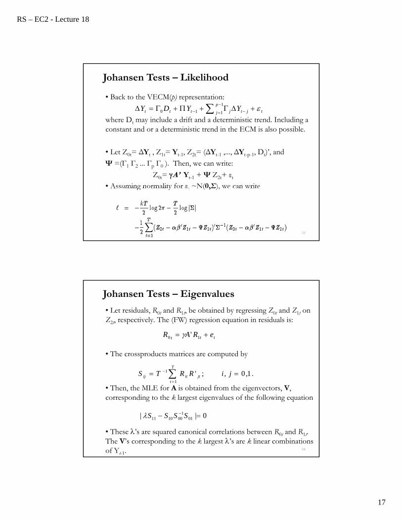
• Back to the VECM(p) representation:

where Dt may include a drift and a deterministic trend. Including a constant and or a deterministic trend in the ECM is also possible.

• Let Z0t= ΔYt , Z1t= Yt-1, Z2t= (ΔYt-1 ,..., ΔYt-p-1, Dt)’, and

Ψ =(Γ1 Γ2 ... Γp Γ0 ). Then, we can write:

Z0t= A’ Yt-1 + Ψ Z2t+ εt

• Assuming normality for εt ~N(0,Σ), we can write

33

Johansen Tests – Likelihood

t

p

j jtjttt YYDY

1

110

• Let residuals, R0t and R1t, be obtained by regressing Z0t and Z1t on Z2t, respectively. The (FW) regression equation in residuals is:

• The crossproducts matrices are computed by

• Then, the MLE for A is obtained from the eigenvectors, V, corresponding to the k largest eigenvalues of the following equation

• These ’s are squared canonical correlations between R0t and R1t. The V’s corresponding to the k largest ’s are k linear combinations of Yt-1. 34

Johansen Tests – Eigenvalues

ttt eRAR 10 '

.1,0,;'1

1

jiRRTST

tjtitij

0|| 011

001011 SSSS


18

• The eigenvectors corresponding to the k largest ’s are the k linear combinations of Yt-1, which have the largest squared partial correlations with the I(0) process, after correcting for lags and Dt.

• Computations.

- ’s. Instead of using

pre and post multiply the expression by S11-1/2 (Cholesky

decomposition of S11). Then, we have a standard eigenvalue problem.

=>

- V. The eigenvectors (say, ui,) are usually reported normalized, such that ui ’ui = 1. Then, in this case, we need to use vi =S11

-1/2 ui

That is, we normalized the eigenvectors such that S11 = I.35

0|| -1/21101

10010

-1/211 SSSSSI

0,|| 011

001011 SSSS


• The tests are based on the ’s from

• Interpretation of the eigenvalue equation.

Using F-W, we regress R0t on R1t, to estimate = A’ . That is

Note that

The ’s produced look like eigenvalues of [ ] after pre-multiplying by S11

-1/2 and post-multiplying by S00-1/2, a normalization.

• Johansen also finds:36

0.|| -1/21101

10010

-1/211 SSSSSI

.ˆ10

-1/211 SS

)ˆ)(ˆ( -1/211

2/100

2/100

-1/211

1/211

-11101

2/100

2/10010

-111

1/211

-1/21101

10010

-1/211 SSSSSSSSSSSSSSSSS


]v,...,v,[vAA k21MLE

.Aˆ 01SMLE


19

• Johansen (1988) suggested two tests for H0: At most k CI vectors:

- The trace test

- The maximal eigenvalue test.

• Both tests are based on the ’s from

They are LR tests, but they do not have the usual χ2 asymptotic distribution under H0. They have non-standard distributions.

37

Johansen Tests – Trace Statistic

0.|| -1/21101

10010

-1/211 SSSSSI

• The trace test:

where denotes the descending ordered eigenvalues

of

Note: The LRtrace statistic is expected to be close to zero if there is at most k (linearly independent) CI vectors.

• If LRtrace (k)>CV(for rank k), then H0 (CI Rank=k) is rejected.

• If Rank() = k0 then should all be close to 0. TheLRtrace(k0) should be small since ln(1 − ) ≈ 0 for i > k0.

38

Johansen Trace Test

i

mk ˆ,,ˆ

10

m

kiitrace TkLR

1

ˆ1lnln2)(

ˆi

0.|| 011

001011 SSSS0ˆ

1 m


20

• Under H0, the asymptotic distribution of LRtrace(k0) is not χ2. It is a multivariate version of the DF unit root distribution, which depends on the dimension m-k0 and the specification of Dt.

• The statistic ln has a limiting distribution, which can be expressed in terms of a mk dimensional Brownian motion W as

is the Brownian motion itself (W), or the demeaned or detrended W, according to the different specifications for Dt in the VECM

• Using simulations, critical values are tabulated in Johansen (1988, Table 1) and in Osterwald-Lenum (1992) for m-k0 = 1, . . . , 10.

39

Johansen Trace Test – Distribution

• An alternative LR statistic, given by

is called the maximal eigenvalue statistic. It examines the null hypothesis of k cointegrating vectors versus the alternative k+1 CI vectors. That is, H0: CI rank = k, vs. H1: CI rank = k+1.

• Similar to the trace statistic, the asymptotic distribution of this LR is not statistic the usual χ2. It is given by the maximum of the stochastic matrix in

which depends on the dimension m−k0 and the specification of the deterministic terms, Dt. See Osterwald-Lenum (1992) for CVs.

40

1maxˆ1lnln2)( kTkLR

Johansen Maximal EigenvalueTest


21

• Suppose we find Rank() = k, 0 <k<m. Then, the CI VECM:

• This is a reduced rank multivariate regression. Johansen derived the ML estimation of the parameters under the reduced rank restriction

Rank() = k.

Recall that A = AMLE is given by the eigenvectors associated with the ’s.

• The MLEs of the remaining parameters are obtained by OLS of

41

ML Estimation of the CI VECM

tp

j jtjttt YYADY

1

110 '

tp

j jtjttt YYADY

1

110 'ˆ

• The factorization = A’ is not unique. The columns of AMLE may be interpreted as linear combinations of the underlying CI relations.

• For interpretation, it is convenient to normalize the CI vectors bychoosing a specific coordinate system in which to express the variables.

• Johansen suggestion: Solve for the triangular representation of the

CI system. The resulting normalized CI vector is denoted Ac,MLE.

• The normalization of A affects the MLE of but not the MLEs of the other parameters in the VECM.

• Properties of Ac,MLE: asymptotically normal and super consistent. 42

ML Estimation of the CI VECM


22

• The Johansen MLE procedure only produces an estimate of the basis for the space of CI vectors.

• It is often of interest to test if some hypothesized CI vector lies in the space spanned by the estimated basis:

H0: A = [A0 φ] Rank() ≤ k

A0: s×m matrix of hypothesized CI vectors

φ : (k-s)×m matrix of unspecified CI vectors

• Johansen shows that a LR test can be computed, which is asymptotically distributed as a χ2 with s(m-k) degrees of freedom.

43

ML Estimation of the CI VECM - Testing

• Following Johansen (1988, 1991) one can choose a set of vectors A┴ such that the matrix {A, A┴} has full rank and A’ A┴ = 0. [A┴read “A perp”]

• That is, the mx(m-k) matrix A┴ is orthogonal to the matrix A=> columns of A┴ are orthogonal to the columns of A.

• The vectors A┴ Yt represents the non-CI part of Yt. We call A┴ the common trends loading matrix.

• We refer to the space spanned by A┴ Yt as the unit root space of Yt.

• Reference:Stock and Watson (1988). 44

Common Trends


23

• The EG’s two-step estimator is simple, but not asymptotically efficient. Several papers proposed improved, efficient methods.

- Phillips (1991): Regression in the spectral domain.

- Phillips and Loretan (1991): Non-linear EC estimation.

- Phillips and Hansen (1990): IV regression with a correction a la PP.

- Saikkonen (1991): Inclusion of leads and lags in the lag-polynomials of the ECM in order to achieve asymptotic efficiency

- Saikkonen (1992): Simple GLS type estimator

- Park's (1991) CCR estimator transforms the data so that OLS afterwards gives asymptotically efficient estimators

- Engle and Yoo (1991): A 3 step estimator for the EG procedure.

• From all of these estimators, we can get a t-values for the EC term.45

Asymptotic Efficient Single Equation Methods

Example (Lütkepohl (1993)): m=4 U.S. quarterly macro variables: Log real M1, Log output, 91-day T-bill yield, 20-year T-bond yield.

Period: 1954 to 1987

• Analysis:

1) Dickey-Fuller unit root test

2) Johansen cointegration test integrated order 2,

3) VECM(2) estimation.

• SAS Codeproc varmax data=us_money;

id date interval=qtr;

model y1-y4 / p=2 lagmax=6 dftest print=(iarr(3)) cointtest=(johansen=(iorder=2)) ecm=(rank=1 normalize=y1);

cointeg rank=1 normalize=y1 exogeneity;

run; 46

Example: Cointegration - Lütkepohl (1993) - SAS


24

• Dickey-Fuller Unit Root TestsVariable Type Rho Pr < Rho Tau Pr < Tau

y1 Zero Mean 0.05 0.6934 1.14 0.9343

Single Mean -2.97 0.6572 -0.76 0.8260

Trend -5.91 0.7454 -1.34 0.8725

y2 Zero Mean 0.13 0.7124 5.14 0.9999

Single Mean -0.43 0.9309 -0.79 0.8176

Trend -9.21 0.4787 -2.16 0.5063

y3 Zero Mean -1.28 0.4255 -0.69 0.4182

Single Mean -8.86 0.1700 -2.27 0.1842

Trend -18.97 0.0742 -2.86 0.1803

y4 Zero Mean 0.40 0.7803 0.45 0.8100

Single Mean -2.79 0.6790 -1.29 0.6328

Trend -12.12 0.2923 -2.33 0.417047

Example: Lütkepohl (1993) – SAS: DF Tests

Note: In all series, we cannot reject H0

(unit root).

48

• The fitted VECM(2) is given as

Example: Lütkepohl (1993) – SAS: VECM(2)


25

49

Cointegration Rank Test for I(2)

r\k-r-s 4 3 2 1Traceof I(1)

5% CV of I(1)

0 384.60903 214.37904 107.93782 37.02523 55.9633 47.21

1 219.62395 89.21508 27.32609 20.6542 29.38

2 73.61779 22.13279 2.6477 15.34

3 38.29435 0.0149 3.84

5% CV I(2) 47.21000 29.38000 15.34000 3.84000


• Note: System is cointegrated in rank 1 with integrated order 1.

• The factorization = A’

50


A (Beta in SAS)

Variable 1 2 3 4

y1 1.00000 1.00000 1.00000 1.00000

y2 -0.46458 -0.63174 -0.69996 -0.16140

y3 14.51619 -1.29864 1.37007 -0.61806

y4 -9.35520 7.53672 2.47901 1.43731

(Alpha in SAS)

Variable 1 2 3 4

y1 -0.01396 0.01396 -0.01119 0.00008

y2 -0.02811 -0.02739 -0.00032 0.00076

y3 -0.00215 -0.04967 -0.00183 -0.00072

y4 0.00510 -0.02514 -0.00220 0.00016

Normalization y1


26

• The factorization = A’

51

Long-Run ParameterBeta Estimates When

RANK=1

Variable 1

y1 1.00000

y2 -0.46458

y3 14.51619

y4 -9.35520

Adjustment CoefficientAlpha Estimates When

RANK=1

Variable 1

y1 -0.01396

y2 -0.02811

y3 -0.00215

y4 0.00510


Covariances of Innovations

Variable y1 y2 y3 y4

y1 0.00005 0.00001 -0.00001 -0.00000

y2 0.00001 0.00007 0.00002 0.00001

y3 -0.00001 0.00002 0.00007 0.00002

y4 -0.00000 0.00001 0.00002 0.00002

• Covariance Matrix

52

Schematic Representation of Cross Correlationsof Residuals

Variable/Lag

0 1 2 3 4 5 6

y1 ++.. .... ++.. .... +... ..-- ....

y2 ++++ .... .... .... .... .... ....

y3 .+++ .... +.-. ..++ -... .... ....

y4 .+++ .... .... ..+. .... .... ....

+ is > 2*std error, - is < -2*std error, . is between

Portmanteau Test for Cross Correlationsof Residuals

Up To Lag DF Chi-Square Pr > ChiSq

3 16 53.90 <.0001

4 32 74.03 <.0001

5 48 103.08 <.0001

6 64 116.94 <.0001

Example: Lütkepohl (1993) – SAS: Diagnostics


27

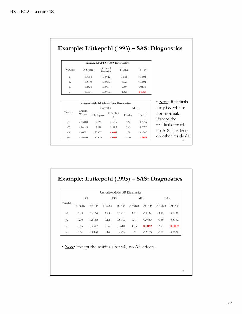
• Note: Residuals for y3 & y4 are non-normal. Except the residuals for y4, no ARCH effects on other residuals.

53

Univariate Model ANOVA Diagnostics

Variable R-SquareStandardDeviation

F Value Pr > F

y1 0.6754 0.00712 32.51 <.0001

y2 0.3070 0.00843 6.92 <.0001

y3 0.1328 0.00807 2.39 0.0196

y4 0.0831 0.00403 1.42 0.1963

Univariate Model White Noise Diagnostics

VariableDurbinWatson

Normality ARCH

Chi-SquarePr > ChiS

qF Value Pr > F

y1 2.13418 7.19 0.0275 1.62 0.2053

y2 2.04003 1.20 0.5483 1.23 0.2697

y3 1.86892 253.76 <.0001 1.78 0.1847

y4 1.98440 105.21 <.0001 21.01 <.0001


54

Univariate Model AR Diagnostics

Variable

AR1 AR2 AR3 AR4

F Value Pr > F F Value Pr > F F Value Pr > F F Value Pr > F

y1 0.68 0.4126 2.98 0.0542 2.01 0.1154 2.48 0.0473

y2 0.05 0.8185 0.12 0.8842 0.41 0.7453 0.30 0.8762

y3 0.56 0.4547 2.86 0.0610 4.83 0.0032 3.71 0.0069

y4 0.01 0.9340 0.16 0.8559 1.21 0.3103 0.95 0.4358


• Note: Except the residuals for y4, no AR effects.


28

Testing Weak Exogeneity ofEach Variables

Variable DF Chi-Square Pr > ChiSq

y1 1 6.55 0.0105

y2 1 12.54 0.0004

y3 1 0.09 0.7695

y4 1 1.81 0.1786

• Note: Variable y1 is not weak exogeneous for the other variables, y2, y3, & y4; variable y2 is not weak exogeneous for variables, y1, y3, & y4.

Weak exogeneity Long-run non-causality


• If a variable can be taken as "given" without losing information for statistical inference, it is called weak exogenous. In the CI model, a variable do not react to a disequilibrium –i.e., the EC term.

Documents

Lecture 18 Cointegration - Bauer College of Business model appears to have good fit well even though it is misspecified. ... • This is called a vector error correction model (VECM)