Lecture 16

Quantum field theory:from phonons to photons

Field theory: from phonons to photons

In our survey of single- and “few”-particle quantum mechanics, ithas been possible to work with individual constituent particles.

However, when the low energy excitations involve coherentcollective motion of many individual particles – such as wave-likevibrations of an elastic solid...

...or where discrete underlying classical particles can not even beidentified – such as the electromagnetic field,...

...such a representation is inconvenient or inaccessible.

In such cases, it is profitable to turn to a continuum formulation ofquantum mechanics.

In the following, we will develop these ideas on background of thesimplest continuum theory: lattice vibrations of atomic chain.

Provides platform to investigate the quantum electrodynamics –and paves the way to development of quantum field theory.

Atomic chain

As a simplified model of (one-dimensional) crystal, consider chain ofpoint particles, each of mass m (atoms), elastically connected bysprings with spring constant ks (chemical bonds).

Although our target will be to construct a quantum theory ofvibrational excitations, it is helpful to first review classical system.

Once again, to provide a bridge to the literature, we will follow theroute of a Lagrangian formulation – but the connection to theHamiltonian formulation is always near at hand!

Classical chain

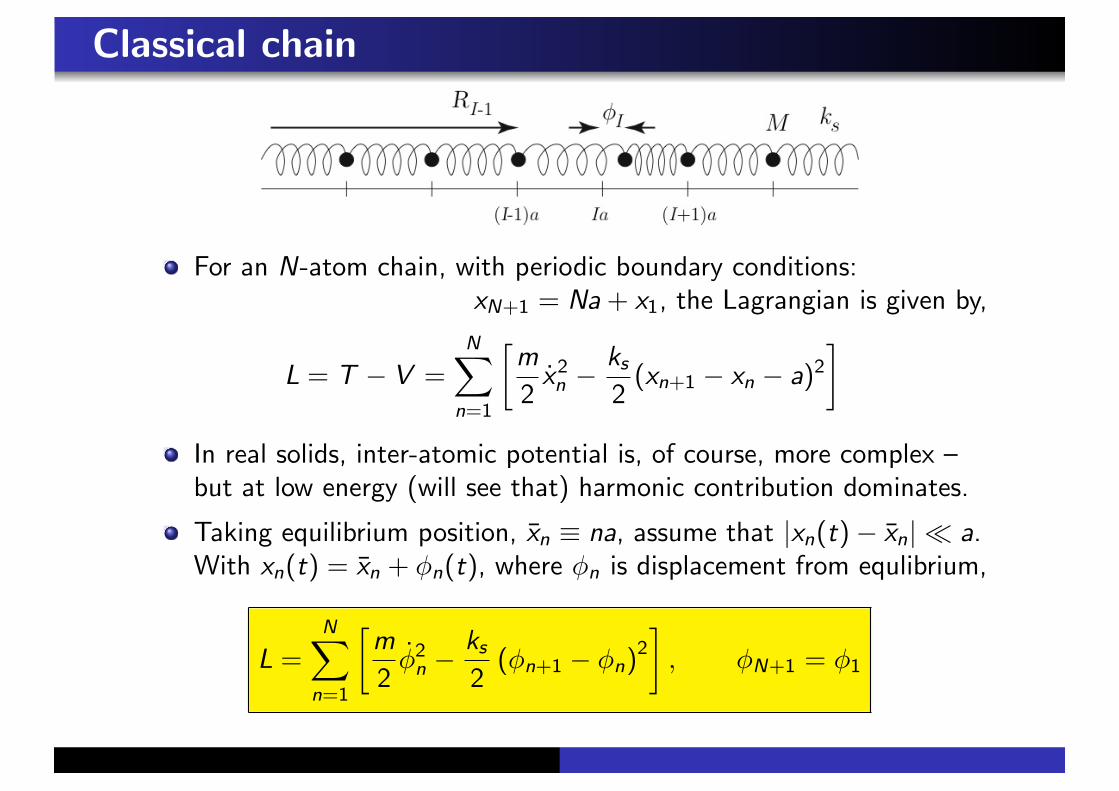
For an N-atom chain, with periodic boundary conditions:xN+1 = Na + x1, the Lagrangian is given by,

L = T ! V =N!

n=1

"m

2x2n !

ks

2(xn+1 ! xn ! a)2

#

In real solids, inter-atomic potential is, of course, more complex –but at low energy (will see that) harmonic contribution dominates.

Taking equilibrium position, xn " na, assume that |xn(t)! xn|# a.With xn(t) = xn + !n(t), where !n is displacement from equlibrium,

L =N!

n=1

"m

2!2

n !ks

2(!n+1 ! !n)

2#

, !N+1 = !1

Classical chain: equations of motion

L =N!

n=1

"m

2!2

n !ks

2(!n+1 ! !n)

2#

, !N+1 = !1

To obtain classical equations of motion from L, we can make use ofHamilton’s extremal principle:

For a point particle with coordinate x(t), the (Euler-Lagrange)equations of motion obtained from minimizing action

S [x ] =

$dt L(x , x) ! d

dt("xL)! "xL = 0

e.g. for a free particle in a harmonic oscillator potentialV (x) = 1

2kx2,

L(x , x) =1

2mx2 ! 1

2m#2x2

and Euler-Lagrange equations translate to familiar equation ofmotion, mx = !kx .

Classical chain: equations of motion

L =N!

n=1

"m

2!2

n !ks

2(!n+1 ! !n)

2#

, !N+1 = !1

Minimization of the classical action for the chain, S =%

dt L[!n, !n]leads to family of coupled Euler-Lagrange equations,

d

dt("!n

L)! "!nL = 0

With "!nL = m!n and "!nL = !ks(!n ! !n+1)! ks(!n ! !n!1), we

obtain the discrete classical equations of motion,

m!n = !ks(!n ! !n+1)! ks(!n ! !n!1) for each n

These equations describe the normal vibrational modes of thesystem. Setting !n(t) = e i"t!n, they can be written as

(!m#2 + 2ks)!n ! ks(!n+1 + !n!1) = 0

Classical chain: normal modes

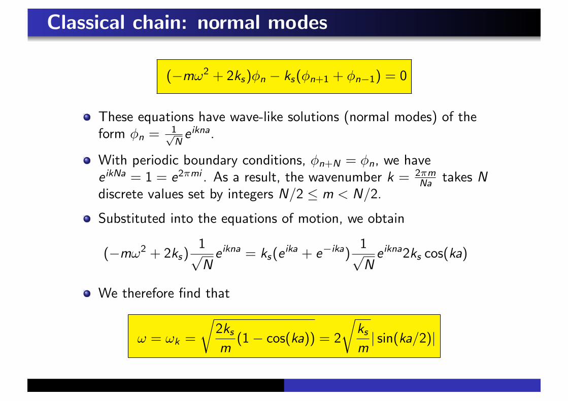
(!m#2 + 2ks)!n ! ks(!n+1 + !n!1) = 0

These equations have wave-like solutions (normal modes) of theform !n = 1"

Ne ikna.

With periodic boundary conditions, !n+N = !n, we havee ikNa = 1 = e2#mi . As a result, the wavenumber k = 2#m

Na takes Ndiscrete values set by integers N/2 $ m < N/2.

Substituted into the equations of motion, we obtain

(!m#2 + 2ks)1%N

e ikna = ks(eika + e!ika)

1%N

e ikna2ks cos(ka)

We therefore find that

# = #k =

&2ks

m(1! cos(ka)) = 2

&ks

m| sin(ka/2)|

Classical chain: normal modes

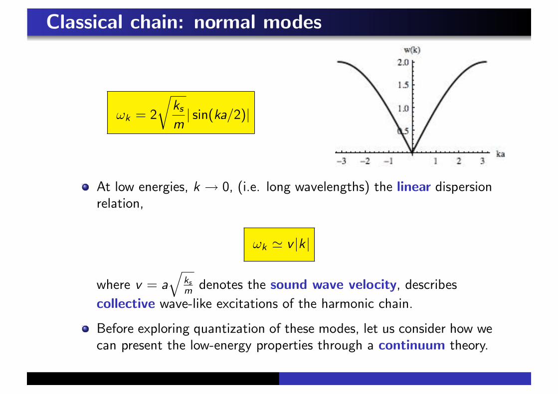
#k = 2

&ks

m| sin(ka/2)|

At low energies, k & 0, (i.e. long wavelengths) the linear dispersionrelation,

#k ' v |k|

where v = a'

ksm denotes the sound wave velocity, describes

collective wave-like excitations of the harmonic chain.

Before exploring quantization of these modes, let us consider how wecan present the low-energy properties through a continuum theory.

Classical chain: continuum limit

L =N!

n=1

"m

2!2

n !ks

2(!n+1 ! !n)

2#

For low energy dynamics, relative displacement of neighbours issmall, |!n+1 ! !n|# a, and we can transfer to a continuum limit:

!n & !(x)|x=na, !n+1 ! !n & a"x!(x)|x=na,N!

n=1

& 1

a

$ L=Na

0dx

Lagrangian L[!] =% L0 dx L(!, !), where Lagrangian density

L(!, !) =$

2!2 ! %sa2

2("x!)2

$ = m/a is mass per unit length and %s = ks/a.

Classical chain: continuum limit

L(!, !) =$

2!2 ! %sa2

2("x!)2

By turning to a continuum limit, we have succeeded in abandoningthe N-point particle description in favour of one involving a set ofcontinuous degrees of freedom, !(x) – known as a (classical) field.

Dynamics of !(x , t) specified by the Lagrangian and actionfunctional

L[!] =

$ L=Na

0dx L(!, !), S [!] =

$dt L[!]

To obtain equations of motion, we have to turn again to theprinciple of least action.

Dynamics of harmonic chain

L(!, !) =$

2!2 ! %sa2

2("x!)2

For a system with many degrees of freedom, we can still apply thesame variational principle: !(x , t)& !(x , t) + &'(x , t)

lim$#0

1

&(S [! + &']! S [!])

!= 0 =

$dt

$ L

0dx

($ !' ! %sa

2 "x!"x')

Integrating by parts

$dt

$ L

0dx($!! %sa

2"2x!)' = 0

Since this relation must hold for any function '(x , t), we must have

$!! %sa2"2

x! = 0

Dynamics of harmonic chain

L(!, !) =$

2!2 ! %sa2

2("x!)2

Classical equations of motion associated with Lagrangian densitytranslate to classical wave equation:

$!! %sa2"2

x! = 0

Solutions have the general form: !+(x + vt) + !!(x ! vt) wherev = a

*%s/$ = a

*ks/m, and !± are arbitrary smooth functions.

Low energy elementary excitations are lattice vibrations, soundwaves, propagating to left or right at constant velocity v .

Simple behaviour is consequence of simplistic definition of potential— no dissipation, etc.

Quantization of classical chain

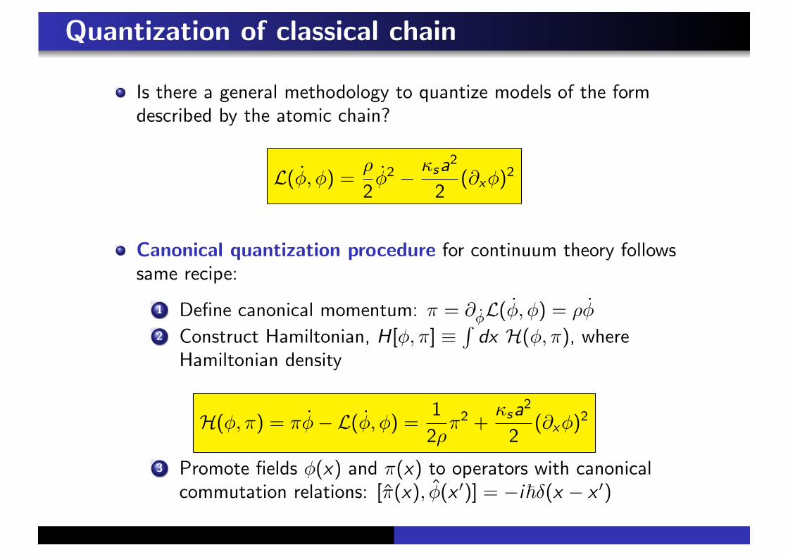
Is there a general methodology to quantize models of the formdescribed by the atomic chain?

L(!, !) =$

2!2 ! %sa2

2("x!)2

Recall the canonical quantization procedure for point particlemechanics:

1 Define canonical momentum: p = "xL(x , x)

2 Construct Hamiltonian,

H(x , p) = px ! L(x , x)

3 and, finally, promote conjugate coordinates x and p tooperators with canonical commutation relations: [p, x ] = !i!

Quantization of classical chain

Is there a general methodology to quantize models of the formdescribed by the atomic chain?

L(!, !) =$

2!2 ! %sa2

2("x!)2

Canonical quantization procedure for continuum theory followssame recipe:

1 Define canonical momentum: ( = "!L(!, !) = $!2 Construct Hamiltonian, H[!, (] "

%dx H(!, (), where

Hamiltonian density

H(!, () = (!! L(!, !) =1

2$(2 +

%sa2

2("x!)2

3 Promote fields !(x) and ((x) to operators with canonicalcommutation relations: [((x), !(x $)] = !i!)(x ! x $)

Quantization of classical chain

H =

$ L

0dx

"1

2$(2 +

%sa2

2("x !)2

#

For those uncomfortable with Lagrangian-based formulation, notethat we could have obtained the Hamiltonian density by takingcontinuum limit of discrete Hamiltonian,

H =N!

n=1

"p2

n

2m+

1

2ks(!n+1 ! !n)

2

#

and the canonical commutation relations,

[pm, !n] = !i!)mn (& [((x), !(x $)] = !i!)(x ! x $)

Quantum chain

H =

$ L

0dx

"1

2$(2 +

%sa2

2("x !)2

#

Operator-valued functions, ! and (, referred to as quantum fields.

Hamiltonian represents a formulation but not yet a solution.

To address solution, helpful to switch to Fourier representation:

+!(x)((x)

=1

L1/2

!

k

e{±ikx

+!k

(k,

+!k

(k" 1

L1/2

$ L

0dx e{%ikx

+!(x)((x)

wavevectors k = 2(m/L, m integer.

Since !(x) real, !(x) is Hermitian, and !k = !†!k (similarly for (k)

commutation relations: [(k , !k! ] = !i!)kk! (exercise)

Quantum chain

H =

$ L

0dx

"1

2$(2 +

%sa2

2("x !)2

#

In Fourier representation, !(x) = 1L1/2

,k e ikx !k ,

$ L

0dx ("!)2 =

!

k,k!

(ik!k)(ik$!k!)

)k+k!,0- ./ 01

L

$ L

0dx e i(k+k!)x=

!

k

k2!k !!k

Together with parallel relation for% L0 dx (2,

H =!

k

"1

2$(k (!k +

1

2$#2

k !k !!k

#

#k = v |k|, and v = a(%s/$)1/2 is classical sound wave velocity.

Quantum chain

H =!

k

"1

2$(k (!k +

1

2$#2

k !k !!k

#

Hamiltonian describes set of independent quantum harmonicoscillators (existence of indicies k and !k is not crucial).

Interpretation: classically, chain supports discrete set of wave-likeexcitations, each indexed by wavenumber k = 2(m/L.

In quantum picture, each of these excitations described by anoscillator Hamiltonian operator with a k-dependent frequency.

Each oscillator mode involves all N &) microscropic degrees offreedom – it is a collective excitation of the system.

Quantum harmonic oscillator: revisited

H =p2

2m+

1

2m#2x2

The quantum harmonic oscillator describes motion of a singleparticle in a harmonic confining potential. Eigenvalues form a ladderof equally spaced levels, !#(n + 1/2).

Although we can find a coordinate representation of the states,*x |n+, ladder operator formalism o!ers a second interpretation, andone that is useful to us now!

Quantum harmonic oscillator can be viewed as a simple systeminvolving many featureless fictitious particles, each of energy !#,created and annihilated by operators, a† and a.

Quantum harmonic oscillator: revisited

H =p2

2m+

1

2m#2x2

Specifically, introducing the operators,

a =

&m#

2!

1x + i

p

m#

2, a† =

&m#

2!

1x ! i

p

m#

2

which fulfil the commutation relations [a, a†] = 1, we have,

H = !#

1a†a +

1

2

2

The ground state (or vacuum), |0+ has energy E0 = !#/2 and isdefined by the condition a|0+ = 0.

Excitations |n+ have energy En = !#(n + 1/2) and are defined by

action of the raising operator, |n+ = (a†)n"

n!|0+, i.e. the “creation” of n

fictitious particles.

Quantum chain

H =!

k

"1

2$(k (!k +

1

2$#2

k !k !!k

#

Inspired by ladder operator formalism for harmonic oscillator, set

ak "&

m#k

2!

1!k +

i

m#k(!k

2, a†k "

&m#k

2!

1!!k !

i

m#k(k

2.

Ladder operators obey the commutation relations:

[ak , a†k! ] =

m#k

2!i

m#k([(!k , !!k ]! [!k , (k ]))kk! , [ak , ak! ] = [a†k , a

†k! ] = 0

Hamiltonian assumes the diagonal form

H =!

k

!#k

1a†kak +

1

2

2

Quantum chain: phonons

H =!

k

!#k

1a†kak +

1

2

2

Low energy excitations of discrete atomic chain behave as discreteparticles (even though they describe the collective motion of aninfinite number of “fundamental” degrees of freedom) describingoscillator wave-like modes.

These particle-like excitations, known as phonons, are characterisedby wavevector k and have a linear dispersion, #k = v |k|.

A generic state of the system is then given by

|{nk}+ =1*3i ni !

(a†k1)n1(a†k2

)n2 · · · |0+

Quantum chain: remarks

H =!

k

!#k

1a†kak +

1

2

2

In principle, we could now retrace our steps and express theelementary excitations, a†k |0+, in terms of the continuum fields, !(x)(or even the discrete degrees of freedom !n). But why should we?

Phonon excitations represent perfectly legitimate (bosonic) particleswhich have physical manifestations which can be measured directly.

We can regard phonons are “fundamental” and abandon microscopicdegrees of freedom as being irrelevant on low energy scales!

This heirarchy is generic, applying equally to high and low energyphysics, e.g. electrons can be regarded as elementary collectiveexcitation of a microscopic theory involving quarks, etc.

for a discussion, see Anderson’s article “More is di!erent”

Quantum chain: further remarks

H =!

k

!#k

1a†kak +

1

2

2, #k = v |k|

Universality: At low energies, whenphonon excitations involve longwavelengths (k & 0), modes becomeinsensitive to details at atomic scalejustifying our crude modelling scheme.

As k & 0, phonon excitations incurvanishingly small energy – thespectrum is said to be “massless”.

Such behaviour is in fact generic: thebreaking of a continuous symmetry (inthis case, translation) always leads tomassless collective excitations – knownas Goldstone modes.

Quantization of the harmonic chain: recap

Starting with the classical Lagrangian for a harmonic chain,

L =N!

n=1

"m

2!2

n !ks

2(!n+1 ! !n)

2#

, !N+1 = !1

we showed that the normal mode spectrum was characterised by alinear low energy dispersion, #k = v |k|, where v = a

*ks/m

denotes the classical sound wave velocity.

To prepare for our study of the quantization of the EM field, wethen turned from the discrete to the continuum formulation of theclassical Lagrangian setting L[!] =

% L0 dx L(!, !), where

L(!, !) =$

2!2 ! %sa2

2("x!)2

$ = m/a is mass per unit length and %s = ks/a.

Quantization of harmonic chain: recap

L(!, !) =$

2!2 ! %sa2

2("x!)2

From the minimisation of the classical action, S [!] =%

dt L[!], theEuler-Lagrange equations recovered the classical wave equation,

$! = %sa2"2

x!

with the solutions: !+(x + vt) + !!(x ! vt)

As expected from the discrete formulation, the low energyexcitations of the chain are lattice vibrations, sound waves,propagating to left or right at constant velocity v .

Quantization of harmonic chain: recap

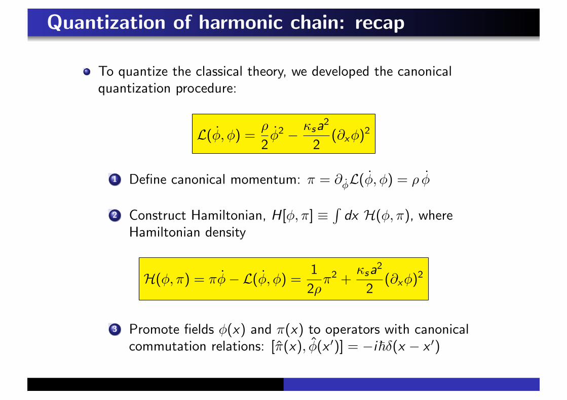
To quantize the classical theory, we developed the canonicalquantization procedure:

L(!, !) =$

2!2 ! %sa2

2("x!)2

1 Define canonical momentum: ( = "!L(!, !) = $ !

2 Construct Hamiltonian, H[!, (] "%

dx H(!, (), whereHamiltonian density

H(!, () = (!! L(!, !) =1

2$(2 +

%sa2

2("x!)2

3 Promote fields !(x) and ((x) to operators with canonicalcommutation relations: [((x), !(x $)] = !i!)(x ! x $)

Quantization of harmonic chain: recap

H =

$ L

0dx

"1

2$(2 +

%sa2

2("x !)2

#

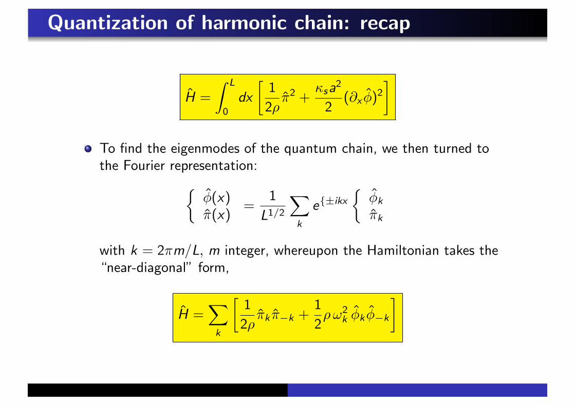
To find the eigenmodes of the quantum chain, we then turned tothe Fourier representation:

+!(x)((x)

=1

L1/2

!

k

e{±ikx

+!k

(k

with k = 2(m/L, m integer, whereupon the Hamiltonian takes the“near-diagonal” form,

H =!

k

"1

2$(k (!k +

1

2$ #2

k !k !!k

#

Quantization of harmonic chain: recap

H =!

k

"1

2$(k (!k +

1

2$ #2

k !k !!k

#

H describes set of independent oscillators with k-dependentfrequency. Each mode involves all N &) microscropic degrees offreedom – it is a collective excitation.

Inspired by ladder operator formalism, setting

ak "&

m#k

2!

1!k +

i

m#k(!k

2, a†k "

&m#k

2!

1!!k !

i

m#k(k

2.

where [ak , a†k! ] = )kk! , Hamiltonian takes diagonal form,

H =!

k

!#k

1a†kak +

1

2

2

Quantization of harmonic chain: recap

H =!

k

!#k

1a†kak +

1

2

2

Low energy excitations of discrete atomic chain behave as discreteparticles (even though they describe collective motion of an infinitenumber of “fundamental” degrees of freedom).

These particle-like excitations, known as phonons, are characterisedby wavevector k and have a linear dispersion, #k = v |k|.

A generic state of the system is then given by

|{nk}+ =1*3i ni !

(a†k1)n1(a†k2

)n2 · · · |0+

Quantization of harmonic chain: recap

H =!

k

!#k

1a†kak +

1

2

2

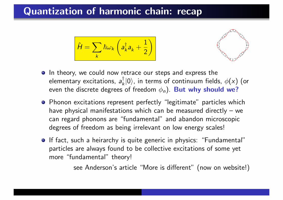
In theory, we could now retrace our steps and express theelementary excitations, a†k |0+, in terms of continuum fields, !(x) (oreven the discrete degrees of freedom !n). But why should we?

Phonon excitations represent perfectly “legitimate” particles whichhave physical manifestations which can be measured directly – wecan regard phonons are “fundamental” and abandon microscopicdegrees of freedom as being irrelevant on low energy scales!

If fact, such a heirarchy is quite generic in physics: “Fundamental”particles are always found to be collective excitations of some yetmore “fundamental” theory!

see Anderson’s article “More is di!erent” (now on website!)

Quantization of harmonic chain: second quantization

But when we studied identical quantum particles we declared that allfundamental particles can be classified as bosons or fermions – so whatabout the quantum statistics of phonons?

In fact, commutation relations tell us that phonons are bosons:

Using the relation [a†k , a†k! ] = 0, we can see that the many-body

wavefunction is symmetric under particle exchange,

|k1, k2+ = a†k1a†k2

|0+ = a†k2a†k1

|0+ = |k2, k1+

In fact, the commutation relations of the operators circumvent needto explicitly symmetrize the many-body wavefunction,

|k1, k2+ = a†k1a†k2

|0+ =1

2

(a†k1

a†k2+ a†k2

a†k1

)|0+

is already symmetrized!

Again, this property is generic and known as second quantization.

Quantization of harmonic chain: further lessons

H =!

k

!#k

1a†kak +

1

2

2, #k = v |k|

Universality: At low energies, when phononexcitations involve long wavelengths (k & 0),modes become insensitive to details at atomicscale justifying crude modelling scheme.

As k & 0, phonon excitations incurvanishingly small energy – the spectrum issaid to be “massless”.

Again, such behaviour is generic: the breakingof a continuous symmetry (in this case,translation) always leads to massless collectiveexcitations – known as Goldstone modes.

Three-dimensional lattices

Our analysis focussed on longitudinal vibrations of one-dimensionalchain. In three-dimensions, each mode associated with threepossible polarizations, *: two transverse and one longitudinal.

Taking into account all polarizations

H =!

k%

!#k%

1a†k,%ak,% +

1

2

2

where #k% = v%|k| and v% are respective sound wave velocities.

Let us apply this result to obtain internal energy and specific heatdue to phonons.

Example: Debye theory of solids

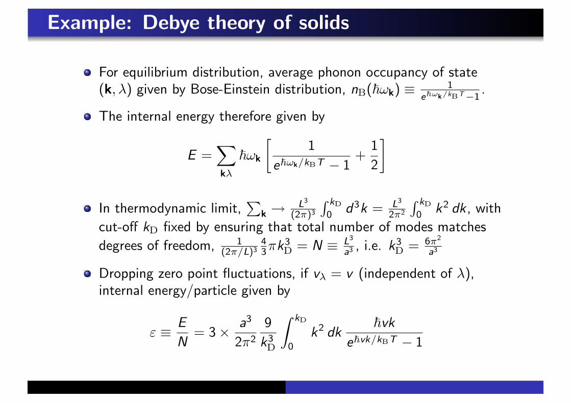
For equilibrium distribution, average phonon occupancy of state(k, *) given by Bose-Einstein distribution, nB(!#k) " 1

e!!k/kBT!1.

The internal energy therefore given by

E =!

k%

!#k

"1

e!"k/kBT ! 1+

1

2

#

In thermodynamic limit,,

k &L3

(2#)3

% kD

0 d3k = L3

2#2

% kD

0 k2 dk, withcut-o! kD fixed by ensuring that total number of modes matchesdegrees of freedom, 1

(2#/L)343(k3

D = N " L3

a3 , i.e. k3D = 6#2

a3

Dropping zero point fluctuations, if v% = v (independent of *),internal energy/particle given by

+ " E

N= 3, a3

2(2

9

k3D

$ kD

0k2 dk

!vk

e!vk/kBT ! 1

Example: Debye theory of solids

+ " E

N=

9

k3D

$ kD

0k2 dk

!vk

e!vk/kBT ! 1.

Defining Debye temperature, kBTD = !vkD,

+ = 9kBT

1T

TD

23 $ TD/T

0

z3 dz

ez ! 1

Leads to specific heat per particle,

cV = "T + = 9kB

1T

TD

23 $ TD/T

0

z4 dz

(ez ! 1)2=

+3kB T - TD

AT 3 T # TD

Example: Debye theory of solids

cV = "T + = 9kB

1T

TD

23 $ TD/T

0

z4 dz

(ez ! 1)2=

+3kB T - TD

AT 3 T # TD

Lecture 17

Quantization of theElectromagnetic Field

Quantum electrodynamics

As with harmonic chain, electromagnetic (EM) field satisfies waveequation in vacua.

1

c2E = .2E,

1

c2B = .2B

Generality of quantization procedure for chain suggests thatquantization of EM field should proceed in analogous manner.

However, gauge freedom of vector potential introduces redundantdegrees of freedom whose removal on quantum level is notcompletely straightforward.

Therefore, to keep discussion simple, we will focus on a simpleone-dimensional waveguide geometry to illustrate main principles.

Classical theory of electromagnetic field

In vacuum, Lagrangian density of EM field given by

L = ! 1

4µ0Fµ&Fµ&

where Fµ& = "µA& ! "&Aµ denotes EM field tensor, E = A iselectric field, and B = ., A is magnetic field.

In absence of current/charge sources, it is convenient to adoptCoulomb gauge, . ·A = 0, with the scalar component ! = 0, when

L[A,A] =

$d3x L =

1

2µ0

$d3x

"1

c2A2 ! (., A)2

#

Corresponding classical equations of motion lead to wave equation

1

c2A = .2A /& "µFµ& = 0

Classical theory of electromagnetic field

L[A,A] =1

2µ0

$d3x

"1

c2A2 ! (., A)2

#

Structure of Lagrangian mirrors that of harmonic chain:

L[!, !] =

$dx

"$

2!2 ! %sa2

2("x!)2

#

By analogy with chain, to quantize classical field, we should elevatefields to operators and switch to Fourier representation.

However, in contrast to chain, we are now dealing with

(i) a full three-dimensional Laplacian acting upon...

(ii) the vector field A that is...

(iii) subject to the constraint . · A = 0.

Classical theory of EM field: waveguide

L[A,A] =1

2µ0

$d3x

"1

c2A2 ! (., A)2

#

We can circumvent di"culties by considering simplifed geometrywhich reduces complexity of eigenvalue problem.

In a strongly anisotropic waveguide, the low frequency modesbecome quasi one-dimensional, specified by a single wavevector, k.

For a classical EM field, the modes of the cavity must satisfyboundary conditions commensurate with perfectly conducting walls,en , E " E&|boundary = 0 and en · B " B'|boundary = 0.

Classical theory of EM field: waveguide

For waveguide, general vector potential configuration may beexpanded in eigenmodes of classical wave equation,

!.2uk(x) = *kuk(x)

where uk are real and orthonormal,%

d3x uk · uk! = )kk! (cf. Fourier

mode expansion of !(x) and ((x)).

With boundary conditions u&|boundary = 0 (cf. E&|boundary = 0), foranisotropic waveguide with Lz < Ly # Lx , smallest *k are thosewith kz = 0, ky = (/Ly , and kx " k # L!1

z,y ,

uk =2%V

sin((y/Ly ) sin(kx) ez , *k = k2 +

1(

Ly

22

Classical theory of EM field: waveguide

L[A,A] =1

2µ0

$d3x

"1

c2A2 ! (., A)2

#

Setting A(x, t) =,

k ,k(t)uk(x), with k = (n/L and n integer,and using orthonormality of functions uk(x),

L[,,,] =1

2µ0

!

k

"1

c2,2

k ! *k,2k

#

i.e. system described in terms of independent dynamical degrees offreedom, with coordinates ,k (cf. atomic chain),

L[!, !] =

$dx

"$

2!2 ! %sa2

2("x!)2

#

Quantization of classical EM field

L[,,,] =1

2µ0

!

k

"1

c2,2

k ! *k,2k

#

1 Define canonical momenta (k = "'kL = &0,k , where &0 = 1µ0c2 is

vacuum permittivity

H =!

k

(k ,k ! L =!

k

11

2&0(2

k +1

2&0c

2*k,2k

2

2 Quantize operators: ,k & ,k and (k & (k .

3 Declare commutation relations: [(k , ,k! ] = !i!)kk! :

H =!

k

"(2

k

2&0+

1

2&0#

2k ,

2k

#, #2

k = c2*k

Quantization of classical EM field

H =!

k

"(2

k

2&0+

1

2&0#

2k ,

2k

#, #2

k = c2*k

Following analysis of atomic chain, if we introduce ladder operators,

ak =

&&0#k

2!

1,k +

i

&0#k(k

2, a†k =

&&0#k

2!

1,k !

i

&0#k(k

2

with [ak , a†k! ] = )kk! , Hamiltonian takes familiar form,

H =!

k

!#k

1a†kak +

1

2

2

For waveguide of width Ly , !#k = c[k2 + ((/Ly )2]1/2.

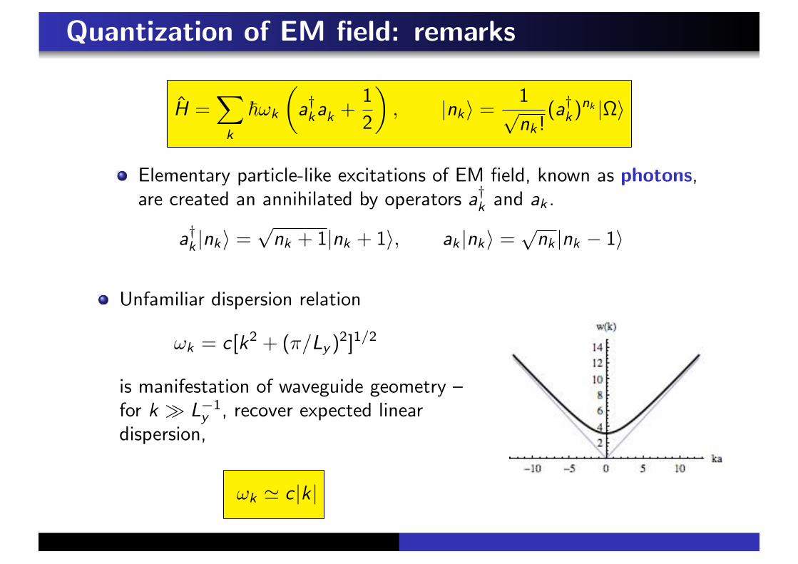
Quantization of EM field: remarks

H =!

k

!#k

1a†kak +

1

2

2, |nk+ =

1%nk !

(a†k)nk |#+

Elementary particle-like excitations of EM field, known as photons,are created an annihilated by operators a†k and ak .

a†k |nk+ =%

nk + 1|nk + 1+, ak |nk+ =%

nk |nk ! 1+

Unfamiliar dispersion relation

#k = c[k2 + ((/Ly )2]1/2

is manifestation of waveguide geometry –for k - L!1

y , recover expected lineardispersion,

#k ' c |k|

Quantization of EM field: generalization

So far, we have considered EM field quantization for a waveguide – whathappens in a three-dimensional cavity or free space?

For waveguide geometry, we have seen that A(x) =,

k ,kuk where

,k =

&!

2&0#k(ak + a†k)

In a three-dimensional cavity, vector potential can be expanded inplane wave modes as

A(x) =!

k%=1,2

&!

2&0#kV

4ek%ak%e ik·x + e(k%a†k%e!ik·x

5

where V is volume, #k = c |k|, and ek% denote two sets of (generallycomplex) normalized polarization vectors (e(k% · ek% = 1).

Quantization of EM field: generalization

A(x) =!

k%=1,2

&!

2&0#kV

4ek%ak%e ik·x + e(k%a†k%e!ik·x

5

Coulomb gauge condition, . · A = 0,requires ek% · k = e(k% · k = 0.

If vectors ek% real (in-phase), polarizationlinear, otherwise circular – typicallydefine ek% · ekµ = )µ& .

Finally, operators obey (bosonic)commutation relations,

[ak%, a†k!%! ] = )k,k!)%%!

while [ak%, ak!%! ] = 0 = [a†k%, a†k!%! ].

Quantization of EM field: generalization

A(x) =!

k%=1,2

&!

2&0#kV

4ek%ak%e ik·x + e(k%a†k%e!ik·x

5

With these definitions, the photon Hamiltonian then takes the form

H =!

k%

!#k

4a†k%ak% + 1/2

5

Defining vacuum, |#+, eigenstates involve photon number states,

|{nk%}+ =1*3k% nk%!

(a†k1%)nk1"(a†k2%

)nk2" · · · |#+

N.B. commutation relations of bosonic operators ensures thatmany-photon wavefunction symmetrical under exchange.

Momentum carried by photon field

Classical EM field carries linear momentum density, S/c2 whereS = E, B/µ0 denotes Poynting vector, i.e. total momentum

P =

$d3x

1

c2S = !&0

$d3x A(x, t), (., A(x, t))

After quantization, find (exercise)

P =!

k%

!k a†k%ak%

i.e. P|k, *+ = Pa†k,%|#+ = !k|k, *+ (for both * = 1, 2).

Angular momentum carried by photon field

Angular momentum L = x, P includes intrinsic component,

M = !$

d3x A, A (& M = !i!!

k

ek

4a†k1ak2 ! a†k2ak1

5

Defining creation operators for right/left circular polarization,

a†kR =1%2(a†k1 + ia†k2), a†kL =

1%2(a†k1 ! ia†k2)

find that

M =!

k

!ek

4a†kRakR ! a†kLakL

5

Therefore, since ek · M|k,R/L+ = ±!|k,R/L+, we conclude thatphotons carry intrinsic angular momentum ±! (known as helicity),oriented parallel/antiparallel to direction of momentum propagation.

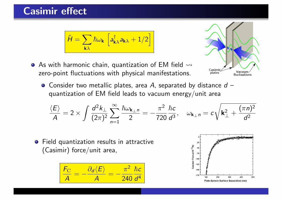
Casimir e!ect

H =!

k%

!#k

4a†k%ak% + 1/2

5

As with harmonic chain, quantization of EM field !zero-point fluctuations with physical manifestations.

Consider two metallic plates, area A, separated by distance d –quantization of EM field leads to vacuum energy/unit area

*E +A

= 2,$

d2k'(2()2

)!

n=1

!#k"n

2= ! (2

720

!c

d3, #k"n = c

&k2' +

((n)2

d2

Field quantization results in attractive(Casimir) force/unit area,

FC

A= !"d*E +

A= ! (2

240

!c

d4

Quantum field theory: summary

Starting with continuum field theory of the classical harmonic chain,

L[!, !] =

$dx

"$

2!2 ! %sa2

2("x!)2

#

we have developed a general quantization programme.

From this programme, we find that the low-energy elementaryexcitations of the chain are described by (bosonic) particle-likecollective excitations known as phonons,

H =!

k

!#k(a†kak + 1/2), !#k = v |k|

In three-dimensional system, modes acquire polarization index, *.

Quantum field theory: summary

Starting with continuum field theory of EM field for waveguide,

L[,,,] =!

k

"1

c2,2 ! *k,

2k

#

we applied quantization procedure to establish quantum theory.

These studies show that low-energy excitations of EM fielddescribed by (bosonic) particle-like modes known as photons,

H =!

k

!#k(a†kak + 1/2), #k = c(k2 + ((/Ly )

2)1/2

In three-dimensional system modes acquire polarization index, *.

H =!

k%

!#k(a†k%ak% + 1/2), #k = c |k|

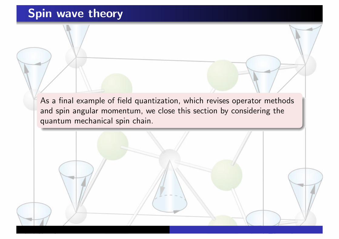
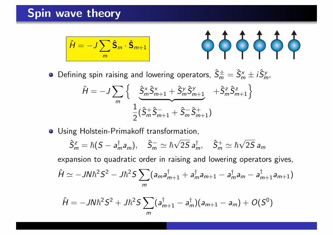
Spin wave theory

As a final example of field quantization, which revises operator methodsand spin angular momentum, we close this section by considering thequantum mechanical spin chain.

Spin wave theory

In correlated electron systems Coulomb interaction can result inelectrons becoming localized – the Mott transition.

However, in these insulating materials, the spin degrees of freedomcarried by the constituent electrons can remain mobile – suchsystems are described by quantum magnetic models,

H =!

m *=n

JmnSm · Sn

where exchange couplings Jmn denote matrix elements couplinglocal moments at lattice sites m and n.

Spin wave theory

H =!

m *=n

JmnSm · Sn

Since matrix elements Jmn decay rapidly with distance, we mayrestrict attention to just neighbouring sites, Jmn = J)m,n±1.

Although J typically positive (leading to antiferromagneticcoupling), here we consider them negative leading toferromagnetism – i.e. neighbouring spins want to lie parallel.

Consider then the 1d spin S quantum Heisenberg ferromagnet,

H = !J!

m

Sm · Sm+1

where J > 0, and spins obey spin algebra, [S'm, S(

n ] = i!)mn&'() S)m.

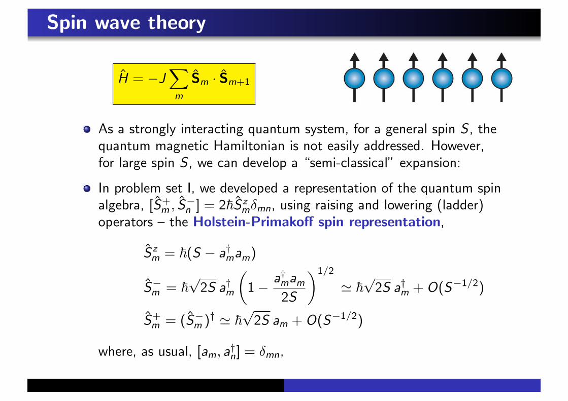
Spin wave theory

H = !J!

m

Sm · Sm+1

As a strongly interacting quantum system, for a general spin S , thequantum magnetic Hamiltonian is not easily addressed. However,for large spin S , we can develop a “semi-classical” expansion:

In problem set I, we developed a representation of the quantum spinalgebra, [S+

m , S!n ] = 2!Szm)mn, using raising and lowering (ladder)

operators – the Holstein-Primako! spin representation,

Szm = !(S ! a†mam)

S!m = !%

2S a†m

11! a†mam

2S

21/2

' !%

2S a†m + O(S!1/2)

S+m = (S!m )† ' !

%2S am + O(S!1/2)

where, as usual, [am, a†n] = )mn,

Spin wave theory

H = !J!

m

Sm · Sm+1

Defining spin raising and lowering operators, S±m = Sx

m ± i Sym,

H = !J!

m

6Sx

mSxm+1 + Sy

mSym+1/ 0- .

1

2(S+

m S!m+1 + S!m S+m+1)

+SzmSz

m+1

7

Using Holstein-Primako! transformation,

Szm = !(S ! a†mam), S!m ' !

%2S a†m, S+

m ' !%

2S am

expansion to quadratic order in raising and lowering operators gives,

H ' !JN!2S2 ! J!2S!

m

(ama†m+1 + a†mam+1 ! a†mam ! a†m+1am+1)

H = !JN!2S2 + J!2S!

m

(a†m+1 ! a†m)(am+1 ! am) + O(S0)

Spin wave theory

H = !JN!2S2 + J!2S!

m

(a†m+1 ! a†m)(am+1 ! am) + O(S0)

Taking continuum limit, am+1 ! am ' "xa(x)|x=m (unit spacing),

H = !JN!2S2 + J!2S

$ N

0dx ("xa

†)("xa) + O(S0)

As with harmonic chain, Hamiltonian can be diagonalized by Fouriertransformation. With periodic boundary conditions, a†m+N = a†m,

a(x) =1%N

!

k

e ikxak , ak =1%N

$ N

0dx e!ikxa(x)

where sum on k = 2(n/N, runs over integers n and [ak , a†k! ] = )kk! ,

$ N

0dx ("xa

†)("xa) =!

kk!

(!ika†k)(ik$ak!)

1

N

$ N

0dx e i(k!k!)x

/ 0- .)kk!

=!

k

k2a†kak

Spin wave theory

As a result, we obtain

H ' !JN!2S2 +!

k

!#ka†kak

where #k = J!Sk2 represents thedispersion of the spin excitations (cf.linear dispersion of harmonic chain).

As with harmonic chain, magneticsystem defined by massless low-energycollective excitations known as spinwaves or magnons.

Spin wave spectrum can be recordedby neutron scattering measurements.