Embed Size (px)
Citation preview

Lecture 12 CSE 260 – Parallel Computation
(Fall 2015) Scott B. Baden
Stencil methods

Announcements • Weds office hours (11/4): 3:30 to 4:30 • For remainder of quarter: 3:30 to 5:30
Scott B. Baden / CSE 260, UCSD / Fall '15 2

Today’s lecture
• Stencil methods on the GPU • Aliev Panfilov Method (A3) • CUDA Implementation
Scott B. Baden / CSE 260, UCSD / Fall '15 3

Recapping from last time
• The warp scheduler dynamically reorders instructions to avoid pipeline stalls and other hazards
• We use scoreboarding to keep track of instruction progress and available resources
• Branches serialize execution within a warp • Warp aware coding can avoid divergence
Scott B. Baden / CSE 260, UCSD / Fall '15 4

Warp aware summation
__global__ void reduce(int *input, unsigned int N, int *total){ unsigned int tid = threadIdx.x; unsigned int i = blockIdx.x * blockDim.x + tid; unsigned int s; for (s = blockDim.x/2; s > 1; s /= 2) { __syncthreads(); if (tid < s ) x[tid] += x[tid + s ]; } if (tid == 0) atomicAdd(total,x[tid]); }
reduceSum <<<N/512,512>>> (x,N)
Scott B. Baden / CSE 260, UCSD / Fall '15 5
7
11 14
25
7 0
4
3 1
5
4 1
9
6 3
For next time: complete the code so it handles global data with arbitrary N

Stencil methods
• Many physical problems are simulated on a uniform mesh in 1, 2 or 3 dimensions
• Field variables defined on a discrete set of points
• A mapping from ordered pairs to physical observables like temperature and pressure
• Important applications u Differential equations u Image processing
Scott B. Baden / CSE 260, UCSD / Fall '15 6

Motivating App: Digital Image Processing
Red
Blue
Green
x
y
RGB representation Ryan Cuprak
Photos by Martin Juell
wikipedia
Scott B. Baden / CSE 260, UCSD / Fall '15 7
• We represent the image in terms of pixels • In color image, each pixel can contain 3 colors: RGB

Image smoothing algorithm • An important operation is called image smoothing • Replace each pixel by the average of its neighbors • Repeat as many times as necessary
while not smooth enough do: for (i,j) in 0:N-1 x 0:N-1
Inew [i,j] = ( I[i-1,j] + I[i+1,j]+ I[i,j-1]+ I[i, j+1])/4 I =Inew
end while
Original 100 iter 1000 iter
Scott B. Baden / CSE 260, UCSD / Fall '15 8
i, j+1
i, j-1
i+1, j i-1, j

A motivating app from biomedical computing • Model signal propagation in cardiac tissue using the
Aliev-Panfilov method u Demonstrates complex behavior of spiral waves that are known to
cause life-threatening situations • Reaction-diffusion system of equeastions
u Reactions are the cellular exchanges of certain ions across the cell membrane during the cellular electrical impulse
• Our simulation has two state variables u Transmembrane potential: e u Recovery of the tissue: r
Scott B. Baden / CSE 260, UCSD / Fall '15 9

The Aliev-Panfilov Model • Two parts
u 2 Ordinary Differential Equations • Kinetics of reactions occurring at every point in space
u Partial Differential Equation • Spatial diffusion of reactants
• A differential equation is a set of equations involving derivatives of a function (or functions), and specifies a solution to be determined under certain constraints
• Constraints often specify boundary conditions or initial values that the solution must satisfy
Scott B. Baden / CSE 260, UCSD / Fall '15 10

Discrete approximations • The functions appearing in the differential equations
are continuous • On the computer, we can represent discrete values only • We will approximate the solution on the mesh using the
method of finite differences • We use first-order explicit numerical scheme • For example, we represent a 2nd derivative as
uʹʹ ≈ (u(x+h) – 2u(x) + u(x-h))/h2
= (u[i+1] – 2*u[i] + u[i+1])/h2
h
ui-1 ui ui+1
Scott B. Baden / CSE 260, UCSD / Fall '15 11

Computational loop of the cardiac simulator • ODE solver:
u No data dependency, trivially parallelizable u Requires a lot of registers to hold temporary variables
• PDE solver: u Jacobi update for the 5-point Laplacian operator. u Sweeps over a uniformly spaced mesh u Updates voltage to weighted contributions from
the 4 nearest neighbors updating the solution as a function of the values in the previous time step
For a specified number of iterations, using supplied initial conditions repeat for (j=1; j < m+1; j++) // PDE SOLVER for (i=1; i < n+1; i++) E[j,i] = E_p[j,i]+α*(E_p[j,i+1]+E_p[j,i-1]-4*E_p[j,i]+E_p[j+1,i]+E_p[j-1,i]); for (j=1; j < m+1; j++) // ODE SOLVER for (i=1; i < n+1; i++){ E[j,i] += -dt*(kk*E[j,i]*(E[j,i]-a)*(E[j,i]-1)+E[j,i]*R[j,i]); R[j,i] += dt*(ε+M1* R[j,i]/(E[j,i]+M2))*(-R[j,i]-kk*E[j,i]*(E[j,i]-b-1)); } swap E_p and E End repeat Scott B. Baden / CSE 260, UCSD / Fall '15 12

Performance of the simulator on Sorken • Use valgrind to obtain cache performance, down to the
source line (see Getting Started with Bang for instructions, same as for Sorken) make –j N runs parallelizes the make on N threads
• Program runs very slowly so be sure to use a qlogin node valgrind --tool=cachegrind ./apf -n 256 -i 2000 cg_annotate --auto=yes cachegrind.out.7090 > Report.txt
==7090== I refs: 4,450,799,729 ==7090== I1 misses: 2,639 I1 miss rate: 0.00% ==7090== LLi misses: 2,043 LLi miss rate: 0.00% ==7090== D refs: 1,776,861,883 (1,381,173,237 rd + 395,688,646 wr) ==7090== D1 misses: 67,387,402 ( 50,592,465 rd + 16,794,937 wr) ==7090== LLd misses: 33,166 ( 7,051 rd + 26,115 wr) ==7090== D1 miss rate: 3.7% ( 3.6% + 4.2% ) ==7090== LLd miss rate: 0.0% ( 0.0% + 0.0% ) ==7090== LL refs: 67,390,041 ( 50,595,104 rd + 16,794,937 wr) ==7090== LL misses: 35,209 ( 9,094 rd + 26,115 wr) ==7090== LL miss rate: 0.0% ( 0.0% + 0.0% )
Scott B. Baden / CSE 260, UCSD / Fall '15 14

Where is the time spent? [Provided Code] • Loops are unfused
I1 cache: 32768 B, 64 B, 8-way associativeD1 cache: 32768 B, 64 B, 8-way associativeLL cache: 20971520 B, 64 B, 20-way associativeCommand: ./apf -n 256 -i 2000-------------------------------------------------------------------------------- Ir I1mr ILmr Dr D1mr DLmr Dw D1mw DLmw4.451B 2,639 2,043 1,381,173,237 50,592,465 7,051 3957M 16,794,937 26,115 PROGRAM TOTALS Dr D1mr--------------------------------------------------------------------------------1,380,464,019 50,566,007 solve.cpp:solve( ...) . . . // Fills in the TOP Ghost Cells 10,000 1,999 for (i = 0; i < n+2; i++) 516,000 66,000 E_prev[i] = E_prev[i + (n+2)*2]; // Fills in the RIGHT Ghost Cells 10,000 0 for i = (n+1); i < (m+2)*(n+2); i+=(m+2)) 516,000 504,003 E_prev[i] = E_prev[i-2]; // Solve for the excitation, a PDE 1,064,000 8,000 for(j =innerBlkRowStartIndx;j<=innerBlkRowEndIndx; j+=(m+)){
0 0 E_prevj = E_prev + j; E_tmp = E + j; 512,000 0 for(i = 0; i < n; i++) {721,408,002 16,630,001 E_tmp[i] = E_prevj[i]+alpha*(E_prevj[i+1]...) } // Solve the ODEs 4,000 4,000 for(j=innerBlkRowStartIndx; j <= innerBlkRowEndIndx;j+=(m+3)){ for(i = 0; i <= n; i++) { 262,144,000 33,028,000 E_tmp[i] += -dt*(kk*E_tmp[i]*(E_tmp[i]-a).. )*R_tmp[i]); 393,216,000 4,000 R_tmp[i] += dt*(ε+M1*R_tmp[i]/(E_tmp[i]+M2))*(…); }
Scott B. Baden / CSE 260, UCSD / Fall '15 15

Fusing the loops • Slows down the simulation by 20% • # data references drops by 35%, total number of read misses
drops by 48% • What happened?
Scott B. Baden / CSE 260, UCSD / Fall '15 16
For a specified number of iterations, using supplied initial conditions repeat for (j=1; j < m+1; j++){ for (i=1; i < n+1; i++) { // PDE SOLVER E[j,i] = E_p[j,i]+α*(E_p[j,i+1]+E_p[j,i-1]-4*E_p[j,i]+E_p[j+1,i]+E_p[j-1,i]); // ODE SOLVER E[j,i] += -dt*(kk*E[j,i]*(E[j,i]-a)*(E[j,i]-1)+E[j,i]*R[j,i]); R[j,i] += dt*(ε+M1* R[j,i]/(E[j,i]+M2))*(-R[j,i]-kk*E[j,i]*(E[j,i]-b-1)); } } swap E_p and E End repeat

Today’s lecture
• Stencil methods on the GPU • Aliev Panfilov Method (A3) • CUDA Implementation
Scott B. Baden / CSE 260, UCSD / Fall '15 18

Naïve CUDA Implementation • All array references go through device memory
for (j=1; j<= m+1; j++) for (i=1; i<= n+1; i++) E[j][i] = E′ [j][i]+α*(E′ [j][i-1]+E′ [j][i+1] + E′ [j-1][i]+E′ [j+1][i] - 4*E′ [j][i]);
#define E′ [i,j] E_prev[j*(m+2) + i]
J = blockIdx.y*blockDim.y + threadIdx.y; I = blockIdx.x*blockDim.x + threadIdx.x; if ((I > 0) && (I <= n) && (J > 0) && (J <= m) ) E[I] = E′ [I,J] + α*(E′ [I-1,J] + E′ [I+1,J] + E′ [I,J-1]+ E′ [I,J+1] – 4*E′ [I,J]);
Scott B. Baden / CSE 260, UCSD / Fall '15 19
P0 P1 P2 P3
P4
P8
P12
P5 P6 P7
P9 P11
P13 P14
P10
n
n np
np
P15

Nx
Ny
Cuda thread block
dx
dy
Using Shared Memory (Device Cap 3.5, 3.7 &1.3)
Didem Unat
Scott B. Baden / CSE 260, UCSD / Fall '15 21
PDE Part Et[i,j] = Et-1[i,j] + α(Et-1[i+1,j] + Et-1[i-1,j] + Et-1[i,j+1] + Et-1[i,j-1] - 4Et-1[i,j])

Handling Ghost Cells • Two approaches
u Assign 1 thread to each mesh cell including ghost cells u Assign 1 thread to interior cells only
• Divide work between threads so each thread responsible for one ghost cell load
• Thread divergence, but cost differs • For 16 × 16 tile size: 16×4 - 4 = 60 ghost cells
Ghost cells Each thread loads one ghost cell Thread uses a hash map to find its ghost cell assignment
Scott B. Baden / CSE 260, UCSD / Fall '15 23
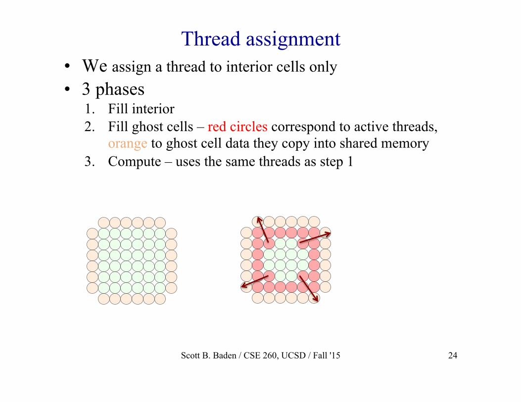
Thread assignment • We assign a thread to interior cells only • 3 phases
1. Fill interior 2. Fill ghost cells – red circles correspond to active threads,
orange to ghost cell data they copy into shared memory 3. Compute – uses the same threads as step 1
Scott B. Baden / CSE 260, UCSD / Fall '15 24

CUDA Code to load shared memory
__shared__ float block[DIM_Y + 2 ][DIM_X + 2 ]; int idx = threadIdx.x, idy = threadIdx.y; //local indices //global indices int x = blockIdx.x * (DIM_X) + idx; int y = blockIdx.y * (DIM_Y) + idy; idy++; idx++; // Why do we increment? unsigned int index = y * N + x ; //interior points float center = E_prev[index] ; // Where is center stored? block[idy][idx] = center; __syncthreads();
Scott B. Baden / CSE 260, UCSD / Fall '15 25

Copying the ghost cells
Didem Unat
if (idy == 1 && y > 0 ) block[0][idx]= E_prev[index - N]; else if(idy == DIM_Y && y < N-1) block[DIM_Y+1][idx] = E_prev[index + N]; if ( idx==1 && x > 0 ) block[idy][0] = E_prev[index - 1]; else if( idx== DIM_X && x < N-1 ) block[idy][DIM_X +1] = E_prev[index + 1]; __syncthreads();
1 thread for each interior cell
Scott B. Baden / CSE 260, UCSD / Fall '15 26

The stencil computation and ODE float r = R[index]; float e = center + α* ( block[idy][idx-1] + block[idy][idx+1] + block[idy-1][idx] + block[idy+1][idx] - 4*center); e = e - dt*(kk * e * ( e- a) * ( e - 1 ) + e * r); E[index] = e; R[index] = r + dt *(ε+ M1 * r / ( e + M2 ) ) * ( -r - kk * e * (e - b - 1));
Scott B. Baden / CSE 260, UCSD / Fall '15 27

Top Row in Registers Curr Row in Shared memory Bottom Row in Registers
• Instead of using a 2D block of memory, we only keep 1 row in shared memory, the rest in registers
• Sliding rows with 1D thread blocks reduces global memory accesses.
Top row ← Current row, Current row ← Bottom row Bottom row ← read new row from global memory
Sliding rows scheme
…
Read new row from global memory Scott B. Baden / CSE 260, UCSD / Fall '15 28
Inter-thread communication • Historically, GPUs supported intra-block
communication via shared memory, and inter-block via global memory
• Shared memory and registers do not persist across kernel invocations
• Kepler (CC 3.0+) supports high speed atomics in global memory, that are suitable for inner loops (e.g. summation)
• New instructions support direct data exchange between threads in the same warp
• A thread can read values stored in a register from a thread within the same warp • Shift
• See http://blog.csdn.net/u010060391/article/details/21558557 http://on-demand.gputechconf.com/gtc/2013/presentations/S3174-Kepler-Shuffle-Tips-Tricks.pdf
Scott B. Baden / CSE 260, UCSD / Fall '15 30