CSE 260 Project Report

Parallelizing Pre-conditioned

Conjugate Gradient Method

with OpenMP, MPI and CUDA

12/4/2009

The Conjugate Gradient Method

Vasileios Kontorinis

Nikolaos Trogkanis

(group of 2)

Introduction The Conjugate Gradient (CG) Method is one of the most widely used iterative methods for solving sys-

tems of linear equations. CG is effective for solving systems of the form Ax = b, where x is an unknown

vector, b is a known vector and A is a known, square, symmetric, positive-definite matrix. Iterative me-

thods like CG are better when A is sparse (most of its elements are zero). When A is dense a more effi-

cient method is to factor A (e.g. with Gaussian elimination) and solve the equations with backsubstitu-

tion. Factorization takes similar time with the iterative process and CG on a sparse matrix requires a

much smaller memory footprint [1]. The reason for the latter is that the time and space complexity of

CG does not depend on the size of the array A but on the number of its non-zero elements.

The method proceeds by generating successive approximations to the solution, residuals corresponding

to the approximations, and search directions used in updating approximations and residuals.

The pseudocode for the CG algorithm is given below:

//

//

// Initializations

//

//

// Check if max iterations reached or residuals small enough

// Approximate new solution

// Estimate new residuals

// Find new direction

Where x is the solution vector, r the residuals, s the direction move next, i the number of iterations and

α, β scalars to achieve orthogonality conditions.

There is a way to speed up the convergence of conjugate gradient by solving the system M-1Ax= M-1b

instead of Ax = b. The array M-1 is chosen so that M-1A has a smaller condition number. Since the rate of

convergence degrades as the condition number of the matrix increases, the equivalent system con-

verges faster. However, finding the proper array M is not trivial. Ideally we would like M = A -1, but this is

equivalent to solving the system. We use two different arrays M for the preconditioning, the simple Ja-

cobi preconditioner and the block Jacobi preconditioner.

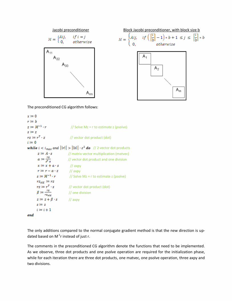
Jacobi preconditioner Block Jacobi preconditioner, with block size b

The preconditioned CG algorithm follows:

// Solve Mz = r to estimate z (psolve)

// vector dot product (dot)

// 2 vector dot products

// matrix vector multiplication (matvec)

// vector dot product and one division

// axpy

// axpy

// Solve Mz = r to estimate z (psolve)

// vector dot product (dot)

// one division

// axpy

The only additions compared to the normal conjugate gradient method is that the new direction is up-

dated based on M-1r instead of just r.

The comments in the preconditioned CG algorithm denote the functions that need to be implemented.

As we observe, three dot products and one psolve operation are required for the initialization phase,

while for each iteration there are three dot products, one matvec, one psolve operation, three axpy and

two divisions.

The total floating operations for the Jacobi preconditioned conjugate gradient method are:

Flops = Initialization computation +#iter * computation per iteration

= 3 *dot_product_flops + 1*psolve_flops + #iter * (3*dot_product_flops + 1*matvec_flops+

1*psolve_flops + 3 * axpy_flops + 2)

Assuming we employ the compressed sparse matrix row format (CSR) for the storage of A and the sim-

ple Jacobi preconditioner, it is:

Flops =3* 2*N + N + #iter * (3 * 2 * N + 2 * #elements of sparse A + N + 3 * 2 * N + 2)

We need to mention that the estimation of M-1 requires N floating point divisions. However, since divi-

sion is usually costly and these values remain constant, we assume that those are estimated once and

stored for use in the later iterations.

Assuming the block Jacobi preconditioner with a block size b we solve Mz = r for z, using Cholesky facto-

rization for each of the N/b blocks. Actually, since A is positive definite so are its diagonal blocks. Hence,

the factorization is done at the very beginning and the blocks are stored in their factored form sine M

does not change.

Flops =3 * 2*N + 2*N/b *b*b + #iter * (3 * 2N + 2 * #elements of sparse A + 2*N/b *b*b + 3 * 2 * N + 2)

Implementation Details Detailed profiling demonstrated that we should focus on the aforementioned functions: dot, axpy,

psolve and matvec. In this section we detail design decisions regarding the workload distribution for

each function across the three different technologies employed OpenMP, MPI, CUDA and present our

implementation approach.

Workload Distribution In this section we show how we distribute the workload in order to balance the work among threads for

the OpenMP framework, processes for the MPI technology and threads or warps for the CUDA technol-

ogy.

Figure 1 demonstrates how each thread or process for the OpenMP and MPI technology respectively is

responsible to operate on a stripe of the array A and the vectors x, b. The width of each stripe is deter-

mined by the size of the array A and the number of threads/processes. This partitioning involves the ma-

trix-vector multiplication, the saxpy operations as well as the dot products. What is most interesting in

this horizontal partitioning is that parts of the solution x must be broadcasted at the end of each itera-

tion. The latter significantly increases the communication overhead, to the extent that becomes the ma-

jor execution time component.

The vector x must be communicated among the nodes though either shared memory or message pass-

ing for the calculation to take place, while the stripes of A and b are stored locally.

Figure 1 Workload distribution for OpenMP and MPI

Figure 2 depicts the workload distribution in CUDA. The arrays are partitioned again in stripes but at a

much finer granularity. In CUDA we implemented two different kernels. In the first, each thread iterates

over the elements of a row. In the second, one WARP (32 threads) iterates over one row. Each tech-

nique has advantages and disadvantages. Those are discussed in the results section.

Figure 2 Workload distribution for CUDA

Implementation

1) Vector dot product (dot) OpenMP MPI CUDA

#pragma omp parallel for private(i)

reduction(+:sum)

for (i = 0; i < n; ++i)

sum += x[i] * y[i];

for (i = 0; i < n; ++i) loca_sum += x[i] * y[i]; MPI_Allreduce(&local_sum, &sum, 1,

MPI_FLOAT, MPI_SUM,

MPI_COMM_WORLD);

cublasSdot(n, x, 1, y, 1);

Vector dot product requires that the result of the multiplications is communicated to be summed up. In

OpenMP this is achieved with the reduction(+:sum) directive while in the MPI with the MPI_Allreduce

call. In CUDA we use the corresponding function from the cublas library.

2) Axpy OpenMP MPI CUDA

#pragma omp parallel for private(i)

for (i = 0; i < n; ++i)

y[i] += alpha * x[i];

for (i = 0; i < n; ++i) y[i] += alpha * x[i];

cublasSaxpy(n, alpha, x, 1, y, 1);

Axpy does not require the communication of any data among threads/processes. Therefore in OpenMP

we just denote the for loop as parallel while the MPI code is the same as the serial version. Again we use

the Saxpy from cublas library in the CUDA implementation.

3) Psolve (r= M-1x estimation) OpenMP MPI CUDA

// Jacobi preconditioner

// M = diag A , M-1 = 1/ Mij , for i = j

#pragma omp parallel for private(i)

for (i = 0; i < n; ++i)

y[i] = M-1[i] * x[i];

// Block-Jacobi preconditioner

#pragma omp parallel for

for each block

cholesky_solve(...);

// Jacobi preconditioner

// M = diag A , M-1 = 1/ Mij , for i = j for (i = 0; i < n; ++i) y[i] = M-1[i] * x[i]; // Block-Jacobi preconditioner

for each block

cholesky_solve(...);

// GPU kernel: one thread per element vecvec_kernel(…) , i = ((blockDim.x * (blockIdx.x + blockIdx.y * gridDim.x) + threadIdx.x)); if (i < n)

y[i] = M-1[i] * x[i]; } vecvec_kernel<<<grid, BLOCK_SIZE>>>(n, x, M, y); // Block-Jacobi preconditioner

for each block

cublasStrsm(...); cublasStrsm(...);

We consider the simple Jacobi preconditioner and the block Jacobi preconditioner. For the former the

estimation of r = M-1x is straightforward since the estimation of M-1 can be done once at the very begin-

ning by inversing the diagonal elements of A and then simply doing a vector-vector multiplication. How-

ever, psolve is more involved for the block-Jacobi preconditioner. Since A is positive definite, so are its

diagonal blocks. Hence we can Cholesky factor them in advance. This allows us to estimate r by Cholesky

solving Mkrk=xk for each block Mk. (In general the Cholesky method solves A*X = B where A = UT*U by

first solving UT*Y = B and then solving U*X=Y). In Cuda we use for the Cholesky solve the cublasStrsm

function from the cublas library.

4) Matrix vector multiplication (matvec) OpenMP MPI CUDA

#pragma omp parallel for private(i, j,

sum)

for (i = 0; i < n; ++i) {

sum = 0;

for (j = Arow[i]; j < Arow[i + 1]; ++j) {

sum += Aval[j] * x[Acol[j]];

}

Ax[i] = sum;

}

// Gather distributed x to x_global MPI_Allgatherv(x, n, MPI_FLOAT, x_global, A->row_counts, A->row_displs, MPI_FLOAT, MPI_COMM_WORLD); for (i = 0; i < n; ++i) { sum = 0; for (j = Arow[i]; j < Arow[i + 1]; ++j) { sum += Aval[j] * x_global[Acol[j]]; } Ax[i] = sum; }

// GPU kernel: one thread per row i = ((blockDim.x * (blockIdx.x + block-Idx.y * gridDim.x) + threadIdx.x)); if (i < n) { sum = 0; for (j = Arow[i]; j < Arow[i + 1]; ++j) sum += Aval[j] * x[Acol[j]]; Ax[i] = sum; }

The matrix vector multiplication implementation depends on the matrix storage format employed. We

use Compressed Sparse Row (CSR) format. For further details see [2]. In OpenMP x is declared as a glob-

al variable and therefore changes to it with the threads are immediately visible to other threads. How-

ever, in MPI we need to ensure that the vector x is being updated with the modifications of other

processes at the beginning of every iteration. This happens with the MPI_Allgatherv call. In CUDA we

first implemented a straightforward approach based on the CPU version where we parallelized the outer

most loop and assigned one thread per row.

Optimizations

MPI

In MPI as the number of processes scales the limiting factor for performance scaling is the communica-

tion of the solution x among processes. Therefore we consider 3 alternatives when it comes to how this

communication takes place.

c0) MPI_Allgatherv: All the processes send their local vectors x and all the processes gather them in

their x_global vector. In order to do this we need two arrays of length P (=number of processes):

row_counts[] that contains the number of elements that are received from each process, and

row_displs[] that contains the displacements at which to place the incoming data from each

process.

c1) MPI_Send and MPI_Recv only the parts of x that each process needs. In the multiplication a

process needs only those x[k] for which it has at least one non zero A[i][k] for any i.

Apparently this is expected to be an improvement over c0) since the bytes to be transmitted is

smaller. In order to do this we need to keep in a PxP array which k’s (indices of x) each process

needs from each other process. In our implementation we have the array needs[i][j] where the

entry [i,j] specifies the range of indices of x the process i needs from the process j. Note that we

do not send/receive individual x*k+’s, but we group them together to limit the number of mes-

sages and avoid the overhead of the MPI message layer.

Additionally, we have to be careful of how we order the send/receives in order to avoid dead-

locks. This is why we implemented a special communication policy that avoids deadlocks. First, a

process Pj waits to receive messages from Pi with lower rank (i<j), then, it sends messages to all

processes Pi that need something from Pj, and lastly, the process Pj waits to receive messages

from Pi with highr rank (i>j). The code used is the following: // for each process i with lower rank than the current process

for (i = 0; i < rank; ++i) {

r = needs[rank][i];

// if there are parts that the current process needs from process

i, receive them

if (r.count > 0) {

MPI_Recv(&x_global[r.start], r.count, MPI_MYFLOAT, i, 0,

MPI_COMM_WORLD, &status);

}

}

// for each process i

for (i = 0; i < nprocs; ++i) {

r = needs[i][rank];

// if process i is this process then memory copy from x to x_global

if (i == rank) {

memcpy(&x_global[r.start], &x[r.start - displ], r.count * si-

zeof(FLOAT));

} else {

// if there are parts that the process i needs from this

process, send them

if (r.count > 0) {

if (non_blocking_sends) {

MPI_Isend(&x[r.start - displ], r.count, MPI_MYFLOAT, i,

0, MPI_COMM_WORLD, &request);

} else {

MPI_Send(&x[r.start - displ], r.count, MPI_MYFLOAT, i,

0, MPI_COMM_WORLD);

}

}

}

}

// for each process with higher rank than the current process

for (i = rank + 1; i < nprocs; ++i) {

r = needs[rank][i];

// if there are parts that the current process needs from process i

receive them

if (r.count > 0) {

MPI_Recv(&x_global[r.start], r.count, MPI_MYFLOAT, i, 0,

MPI_COMM_WORLD, &status);

}

}

c2) MPI_lsend. This is non-blocking sends, where the sender can proceed without having to wait for

the full transaction to be completed. However, since communication is needed at each step

there is an implicit barrier between the processes. This implicit barrier mostly appears in the

vector dot product where communication is needed after each process has computed its local

vector dot product and for which we cannot use non-blocking sends. This is why in our experi-

ments we did not see any improvement using non-blocking sends just in the matrix vector mul-

tiplication.

We also consider 2 alternatives when it comes to how the workload is distributed.

d0) The rows are distributed evenly across processes. As described in Figure 1 each process takes on

average N/P rows. Note that the remainder N%P is distributed evenly to the first N%P processes,

each one of them takes one extra row.

d1) The number of non-zero elements is distributed evenly across processes. There might be cases

that some stripes of A in the Figure 1 contain more non-zero elements than other stripes. This

leads to load imbalance in the matrix vector multiplication since processes responsible for those

stripes will have to perform more work than the rest. This is why we implemented another dis-

tribution mode where each stripe in Figure 1 has approximately NZ/P non-zero elements, where

NZ is the total number of the non-zero elements in A. Note, however, that this workload distri-

bution now introduces load imbalance in all the other 3 methods: dot, axpy, and psolve that re-

quire evenly distribution of rows in order to be load balanced.

CUDA

In CUDA, first we noticed that the vector x in the matrix vector multiplication kernel is used many times

hence its access can easily be optimized by accessing it through the texture memory. Note that there is a

limitation that the texture cannot be floats of double precision. However, we managed to overcome this

limitation by using a texture of int2’s. In this case we fist use int2 v = tex1Dfetch(tex_x, i) to fetch an int2

from the texture and then convert the int2 to double with the help of __hiloint2double(v.y, v.x).

Second, we noticed that the biggest bottleneck was the uncoalesced memory accesses of the Aval and

Arow vectors of the sparse matrix representation. This is why we implemented a second kernel that

achieves memory coalescing by assigning a whole set of 32 threads (warp) to each row in the matrix.

However, this also means that if the average number of non-zero elements per row is not sufficient

enough there will be idle threads. In this implementation we also use shared memory to store the com-

puted local sums for each thread and at the end of the kernel the local sums are reduced to the row

sum. Note that for this reduction no synchronization is needed since threads in the same warp are guar-

anteed to be synchronized. However, this is not true for the emulator where we learned the hard way

that after each time we update the shared memory in the final sum reduction stage a call to

__syncthreads() is needed!

Results In order to explore how our optimizations behave on diverse matrices with different characteristics we

present results on three different datasets.

The first dataset is the bcsstk17 matrix downloaded from http://math.nist.gov/MatrixMarket/. This ma-

trix is 10,974 x 10,974 with 219,812 non-zero elements. The second dataset is the thermal2 matrix, by

the Schmid group downloaded from http://www.cise.ufl.edu/research/sparse/matrices/. This matrix is

1,228,045 x 1,228,045 with 8,580,313 non-zero elements. The third dataset is the bone0103D, by the

Oberwolfach group from the same source as the previous dataset. This matrix is 986,703 x 986,703 with

71,666,325 non-zero elements.

All of these datasets where selected so that A is a sparse, symmetric, real, positive-definite matrix. In

terms of their specific characteristics bcsttk17 is a relatively small array, evenly distributed, across the

diagonal. Thermal2 is a lot larger and contains elements that are not evenly distributed per row. Hence

we expect the second workload distribution mode described earlier to perform better. Finally, bone010

is the denser among the three datasets, as a result it should provide more computational workload and

performance should scale better with increasing number of threads/processes.

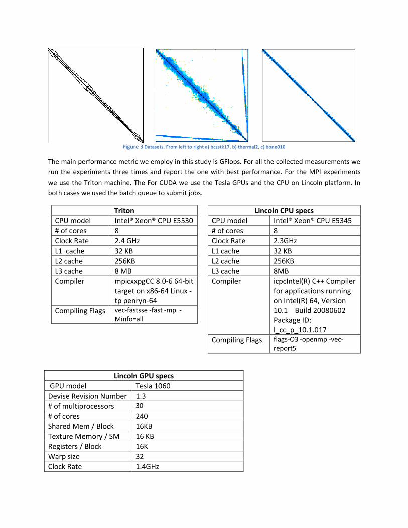
Figure 3 Datasets. From left to right a) bcsstk17, b) thermal2, c) bone010

The main performance metric we employ in this study is GFlops. For all the collected measurements we

run the experiments three times and report the one with best performance. For the MPI experiments

we use the Triton machine. The For CUDA we use the Tesla GPUs and the CPU on Lincoln platform. In

both cases we used the batch queue to submit jobs.

Triton

CPU model Intel® Xeon® CPU E5530

# of cores 8

Clock Rate 2.4 GHz

L1 cache 32 KB

L2 cache 256KB

L3 cache 8 MB

Compiler mpicxxpgCC 8.0-6 64-bit target on x86-64 Linux -tp penryn-64

Compiling Flags vec-fastsse -fast -mp -Minfo=all

Lincoln CPU specs

CPU model Intel® Xeon® CPU E5345

# of cores 8

Clock Rate 2.3GHz

L1 cache 32 KB

L2 cache 256KB

L3 cache 8MB

Compiler icpcIntel(R) C++ Compiler for applications running on Intel(R) 64, Version 10.1 Build 20080602 Package ID: l_cc_p_10.1.017

Compiling Flags flags-O3 -openmp -vec-report5

Lincoln GPU specs

GPU model Tesla 1060

Devise Revision Number 1.3

# of multiprocessors 30

# of cores 240

Shared Mem / Block 16KB

Texture Memory / SM 16 KB

Registers / Block 16K

Warp size 32

Clock Rate 1.4GHz

Compiler nvcc

Compiling Flags -c -arch=sm_13 --compiler-options -fno-strict-aliasing -O3

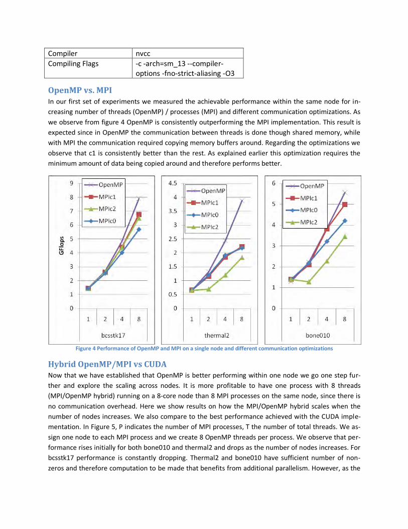
OpenMP vs. MPI In our first set of experiments we measured the achievable performance within the same node for in-

creasing number of threads (OpenMP) / processes (MPI) and different communication optimizations. As

we observe from figure 4 OpenMP is consistently outperforming the MPI implementation. This result is

expected since in OpenMP the communication between threads is done though shared memory, while

with MPI the communication required copying memory buffers around. Regarding the optimizations we

observe that c1 is consistently better than the rest. As explained earlier this optimization requires the

minimum amount of data being copied around and therefore performs better.

Figure 4 Performance of OpenMP and MPI on a single node and different communication optimizations

Hybrid OpenMP/MPI vs CUDA Now that we have established that OpenMP is better performing within one node we go one step fur-

ther and explore the scaling across nodes. It is more profitable to have one process with 8 threads

(MPI/OpenMP hybrid) running on a 8-core node than 8 MPI processes on the same node, since there is

no communication overhead. Here we show results on how the MPI/OpenMP hybrid scales when the

number of nodes increases. We also compare to the best performance achieved with the CUDA imple-

mentation. In Figure 5, P indicates the number of MPI processes, T the number of total threads. We as-

sign one node to each MPI process and we create 8 OpenMP threads per process. We observe that per-

formance rises initially for both bone010 and thermal2 and drops as the number of nodes increases. For

bcsstk17 performance is constantly dropping. Thermal2 and bone010 have sufficient number of non-

zeros and therefore computation to be made that benefits from additional parallelism. However, as the

number of nodes increases the communication costs increase as well, hence the slowdown. Bcsstk17

does not have sufficient non-zero elements to keep the CPUs occupied and therefore starts slowing

down from the very beginning. We should note that the results of the MPI/OpenMP hybrid shown in

the graph are the best among all the optimization we applied and run on Triton.

Figure 5 Performance of hybrid MPI/OpenMP on Triton when scaling number of nodes P. Comparison with GPU on Lincoln.

MPI in-depth analysis In order to understand the reasons for the poor scaling when the number of nodes/threads for the hybr-

id increases we conducted some additional experiments. The timing spent in each function can be attri-

buted to three different types. Computation is the time spent computing results. Communication is the

time spent communicating intermediate results to other processes. Synchronization is the time a

process spends waiting for other processes to reach the same execution point so that they can proceed.

These points are the communication points at MPI_Allgatherv in the beginning of the matrix-vector mul-

tiplication and the MPI_Allreduce at the end of the vector dot product. Since we wanted to measure this

synchronization time separately from the actual communication time, we explicitly added a barrier be-

fore these two communications. The synchronization time can be also seen as the time a process was

idle, hence a high value indicates load imbalance.

Figure 6 reports the worst values (maximum values) of the above times among all processes. The figure

reinforces our intuition that communication overhead is the reason for the performance degradation.

Specifically communication overhead exists for dot and matvec, with the latter being the most dominant

factor. Bones010 matrix is denser therefore benefits a lot by dividing the blue portion of computation to

multiple nodes. Furthermore, we observe that the optimization d1 that assigns rows to each process so

that the number of non-zero elements is approximately the same achieves to reduce the synchroniza-

tion time for matvec. However, because of the now uneven row partitioning the synchronization cost in

dot increases. There are now processes that own fewer rows than others, hence they finish their local

vector dot product computation faster and hence remain idle till the communication in MPI_Allreduce.

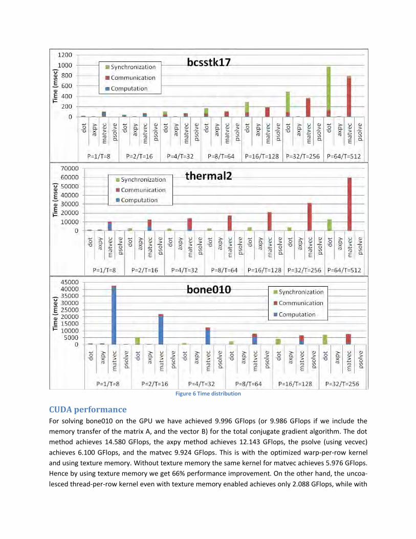
Figure 6 Time distribution

CUDA performance For solving bone010 on the GPU we have achieved 9.996 GFlops (or 9.986 GFlops if we include the

memory transfer of the matrix A, and the vector B) for the total conjugate gradient algorithm. The dot

method achieves 14.580 GFlops, the axpy method achieves 12.143 GFlops, the psolve (using vecvec)

achieves 6.100 GFlops, and the matvec 9.924 GFlops. This is with the optimized warp-per-row kernel

and using texture memory. Without texture memory the same kernel for matvec achieves 5.976 GFlops.

Hence by using texture memory we get 66% performance improvement. On the other hand, the uncoa-

lesced thread-per-row kernel even with texture memory enabled achieves only 2.088 GFlops, while with

texture memory disabled it achieves 1.923 GFlops. This means that our improved optimized kernel is

5.2x times better than the straightforward one. On Lincoln the multithreaded CPU version with 8

threads achieves 1.543 GFlops for the total conjugate gradient algorithm (4.065 GFlops for the dot,

3.388 GFlops for the axpy, 1.455 GFlops for the psolve, and 1.472 GFlops for the matvec). Therefore, our

GPU version has a 6.5x total speedup including transfer time over the 8-threaded CPU version on Lin-

coln. More specifically both the cublas function we used: cublasSdot and cublasSaxpy have 3.6x speedup

over the 8-threaded CPU version while our kernels vecvec and matvec have 4.2x and 6.8x, respectively.

The previous results, like all the other ones reported in this report, are for single precision. For double

precision solving bone010 on the GPU we achieve total 7.253 GFlops (8.765 for the dot, 6.601 for the

axpy, 3.328 for the psolve, and 7.375 for the matvec). This means that on average there is only a 27%

drop when we increase the precision from single to double on the GPU. On the other hand, on the CPU

there is only a 36% drop since the total algorithm using 8 threads achieves 0.991 GFlops (1.864 for the

dot, 1.132 for the axpy, 0.412 for the psolve and 0.977 for the matvec). Hence for double precision our

GPU version has 7.3x total speedup over the 8-threaded CPU version on Lincoln and our kernels vecvec

and matvec have a speedup of 8.1x and 7.5x, respectively.

CUDA in depth analysis To further investigate the potential performance speedups with the CUDA implementation we created a

benchmark that runs in isolation the four important functions of CG for many iterations up to 1 second.

Then we wrote a positive-definite, symmetric matrix generator for variable dimensions and number of

non-zero elements. In this section we present the comparison between the multithreaded version of

each function on Lincoln CPU and the GPU when the size of the problem increases. For dot, axpy, vecvec

(psolve) the size of the problem is equivalent to the dimension of the vector N. However for the matrix

vector multiplication (matvec) the problem size is defined from both the size of the vector and the num-

ber of non-zero elements of the array A. We run two experiments for matvec. In the first one we in-

crease the dimension N and proportionally increase the number of non-zero element. In the second we

increase the number of non-zero element while keeping the dimension of the array the same. Both

GFlops and Bandwidth (GB/sec) are reported.

Figure 7 Performance and Bandwidth scaling for cublasSdot when N increases.

The performance of dot product scales well as the size of the vector increases.

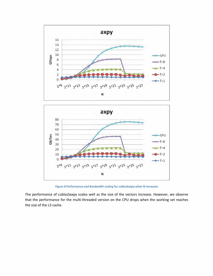
Figure 8 Performance and Bandwidth scaling for cublasSaxpy when N increases

The performance of cublasSaxpy scales well as the size of the vectors increase. However, we observe

that the performance for the multi-threaded version on the CPU drops when the working set reaches

the size of the L3 cache.

Figure 9 Performance and Bandwidth scaling for vecvec (psolve with simple Jacobi preconditioner) when N increases

Similarly to axpy we observe smooth scaling for the GPU while the performance for the multi-threaded

version on the CPU drops when the size of L3 is reached.. Note that we do not present results for the

blocked Jacobi preconditioner because in CUDA this involves calling cublasStrsm() two times for every

diagonal sub-block of matrix A. Since these blocks are small, typically of size 50, there are many of them.

Because the size of the blocks are small the GPU is underutilized in cublasStrsm(). Moreover, there is a

lot of overhead for calling cublasStrsm() many times.

Figure 10 Performance and Bandwidth scaling for our implementation of matvec when N increases and NZ/N remains con-stant

Similarly to the previous functions we observe smooth scaling for the GPU while the performance for

the multi-threaded version on the CPU drops when the size of L3 is reached.

Figure 11 Performance and Bandwidth scaling of matvec when the ratio NZ/N increases

When the number of non-zero elements per row (NZ/N) increases (0<NZ<N2 and 0 <NZ/N<N but NZ/N

has to be small so that A is sparse) we see that the performance of the CPU is kept almost constant and

always lower than the GPU performance of both our implementations with one thread/row and one

warp/row. This happens because at the dimension N=223 the performance of the threads is bandwidth

limited (the problem does not fit in the L3 cache anymore) therefore further increasing the number of

elements does not improve performance. However this is not the case for the GPU. The thread per row

implementation achieves very good performance when the array has very few non-zero elements, spe-

cifically when A is diagonal (NZ/N = 1) it reaches more than 5.5 Gflops and then as the number of non-

zero elements increases performance drops. Quite the opposite case appears for the warp/row imple-

mentation. Gflops are small for small NZ/N ratio and grow linearly until the ratio NZ/N is approximately

15. Then performance flattens. The behavior of the two implementation is due to the memory coalesc-

ing. As NZ/N increases the number of elements per row increases (our matrix generator guarantees that

the non-zero elements are evenly distributed to different rows). Therefore when the number of ele-

ments is small memory coalescing takes place for the thread/row implementation because memory ac-

cesses of threads operating on different row are being coalesced together. However, when the element

per row is big enough (>15) the coalescing cannot not take place anymore (values from different rows

are not close enough). It is exactly the opposite case for the warp/row implementation. Originally there

are not many idle threads created since there are not enough elements per row to operate on. Howev-

er, when NZ/N is high enough, the threads of a warp access neighboring memory locations which are

being coalesced.

We should also comment on the ratio of peak bandwidth we achieve over the maximum achievable

bandwidth. The above bandwidth plots correspond to the number of bytes that need to be read or writ-

ten over the execution time. cublasSdot achieves 80/102 = 78%, cublasSaxpy achieves 48/102 = 47%

and our implementations of vecvec reaches 45/102 = 44% [3,4]. Apparently, cublas are more optimized

than our simple vecvec kernel. Finally, matvec reaches up to 37/102=36%.

Conclusions In this project we have successfully used all three technologies taught in class: OpenMP, MPI, Cuda. We

have demonstrated speedups for all three and explored the performance benefits when we run our CG

application within a node, when employing multiple nodes and when we run it on a single GPU. Our op-

timizations addressed communication costs and workload distribution for MPI and memory coalescing

and data reuse for GPU.

We presented results across datasets with different characteristics in terms of density, size and distribu-

tion of non-zero elements. How sparse/dense the matrix A is determines how much computation exists

in an already memory-bound application and therefore how much benefit can be acquired from addi-

tional parallelism. The latter verifies the common knowledge that the choice of technology and optimi-

zations heavily depends on the application specifics (the characteristics of A). GPU will perform better

for CG matrixes that are big with significant number of non-zero elements, however cannot compete

with multiple nodes running multiple threads with low communication cost. When the number of nodes

increases to the level that communication cost is high the performance for multiple nodes with multiple

threads drops again.

Our results also demonstrate the fundamental differences between the way modern CPU and GPU pro-

cessors deal with memory latency. The former heavily rely on caching to hide that latency while the lat-

ter on multi-threading. When the working set does not fit inside the cache performance will drop dra-

matically, while for the GPUs this will be the case when there is not sufficient work to keep the hard-

ware threads busy.

References [1] “An Introduction to the Conjugate Gradient Method Without the Agonizing Pain”, Jonathan Richard

Shewchuk , August 4, 1994.

[2] Intel tutorial on sparse matrix storage formats

http://www.intel.com/software/products/mkl/docs/webhelp/appendices/mkl_appA_SMSF.html

*3+ “Benchmarking GPUs to Tune Dense Linear Algebra”, Vasily Volkov and James W. Demmel, SC '08:

Proceedings of the 2008 ACM/IEEE conference on Supercomputing

[4] NVIDIA Tesla C1060 specifications

http://www.nvidia.com/object/product_tesla_c1060_us.html

Self Evaluation and Milestones 1)

A. Nikolaos Trogkanis

B. Vasileios Kontorinis

2)

A(days) B(days)

Meetings 1 1

Coding 14 4

Writeup / Presentation 3 5

planning (alone) 3 1

total 21 11

3) Nikolaos was the person who pulled through the vast bulk of the coding part. He has dedicated much

more time in it than Vasileios, due to the fact that he was already familiar with MPI and OpenMP tech-

nology together with being way more efficient in delivering high quality code in short time. Vasileios put

more time in the presentation and writeup while actively contributing to the measurement collection

and plotting.

4) In a way, our team tried to optimize resource allocation by having each member focus on what can do

best. At the end of the day, the project reached an end within the time frame which constitutes a suc-

cess. (Vasileios, indeed, owes a beer to Nikolaos… :-)