Lecture 10: Finish Chapter 6; Chapter 7, Section 1 Random

©2011 Brooks/Cole, Cengage Learning

Elementary Statistics: Looking at the Big Picture 1

Lecture 10: Finish Chapter 6; Chapter 7, Section 1Random VariablesoIndependenceoRandom Variables: Definitions, NotationoProbability DistributionsoApplication of Probability RulesoMean and s.d. of Random Variables; Rules


Elementary Statistics: Looking at the Big Picture L10.2

Looking Back: Review

o 4 Stages of Statisticsn Data Production (discussed in Lectures 1-3)n Displaying and Summarizing (Lectures 3-8)n Probability

o Finding Probabilitieso Random Variableso Sampling Distributions

n Statistical Inference



Testing for IndependenceThe concept of independence is tied in with

conditional probabilities. Looking Ahead: Much of statistics concerns itself

with whether or not two events, or two variables, are dependent (related).



Example: Intuiting Conditional Probabilities When Events Are Dependento Background: Students are classified according to gender,

M or F, and ears pierced or not, E or not E .

o Questions:n Should gender and ears pierced be dependent or independent?

If dependent, which should be less, P(E) or P(E given M)?n What are the above probabilities, and which is less?

o Responses:n ____________Expect P(E given M) __________ P(E) because fewer

__________have pierced ears. n P(E given M) =_______________ P(E) = ________________

Practice: 6.18a-c p.254



Example: Intuiting Conditional Probabilities When Events Are Independento Background: Students are classified according to gender,

M or F, and whether they get an A in stats.

o Questions:n Should gender and getting an A or not be dependent or independent?

How should P(A) and P(A given F) compare?n What are the above probabilities, and how do they compare?

o Responses:n _____________. Expect P(A given F)____P(A) because knowing a

student’s gender doesn’t impact probability of getting an A.n P(A)=_____; P(A given F)=___________________

Practice: 6.19a,b p.254



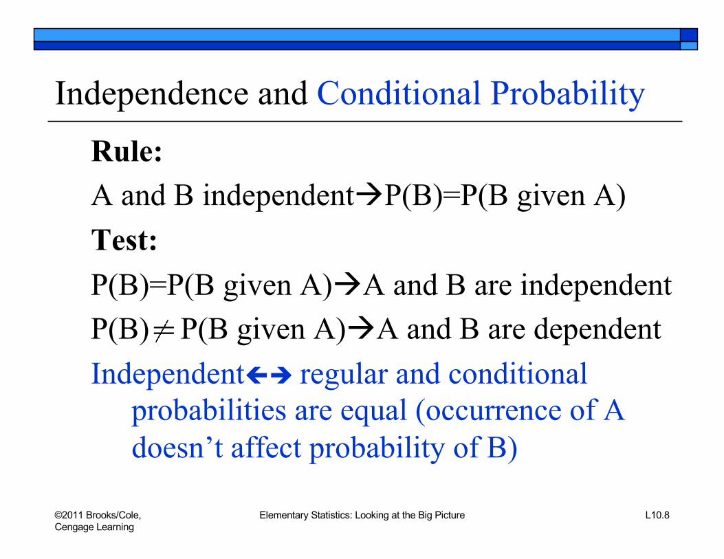
Independence and Conditional ProbabilityRule:A and B independentàP(B)=P(B given A)Test:P(B)=P(B given A)àA and B are independentP(B) P(B given A)àA and B are dependentIndependentçè regular and conditional

probabilities are equal (occurrence of A doesn’t affect probability of B)



Table of Counts Expected if Independentn For A, B independent,

P(A and B)=P(A)´P(B).n This Rule dictates what counts would

appear in two-way table if the variable A or not A is independent of the variable B or not B:

n If independent, count in category-combination A and B must equal total in A times total in B, divided byoverall total in table.



Example: Counts Expected if Independento Background: Students are classified according to gender

and ears pierced or not. A table of expected counts ( etc.) has been produced.

o Question: How different are the observed and expected counts?

o Response: Observed and expected counts are very different (270 vs. 174, 20 vs. 116, etc.) because

Practice: 6.18e-j p.254



Example: Counts Expected if Independento Background: Students are classified according to gender

and grade (A or not). A table of expected counts ( , etc.) has been produced.

o Question: How different are the observed and expected counts?

o Response: Counts are identical because

Obs A not A Total

F 15 45 60

M 10 30 40

Total 25 75 100

Exp A not A Total

F 15 45 60

M 10 30 40

Total 25 75 100

Practice: 6.19d-f p.255



Looking Back: Review

o 4 Stages of Statisticsn Data Production (discussed in Lectures 1-3)n Displaying and Summarizing (Lectures 3-8)n Probability

o Finding Probabilities (discussed in Lectures 9-10)o Random Variableso Sampling Distributions

n Statistical Inference



DefinitionRandom Variable: a quantitative variable whose

values are results of a random process

Looking Ahead: Sample proportion and sample mean are very complicated random variables. We start out by looking at much simpler random variables.

Looking Ahead: In Inference, we’ll want to draw conclusions about population proportion or mean, based on sample proportion or mean. To accomplish this, we will explore how sample proportion or mean behave in repeated samples. If the samples are random, sample proportion or sample mean are random variables.



Definitionsn Discrete Random Variable: one whose

possible values are finite or countably infinite (like the numbers 1, 2, 3, …)

n Continuous Random Variable: one whose values constitute an entire (infinite) range of possibilities over an interval



NotationRandom Variables are generally denoted with

capital letters such as X, Y, or Z.The letter Z is often reserved for random

variables that follow a standardized normal distribution.



Example: A Simple Random Variable

o Background: Toss a coin twice, and let the random variable X be the number of tails appearing.

o Questions: n What are the possible values of X?n What kind of random variable is X?

o Responses: n Possible values: n X is a _______________________

Practice: 7.1a p.285



Definitionsn Probability distribution of a random

variable tells all of its possible values along with their associated probabilities.

n Probability histogram displays possible values of a random variable along horizontal axis, probabilities along vertical axis.



Definitionn Probability distribution of a random

variable tells all of its possible values along with their associated probabilities.Looking Back: Last chapter we considered individual probabilities like the chance of getting two tails in two coin tosses. Now we take a more global perspective, considering the probabilities of all the possible numbers of tails occurring in two coin tosses.



Median and Mean of Probability Distribution

n Median is the middle value, with half of values above and half below (equal area value on histogram).

n Mean is average value (“balance point” of histogram)

n Mean equals Median for symmetric distributions



Example: Probability Distribution of a Random Variableo Background: The random variable X is the number of tails

in two tosses of a coin. o Questions:

n What are the probabilities of the possible outcomes?n What is the probability distribution of X?

o Responses: Possible outcomes:

Each has probability ____ so the probability distribution is:

Non-overlapping “Or” RuleàP(X=1) =________Practice: 7.1b p.285



Example: Probability Distribution of a Random Variable

o Background: We have the probability distribution of the random variable X for number of tails in two tosses of a coin.

o Question: How do we display and summarize X?

o Response: Use _____________________.Summarize: (center)(spread)

(shape)

mean=median=___

Typical distance from 1 is a bit less than ___.____________________

Practice: 7.3 p.286



Notation; Permissible Probabilities and Sum-to-One Rule for Probability Distributions

P(X=x) denotes the probability that the random variable Xtakes the value x.

Any probability distribution of a discrete random variable X must satisfy:

n where x is any value of Xn

where are all possible values of XAccording to this Rule, if a probability histogram has bars of

width 1, their total area must be 1.



Interim TableTo construct probability distribution for more

complicated random processes, begin with interim table showing all possible outcomes and their probabilities.



Example: Interim Table and Probability Distribution

o Background: A coin is tossed 3 times and the random variable X is number of tails tossed.

o Questions: What are the possible outcomes, values of X, and probabilities? How do we find probability that X =1? X =2?

o Response: n Interim Table:n Use ____________________

Rule to combine probabilities




Example: Probability Distribution and Histogram

o Background: X is number of tails in 3 coin tosses.o Question: What are the probability distribution of X and

probability histogram?o Response: Use the interim table to determine probabilities.

Use the probability distribution to sketch the histogram.

Practice: 7.5a-b p.286



Example: Summaries from Probability Histogram

o Background: Histogram for number of tails in 3 coin tosses.

o Question: What does it show?o Response:

Histogram has o Shape:o Center:o Spread:

median=mean=____Typical distance from mean a bit less than ____ since 1 and 2 (which are more common) are only 0.5 away from 1.5; 0 and 3 (less common) are 1.5 away from 1.5.

Looking Ahead: Standard deviation of R.V. to be introduced later on.

__________________

Practice: 7.5c p.286



Definition (Review)o Probability: chance of an event occurring,

determined as then Proportion of equally likely outcomes comprising

the event; orn Proportion of outcomes observed in the long run

that comprised the event; orn Likelihood of occurring, assessed subjectively.Looking Back: Principle of equally likely outcomes was

used to establish coin-flip probabilities. For other R.V.s, like household size, the distribution has been constructed for us based on long-run observations.



Example: Different Ways to Assess Probabilitieso Background: Census Bureau reported distribution of U.S.

household size in 2000.

o Question: What is the difference between how these probabilities have been assessed, and the way we assessed probabilities for coin-flip examples?

o Response: Coin-flip probabilities are based on ____________________________ (two equally likely faces).Household probabilities are based on _______________________ (all households in U.S. in 2000).

Practice: 7.7b p.287



Probability Rules (Review)Probabilities must obeyn Permissible Probabilities Rulen Sum-to-One Rulen “Not” Rulen Non-Overlapping “Or” Rulen Independent “And” Rulen General “Or” Rulen General “And” Rulen Rule of Conditional Probability



Example: Permissible Probabilities Rule

o Background: Household size in U.S. has

o Question: How do these probabilities conform to the Permissible Probabilities Rule?

o Response:



Example: Sum-to-One Rule


o Question: According to the “Sum-to-One” Rule, what must be true about the probabilities in the distribution?

o Response: According to the Rule, we have




Example: “Not” Rule


o Question: According to the “Not” Rule, what is the probability of a household notconsisting of just one person?

o Response:



Example: Non-Overlapping“Or” Rule


o Question: According to the Non-overlapping “Or” Rule, what is the probability of having fewer than 3 people?

o Response: The probability of having fewer than 3 people is P(X<3)= ________________________________________

Practice: 7.8a-b p.287



Example: Independent“And” Ruleo Background: Household size in U.S. has

o Question: Suppose a polling organization has sampled two households at random. According to the Independent “And” Rule, what is the probability that the first has 3 people and the second has 4 people?

o Response: The probability that the first has 3 people and the second has 4 people is

P(X1=3 and X2=4)=________________________________________where we use X1 to denote number in 1st household,

X2 to denote number in 2nd household.Practice: 7.8e p.287



Example: General“Or” Ruleo Background: Household size in U.S. has

o Question: Suppose a polling organization has sampled two households at random. According to the General “Or” Rule, what is the probability that one or the other has 3 people?

o Response: The events overlap: it is possible that both households have 3 people. P(X1=3 or X2=3) = __________________________________ _____________________________

where we apply the Independent “And” Rule for P(X1=3 and X2=3).

Practice: 7.8f p.287



Example: Rule of Conditional Probability


o Question: Suppose a polling organization samples only from households with fewer than 3 people. What is the probability that a household with fewer than 3 people has only 1 person?

o Response: P(X=1 given X<3) =

Practice: 7.8g p.287



Mean and Standard Deviation of Random Variable

o Mean of discrete random variable X

Mean is weighted average of values, where each value is weighted with its probability.

o Standard deviation of discrete random variable X

Standard deviation is “typical” distance of values from mean. Squared standard deviation is the variance.

Looking Back: Greek letters are used because these are the mean and standard deviation of all the random variables’ values.



Example: Mean of Random Variable


o Question: What is the mean household size?o Response: 1(0.26)+2(0.34)+…7(0.01) = ____ is the

mean household size.Looking Back: Median is 2 (has 0.5 at or below it). Mean is greater than median because distribution is skewed right. Also, mean is less than the “middle” number, 4, because smaller household sizes are weighted with higher probabilities.

Practice: 7.10g-h p.288



Example: Standard Deviation of R.V.o Background: Household size in U.S. has

o Question: What is the standard deviation of household sizes (typical distance from the mean, 2.5)? (a) 0.014 (b) 0.14 (c) 1.4 (d) 14.0

o Response: The typical distance of household sizes from their mean, 2.5, is ___: the closest are 0.5 away (2 and 3), the farthest is 4.5 away (7). (Or calculate by hand or with software).

Standard deviation =___

A Closer Look: Skewed rightà most of the spread arises from values above the mean, not below.

Practice: 7.15c p.288



Rules for Mean and Variance n Multiply R.V. by constantàits mean and

standard deviation are multiplied by same constant [or its abs. value, since s.d.>0]

n Take sum of two independent R.V.sào mean of sum = sum of meanso variance of sum = sum of variances (variance is squared standard deviation)

Looking Ahead: These rules will help us identify mean and standard deviation of sample proportion and sample mean.



Example: Mean, Variance, and SD of R.V.

o Background: Number X rolled on a die has

o Question: What are the mean, variance, and standard deviation of X?

o Response:n Mean: same as median ___ (because symmetric)n Variance: ____ (found by hand or with software)n Standard deviation:___(square root of variance)

Practice: 7.12 p.288



Example: Mean and SD for Multiple of R.V.o Background: Number X rolled on a die has mean 3.5, s.d.

1.7.

o Question:What are mean and s.d. of double the roll?o Response: For double the roll, mean is __________,

s.d. is _______________Practice: 7.15h-i p.289



Example: Mean and SD for Sum of R.V.so Background: Numbers X1, X2 on 2 dice each have mean

3.5, variance 2.92.

o Question:What are mean, variance, and s.d. of total on 2 dice?

o Response:Mean ___________, variance ________________, s.d. __________________

Practice: 7.84 p.340



Example: Doubling R.V. or Adding Two R.V.so Background: Double roll of a die: mean=7, s.d.= 3.4.

Total of 2 dice: mean=7, s.d.= 2.4.

o Question: Why is double roll more spread than total of 2 dice?o Response: Doubling roll of 1 die makes _______ [2(1)=2 or

2(6)=12] more likely; totaling 2 dice tends to have low and high rolls “cancel each other out”.

Practice: 7.84b p.340



Example: Doubling R.V. or Adding Two R.V.s

o This is the key to the benefits of sampling many individuals: The average of their responses gets us closer to what’s true for the larger group.

o If the numbers on a die were unknown, and you had to guess their mean value, would you make a better guess with a single roll or the average of two rolls?

?? ?



Lecture Summary(Finishing Probability Rules; Random Variables)

o Independence in context of Probabilityo Random variables

n Discrete vs. continuousn Notation

o Probability distributions: displaying, summarizingo Probability rules applied to random variableso Constructing distribution tableo Mean and standard deviation of random variableo Rules for mean and variance

Documents

Lecture 10: Finish Chapter 6; Chapter 7, Section 1 Random