Chapter 4 Continuous Random Variables - Purdue University · Chapter 4 Continuous Random Variables A random variable can be discrete, continuous, or a mix of both. Discrete random

Chapter 4

Continuous Random Variables

A random variable can be discrete, continuous, or a mix of both. Discrete random variablesare characterized through the probability mass functions, i.e., the ideal histograms. However,the same argument does not hold for continuous random variables because the width of eachhistogram’s bin is now infinitesimal. In this chapter we will generalize PMF to a new conceptcalled probability density function, and derive analogous properties.

4.1 Probability Density Function

To understand how a continuous random variable can be characterized, we start by general-izing the probability mass function.

Let X be a discrete random variable. In principle, we should consider the states of X as acountable sequence because X is discrete. However, for the time being let us consider X ascontinuous. Let x0 be one of its states, and suppose that there is an interval [a, b] such thatfor any x ∈ [a, b],

pX(x) =

0, if x 6= x0,

p0, if x = x0.

Then, according to the definition of PMF, the probability of a ≤ X ≤ b is defined as

P[a ≤ X ≤ b](a)= P[X = x0] = p0

(b)=

∫ b

a

p0 δ(x− x0)︸︷︷︸fX(x)

dx. (4.1)

In this equation, (a) holds because there is no other non-zero probabilities in the interval[a, b] besides x0. The integration in (b) follows from the definition of a delta function, whichis that δ(x− x0) =∞ if x = x0, δ(x− x0) = 0 if x 6= x0, and∫ ∞

−∞δ(x− x0)dx = 1.

1

That is, if we integrate the delta function then we will obtain one. If we further define

fX(x)def= p0 δ(x− x0), then the right hand side of Equation (4.1) provides a density charac-

terization of the random variable X: When we integrate the density function fX(x), we willobtain the probability. Figure 4.1 shows an illustration.

Figure 4.1: PMF is a train of impulses, whereas PDF is (usually) a smooth function.

Continuous random variables have a smooth density function as illustrated on the righthand side of Figure 4.1. The characterization, however, is the same as Equation (4.1). Thefollowing definition summarizes this.

Definition 1. The probability density function (PDF) of a random variable X is afunction which, when integrated over an interval [a, b], yields the probability of obtaininga ≤ X ≤ b. We denote PDF of X as fX(x), and

P[a ≤ X ≤ b] =

∫ b

a

fX(x)dx. (4.2)

Example 1. Let X be the phase angle of a voltage signal. Without any prior knowledgeabout X we may assume that X has an equal probability of any value between 0 to 2π. Findthe PDF of X and compute P[0 ≤ X ≤ π/2].

Solution. Since X has an equal probability for any value between 0 to 2π, the PDF of X is

fX(x) =1

2π, for 0 ≤ x ≤ 2π.

Therefore, the probability P[0 ≤ X ≤ π/2] can be computed as

P[0 ≤ X ≤ π

2

]=

∫ π/2

0

1

2πdx =

1

4.

Remark: Note that when specifying the PDF of a continuous random variable, the rangeis very important, e.g., 0 ≤ x ≤ 2π in this example.

c© 2018 Stanley Chan. All Rights Reserved. 2

Example 2. Let X be a discrete random variable with PMF

pX(k) =1

2k, k = 1, 2, . . . ,

What is fX(x),the continuous representation of pX(k)? Find the probability P[1 ≤ X ≤ 3].

Solution. The continuous representation of the PMF can be written in terms of a train ofdelta functions:

fX(x) =∞∑k=1

(1

2k

)δ(x− k).

To see why this is the correct PDF, we can check a few x’s:

fX(1) =∞∑k=1

(1

2k

)δ(1− k) =

1

2,

fX(2) =∞∑k=1

(1

2k

)δ(2− k) =

1

4,

where in both examples δ(1 − k) = 1 only when k = 1 and δ(2 − k) = 1 only when k = 2.The probability P[1 ≤ X ≤ 3] can be computed as

P[1 ≤ X ≤ 3] =

∫ 3

1

fX(x)dx =

∫ 3

1

∞∑k=1

(1

2k

)δ(x− k)dx

=∞∑k=1

(1

2k

)∫ 3

1

δ(x− k)dx =3∑

k=1

(1

2k

)=

7

8.

Normalization Property

Same as the discrete random variable, the continuous random variable should have its PDFintegrated to one.

Theorem 1. A PDF fX(x) should satisfy∫ ∞−∞

fX(x)dx = 1. (4.3)

Proof. The proof follows from the fact that∫ ∞−∞

fX(x)dx = P[−∞ ≤ X ≤ ∞],

which must be 1 as x is integrated over the entire real line.


Example 3. Let fX(x) = c(1− x2) for −1 ≤ x ≤ 1, and 0 otherwise. Find the constant c.

Solution. Since ∫ ∞−∞

fX(x)dx =

∫ 1

−1

c(1− x2)dx =4c

3,

and because∫∞−∞ fX(x)dx = 1, we have c = 3/4.

What is P[X = x0] if X is continuous?

The long answer will be discussed in the next section. The short answer is: If the PDF fX(x)(which is a function of x) is continuous at x = x0, then P[X = x0] = 0. This can be seenfrom the definition of the PDF. As a→ x0 and b→ x0, the integration interval becomes 0.Thus, unless fX(x) is a delta function at x0, which has been excluded because we assumedfX(x) is continuous at x0, the integration result must be zero.

4.2 Cumulative Distribution Function

Definition 2. The cumulative distribution function (CDF) of a continuous randomvariable X is

FX(x)def= P[X ≤ x] =

∫ x

−∞fX(x′)dx′. (4.4)

If we compare this definition with the one for discrete random variable, we see that the CDFfor a continuous random variable X simply replaces the summation of a discrete randomvariable by integration. Therefore, we should expect more of the properties to inherit fromthe discrete CDF.

Example. Let X be a continuous random variable with PDF

fX(x) =1

b− a, a ≤ x ≤ b.

Find the CDF of X.

Solution. The CDF of X is given by

FX(x) =

∫ x

−∞fX(x′)dx′ =

∫ x

a

1

b− adx′ =

x− ab− a

,

for a ≤ x ≤ b. For x < a, FX(x) = 0, and for x > b, FX(x) = 1.


Properties of CDF

We now describe the properties of a CDF.

Proposition 1. Let X be a random variable (either continuous or discrete), then the CDFof X has the following properties:

(i) The CDF is a non-decreasing.

(ii) The maximum of the CDF is when x =∞: FX(+∞) = 1.

(iii) The minimum of the CDF is when x = −∞: FX(−∞) = 0.

Pictorially, these properties are illustrated from Figure 4.2: (i) follows from the fact that weare integrating a non-negative function fX(x). Thus the bigger the x the more areas we willintegrate under the curve. (ii) and (iii) indicate the two extreme values of the CDF.

Figure 4.2: A CDF is the integration of the PDF. Thus, the height of a stem in the CDFcorresponds to the area under the curve of the PDF.

The next property relates probability and CDF.

Proposition 2. Let X be a continuous random variable. If the CDF FX is continuous atany a ≤ x ≤ b, then

P[a ≤ X ≤ b] = FX(b)− FX(a). (4.5)

Proof. The proof follows from the definition of the CDF, which states that

FX(b)− FX(a) =

∫ b

−∞fX(x′)dx′ −

∫ a

−∞fX(x′)dx′ =

∫ b

a

fX(x′)dx′ = P[a ≤ X ≤ b].

This result shows that for a continuous random variable X, P[X = x0] = FX(x0)−FX(x0) =0. (That is, substitute a = x0 and b = x0 in the above equation.) Intuitively, this can beexplained from the fact that the integration interval is infinitesimally small.


The next two propositions concern about the discontinuity of the CDF.

Definition 3. The CDF FX(x) is said to be

• Left-continuous at x = b if FX(b) = FX(b−)def= limh→0 FX(b− h);

• Right-continuous at x = b if FX(b) = FX(b+)def= limh→0 FX(b+ h);

• Continuous at x = b if it is both right-continuous and left-continuous at x = b. Inthis case, we have

limh→0

FX(b− h) = limh→0

FX(b+ h) = F (b).

In this definition, the step size h > 0 is shrinking to zero. The point b− h stays at the leftof b, and b + h stays at the right of b. The limits on the left hand side and the right handside are not necessarily equal, unless the function Fx(x) is continuous at x = b.

Proposition 3. For any random variable X (discrete or continuous), FX(x) is right-continuous. That is,

FX(b) = FX(b+)def= lim

h→0FX(b+ h) (4.6)

Right-continuous essentially means that if FX(x) is piecewise, then it must have a solid leftend and an empty right end. If FX(x) is continuous at x = b, then the leftmost soliddot will overlap with the rightmost empty dot of the previous segment. Thus, there is nogap between the two. A pictorial illustration is shown in Figure 4.3.

Figure 4.3: Illustration of right continuous.

Proposition 4. For any random variable X (discrete or continuous), P[X = b] is

P[X = b] =

FX(b)− FX(b−), if FX is discontinuous at x = b

0, otherwise.(4.7)

This proposition concerns about the probability at discontinuity. It states that when FX(x)is discontinuous at x = b, then P[X = b] is the difference between FX(b) and the limit fromthe left. In other words, the height of the gap determines the probability at discontinuity.If FX(x) is continuous at x = b, then FX(b) = limh→0 FX(b− h) and so P[X = b] = 0.


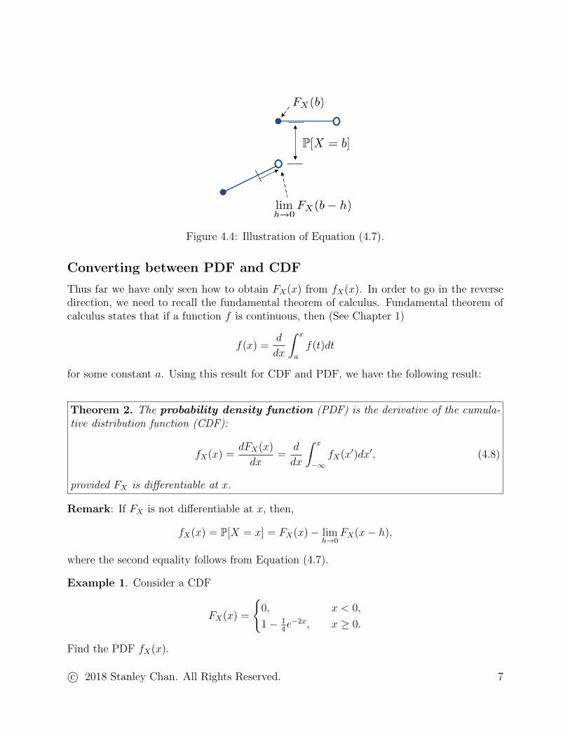
Figure 4.4: Illustration of Equation (4.7).

Converting between PDF and CDF

Thus far we have only seen how to obtain FX(x) from fX(x). In order to go in the reversedirection, we need to recall the fundamental theorem of calculus. Fundamental theorem ofcalculus states that if a function f is continuous, then (See Chapter 1)

f(x) =d

dx

∫ x

a

f(t)dt

for some constant a. Using this result for CDF and PDF, we have the following result:

Theorem 2. The probability density function (PDF) is the derivative of the cumula-tive distribution function (CDF):

fX(x) =dFX(x)

dx=

d

dx

∫ x

−∞fX(x′)dx′, (4.8)

provided FX is differentiable at x.

Remark: If FX is not differentiable at x, then,

fX(x) = P[X = x] = FX(x)− limh→0

FX(x− h),

where the second equality follows from Equation (4.7).

Example 1. Consider a CDF

FX(x) =

0, x < 0,

1− 14e−2x, x ≥ 0.

Find the PDF fX(x).


Figure 4.5: Example 1.

Solution. First, it is easy to show that FX(0) = 34. This corresponds to a discontinuity at

x = 0, as shown in Figure 4.5. Because of the discontinuity, we need to consider three whendetermining fX(x):

fX(x) =

dFX(x)dx

, x < 0,

P[X = 0], x = 0,dFX(x)dx

, x > 0.

When x < 0, FX(x) = 0. So, dFX(x)dx

= 0.

When x > 0, FX(x) = 1− 14e−2x. So, dFX(x)

dx= 1

2e−2x.

When x = 0, the probability P[X = 0] is determined according to Property 7 which is theheight between the solid dot and the empty dot. This yields

P[X = 0] = FX(0)− limh→0

FX(0− h) =3

4− 0 =

3

4.

Therefore, the overall PDF is

fX(x) =

0, x < 0,34, x = 0,

12e−2x, x > 0.

4.3 Expectation, Variance and Moments

Definition 4. The expectation of a continuous random variable X is

E[X] =

∫ ∞−∞

x fX(x)dx. (4.9)

If g is a function, then

E[g(X)] =

∫ ∞−∞

g(x) fX(x)dx. (4.10)


Example 1. Let Θ be a continuous random variable with PDF fΘ(θ) = 12π

. Let Y =cos(ωt+ Θ). Find E[Y ].

Solution. Referring to Equation (4.10), the function g is g(θ) = cos(ωt+ θ). Therefore, theexpectation E[Y ] is

E[Y ] =

∫ 2π

0

cos(ωt+ θ)fΘ(θ)dθ =1

2π

∫ 2π

0

cos(ωt+ θ)dθ = 0,

where the last equality holds because integrating a sinusoid over one period is 0.

Example 2. Let IΩ(X) be an indicator function such that

IΩ(X) =

1, if X ∈ Ω,

0, if X 6∈ Ω.

Find E[IΩ(X)].

Solution. The expectation is

E[IΩ(X)] =

∫ ∞−∞

IΩ(x)fX(x)dx =

∫x∈Ω

fX(x)dx = P[X ∈ Ω].

This result shows that the probability of an event X ∈ Ω can be equivalently representedin terms of expectation.

Existence of Expectation

Not all random variables has expectation. Only random variables that are absolutely inte-grable can have expectation.

Definition 5. A random variable X is said to be absolutely integrable if

E[|X|] =

∫ ∞−∞|x|fX(x)dx <∞. (4.11)

Before we discuss an example, we should clarify that the limits of the integration in Equa-tion (4.9) should be sent to infinity separately. That is,

E[X] =

∫ ∞−∞

x fX(x)dx = lima→−∞

limb→∞

∫ b

a

x fX(x)dx.

Note that

lima→−∞

limb→∞

∫ b

a

x fX(x)dx 6= limT→∞

∫ T

−Tx fX(x)dx.


The interpretation of the double limit is that we can decompose∫ ∞−∞

x fX(x)dx = lima→−∞

∫ 0

a

x fX(x)dx+ limb→∞

∫ b

0

x fX(x)dx,

and each integral has to be finite in order to ensure the expectation exists.

Example 3. Let X be a Cauchy random variable with PDF

fX(x) =1

π(1 + x2). (4.12)

Show that the expectation of X does not exist.

Solution. From the definition of expectation, we know that

E[X] =

∫ ∞−∞

x · 1

π(1 + x2)dx =

1

π

∫ ∞0

x

(1 + x2)dx+

1

π

∫ 0

−∞

x

(1 + x2)dx.

The first integral gives ∫ ∞0

x

(1 + x2)dx =

1

2log(1 + x2)

∣∣∣∞0

=∞,

and the second integral gives −∞. Since neither integral is finite, the expectation is unde-fined. We can also check the absolutely integrable criteria:

E[|X|] =

∫ ∞0

|x| · 1

π(1 + x2)dx

(a)= 2

∫ ∞0

x

π(1 + x2)dx ≥ 2

∫ ∞1

x

π(1 + x2)dx

(b)

≥ 2

∫ ∞1

x

π(x2 + x2)dx =

1

πlog(x)

∣∣∣∞1

=∞,

where in (a) we use the fact that the function being integrated is even, and in (b) we lowerbound 1

1+x2≥ 1

x2+x2if x > 1.

Variance

Definition 6. The variance of a continuous random variables X is

Var[X] = E[(X − µX)2] =

∫ ∞−∞

(x− µX)2fX(x)dx, (4.13)

where µXdef= E[X].

It is not difficult to show that the variance can also be expressed as

Var[X] = E[X2]− µ2X ,

because

Var[X] = E[(X − µX)2] = E[X2]− 2E[X]µX + µ2X = E[X2]− µ2

X .


4.4 Mean, Mode, Median

There are three statistical quantities we are usually interested in: Mean, mode and median.It is possible to obtain these three quantities from PDF and CDF.

Mean

The mean of a random variable is also the expectation of the random variable. Therefore,the mean can be computed via the PDF as follows.

Definition 7. Let X be a random variable. The mean of X is

Mean = E[X] =

∫ ∞−∞

xfX(x)dx. (4.14)

Mean can also be computed from the CDF, shown in the following theorem.

Theorem 3. The mean of a random variable X can be computed from the CDF as

Mean = E[X] =

∫ ∞0

(1− FX(x′)) dx′ −∫ 0

−∞FX(x′)dx′. (4.15)

Proof. For any random variable X, we can partition X = X+ − X− where X+ and X−

are the positive and negative parts, respectively. Consider the positive part first. For anyX > 0, it holds that∫ ∞

0

(1− FX(x′)) dx′ =

∫ ∞0

[1− P[X ≤ x′]] dx′ =

∫ ∞0

P[X > x′]dx′

=

∫ ∞0

∫ ∞x′

fX(x)dxdx′ =

∫ ∞0

∫ x

0

fX(x)dx′dx

=

∫ ∞0

xfX(x)dx = E[X].

Now, consider the negative part. For any X < 0, it holds that∫ 0

−∞FX(x′)dx′ =

∫ 0

−∞P[X ≤ x′]dx′ =

∫ 0

−∞

∫ x′

−∞fX(x)dxdx′

=

∫ 0

−∞

∫ 0

x

fX(x)dx′dx =

∫ 0

−∞xfX(x)dx = E[X],

where in both cases we switched the order of the integration.


Median

Definition 8. The median of a random variable X is the point −∞ < c <∞ such that∫ c

−∞fX(x)dx =

∫ ∞c

fX(x)dx. (4.16)

Essentially, this means that the areas under the PDF on both sides of x = c are equal.

The median can also be evaluated from the CDF as follows.

Theorem 4. The median of a random variable X is the point c such that

FX(c) =1

2. (4.17)

Proof. Since FX(x) =∫ x−∞ fX(x′)dx′, we have

FX(c) =

∫ c

−∞fX(x)dx =

∫ ∞c

fX(x)dx = 1− FX(c).

Rearranging the terms shows that FX(c) = 12.

Mode

Definition 9. The mode of a random variable X is the point c such that fX(x) attains themaximum:

c = argmaxx

fX(x). (4.18)

The mode of a random variable is not unique, e.g., a mixture of two identical Gaussians withdifferent means has two modes.

Theorem 5. The mode of a random variable X is the point c such that the slope of FX(x)is maximized.

c = argmaxx

F ′X(x). (4.19)

Proof. Note that from the definition of CDF, we have

fX(x) =d

dx

∫ x

−∞fX(x′)dx′ =

d

dxFX(x) = F ′X(x).

Therefore,c = argmax

xfX(x) = argmax

xF ′X(x).

A pictorial illustration of mode and median is given in Figure 4.6.


Figure 4.6: Mode and median in a PDF and a CDF.

4.5 Common Continuous Random Variables

Uniform Random Variable

Definition 10. Let X be a continuous uniform random variable. The PDF of X is

fX(x) =

1b−a , a ≤ x ≤ b,

0, otherwise,(4.20)

where [a, b] is the interval on which X is defined. We write

X ∼ Uniform(a, b)

to say that X is drawn from a uniform distribution on an interval [a, b].

Uniform distribution can also be defined for discrete random variables. In this case, theprobability mass function is given by

pX(k) =1

b− a+ 1, k = a, a+ 1, . . . , b.

The presence of “1” in the denominator of the PMF is due to the fact that k runs from a tob, including the two end points.

The mean and variance of a uniform random variable is stated in the theorem below.

Theorem 6. If X ∼ Uniform(a, b), then

E[X] =a+ b

2, and Var[X] =

(b− a)2

12.


Proof. The proof follows from the definition of expectation and variance:

E[X] =

∫ ∞−∞

xfX(x)dx =

∫ b

a

x

b− adx =

a+ b

2

E[X2] =

∫ ∞−∞

x2fX(x)dx =

∫ b

a

x2

b− adx =

a2 + ab+ b2

3

Var[X] = E[X2]− E[X]2 =(b− a)2

12.

Example. (Quantization Error). Uniform distribution can be used to model quantizationerror in random signals. Let X[n] be a discrete time signal at time n. (X[n] has to berandom, and independent at every time instant.) The quantized signal using a quantizationstep ∆ is defined as

Xq[n] = ∆

[X[n]

∆

],

where [·] denotes the rounding operator. The quantization error is the difference betweenthe quantized sample and the true sample:

Eq[n] = X[n]−Xq[n].

The distribution of Eq[n] is approximately uniform, with Eq[n] ∼ Uniform[−∆

2, ∆

2

]. Then,

one can show that the quantization error power is

Pedef= Var[Eq[n]] =

∆2

12. (4.21)

Figure 4.7: Illustration of quantization, and the histogram of the error.


Exponential Random Variable

Definition 11. Let X be an exponential random variable. The PDF of X is

fX(x) =

λe−λx, x ≥ 0,

0, otherwise,(4.22)

where λ > 0 is a parameter. We write

X ∼ Exponential(λ)

to say that X is drawn from an exponential distribution of parameter λ.

The parameter λ of the exponential random variable determines the rate of decay. Thus, alarge λ implies a faster decay.

Figure 4.8: Exponential distribution

Theorem 7. If X ∼ Exponential(λ), then

E[X] =1

λ, and Var[X] =

1

λ2.

Proof.

E[X] =

∫ ∞−∞

xfX(x)dx =

∫ ∞0

λxe−λxdx = −∫ ∞

0

xde−λx

= −xe−λx∣∣∣∞0

+

∫ ∞0

e−λxdx =1

λ

E[X2] =

∫ ∞−∞

x2fX(x)dx =

∫ ∞0

λx2e−λxdx = −∫ ∞

0

x2de−λx

= −x2e−λx∣∣∣∞0

+

∫ ∞0

2xe−λxdx = 0 +2

λE[X] =

2

λ2

Var[X] = E[X2]− E[X]2 =1

λ2,

where we used integration by parts in calculating E[X] and E[X2].


Example. (Relation to Poisson). An exponential random variable can be derived from aPoisson random variable, which is of important interest in studying traffics. Let N be thenumber of people arriving at a station. We assume that N is Poisson with rate λ. Let Tbe the inter-arrival time between two people. Then, for any duration t, the probability ofobserving n people is

P[N = n] =(λt)n

n!e−λt.

Therefore,

P[T > t] = P[inter-arrival time > t] = P[no arrival in t] = P[N = 0] = e−λt.

Since P[T > t] = 1− FT (t), where FT (t) is the CDF of T , we can show that

fT (t) =d

dtFT (t) = λe−λt. (4.23)

That is, if N is Poisson with rate λ, then T is exponential with rate λ.

Gaussian Random Variable

Definition 12. Let X be an Gaussian random variable. The PDF of X is

fX(x) =1√

2πσ2e−

(x−µ)2

2σ2 (4.24)

where (µ, σ2) are parameters of the distribution. We write

X ∼ N (µ, σ2)

to say that X is drawn from a Gaussian distribution of parameter (µ, σ2).

Gaussian random variables are also called normal random variables. The parameters (µ, σ2)are the mean and the variance, respectively. Note that a Gaussian random variable has asupport from −∞ to ∞. Thus, fX(x) has a non-zero value for any x, even though the valueis extremely small. A Gaussian random variable is also symmetric about µ. If µ = 0, thenfX(x) is an even function.

Theorem 8. If X ∼ N (µ, σ2), then

E[X] = µ, and Var[X] = σ2. (4.25)


Proof. The expectation can be proved via substitution.

E[X] =1√

2πσ2

∫ ∞−∞

xe−(x−µ)2

2σ2 dx(a)=

1√2πσ2

∫ ∞−∞

(y + µ)e−y2

2σ2 dy

=1√

2πσ2

∫ ∞−∞

ye−y2

2σ2 dy +1√

2πσ2

∫ ∞−∞

µe−y2

2σ2 dy

(b)= 0 + µ

(1√

2πσ2

∫ ∞−∞

e−y2

2σ2 dy

)(c)= µ,

where in (a) we substitute y = x−µ, in (b) we use the fact that the first integrand is odd sothat the integration is 0, and in (c) we observe that integration over the entire sample spaceof the PDF yields 1.

The variance is also proved by substitution.

Var[X] =1√

2πσ2

∫ ∞−∞

(x− µ)2e−(x−µ)2

2σ2 dx

(a)=

σ2

√2π

∫ ∞−∞

y2e−y2

2 dy, by letting y =x− µσ

=σ2

√2π

(−ye−

y2

2

∣∣∣∞−∞

)+

σ2

√2π

∫ ∞−∞

e−y2

2 dy = 0 + σ2

(1√2π

∫ ∞−∞

e−y2

2 dy

)= σ2,

where in (a) we substitute y = (x− µ)/σ.

Standard Gaussian

In many practical situations, we need to evaluate the probability P[a ≤ X ≤ b] of a Gaussianrandom variable X. This involves integration of the Gaussian PDF, i.e. determining theCDF. Unfortunately, there is no closed-form expression of P[a ≤ X ≤ b] in terms of (µ, σ2).This leads to what we call the standard Gaussian.

Definition 13. A standard Gaussian (or standard Normal) random variable X has aPDF

fX(x) =1√2πe−

x2

2 . (4.26)

That is, X ∼ N (0, 1) is a Gaussian with µ = 0 and σ2 = 1.

Definition 14. The CDF of the standard Gaussian is defined as the Φ(·) function

Φ(y) =1√2π

∫ y

−∞e−

x2

2 dx (4.27)


Figure 4.9: Definition of Φ(y).

Theorem 9 (CDF of an arbitrary Gaussian). Let X ∼ N (µ, σ2). Then,

P[X ≤ b] = Φ

(b− µσ

). (4.28)

Proof. We start by expressing P[X ≤ b]:

P[X ≤ b] =

∫ b

−∞

1√2πσ2

e−(x−µ)2

2σ2 dx.

Substituting y = x−µσ

, and using the definition of standard Gaussian, we have∫ b

−∞

1√2πσ2

e−(x−µ)2

2σ2 dx =

∫ b−µσ

−∞

1√2πe−

y2

2 dy = Φ

(b− µσ

).

Corollary 1. Let X ∼ N (µ, σ2). Then,

P[a < X ≤ b] = Φ

(b− µσ

)− Φ

(a− µσ

). (4.29)

Proof. Applying the Gaussian CDF twice yields the desired result:

P[a < X ≤ b] = P[X ≤ b]− P[X ≤ a] = Φ

(b− µσ

)− Φ

(a− µσ

).

Note that in the above corollary, the inequality signs of the two end points are not important.That is, the statement also holds for P[a ≤ X ≤ b] or P[a < X < b], becauseX is a continuousrandom variable at every x. Thus, P[X = a] = P[X = b] = 0 for any a and b.


Properties of Φ(y)

Corollary 2. Let X ∼ N (µ, σ2). Then, the following results hold:

• Φ(y) = 1− Φ(−y).

• P[X ≥ b] = 1− Φ(b−µσ

).

• P[|X| ≥ b] = 1− Φ(b−µσ

)+ Φ

(−b−µσ

)Proof. Exercise.

4.6 Function of Random Variables

One common question we encounter in practice is the transformation of random variables.The question is simple: Given a random variable X with PDF fX(x) and CDF FX(x), andsuppose that Y = g(X) for some function g, then what are fY (y) and FY (y)?

General PrincipleIn general, this question can be answer by first looking at the CDF of Y :

FY (y) = P[Y ≤ y] = P[g(X) ≤ y]. (4.30)

If g is an invertible function, i.e., g−1 exists and gives an unique value, then

P[g(X) ≤ y] = P[X ≤ g−1(y)] = FX(g−1(y)). (4.31)

The CDF is the integration of the variable x

FX(g−1(y)) =

∫ g−1(y)

−∞fX(x′)dx′, (4.32)

and hence by fundamental theorem of calculus, we have

fY (y) =d

dyFY (y) =

d

dyFX(g−1(y))

=d

dy

∫ g−1(y)

−∞fX(x′)dx′

=

(d g−1(y)

dy

)· fX(g−1(y)). (4.33)

When g−1 does not attain a unique value, e.g., g(x) = x2 implies g−1(y) = ±√y. When thishappens, then instead of writing X ≤ g−1(y) we need to determine all possible X such thatg(X) ≤ y. The following examples will illustrate how we can do so.


Procedure.To make the above discussion short we summarize them into two major steps:

• Step 1: Find the CDF FY (y), which is P[Y ≤ y], using FX(x).

• Step 2: Find the PDF fY (y) by taking derivative on FY (y).

Let us now consider a few examples.

Example 1. Let X be a random variable with PDF fX(x) and CDF FX(x). Let Y = 2X+3.Find fY (y) and FY (y). Express answers in terms of fX(x) and FX(x).

Solution. We first note that

FY (y) = P[Y ≤ y] = P[2X + 3 ≤ y] = P[X ≤ y − 3

2

]= FX

(y − 3

2

).

Therefore, the PDF is

fY (y) =d

dyFY (y) =

d

dyFX

(y − 3

2

)= F ′X

(y − 3

2

)d

dy

(y − 3

2

)=

1

2fX

(y − 3

2

).

Example 2. Let X be a random variable with PDF fX(x) and CDF FX(x). Suppose thatY = X2, find fY (y) and FY (y). Express answers in terms of fX(x) and FX(x).

Solution. To solve this problem, we note that

FY (y) = P[Y ≤ y] = P[X2 ≤ y]

= P[−√y ≤ X ≤ √y]

= FX(√y)− FX(−√y).

Therefore, the PDF is

fY (y) =d

dyFY (y) =

d

dy(FX(

√y)− FX(−√y))

= F ′X(√y)d

dy

√y − F ′X(−√y)

d

dy(−√y)

=1

2√y

(fX(√y) + fX(−√y)) .


Example 3. Let X ∼ Uniform(0, 2π). Suppose Y = cosX. Find fY (y) and FY (y).

Solution. First of all, we need to find the CDF of X. This can be done by noting that

FX(x) =

∫ x

−∞fX(x′)dx′ =

∫ x

0

1

2πdx′ =

x

2π.

Thus, the CDF of Y is

FY (y) = P[Y ≤ y] = P[cosX ≤ y]

= P[cos−1 y ≤ X ≤ 2π − cos−1 y]

= FX(2π − cos−1 y)− FX(cos−1 y)

= 1− cos−1 y

π.

The PDF of Y is

fY (y) =d

dyFY (y) =

d

dy

(1− cos−1 y

π

)=

1

π√

1− y2,

where we used the fact that ddy

cos−1 y = −1√1−y2

.

Example 4. Let X be a random variable with PDF

fX(x) = aexe−aex

.

Let Y = eX , and find fY (y).

Solution. To solve this problem, we first note that

FY (y) = P[Y ≤ y] = P[eX ≤ y]

= P[X ≤ log y]

=

∫ log y

−∞aexe−ae

x

dx.

To find the PDF, we recall the fundamental theorem of calculus. This will give us

fY (y) =d

dy

∫ log y

−∞aexe−ae

x

dx

=

(d

dylog y

)(d

d log y

∫ log y

−∞aexe−ae

x

dx

)=

1

yaelog ye−ae

log y

= ae−ay.


4.7 Generating Random Numbers

For common types of random variables, e.g., Gaussian or exponential, there are often built-in functions to generate the random numbers. However, for arbitrary PDFs, how can wegenerate the random numbers?

Generating arbitrary random numbers can be done with the help of the following theorem.

Theorem 10. Let X be a random variable with an invertible CDF FX(x), i.e., F−1X exists.

If Y = FX(X), then Y ∼ Uniform(0, 1).

Proof. First, we know that if U ∼ Uniform(0, 1), then fU(u) = 1 for 0 ≤ u ≤ 1 and so

FU(u) =

∫ u

−∞fU(u)du = u,

for 0 ≤ u ≤ 1. If Y = FX(X), then the CDF of Y is

FY (y) = P[Y ≤ y] = P[FX(X) ≤ y]

= P[X ≤ F−1X (y)]

= FX(F−1X (y)) = y.

Therefore, we showed that the CDF of Y is the CDF of a uniform distribution. Thiscompletes the proof.

The consequence of the theorem is the following procedure in generating random numbers:

• Step 1: Generate a random number U ∼ Uniform(0, 1).

• Step 2: Let Y = F−1X (U). Then the distribution of Y is FX .

Example. Suppose we want to draw random numbers from an exponential distribution.Then, we can follow the above two steps as

• Step 1: Generate a random number U ∼ Uniform(0, 1).

• Step 2: Find F−1X . Since X is exponential, we know that FX(x) = 1 − e−λx. This

gives the inverse F−1X (x) = − 1

λlog(1 − x). Therefore, by letting Y = F−1

X (U), thedistribution of Y will be exponential.


Documents

Chapter 4 Continuous Random Variables - Purdue University · Chapter 4 Continuous Random Variables A random variable can be discrete, continuous, or a mix of both. Discrete random