Embed Size (px)
Citation preview

Lecture 1Introduction to Micorarrays and Concepts of Molecular Biology
M. Saleet Jafri
Program in Bioinformatics and Computational Biology
George Mason University

Lecture 1
Overview of Molecular and Cellular Biology
Biological References
• Molecular Biology of the Cellby Bruce Alberts(1994 or newer edition)
• Molecular Cell Biologyby Darnell, Lodish, and Baltimore (1995 or newer edition)

Part I: Molecular Biology Review
Where do biological sequences come from?
• Life and evolution• Proteins• Nucleic Acids• Central dogma• Genetic code• DNA structure• Mitochondrial DNA

Life• Evolved from common origin• ˜3.5 billion years ago• All life shares similar biochemistry
– Proteins: active elements– Nucleic acids: informational elements
• Molecular Biology: the study of structure and function of proteins and nucleic acids

Terrestrial Life

Cell typesProkaryotes – no nuclear membrane, represented by
cyanobacteria (blue-green algae) and common bacteria (Escherichia coli)
Eukaryotes – unicellular organisms such as yeast and multicellular organisms
Archaebacteria – no nuclear membrane but similar to eukaryotes in transcription and translation mechanisms, discovered in deep sea thermal vents in 1982

Prokaryotic Cell

Prokaryotic Cell
Eukaryotes• In eukaryotes, transcription is complex:
– Many genes contain alternating exons and introns– Introns are spliced out of mRNA– mRNA then leaves the nucleus to be translated by ribosomes
• Genomic DNA: entire gene including exons and introns– The same genomic DNA can produce different proteins by
alternative splicing of exons• Complementary DNA (cDNA): spliced sequence containing only
exons– cDNA can be manufactured by capturing mRNA and performing
reverse transcription

Eukaryotic Cell

Eukaryotic Cell

Eukaryotic Cell Organelles• Cell membrane• Nucleus• Cytoplasm• Endoplasmic Reticulum – rough and smooth• Golgi Apparatus – received newly formed proteins from the ER and
modifies them and directs them to final destination• Mitochondria – respiratory centers, have own circular DNA, bacterial
origin
Eukaryotic Cell Organelles
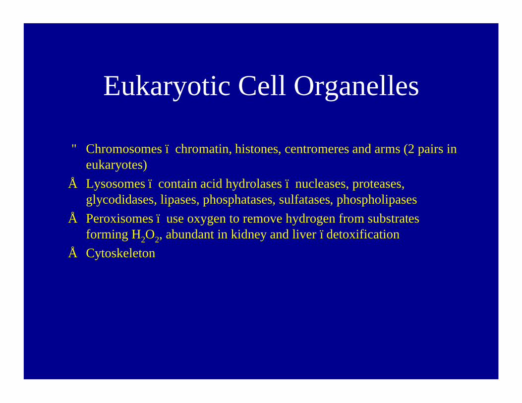
• Chromosomes – chromatin, histones, centromeres and arms (2 pairs in eukaryotes)
• Lysosomes – contain acid hydrolases – nucleases, proteases, glycodidases, lipases, phosphatases, sulfatases, phospholipases
• Peroxisomes – use oxygen to remove hydrogen from substrates forming H2O2, abundant in kidney and liver –detoxification
• Cytoskeleton

Eukaryotic Membrane

Nucleic Acids• Two kinds:
– RNA: ribonucleic acid– DNA: deoxyribonucleic acid

Nucleic Acid Structure

DNA• Double stranded• Four bases: adenine (A),
guanine (G), cytosine (C) andthymine (T)
• A and G are purines• C and T are pyrimidines• A always paired with T
(complementary)• C always paired with G
(complementary)=> Watson-Crick base pairs (bp)• DNA may consist of hundreds
of millions bp• A short sequence (<100) is
called an oligonucleotide

RNA• Different sugar (ribose instead of 2’-deoxyribose)• Uracil (U) instead of thymine (U binds with A)• RNA does not form a double helix• RNA may have a complex three-dimensional structure

Central Dogma
DNA → RNA → Protein
DNA = Deoxyribonucleic Acid
RNA = Ribonucleic Acid
Protein = Functional and Structural units of cells
Flow of Information is unidirectional


Gene Transcription or DNA Transcription
• RNA molecules synthesized by RNA polymerase• RNA polymerase found in free and bound form• RNA polymerase binds very tightly to promoter region on DNA• Promoter region contains start site• Transcription ends at termination signal site.• Primary transcript – direct coding of RNA from DNA• RNA splicing – introns removed to make the mRNA• mRNA – contains the sequence of codons that code for a protein• uracil replaces thymine• splicing and alternative splicing


Translation• Ribosomes made of protein and ribosomal RNA
(rRNA)• Transfer RNA (tRNA) make connection between
specific codons in mRNA and amino acids– As tRNA binds to the next codon in mRNA, its
amino acid is bound to the last amino acid in the protein chain
• When a STOP codon is encountered, the ribosome releases the mRNA and synthesis ends

Gene Translation• tRNA – links an amino acid to the codon on the mRNA via
the anit-codon• rRNA – RNA found in ribosomes• ribosomes – large and small subunit, made of protein and
rRNA• initiator tRNA always carries methionine• initiation factors – proteins that catayze the start of
transcription• stop codon• Endoplasmic Reticulum• Posttranscriptional modification

Translation• Involves ribosomes, and RNA• Ribosomes made of protein and RN A• Messenger RNA (mRNA) is the sequen ce transcribed
from the DN A• The mRNA is ‘threaded’ through the ribosomes.• Transfer RNA (tRNA) brings the different amino a cids to
the ribosome compl ex so that the amino acids can be attached to the grow ing amino acid chain.
Ribosome
Protein – amino acid chain
tRNA
Amino acidmRNA

Ribosome

Ribosomal RNA

Eukaryotic and Prokaryotic Ribosome Structure LSU
LSU
SSU
SSU


DNA Structure
• DNA contains:– Promoters– Genes– Junk DNA
• Reading frames• An open reading frames (ORF): a contiguous sequence of
DNA starting at a start codon and ending at a STOP codon


Chromosomes• A genome: a complete set of chromosomes within a cell• Different species have different numbers of chromosomes in their
genomes• Prokaryotes usually have a single chromosome, often a circular DNA
molecule• Eukaryotic chromosomes appear in pairs (diploid), each inherited from
one parent– Homologous chromosomes carry the same genes– Some genes are same in both parents– Some genes appear in different forms called alleles
• E.g. human blood has three alleles: A, B, and O• All genes are present in all cells, but a given cell types only expresses a
small portion of the genes

Chromosomes

Chromatin Structure

Gene Coding and Replication
• Double helix• Nitrogenous bases A,T,G,C• Sugar-Phosphate backbone• Nucleotide – sugar + base + phosphate group• Nucleoside – sugar + base • Purines – adenine, guanine• Pyrimidines – cysteine, thymine• A-T – 2 H bonds, G-C – 3 H bonds

Gene Coding and Replication
• 5’ end contains a phosphate group• 3’ end is free• DNA extended from 5’ to 3’• Gene is a segment of DNA that codes for a specific protein• Exons are coding regions of the DNA• Introns are ‘in between’ regions, found in eukaryotes• Codons• Reading frame• Consensus sequences are conserved regions found in a particular type
of regulatory region

Mitosis
QuickTime™ and aSorenson Video decompressorare needed to see this picture.

Proteins• Functions:
– Structural proteins– Enzymes– Transport– Antibody defense
• Chains of amino acids• Typical size ~300 residues


Protein Folding• Primary structure – amino acid sequence
• Secondary structure – local structure such as α helix and β sheets
• Tertiary structure – 3-dimensional structure of a protein monomer
• Quarternary structure – 3-dimensional structure of a fully functional protein (protein complexes).

Primary structure: residue sequence
Secondary structure:local structures(Helices, sheets, loops)
Tertiary structure:position of each atom
Quaternary structure:how groups of proteins pack together

The protein’s 3-d shape determines what molecules it can bind to
Unsolved problem: predicting a protein’s folding pattern based on its sequence

Cell Signaling and Biochemical Pathways
• Surface receptors• G-proteins, kinases, etc• Transcription factors• Other biochemical reactions –
glycolysis, citric acid cycle, etc.

Molecular Biology Summary• Life and evolution• Proteins• Nucleic Acids• Eukaryotes versus Prokaryotes• Ribosome• Translation• Transcription• Central dogma• Genetic code• DNA structure• Chromosome• Mitosis

Polymerase Chain Reaction
In order to make enough RNA for microarrayexperiments, PCR is used to amplify the amount of RNA
Most PCR methods typically amplify nulceicfragments of up to 10 kilo base pairs (kb), although some techniques allow for amplification of fragments up to 40 kb in size.

Polymerase Chain ReactionA basic PCR set up requires several components and reagents. These
components include:• DNA template that contains the DNA region (target) to be amplified. • Two primers, which are complementary to the DNA regions at the 5'
(five prime) or 3' (three prime) ends of the DNA region. • A DNA polymerase such as Taq polymerase or another DNA
polymerase with a temperature optimum at around 70°C. • Deoxynucleoside triphosphates (dNTPs; also very commonly and
erroneously called deoxynucleotide triphosphates), the building blocks from which the DNA polymerases synthesizes a new DNA strand.
• Buffer solution, providing a suitable chemical environment for optimum activity and stability of the DNA polymerase.
• Divalent cations, magnesium or manganese ions; generally Mg2+ is used, but Mn2+ can be utilized for PCR-mediated DNA mutagenesis, as higher Mn2+ concentration increases the error rate during DNA synthesis
• Monovalent cation potassium ions. (From Wikipedia)

Polymerase Chain Reaction
The PCR is commonly carried out in a reaction volume of 10-200 μl in small reaction tubes (0.2-0.5 ml volumes) in a thermal cycler. The thermal cycler heats and cools the reaction tubes to achieve the temperatures required at each step of the reaction (see below). Many modern thermal cyclers make use of the Peltier effect which permits both heating and cooling of the block holding the PCR tubes simply by reversing the electric current. Thin-walled reaction tubes permit favorable thermal conductivity to allow for rapid thermal equilibration. Most thermal cyclers have heated lids to prevent condensation at the top of the reaction tube. Older thermocyclers lacking a heated lid require a layer of oil on top of the reaction mixture or a ball of wax inside the tube.
From Wikipedia

Polymerase Chain ReactionThe PCR usually consists of a series of 20 to 40 repeated temperature changes called cycles; each cycle typically consists of 2-3 discrete temperature steps. Most commonly PCR is carried out with cycles that have three temperature steps (Fig. 2). The cycling is often preceded by a single temperature step (called hold) at a high temperature (>90°C), and followed by one hold at the end for final product extension or brief storage. The temperatures used and the length of time they are applied in each cycle depend on a variety of parameters. These include the enzyme used for DNA synthesis, the concentration of divalent ions and dNTPs in the reaction, and the melting temperature (Tm) of the primers
From Wikipedia

Polymerase Chain ReactionDenaturation step: This step is the first regular cycling event and consists of heating the reaction to 94-98°C for 20-30 seconds. It causes melting of DNA template and primers by disrupting the hydrogen bonds between complementary bases of the DNA strands, yielding single strands of DNA. Annealing step: The reaction temperature is lowered to 50-65°C for 20-40 seconds allowing annealing of the primers to the single-stranded DNA template. Typically the annealing temperature is about 3-5 degrees Celsius below the Tm of the primers used. Stable DNA-DNA hydrogen bonds are only formed when the primer sequence very closely matches the template sequence. The polymerase binds to the primer-template hybrid and begins DNA synthesis.
From Wikipedia

Polymerase Chain ReactionExtension/elongation step: The temperature at this step depends on the DNA polymerase used; Taq polymerase has its optimum activity temperature at 75-80°C,[10][11] and commonly a temperature of 72°C is used with this enzyme. At this step the DNA polymerase synthesizes a new DNA strand complementary to the DNA template strand by adding dNTPs that are complementary to the template in 5' to 3' direction, condensing the 5'-phosphate group of the dNTPswith the 3'-hydroxyl group at the end of the nascent (extending) DNA strand. The extension time depends both on the DNA polymerase used and on the length of the DNA fragment to be amplified. As a rule-of-thumb, at its optimum temperature, the DNA polymerase will polymerize a thousand bases per minute. Under optimum conditions, i.e., if there are no limitations due to limiting substrates or reagents, at each extension step, the amount of DNA target is doubled, leading to exponential (geometric) amplification of the specific DNA fragment.

Polymerase Chain Reaction
Final hold: This step at 4-15°C for an indefinite time may be employed for short-term storage of the reaction.

Polymerase Chain ReactionEthidium bromide-stained PCR products after gel electrophoresis. Two sets of primers were used to amplify a target sequence from three different tissue samples. No amplification is present in sample #1; DNA bands in sample #2 and #3 indicate successful amplification of the target sequence. The gel also shows a positive control, and a DNA ladder containing DNA fragments of defined length for sizing the bands in the experimental PCRs.To check whether the PCR generated the anticipated DNA fragment (also sometimes referred to as the amplimer or amplicon), agarose gel electrophoresis is employed for size separation of the PCR products. The size(s) of PCR products is determined by comparison with a DNA ladder (a molecular weight marker), which contains DNA fragments of known size, run on the gel alongside the PCR products.

Lecture 1
Introduction to Microarrays

Microarray Data Analysis
Gene chips allow the simultaneous monitoring of the expression level of thousands of genes. Many statistical and computationalmethods are used to analyze this data. These include: – statistical hypothesis tests for differential expression analysis– principal component analysis and other methods for
visualizing high-dimensional microarray data– cluster analysis for grouping together genes or samples with
similar expression patterns– hidden Markov models, neural networks and other classifiers
for predictively classifying sample expression patters as one of several types (diseased, ie. cancerous, vs. normal)

What is Microarray Data?
In spite of the ability to allow us to simultaneously monitor the expression of thousands of genes, there are some liabilities with micorarray data. Each micorarray is very expensive, the statistical reproducibility of the data is relatively poor, and there are a lot of genes and complex interactions in the genome.
Microarray data is often arranged in an n x m matrix M with rows for the n genes and columns for the m biological samples in which gene expression has been monitored. Hence, mij is the expression level of gene i in sample j. A row ei is the gene expression patternof gene i over all the samples. A column sj is the expression level of all genes in a sample j and is called the sample expression pattern.

Types of Microarrays
• cDNA microarray
• Nylon membrane and plastic arrays (by Clontech)
• Oligonucleotide silicon chips (by Affymetrix)
• Note: Each new version of a microarray chip is at least slightly different from the previous version. This means that the measures are likely to change. This has to be taken into account when analyzing data.
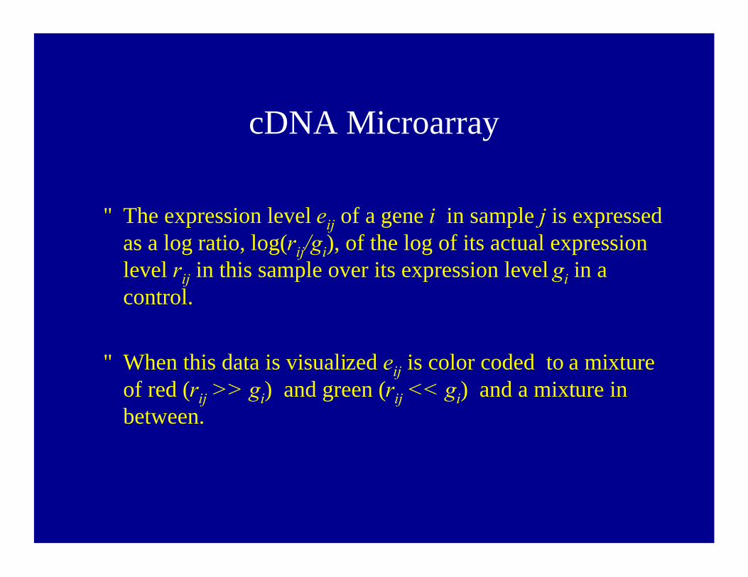
cDNA Microarray
• The expression level eij of a gene i in sample j is expressed as a log ratio, log(rij/gi), of the log of its actual expression level rij in this sample over its expression level gi in a control.
• When this data is visualized eij is color coded to a mixture of red (rij >> gi) and green (rij << gi) and a mixture in between.

Nylon Membrane and Plastic Arrays (by Clontech)
• A raw intensity and a background value are measured for each gene.
• The analyst is free to choose the raw intensity or can adjust it by subtracting the background intensity.

Oligonucleotide Silicon Chips (by Affymetrix)
• These arrays produce a variety of numbers derived from 16-20 pairs of perfect match (PM) and mismatch (MM) probes.
• There are several statistics related to gene expression that can be derived from this data. The most commonly used one is the average difference (AVD), which is derived from the differences of PM-MM in the 16-20 probe pairs.
• The next most commonly used method is the log absolute value (LAV), which comes from the ratios PM/MM in the probe pairs.
• Note: The Affymetrix gene-chip software has a absent/present call for each gene on a chip. According to Jagota, the method is complex and arbitrary so they usually ignore it.

For What Do We Use Microarray Data?• Genes with similar expression patterns over all samples –
We can compare the expression patterns ei and ei’ of two genes i and i' over all samples.
• If we use cluster analysis, we can separate the genes into groups of genes with similar expression patterns (trees).
• This will allow us to find what unknown genes have altered expression in a particular disease by comparing the pattern to genes know to be affiliated with a disease.
• It can also find genes that fit a certain pattern such as a particular pattern of change with time.
• It can also characterize broad functional classes of new genes from the known classes of genes with similar expression.

For What Do We Use Microarray Data?
• Genes with unusual expression levels in a sample – In contrast to standard statistical methods where we ignore outliers, here outliers might have particular importance. Hence, we look for genes whose expression levels are very different from the others.
• Genes whose expression levels vary across samples – We can compare gene expression levels of a particular gene or set of genes in different samples. This can be used to look compare normal and diseased tissues or diseased tissue before and after treatment.

For What Do We Use Microarray Data?
• Samples that have similar expression patterns – We might want to compare the expression patters of all genes between two samples. We might cluster the genes into gene with similar expression patterns to help with the comparison. This can be used to look compare normal and diseased tissues or diseased tissue before and after treatment.
• Tissues that might be cancerous (diseased) – We can take the gene expression pattern of sample and compare it to library expression patterns that indicate diseased or not diseased tissue.

Statistical Methods Can Help
• Experimental Design – Since using microarrays is costly and time consuming, we want to design experiments to use the minimal number of micorarrays that will give a statistically significant result.
• Data Pre-processing – It is sometimes useful to preprocess the data prior to visualization. An example of this is the log ratio mentioned earlier. It is often necessary to rescale data from different microarrays so that they can be compared. This is due to variation in chip to chip intensity. Another type of preprocessing is subtracting the mean and dividing by the variance.

Statistical Methods Can Help
• Data Visualization – Principle component analysis and multidimensional scaling are two useful techniques for reducing multidimensional data to two and three dimensions. This allows us to visualize it.
• Cluster Analysis – By associating genes with similar expression patterns, we might be able to draw conclusions about their functional expression.
• Probability Theory – We can use statistical modeling and inference to analyze our data. Probability theory is the basis for these.

Statistical Methods Can Help
• Statistical Inference – This is the formulation and statistical testing of a hypothesis and alternative hypothesis.
• Classifiers for the Data – We can construct classes from data, such a diseased vs. non-diseased tissue. We can build a model (such as a hidden Markov model) that fits know data for the different classes. This can then be used to classify previously unclassified data.

Preprocessing Microarray Data
• Before microarray data can be analyzed or stored, a number of procedures or transformations must be applied to it.
• In order to analyze the data correctly, it is important to understand what the transformations might be doing to the data.

Preprocessing Microarray Data• Ratioing the data• Log-tranforming ratioed data• Alternative to ratioing the data• Differencing the data• Scaling data across chips to account for chip-to-chip
difference• Zero-centering a gene on a sample expression pattern• Weighting the components of a gene or sample expression
pattern differently• Handling missing data• Variation filtering expression patterns• Discretizing expression data

Ratioing the data
• This is the most popular transformation. • The expression level eij of a gene i in sample j is expressed
as a ratio, (rij/gi), of its actual expression level rij in this sample over its expression level gi in a control.
• This tells us the level of under- or over- expression of a gene i in the sample j.
• If the control value gi is very small, it can make the ratio very big.
• This can skew results incorrectly.

Log-tranforming ratioed data
• This is also a popular transformation. • The expression level eij of a gene i in sample j is expressed
as a log ratio, log(rij/gi), of the log of its actual expressionlevel rij in this sample over its expression level gi in acontrol.
• This will suppress outliers caused when the control value gi
is very small. • However, it creates a new outlier when rij is very small.

An alternative that eliminated both of the outlier problems above is
This gives a value in [0,1] and can be interpreted at the probability of gene i is higher in sample j than in control.
Alternative to ratioing the data
iij
ij
grr+

Differencing the data
• Another transformation is to difference the data ie. rij – gi. • This is not really appropriate in our previous context. • However, this is used by Affymetrix in a different context. • In their data rij is the strength of the match of the target i to
a specific probe j and gi is he strength of the match of the target i to a control for this probe.

Scaling data across chips to account for chip-to-chip difference
• As mentioned previously, different chips might display different intensities.
• When comparing different chips the data might need to be scaled so that they are on the same scale.
• Alternatively, they can be normalized so that they are between [0,1] and compared.

Zero-centering a gene on a sample expression pattern
This in effect the same as subtracting the mean expression pattern.Suppose that x is an expression pattern for a particular gene giwhose components are log-ratios. Let where is the ‘average expression pattern’ or control. Then x indicates whether the gene gi is induced or repressed relative to control. (Remember the x’s are vectors).Subtracting the mean expression pattern and dividing by the standard deviation can accomplish this.
(Remember the x’s are vectors).
σxxx −
=′
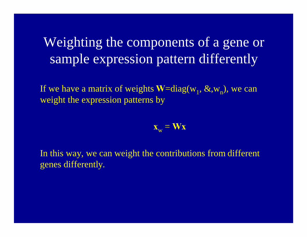
Weighting the components of a gene or sample expression pattern differently
If we have a matrix of weights W=diag(w1,…,wn), we can weight the expression patterns by
xw = Wx
In this way, we can weight the contributions from different genes differently.

Handling missing data
• Sometimes components of an expression pattern x are missing.
• To fix this, the missing values can be replaced by the mean over the non-missing values in x.

Variation filtering expression patterns
• When we are performing cluster analysis on gene or sample expression patterns, patterns with low variance will all seem sufficiently similar to each other and might form a cluster.
• This cluster will probably not reflect any interesting result.

Discretizing expression dataSometimes we might want to convert gene or sample expression pattern into discrete values. For example, if we have log-ratio, we may want to simply look at whether something is up- or down-regulated. To do this, we can do the following:
In this case +1 would indicate up-regulation, 0 would indicate no change and –1 would indicate down-regulation.
=<−>+
==000101
)( ,,
i
i
i
ibibb
xwhenxwhenxwhen
xwherexx
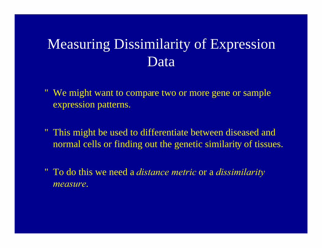
Measuring Dissimilarity of Expression Data
• We might want to compare two or more gene or sample expression patterns.
• This might be used to differentiate between diseased and normal cells or finding out the genetic similarity of tissues.
• To do this we need a distance metric or a dissimilarity measure.

Example Distance MetricEuclidean Distance – This is the most common distance measure.
This should not be used if either 1) Not all components of the vectors being compared have equal weight.2) There is missing data.Preprocessing the data can often alleviate these problems.We can also use the normalized Euclidean distance
n
yxyxd i
ii∑ −=
2)(),(
∑ −=i
ii yxyxd 2)(),(

Example Dissimilarity Measures
• Maximum Coordinate Difference – The following computes the maximum absolute distance along a coordinate
• Dot Product –This is a dissimilarity version of the dot product.
||max),( iiiyxyxd −=
yxyxd o−=),(
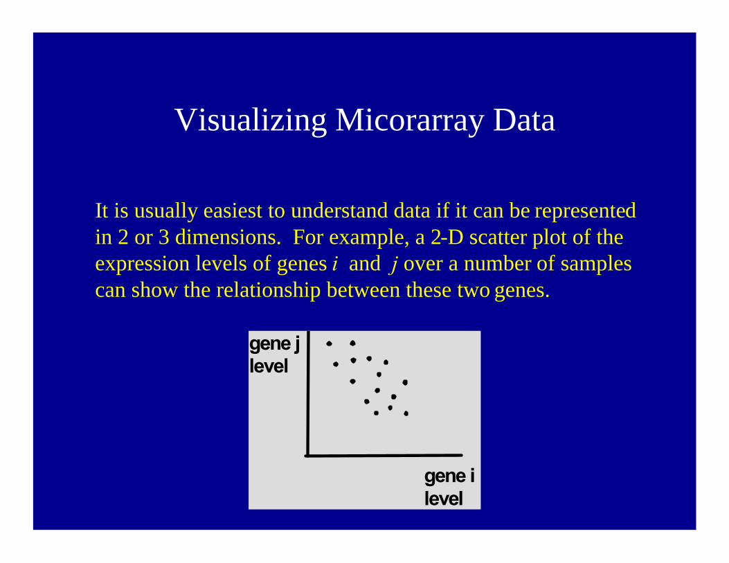
Visualizing Micorarray Data
It is usually easiest to understand data if it can be represented in 2 or 3 dimensions. For example, a 2-D scatter plot of the expression levels of genes i and j over a number of samples can show the relationship between these two genes.
gene jlevel
gene ilevel

Principal Components Analysis
• In principal components analysis n-dimensional data isconverted to d-dimensional data (d<<n) such that thecomponents in the new space are uncorrelated and axis ordimensions of the new space are ordered with respect to the amount of variance they explain.
• The first component explains the most about the data. • The second component is orthogonal to the first and
explains more about the data and so on.

Principal Components AnalysisExample – Consider height and weight data for a group of individuals. This is 2-D data, but there is a correlation between height and weight. We can use this property to reduce the data to 1D. PC1 explains most of the data and PC2 explains the rest.
height
weight
PC 1PC 2
PCA and Microarrays
Sample Application 1 – If we want to compare the sample expression patterns from two groups (diseased vs normal, experimental vs control). If we have n genes, the each pattern is a point in n-dimensional space. Suppose we want to see if the sample expression patterns for these two groups cluster by group. We might want to perform PCA analysis and perform cluster analysis at the top three components.

PCA and Microarrays
Sample Application 2 – On gene chips (such as the one made by Affymetrix), the same gene occupies multiple cells. In theory, the expression level of all cells with the same gene should be perfectly correlated. However, in practice, this is often not the case due to imperfections in the technology or hybridization of the sequence fragment to other genes in the target.

PCA and Microarrays
PCA allows us to see how good the correlation among these cells is. To use PCA, we would hybridize k different samples on the same chip. For each sample, the expression levels of a gene x in the n cells is an n-dimensional vector. Hence, there are k points in n-dimensional space. Using PCA, if most of the variance is explained by the first principal component, the effective dimensionality of the data is 1 and there cells are highly correlated.

PCA Limitations
• Clustering by PCA effectively yields clusters as if the Euclidean distance metric had been used. Hence, it is possible that it might miss clusters.
• The reduction of dimensionality uses all coordinates. If only a few genes out of a thousand differ between two samples (Application 1), clustering by PCA might not yield any meaningful results.

Cluster Analysis of Microarray Data
Recall that microarray data can be thought of as gene expression patterns or sample expression patterns. These can be each considered to be vectors. The first thing we have to do before applying cluster analysis is to find a distance between the various expression pattern vectors. This is done using similarity/dissimilarity measures such as Euclidean distance, Mahalonobis distance, or linear correlation coefficients. Once a distance matrix is computed, the following clustering algorithms can be used. The clusters formed can differ significantly depending upon the distance measure used.

Cluster Analysis of Microarray Data
Hierarchical Clustering – Assume each data point is in a singleton cluster.
Find the two clusters that are closest together. Combine these to form a new cluster.
Compute the distance from all clusters to the new cluster using some form of averaging.
Find the two closest clusters and repeat.

Cluster Analysis of Microarray Data
k-Means Clustering – An alternate method of clustering called k-means clustering, partitions the data into k clusters and finds cluster means µi for each cluster. In our case, the means will be vectors also.
Usually, the number of clusters k is fixed in advance. To choose k something must be know about the data. There might be a range of possible k values.
To decide which is best, optimization of a quantity that maximizes cluster tightness ie. minimizes distances between points in a cluster.

Cluster Analysis of Microarray Data
Self-organizing Maps – This is basically an application of neural networks to microarray data. Assume that there is a 2-dimensional grid of cells and a map from a given set of expression data vectors in Rn, ie, there are n nodes in the input layer and a connection neuron from each of these to each cell. Each cell (i, j) gets it own weight from n input neurons. The weight vector µij is the mean of the cluster associated with cell (i, j). Each data vector d gets mapped to the cell (i, j) that is closest to d using Euclidean distance.In order to train the network, the mean vectors µij for the cells (i, j) must be learned.

Hidden Markov Models and MicroarrayData
We can use Hidden Markov models for pattern recognition in the study of micorarray data. Suppose that we want to consider gene expression data from a tissue sample and want to know if it is control or different from the control (diseased, experimentally altered, responding to drug, etc.). Consider the gene expression data vector as a set of emissions, one for each vector coordinate. Each emission has a value that is defined by some probability distribution function. This can be continuous, or can even discrete. To make it discrete, the data should be preprocessed to indicate, up-regulation, down-regulation, or no significant change.

Finding Genes Expressed Unusually Different in a Population
The following section addresses the question: Is gene g expressed unusually in the sample?
The first thing to do is to come up with a formal mathematical definition for what unusual is. Assume that the microarray data is log transformed ratio data. If a histogram is constructed of the data, it should yield roughly a normal distribution. Anything that is out near either tail can be considered to be unusually expressed. Note that this can be either a high or low expression level.

Finding Genes Expressed Unusually Different in a Population
Calculate the Z-score for the data point considered
where eg is the expression level, µ is the mean and σ is the standard deviation. The Z value will give an indication of the how far the data is toward the tail (α - level).
Use statistical inference (hypothesis testing).
σµ−
= geZ