Lecture 1

Course: Numerical Solution of Ordinary Differential Equations

Module1: Numerical Solution of Ordinary Differential Equations

Lecture Content Hours

1 Solution of first order ordinary differential equations

Approximate Solution: Picard Iteration Method, Taylor Series method

1

2 Numerical Solution: Euler method; Algorithm; Example; analysis 1

3 Modified Euler Method: Algorithm; Example; analysis 1

4 Runge Kutta methods, Second Order methods 1

5 Fourth Order Runge Kutta methods 1

6 Higher Order Runge Kutta methods 1

References:

Bradie B A Friendly Introduction to Numerical Anaysis Pearson Education,2007

Burden RL, Faires J D Numerical Analysis Cengage Learning, 2007

Chapra SC, Canale, R P Numerical Methods for Engineers Tata McGraw Hill, 2003

Gerald C.F., Wheatley P O Applied Numerical analysis, Addison Wesley, 1998


Lecture 1

Numerical solution of first order ordinary differential equations

Keywords: Initial Value Problem, Approximate solution, Picard method, Taylor series

Solution of first order ordinary differential equations

Consider y(t) to be a function of a variable t. A first order Ordinary differential

equation is an equation relating y, t and its first order derivatives. The most general

form is :

F(t,y(t),y (t)) 0

The variable y is known as a dependent variable and t is independent variable. The

equation is of first order as it is the order of highest derivative present in the equation.

Sometimes it is possible to rewrite the equation in the form

y (t) f(t,y(t)) (1.1)

y g(t) is a solution of the first order differential equation (1.1) means

i) y(t) is differentiable

ii) Substitution of y(t) and y (t) in (1.1) satisfies the differential equation

identically

The differential equations are commonly obtained as mathematical representations of

many real world problems. Then the solution of the underlying problem lies in the

solution of differential equation. Finding solution of the differential equation is then

critical to that real world problem.

Examples of first order differential equations are:

y 2y 0

y siny exp(t)

The first of these equations represents the exponential decay of radioactive material

where y represent the amount of material at any given time and k=2 is the rate of decay.

It may be noted that y(t) c exp( 2t) is the solution of differential equation as it

identically satisfies the given differential equation for arbitrarily chosen constant c. This

means that the differential equation has infinitely many solutions for different choices of

c. In other words, the real world problem has infinitely many solutions which we know is

not true. In fact, an initial condition should be specified for finding the unique solution of

the problem:

y(0) A

That is, the amount of radioactive material present at time t=0 is A. When this initial

condition is imposed on the solution, the constant c is evaluated as A and the solution

y(t) A exp( 2t) is now unique. The expression can now be used for computing the

amount of material at any given time.

The solution with arbitrary constant is known as the general solution of the differential

equation. The solution obtained using the initial condition is a particular solution.

A first order Initial Value Problem (IVP) is defined as a first order differential equation

together with specified initial condition at t=t0:

There exist several methods for finding solutions of differential equations. However, all

differential equations are not solvable. The following well known theorem from theory of

differential equations establishes the existence and uniqueness of solution of the IVP:

Let f(t,y(t)) be continuous in a domain D={ (t,y(t)): t0≤t≤b, c≤y≤d } R2. If f satisfies

Lipschitz condition on the Variable y and (t0,y0) in D, then IVP has a unique solution

y=y(t) on the some interval t0 ≤ t ≤ t0+δ.

{The function f satisfies Lipschitz condition means that there exists a positive constant L

such that f(t,y) f(t,w) L y w }

The theorem gives conditions on function f(t, y) for existence and uniqueness of the

solution. But the solution has to be obtained by available methods. It may not be

possible to obtain analytical solution (in closed form) of a given first order differential

equation by known methods even when the above theorem guarantees its existence.

0 0 0y f(t,y); t t b with y(t ) y (1.2)

Sometimes it is very difficult to obtain the solution. In such cases, the approximate

solution of given differential equation can be obtained.

Approximate Solution

The classical methods for approximate solution of an IVP are:

i) Picard Iteration method

ii) Taylor Series method

Picard Iteration Method:

Picard method is an iterative method. An iterative method gives a sequence of

approximations y1(x), y2(x), …,yk(x),…to the solution of differential equations such that

the nth approximation is obtained from one or more prevoius approximations.

The integration of differential equation (1.2) yields

0

0

t

t

y(t) y f(x,y(x))dx

Note that the exact solution of IVP is obtained for t=t0

For approximate solution, the exact solution y(x) is approximated by y0 in the integrand

to get

1 0 0

0

t

t

y(t) y (x) y f(x,y )dx

The approximation can be improved as

2 0 1

0

t

t

y (x) y f(x,y )dx

A sequence of approximations y1(x), y2(x), …,yk(x),…can be obtained as

k 1 0 k

0

t

t

y (x) y f(x,y )dx ; k 0,1,2,...

(1.3)

From the theory of differential equations, it can be proved that the above sequence of

approximations converges to the exact solution of IVP.

Example 1.1: Obtain the approximate solution of IVP using Picard method. Obtain its

exact solution also

y 1 ty; y(0) 1

Solution: Given that y0=1. Using (1.3) gives

k 1 k k k

k 1 k k

t

0t t

0 0

y (t) 1 f(x,y )dx f(x,y ) 1 xy

y (t) 1 (1 xy )dx 1 t (xy )dx

Simplification yields the sequence of approximations as

21y (t) 1 t t / 2

t2 2 3 4

2

0

y (t) 1 t x(1 x x / 2)dx 1 t t / 2 t / 3 t / 8

t2 3 4

3

0

2 3 4 5 6

y (t) 1 t x(1 x x / 2 x / 3 x / 8)dx

1 t t / 2 t / 3 t / 8 t /15 t / 48

and so on.

The differential equation in example 1.1 is a linear first order equation. Its exact solution

can be obtained as

t2 2

0

y(t) exp(x / 2)[1 exp( x )dx]

The closed form solution of differential equation in this case is possible. But the

expression involving an integral is difficult to analyze. The sequence of polynomials as

obtained by Picard method gives only approximate solution, but for many practical

problems this form of solution is preferred.

Taylor Series method:

The IVP gives the solution y0 at initial point t=t0. for given step size h, the solution at

t=t0+h can be computed from Taylor series as

2 3

1 0 0 0 0 0

h hy(t ) y(t h) y(t ) hy (t ) y (t ) y (t ) ... (1.4)

2 6

From the differential equation, it is observed that

0 0 0 0 0y (t ) f(t ,y(t )) f(t ,y )

Repeated differentiation gives 0 0y (t ),y (t ),... as

0

2 22

0 2

0

0

t t

t t

f fyy (t )

t y

f f fy (t ) and so on2 y ( y )

t y yt

Substituting these derivatives and truncating the series (1.4) gives the approximate

solution at t1.

Example 1.2: Obtain the approximate solution y(t) of IVP using Taylor series method.

Obtain approximate solution at t= 0.1 correct to 4 places of decimal.

y 1 ty; y(0) 1

Solution: Given that y 1 ty f(t,y)

Repeated differentiations yield

iv

y y ty

y 2y ty

y (2y 1)y xy y and so on

Or ivy(0) 1, y (0) 1, y (0) 1, y (0) 2, y (0) 3,...

Substitution in (1.4) with t0=0 and h=t gives

2 3 4y(t) y(0 t) 1 t t / 2 t / 3 t / 8 ...

Taking t=0.1 and substitution in the above series gives

y(0.1) 1 0.1 0.01/ 2 0.001/ 3 0.0001/ 8 ....

Or y(0.1) 1 0.1 0.005 0.00033 0.0000125 ..

It may be noted that fifth term and subsequent terms are smaller than the accuracy

requirement, the Taylor series can be truncated beyond fourth term. Accordingly

y(0.1)=1.1.53.

Observe that the Picard method involves integration while Taylor series method

involves differentiation of the function f. Depending on the ease of operation, one can

select the appropriate method for finding the approximate solution. The number of

iterations in Picard method depends upon the accuracy requirement. The step size h

can be chosen sufficiently small to meet the accuracy requirement in case of Taylor

series method. For fixed h, more terms have to be included in the solution when more

accuracy is desired.

In the category of methods that include Picard method and Taylor series method, the

approximate solution is given in the form of a mathematical expression.


Lecture 2

Numerical Methods: Euler method

Keywords: Numerical solution, grid points, local truncation error, rounding error

Numerical Solution

Numerical methods for solving ordinary differential equations are more popular due to

several reasons:

More computational efforts are involved in Picard and Taylor series methods for

complex real life applications

Easy availability of computers

The numerical methods can still be applied in cases where the closed form

expression for the function is not available, but the values of function f are known

at finitely many discrete points. The analytical methods are not applicable.

For example, the velocity of a particle is measured at given points and one is interested

to predict the position of particle at some times in future. In such cases the analytical

methods cannot be applied and one has to obtain solution by numerical methods.

In this lecture a very basic method known as Euler method is being discussed. The

method is illustrated with an example.

Euler method:

When initial value problem (1.2) is solved numerically, the numeric values of the

solution y=g(t) are obtained at finitely many (say n) discrete points in the interval of

interest. Let these n points be equi-spaced in the interval [t0, b] as 1 2 nt , t ,..., t such that

0t kh, k 1,2,...n . These points are known as grid points. Here the step size h is

computed as 0b th

n

. The numeric value of the solution is known at t=t0. The

approximate numeric value yk of the solution at kth grid point t=tk is an approximation to

the exact solution y(tk) of IVP. The Euler method specifies the formula for computing the

solution:

k 1 k k ky y h f(t ,y ); k 0,1,2,...n 1 (1.5)

Fig1.1 Schematic Diagram for Euler Method

The Euler formula (1.5) is a one step difference formula. The solution obtained by this

formula is shown on the computational grid in figure 1.1.

Observe that 0 0 0f(t,y ); y(t ) y is the slope of the solution curve at t=t0. The solution is

approximated as a straight line passing through y (t0) = y0 having slope f(t0, y(t0)). The

actual solution y(t) (shown in blue) may not be a straight line and y(t1) may be different

than y1 computed by the formula (1.5). It is only an approximation to the exact solution.

Starting from this approximation y1 at t1, the solution at next grid point t2 can be

approximated as y2 using (1.5). This is further continued for other grid points.

The actual solution curve may be above/ below the approximated solution.

Accordingly, the algorithm for computing solution using Euler method is given below:

Algorithm 1 For numerical solution by Eulers method

Step 0 [initialization] k=0, h=(b-t0 )/n , y(tk)=yk,

Step 1 [computation] k 1 k k ky y h f(t ,y )

Step 2 [increment] tk+1=tk+h, k=k+1

t1

y(t)

t t2 tn‐1 tn

y1

y2

y0

Step 3 [check for continuation] If k< n go to step 1

Step 4 [termination] stop

Example 1.3: Solve the initial value problem using the above algorithm

3y t y; y(0) 1

The IVP is solved first for step size h=1. The solution is obtained at t=1, 2 and 3.

The computations are performed using MS-Excel diff-euler1.xls [See columns B and C.

The column D gives the truncation error.] Note that the equation can be solved exactly.

Its exact solution is y(t) 4exp( t / 3) t 3 , y(3.0)=1.471518.

Next, the same problem is solved with step size h=0.5 up to t=3. The solution is

obtained successively at t=0.5, 1.0, 1.5, 2.0, 2.5, 3.0. [See columns E and F of the same

MS-Excel sheet. The column G gives the error.]

Comparing y computed at t=3.0 by two different step sizes, it is observed that solution

with smaller step size is closer to exact solution.

The computations are repeated with step size h=0.25 and 0.125 also. [See the excel

sheet columns H to M. The column O of the sheet gives exact solution at grid points

with h=0.125].

The table 1.1 shows the application of Euler Method for h=0.125. The attached graph

shows that the difference between the exact solution and the solution obtained by Euler

method with h=0.125. The following conclusions can be drawn:

i) As step size decreases, the computational effort increases

ii) The accuracy of the approximate solution increases with decreasing step size

tk yk exact sol error

0 1 1 0

0.125 0.9583333 0.961758 -0.00342

0.25 0.9236111 0.930178 -0.01351

0.375 0.895544 0.904988 -0.00944

0.5 0.8738546 0.885927 -0.01207

0.625 0.8582774 0.872745 -0.01447

0.75 0.8485575 0.865203 -0.01665

0.875 0.8444509 0.86307 -0.01862

1 0.8457238 0.866125 -0.0204

1.125 0.852152 0.874157 -0.02201

1.25 0.8635206 0.886963 -0.02344

1.375 0.8796239 0.904347 -0.02472

1.5 0.9002646 0.926123 -0.02586

1.625 0.9252536 0.952111 -0.02686

1.75 0.9544097 0.982141 -0.02773

1.875 0.9875593 1.016046 -0.02849

2 1.024536 1.053668 -0.02913

2.125 1.0651803 1.094857 -0.02968

2.25 1.1093395 1.139466 -0.03013

2.375 1.156867 1.187356 -0.03049

2.5 1.2076225 1.238393 -0.03077

2.625 1.2614716 1.292448 -0.03098

2.75 1.3182853 1.349399 -0.03111

2.875 1.3779401 1.409126 -0.03119

3 1.4403176 1.471518 -0.0312

Table1.1: Solution of Example 1.3 with h=0.125

Observe that the error is increasing with t.

Fig 1.2: Comparison with exact solution (Example 1.3)

For the derivation of Euler formula, consider the finite difference approximation of the

derivative

k 1 k

kt t

y ydyhdx

Also the approximate value of the function f(t,y(t) is computed as

k k f(t,y(t)) f(t , y )

Substitution in the differential equation gives the Euler formula

k 1 k k ky y h f(t ,y )

When k=0, the right side of the formula can be computed from known initial value y0.

Once y1 is computed, other yk, k=2, 3, 4,… can be computed successively in the similar

manner.

Analysis :

The Taylors Theorem gives

2

k k k k k

hy(t h) y(t ) hy (t ) y ( ), (t ,t h)

2

yk

exact sol

Substituting the derivative from the differential equation and neglecting second order

terms of the Taylor theorem gives Euler formula which is an approximation of the

solution at next grid point:

k k k k

k 1 k k k

y(t h) y(t ) h f(t ,y(t ))

y y hf(t ,y )

Starting from the initial condition at t0, the approximate solution y1 at t1 computed by

Euler method has error due to following reasons:

i) The solution is assumed to be of constant slope equal to f(t0,y0) in the interval

(t0,t1)

ii) Rounding errors in numerical computation of the formula.

The local truncation error k 1 k k 1T y t h y is the difference between the exact

solution and approximate solution as obtained by the numerical method assuming the

solution is exact at kth step.

k 1 k k 1

2

k 1 k k k k k

2

k 1 k k k k k k

T y t h y

hT y(t ) h y (t ) y ( ) [y h f(t ,y )]

2

hT y(t ) y h[f(t ,y(t )) f(t ,y )] y ( )

2

Using the inequalities

k k k k k kf(t ,y(t ) f(t ,y ) L (y(t ) y ) and y ( ) M

the above expression for truncation error is simplified to

2

k 1 k

hT (1 hL) T M

2

For y1, the initial condition y0 is assumed to be the correct solution; hence the local

truncation error is of order h2.

However, the solution at t2 has one more source of error and that is approximate value

of the solution y1 at t1 as computed in earlier step. This error is further accumulated as

solution is advanced to more grid points tk, k=3, 4,… . The accumulation of error is

evident from the fig. 1.1 also. The Final Global Error (F.G.E) in computing the final value

at the end of the interval (a,b); a= t0, b=to+Mh is accumulated error in M steps and is of

order h. This means that the error E(y(b),h) in computing y(b) using step size h is

approximated as

( ( ), )E y B h Ch

Accordingly, ( ( ), / ) /E y B h 2 Ch 2

Therefore, halving the step size will half the FGE. FGE gives an estimate of

computational effort required to obtain an approximation to exact solution.

Repeated application gives

k 1

k 1

MhT 1 hL 1

2L

Using m mx0 (1 x) e ; x 1 gives overall truncation error of order h:

( )

k 1 hLk 1

MhT e 1

2L

Apart from the Euler method, there are numerous numerical methods for solving IVP. In

the next couple of lectures more methods are discussed. These are not exhaustive. The

selection of methods is based on the fact that these are generally used by scientists and

engineers in solving IVP because of their simplicity. Also, more complex techniques are

the combination of one or more of these and their development is on similar lines.


Lecture 3

Modified Euler Method

Keywords: Euler method, local truncation error, rounding error

Modified Euler Method: Better estimate for the solution than Euler method is expected

if average slope over the interval (t0,t1) is used instead of slope at a point. This is being

used in modified Euler method. The solution is approximated as a straight line in the

interval (t0,t1) with slope as arithmetic average at the beginning and end point of the

interval.

Fig1.3 Schematic Diagram for Modified Euler Method

Accordingly, y1 is approximated as

0 1 0 0 1 11 1 0 0

(y + y ) (f(t ,y(t )+ f(t ,y(t ))y(t ) y = y +h y +h

2 2

However the value of y( t1) appearing on the RHS is not known. To handle this, the

value of y1p is first predicted by Euler method and then the predicted value is used in

(1.6) to compute y1’ from which a better approximation y1c to y1 can be obtained:

1,p 0 0 0y y h f(t ,y );

0 0 1 1,p

1c 0

f(t ,y ) f(t ,y )y y h

2

The solution at tk+1 is computed as

k 1,p k k ky y h f(t ,y ) ;

k k k 1 k 1,pk 1 k


2

In the fig (1.3), observe that black dotted line indicates the slope f(t0,y(t0)) of the solution

curve at t0, red line indicates the slope f(t1,y(t1)), at the end point t1. Since the solution at

end point y(t1) is not known at the moment, its approximation y1p as obtained from Euler

y1c

y1p

t0 t1

y0

method is used. The blue line indicates the average slope. Accordingly, y1 is a better

estimate than y1p. The method is also known as Heun’s Method.

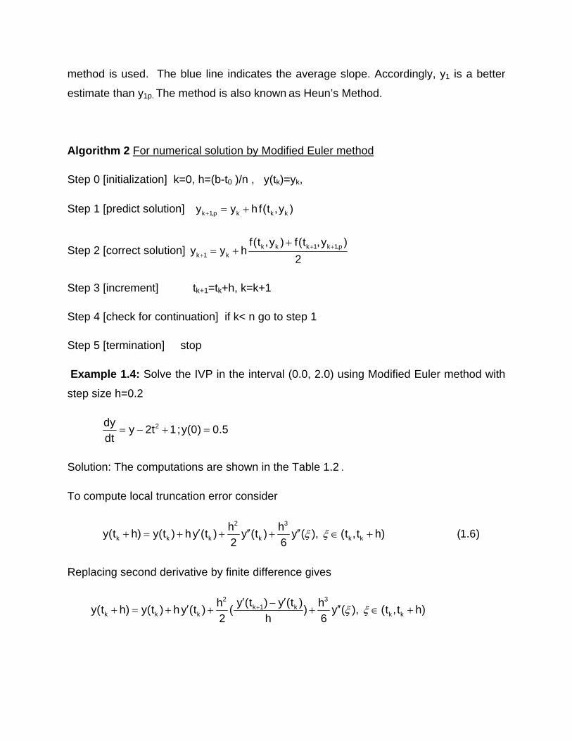
Algorithm 2 For numerical solution by Modified Euler method

Step 0 [initialization] k=0, h=(b-t0 )/n , y(tk)=yk,

Step 1 [predict solution] k 1,p k k ky y h f(t ,y )

Step 2 [correct solution] k k k 1 k 1,pk 1 k


2

Step 3 [increment] tk+1=tk+h, k=k+1

Step 4 [check for continuation] if k< n go to step 1

Step 5 [termination] stop

Example 1.4: Solve the IVP in the interval (0.0, 2.0) using Modified Euler method with

step size h=0.2

2dyy 2t 1;y(0) 0.5

dt

Solution: The computations are shown in the Table 1.2 .

To compute local truncation error consider

2 3

k k k k k k

h hy(t h) y(t ) hy (t ) y (t ) y ( ), (t ,t h) (1.6)

2 6

Replacing second derivative by finite difference gives

2 3k 1 k

k k k k k

y (t ) y (t )h hy(t h) y(t ) hy (t ) ( ) y ( ), (t ,t h)

2 h 6

Further simplification gives local truncation error of modified Euler formula as O(h3):

3

k k k k 1 k k

h hy(t h) y(t ) ( y (t ) y (t )) y ( ), (t ,t h)

2 6

The FGE in this method is of order h2. This means that halving the step size will reduce

the error by 25%.

Table 1.2 Modified Euler Method Example 1.4

[Reference excel sheet modified-euler.xlsx ]

The Euler method and Modified Euler methods are explicit single step methods as they

need to know the solution at a single step. It may be observed that the Euler method is

derived by replacing derivative by forward difference:

( )

k

k 1 k

t t

y ydyO h

dt h

The central and backward difference approximation can also be used to give single step

methods

( )

k

k k 1

t t

y ydyO h

dt hor ( )

k

2k 1 k 1

t t

y ydyO h

dt 2h

t y0 f(t0,y0) t1 y1p f(t1,y1p) y1c

0 0.5 1.5 0.2 0.8 1.72 0.822

0.2 0.822 1.742 0.4 1.1704 1.8504 1.18124

0.4 1.18124 1.86124 0.6 1.553488 1.833488 1.550713

0.6 1.550713 1.830713 0.8 1.916855 1.636855 1.89747

0.8 1.89747 1.61747 1 2.220964 1.220964 2.181313

1 2.181313 1.181313 1.2 2.417576 0.537576 2.353202

1.2 2.353202 0.473202 1.4 2.447842 -0.47216 2.353306

1.4 2.353306 -0.56669 1.6 2.239967 -1.88003 2.108634

1.6 2.108634 -2.01137 1.8 1.70636 -3.77364 1.530133

1.8 1.530133 -3.94987 2 0.740159 -6.25984 0.509162

2 0.509162 -6.49084 2.2 -0.78901 -9.46901 -1.08682

Module1

Numerical Solution of Ordinary Differential Equations

Lecture 4

Runge Kutta Method

Keywords: one step algorithm, Taylor series, Runge-Kutta method

Runge Kutta Method

The solution of differential equation with desired accuracy can be achieved using

classical Taylor series method at a specified point. This means for given h, one can go

on adding more and more terms of the series till the desired accuracy is achieved. This

requires the expressions for several higher order derivatives and its evaluation. It poses

practical difficulties in the application of Taylor series method:

Higher order derivatives may not be easily obtained

Even if the expressions for derivatives are obtained, lot of computational effort may

still be required in their numerical evaluation

It is possible to develop one step algorithms which require evaluation of first derivative

as in Euler method but yields accuracy of higher order as in Taylor series. These

methods require functional evaluations of f(t,y(t)) at more than one point.on the interval

[tk,tk+1]. The Category of methods are known as Runge-Kutta methods of order 2, 3 and

more depending upon the order of accuracy. .A general Runge Kutta algorithm is given

as

( , , )k 1 k k ky y h t y h (1.7)

The function phi is termed as increment function. The mth order Runge-Kutta method

gives accuracy of order hm. The function is chosen in such a way so that when

expanded the right hand side of (1.7) matches with the Taylor series upto desired order.

This means that for a second order Runge-Kutta mehod the right side of (1.7 ) matches

up to second order terms of Taylor series.

Second Order Runge Kutta Methods

The Second order Runge Kutta methods are known as RK2 methods. For the derivation

of second order Runge Kutta methods, it is assumed that phi is the weighted average of

two functional evaluations at suitable points in the interval [tk,tk+1]:

( , , )

( , )

( , ); ,

k k 1 1 2 2

1 k k

2 k k 1

t y h w K w K

K f t y

K f t ph y qhK 0 p q 1

(1.8)

Here, four constants w1, w2, p and q are introduced. These are to be chosen in such a

way that the expansion matches with the Taylor series up to second order terms.

For this

( , )

( , ) ( , ) ( , ) ( )

( , ) ( , ) ( , )( ( , ) ( )

2 k k 1

2k k t k k 1 y k k

2k k t k k k k y k k

K f t ph y qhK

f t y phf t y qhK f t y O h

f t y phf t y qhf t y f t y O h

(1.9)

Substitution in (1.7 ) yields

[ ( , ) { ( , ) ( , ) ( , )( ( , ) ( )}]2

k 1 k 1 k k 2 k k t k k k k y k ky y h w f t y w f t y phf t y qhf t y f t y O h

Or

[ ( , ) ( , )] [ ( , ) ( , )( ( , )] ( )2 3

k 1 k 1 k k 2 k k t k k k k y k ky y h w f t y w f t y h pf t y qf t y f t y O h (1.10)

Let us write the Taylor series for the solution y(tk+h) as

( ) ( ) ( ( )) ( , ( )) ( , ( ));2 3

k k k k k k k k

h hy t h y t hf t y t f t y t f y t t 1

2 6

Using chain rule for the derivative ( , ( ))k kf t y t gives

( , ( )) ( , ( )) ( , ( ))( ( , ( ))k k t k k k k y k kf t y t f t y t f t y t f t y t

Substituting in Taylor series gives

( ) ( ) ( ( )) [ ( , ( )) ( , ( ))( ( , ( ))] ( )2

3k k k k t k k k k y k k

hy t h y t hf t y t f t y t f t y t f t y t O h

2 (1.11)

Assuming ( )k ky t y and comparing (1.10) and (1.11) yields

, / /1 2 1 2w w 1 w p 1 2 and w q 1 2 (1.12)

Observe that four unknowns are to be evaluated from three equations. Accordingly

many solutions are possible for (1.12). Let us chose arbitrary value to constant q as

q=1, then

/ ,1 2w w 1 2 p 1 and q 1

Accordingly, the second order Runge-Kutta can be written as

( , )

[ ( , ) ( , )]

kp k k k

k 1 k k k k kp

y y hf t y

hy y f t y f t h y

2

(1.13)

This is the same as modified Euler method. It may be noted that the method reduces to

a quadrature formula [Trapezoidal rule] when f(t, y) is independent of y:

[ ( ) ( )] k 1 k k k

hy y f t f t h

2

For convenience q is chosen between 0 and 1such that one of the weights w in the

method is zero. For example choose q=1/2 makes w1=0 and (1.12) yields:

, , /1 2w 0 w 1 p q 1 2

( , )

( , )

k k k k

k 1 k k k

hy y f t y

2h

y y hf t y2

(1.14)

Choosing arbitrary constant q so as to minimize the sum of absolute values of

coefficients in the truncation error term Tj+1 gives optimal RK method. The minimum

error occurs for q=2/3. Accordingly optimal method is obtained for

/ , / , /1 2w 1 4 w 3 4 p q 2 3

This gives another second order Runge-Kutta method known as optimal RK2 method:

( , )

( , ) ( , )

k k k k

k 1 k k k k k

2hy y f t y

3h 3h 2h

y y f t y f t y4 4 3

(1.15)

Example 1.5: Solve IVP in 1<t<2 with h=0.1using Optimal Runge Kutta Method (1.15)

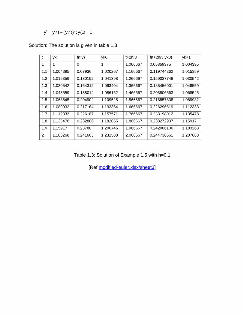
/ ( / ) ; ( ) 2y y t y t y 1 1

Solution: The solution is given in table 1.3

t yk f(t,y) yk0 t+2h/3 f(t+2h/3,yk0) yk+1

1 1 0 1 1.066667 0.05859375 1.004395

1.1 1.004395 0.07936 1.020267 1.166667 0.119744262 1.015359

1.2 1.015359 0.130192 1.041398 1.266667 0.159037749 1.030542

1.3 1.030542 0.164312 1.063404 1.366667 0.185456001 1.048559

1.4 1.048559 0.188014 1.086162 1.466667 0.203806563 1.068545

1.5 1.068545 0.204902 1.109525 1.566667 0.216857838 1.089932

1.6 1.089932 0.217164 1.133364 1.666667 0.226296619 1.112333

1.7 1.112333 0.226187 1.157571 1.766667 0.233198012 1.135478

1.8 1.135478 0.232886 1.182055 1.866667 0.238272937 1.15917

1.9 1.15917 0.23788 1.206746 1.966667 0.242006106 1.183268

2 1.183268 0.241603 1.231588 2.066667 0.244736661 1.207663

Table 1.3: Solution of Example 1.5 with h=0.1

[Ref modified-euler.xlsx/sheet3]


Lecture 5

Fourth Order Runge Kutta Methods

Keywords: fourth order methods, Taylor series, convergence, stability

Fourth Order Runge-Kutta Methods (RK4)

All the fourth order Runge Kutta Methods are of the following general form:

( , , )

( , )

( , )

( , )

( , )

k 1 k k k

1 1 2 2 3 3 4 4

1 k k

2 k 1 k 21 1

3 k 2 k 31 1 32 2

4 k 3 k 41 1 42 2 43 3

y y h t y h

w K w K w K w K

K f t y

K f t p h y a K

K f t p h y a K a K

K f t p h y a K a K a K

(1.16)

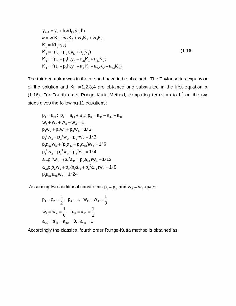
The thirteen unknowns in the method have to be obtained. The Taylor series expansion

of the solution and Ki, i=1,2,3,4 are obtained and substituted in the first equation of

(1.16). For Fourth order Runge Kutta Method, comparing terms up to h4 on the two

sides gives the following 11 equations:

; ;

/

/

( ) /

/

( ) /

( ) /

1 21 2 31 32 3 41 42 43

1 2 3 4

1 2 2 3 3 4

2 2 21 2 2 3 3 4

1 32 2 1 42 2 43 4

3 3 31 2 2 3 3 4

2 232 1 3 1 42 2 43 4

232 1 2 3 3 1 42 2 43 4

1 32

p a p a a p a a a

w w w w 1

p w p w p w 1 2

p w p w p w 1 3

p a w p a p a w 1 6

p w p w p w 1 4

a p w p a p a w 1 12

a p p w p p a p a w 1 8

p a a /43 4w 1 24

Assuming two additional constraints 1 2 2 3p p and w w gives

, ,

,

,

1 2 3 2 3

1 4 21 32

31 41 42 43

1 1p p p 1 w w

2 31 1

w w a a6 2

a a a 0 a 1

Accordingly the classical fourth order Runge-Kutta method is obtained as

[ ]

( , )

( , )

( , )

( , )

k 1 k 1 2 3 4

1 k k

2 k k 1

3 k k 2

4 k k 3

hy y K 2K 2K K

6K f t y

h hK f t y K

2 2h h

K f t y K2 2

K f t h y hK

(1.16)

It may be observed that RK4 uses four functional evaluations in the interval [ t0, t1].

These points are shown as p0, p1, p2 and p3 in the following figure

Fig1.4 Schematic Diagram for RK4 Method

Example 1.6: find the solution of IVP using classical fourth order Runge-Kutta method

with h=1

; ( )dy 1 y

y 1 0dt 2 t

Solution: The solution of IVP by RK4 classical method is shown in the following table:

h k tk yk k1 k2 k3 k4 yk+1 exact sol Abs error

1 0 1 0 0.5 0.66667 0.72222 0.861111 0.689815 0.693147 0.00333

1 1 2 0.68981 0.84491 0.94491 0.96491 1.051574 1.6425 1.647918 0.00542

1 2 3 1.6425 1.0475 1.11893 1.12913 1.192908 2.765255 2.772589 0.00733

1 3 4 2.76526 1.19131 1.24687 1.25304 1.303659 4.014388 4.023595 0.00921

1 4 5 4.01439 1.30288 1.34833 1.35246 1.394475 5.364212 5.375278 0.01107

1 5 6 5.36421 1.39404 1.4325 1.43546 1.471381 6.797766 6.810686 0.01292

1 6 7 6.79777 1.47111 1.50444 1.50666 1.538054 8.302995 8.317766 0.01477

1 7 8 8.303 1.53787 1.56729 1.56902 1.59689 9.87089 9.887511 0.01662

1 8 9 9.87089 1.59677 1.62308 1.62447 1.649536 11.49446 11.51293 0.01847

1 9 10 11.4945 1.64945 1.67326 1.67439 1.697168 13.16811 13.18842 0.02032

1 10 11 13.1681 1.6971 1.71884 1.71978 1.740658 14.88727 14.90944 0.02217

Table 1.4: Solution by Classical RK4 for example 1.6

[Reference R4_CLASSICAL.xlsx/sheet1]

Various entries of the table in a row are computed by the RK4 classical formula (1.16).

For computations in the table the user is referred to the excel sheet

R4_CLASSICAL.xlsx/sheet1

The solutions are compared with the exact solution and the absolute error is given in the

last column.

The other RK4 formulae are obtained as

[ ]

( , )

( , )

( , )

( , )

k 1 k 1 2 3 4

1 k k

2 k k 1

3 k k 1 2

4 k k 1 2 3

hy y K 3K 3K K

8K f t y

h hK f t y K

3 32h h

K f t y K hK3 3

K f t h y hK hK hK

(1.17)

and

[ ( ) ( ) ]

( , )

( , )

( , ( ) ( ) )

( , ( ) )

k 1 k 1 2 3 4

1 k k

2 k k 1

3 k k 1 2

4 k k 2 3

h 1 1y y K 2 1 K 2 1 K K

6 2 2K f t y

h hK f t y K

2 2h 1 1 1

K f t y hK 1 hK2 2 2 2

1 1K f t h y hK 1 hK

2 2

(1.18)

Example 1.7: find the solution of IVP using classical fourth order Runge-Kutta method

given in (1.17) with h=1

; ( )dy 1 y

y 1 0dt 2 t

Solution: In the following table the computation are shown to solve the IVP using (1.17).

Although both the methods are of same order but (1.17) gives more accurate result as

compared to classical method (1.16)

h k tk yk k1 k2 k3 k4 yk+1 exact sol Abs error

1 0 1 0 0.5 0.625 0.775 0.825 0.690625 0.693147 0.00252

1 1 2 0.69063 0.84531 0.91674 0.9971 1.038765 1.643824 1.647918 0.00409

1 2 3 1.64382 1.04794 1.09794 1.15249 1.186578 2.76705 2.772589 0.00554

1 3 4 2.76705 1.19176 1.23022 1.27143 1.300004 4.016642 4.023595 0.00695

1 4 5 4.01664 1.30333 1.33458 1.36767 1.392176 5.366922 5.375278 0.00836

1 5 6 5.36692 1.39449 1.4208 1.44843 1.469863 6.80093 6.810686 0.00976

1 6 7 6.80093 1.47156 1.49429 1.518 1.537026 8.306613 8.317766 0.01115

1 7 8 8.30661 1.53833 1.55833 1.5791 1.59619 9.874961 9.887511 0.01255

1 8 9 9.87496 1.59722 1.61508 1.63355 1.649065 11.49898 11.51293 0.01395

1 9 10 11.499 1.6499 1.66603 1.68266 1.696865 13.17308 13.18842 0.01534

1 10 11 13.1731 1.69755 1.71226 1.72738 1.74048 14.8927 14.90944 0.01674

Table 1.5 Solution By Classical RK4 for example 1.7

[Reference R4_CLASSICAL.xlsx/sheet2]

Let Tk+1(h) be the local truncation error at the( k+1)th step of the one step method with

step size h, assuming that no error was made in the previous step. It is obtained as

( ) ( , , ) k 1 k 1 k k kT h y y h t y h

The method is said to be consistent if

k 1

h 0

T (h)lim 0

h

It is now easy to verify that the Euler, Modified Euler and Runge-Kutta methods are

consistent

It is now easy to verify that the Eulers, Modified Eulers and Runge Kutta methods are

consistent.

A one step method is convergent when the difference between the exact solution and

the solution of difference equation at kth step satisfies the condition

k kh 0 1 k Nlim max y(t ) y 0

Using the bound for Tk=y(tk)-yk proves the convergence of Euler method.

Stability of a numerical method ensures that small changes in the initial conditions

should not lead to large changes in the solution. This is particularly important as the

initial conditions may not be given exactly. The approximate solution computed with

errors in initial condition is further used as the initial condition for computing solution at

the next grid point. This accounts for large deviation in the solution started with small

initial errors. Also round off errors in computations may also affect the accuracy of the

solution at a grid point. Euler method is found to be stable.

According to Lax equivalence theorem Given a properly posed initial value problem and

a finite-difference approximation to it that satisfies the consistency condition, stability is

the necessary and sufficient condition for convergence.


Lecture 6

Higher order Runge Kutta Methods

Keywords: higher order methods, functional evaluations, accuracy

Higher order Runge Kutta Methods

The local error of RK4 is O(h5) while the global error is O(h4). If the solution of IVP is to

be obtained for t in the interval (0,1] with h=0.1 using RK4, then the solution is to be

computed at 10 grid points t=0.1, 0.2, … ,1.0. At each grid point four functional

evaluations are required. This way, the solution at t=1 requires 40 functional evaluations

and the accuracy will be of order 10-4. If Euler method is to be used then h=0.0001 will

yield the desired accuracy of 10-4. Accordingly, the solution is to be computed at 10000

grid points to reach to t=1.This means Euler method requires10,000 functional

evaluations (one for each grid point) to compute approximate solution at t=1. Evidently,

RK4 is very efficient and saves lots of computational effort.

We can further improve the efficiency by employing still higher order Runge-Kutta

methods. The higher order methods, say of order 5 and 6 are developed on the same

lines. These are more efficient as the higher accuracy is achieved with less

computational effort as compared to lower order methods.

Runge-Kutta method ( say of order 4) is applied for obtaining approximate solution y1 at

t=t1=t+h for IVP with chosen value of h. The value of h is then halved and the solution is

again obtained at t1. Now 7 functional evaluations are needed to compute y1. If the

difference between two solutions is not substantial then the approximation is accepted.

Otherwise, the iteration (halving h) is repeated again till the desired accuracy is

achieved. Each halving h will require 4+7 functional evaluations. This way higher

accuracy can be achieved with more computational effort.

In another approach, higher performance with less computational effort is achieved

when the Runge-Kutta methods of different orders are used to move from one grid point

to the next point. One such method known as Runge-Kutta Fehlberg method is based

on the formulae (1.19) given below. In this, two estimates are obtained for yk+1 using RK

method of global error O(h4) and O(h5) with six functional evaluations.

( , )

( , )

( , )

( , )

( , )

( ,

1 k k

2 k k 1

3 k k 1 2

4 k k 1 2 3

5 k k 1 2 3 4

6 k k 1 2 3

K f t y

h hK f t y K

4 43h 3h 9h

K f t y K K8 32 32

12h 1932h 7200h 7296hK f t y K K K

13 2197 2197 2197439h 3680h 845h

K f t h y K 8hK K K216 513 4104

h 8h 3544hK f t y K 2hK K

2 27 2565

)

ˆ [ ]

[ ]

ˆ [ ]

4 5

k 1 k 1 3 4 5

k 1 k 1 3 4 5 6

k 1 k 1 1 3 4 5 6

1859h 11hK K

4104 40h 25 1408 2197 1

y y K K K K8 216 2565 4104 5h 16 6656 28561 9 2

y y K K K K K8 135 12825 56430 50 55

1 128 2197 1 2Error y y K K K K K h

360 4275 75240 50 55

(1.19)

Since the lower order method is of order four, the step size adjustment factor s can be

computed as

/

.

1 4

i 1

s 0 84T

Here, ε is the accuracy requirement and T is the truncation error ˆi 1 i 1 i 1T y y .

If the desired accuracy is not achieved the solution is iterated taking new value of h.

Depending upon error requirement the step size h can be increased or decreased. The

solution yk+1 of desired accuracy is obtained at tk+1=tk+sh. The method is known as

RKF45. To implement the method, the user specifies the allowable smallest step size

hmin , largest step size hmax and the maximum allowable local truncation error ε. The

following algorithm is used to solve IVP using RKF45 formulae with self adjusting

variable step sizes:

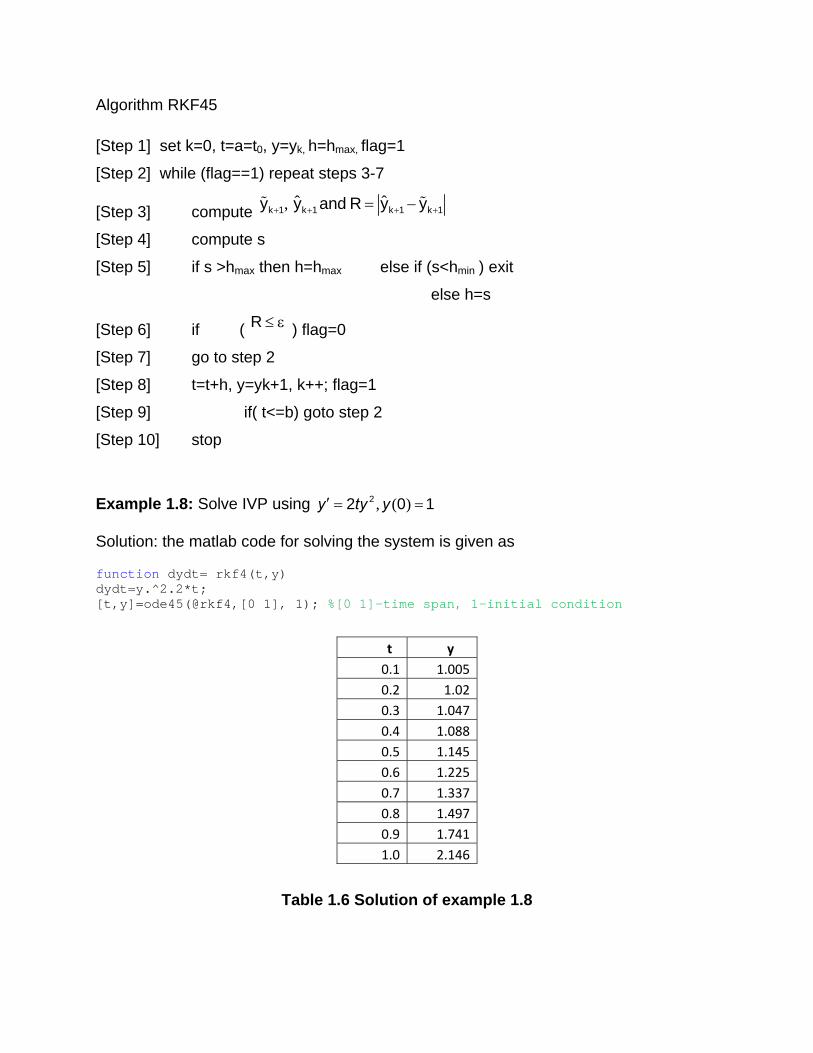
Algorithm RKF45

[Step 1] set k=0, t=a=t0, y=yk, h=hmax, flag=1

[Step 2] while (flag==1) repeat steps 3-7

[Step 3] compute ˆ ˆ,k 1 k 1 k 1 k 1y y and R y y

[Step 4] compute s

[Step 5] if s >hmax then h=hmax else if (s<hmin ) exit

else h=s

[Step 6] if ( R ) flag=0

[Step 7] go to step 2

[Step 8] t=t+h, y=yk+1, k++; flag=1

[Step 9] if( t<=b) goto step 2

[Step 10] stop

Example 1.8: Solve IVP using , ( )22 0 1y ty y

Solution: the matlab code for solving the system is given as

function dydt= rkf4(t,y) dydt=y.^2.2*t; [t,y]=ode45(@rkf4,[0 1], 1); %[0 1]-time span, 1-initial condition

Table 1.6 Solution of example 1.8

t y

0.1 1.005

0.2 1.02

0.3 1.047

0.4 1.088

0.5 1.145

0.6 1.225

0.7 1.337

0.8 1.497

0.9 1.741

1.0 2.146

Example 1.9: find the solution of IVP using higher order order Runge-Kutta method

RKF45 given in (1.19) in the interval (0,2) taking h max=0.25, hmin=0.01 and accuracy

as 0.000001

; ( ) .2dyy t 1 y 0 0 5

dt

Solution: The detailed solution of the problem is worked out in the excel sheet rkf45.xls

h t y k1 k2 k3 k4 k5 Kk6 y5 0.25 0 0.5 1.5 1.589844 1.638153 1.833988 1.863381 1.681916 0.92048705 0.188324 0 0.5 1.5 1.568405 1.604568 1.753716 1.775389 1.638313 0.80850123 0.25 0.188324 0.808501 1.773035 1.856403 1.901019 2.079976 2.10662 1.94126 1.2937217 0.192067 0.188324 0.808501 1.773035 1.83778 1.87192 2.011491 2.031676 1.903627 1.17405097 0.20392 0.380391 1.174051 2.029354 2.091427 2.124074 2.255372 2.274263 2.154073 1.61316482 0.206565 0.584311 1.613165 2.271745 2.326045 2.354349 2.465632 2.481366 2.380102 2.10457288 0.214212 0.790876 2.104573 2.479088 2.524275 2.54744 2.634325 2.646171 2.568076 2.6543036 0.225464 1.005088 2.654304 2.644102 2.676656 2.692615 2.74499 2.751256 2.706084 3.26380128 0.24762 1.230552 3.263801 2.749544 2.763568 2.768682 2.767586 2.764947 2.771299 3.94887292 0.25 1.478171 3.948873 2.763882 2.747947 2.735929 2.656062 2.640557 2.722156 4.62774423 0.25 1.728171 4.627744 2.641168 2.586313 2.552099 2.370792 2.338767 2.517156 5.25474897 0.206501 1.728171 4.627744 2.641168 2.596419 2.569447 2.430547 2.406828 2.541928 5.15141426 0.215663 1.934673 5.151414 2.408456 2.326784 2.278814 2.042876 2.003464 2.231007 5.63074392

Table 1.7 Details of Solution of example 1.9

Table 1.8 Comparison with exact Solution of example 1.9

tk+1 y5 exact tk+1 y5 exact 0.25 0.92048705 0.920487292 1.230552 3.26380128 3.263801766

0.188324 0.80850123 0.808501278 1.478171 3.94887292 3.948873499 0.438324 1.2937217 1.293721978 1.728171 4.62774423 4.62774482 0.380391 1.17405097 1.174051068 1.978171 5.25474897 5.254749428 0.584311 1.61316482 1.613164996 1.934673 5.15141426 5.151414894 0.790876 2.10457288 2.104573148 2.150336 5.63074392 5.6307445181.005088 2.6543036 2.654303965

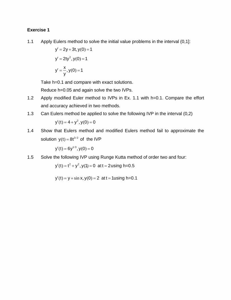
Exercise 1

1.1 Apply Eulers method to solve the initial value problems in the interval (0,1]:

, ( )y 2y 3t y 0 1

, ( )2y 2ty y 0 1

, ( )x

y y 0 1y

Take h=0.1 and compare with exact solutions.

Reduce h=0.05 and again solve the two IVPs.

1.2 Apply modified Euler method to IVPs in Ex. 1.1 with h=0.1. Compare the effort

and accuracy achieved in two methods.

1.3 Can Eulers method be applied to solve the following IVP in the interval (0,2)

( ) , ( )2y t 4 y y 0 0

1.4 Show that Eulers method and modified Eulers method fail to approximate the

solution /( ) 3 2y t 8t of the IVP

/( ) , ( )1 3y t 6y y 0 0

1.5 Solve the following IVP using Runge Kutta method of order two and four:

( ) , ( )2 2y t t y y 1 0 at t 2using h=0.5

( ) sin , ( )y t y x y 0 2 at t 1using h=0.1


Module 2: Multi-step methods


1 Single step and Multi-step methods, Predictor corrector methods, Milne’s method

2

2 Adams-Moulton method. 1

3 Adams Bashforth method 1

Module 2

Lecture 1

Multi Step Methods

Predictor corrector Methods

keywords: multi-step predictor, corrector, Milne-simpson method, integration formulae

Consider I VP

0 0 0y f(t,y); t t b with y(t ) y (2.1)

One step methods for solving IVP (2.1) are those methods in which the solution yj+1 at

the j+1th grid point involves only one previous grid point where the solution is already

known. Accordingly, a general one step method may be written as

j+1 j j jy =y +h (t ,y ,h)

The increment function Φ depends on solution yj at previous grid point tj and step size h.

If yj+1 can be determined simply by evaluating right hand side then the method is explicit

method. The methods developed in the module 1 are one step methods. These

methods might use additional functional evaluations at number of points between tj and

tj+1. These functional evaluations are not used in further computations at advanced grid

points. In these methods step size can be changed according to the requirement.

It may be reasonable to develop methods that use more information about the solution

(functional values and derivatives) at previously known values while computing solution

at the next grid point. Such methods using information at more than one previous grid

points are known as multi-step methods and are expected to give better results than

one step methods.

To determine solution yj+1, a multi-step method or k-step method uses values of y(t) and

f(t,y(t)) at k previous grid points tj-k, k=0,1,2,…k-1,. yj is called the initial point while yj-k

are starting points. The starting points are computed using some suitable one step

method. Thus multi-step methods are not self starting methods.

Integrating (2.1) over an interval (tj-k, tj+1) yields

j 1 j 1

j k j k

t t rj

j 1 j j jj 0t t

y y f(t,y(t))dt y a t dt

(2.2)

The integrand on the right side is approximated by interpolating polynomial of degree r

using equi-spaced points. The integration over the interval is shown in the Fig 2.1.

The method may be explicit or implicit. An implicit method involves computation of yj+1 in

terms of yj+1. First an explicit formula known as predictor formula is used to predict yj+1.

Then another formula, known as corrector formula, is used to improve the predicted

value of yj+1. The predictor-corrector methods form a large class of general methods for

numerical integration of ordinary differential equations. A popular predictor-corrector

scheme is known as the Milne-Simpson method.

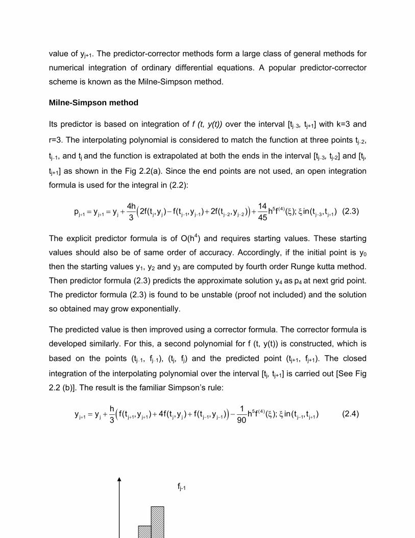
Milne-Simpson method

Its predictor is based on integration of f (t, y(t)) over the interval [tj−3, tj+1] with k=3 and

r=3. The interpolating polynomial is considered to match the function at three points tj−2,

tj−1, and tj and the function is extrapolated at both the ends in the interval [tj−3, tj-2] and [tj,

tj+1] as shown in the Fig 2.2(a). Since the end points are not used, an open integration

formula is used for the integral in (2.2):

5 (4)j 1 j 1 j j j j 1 j 1 j 2 j 2 j 3 j 1

4h 14p y y 2f(t ,y ) f(t ,y ) 2f(t ,y ) h f ( ); in(t ,t )

3 45 (2.3)

The explicit predictor formula is of O(h4) and requires starting values. These starting

values should also be of same order of accuracy. Accordingly, if the initial point is y0

then the starting values y1, y2 and y3 are computed by fourth order Runge kutta method.

Then predictor formula (2.3) predicts the approximate solution y4 as p4 at next grid point.

The predictor formula (2.3) is found to be unstable (proof not included) and the solution

so obtained may grow exponentially.

The predicted value is then improved using a corrector formula. The corrector formula is

developed similarly. For this, a second polynomial for f (t, y(t)) is constructed, which is

based on the points (tj−1, fj−1), (tj, fj) and the predicted point (tj+1, fj+1). The closed

integration of the interpolating polynomial over the interval [tj, tj+1] is carried out [See Fig

2.2 (b)]. The result is the familiar Simpson’s rule:

5 (4)j 1 j j 1 j 1 j j j 1 j 1 j 1 j 1

h 1y y f(t ,y ) 4f(t ,y ) f(t ,y ) h f ( ); in(t ,t )

3 90 (2.4)

fj-1

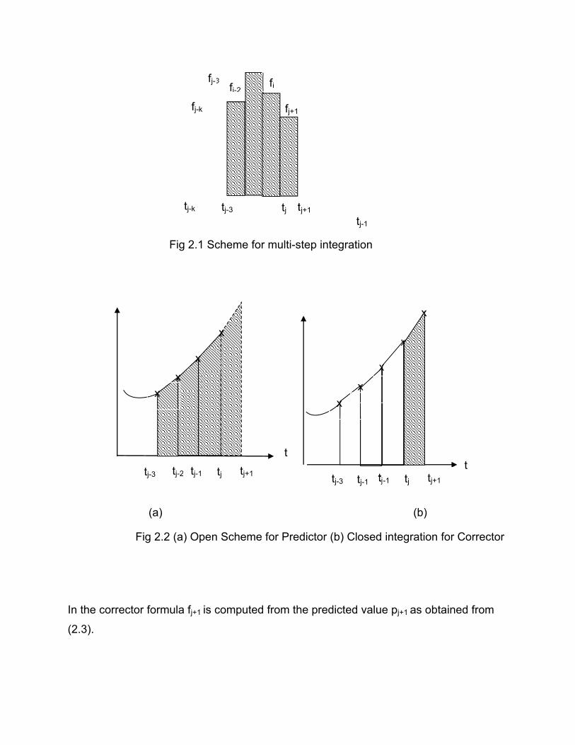
Fig 2.1 Scheme for multi-step integration

(a) (b)

Fig 2.2 (a) Open Scheme for Predictor (b) Closed integration for Corrector

In the corrector formula fj+1 is computed from the predicted value pj+1 as obtained from

(2.3).

tj+1 tj tj-1

tj-3 tj-k

fj-k

fj-3 fj-2

fj+1

t

tj+1 tj tj-2 tj-3

fj

t

x

xj-1

x

tj-1 tj+1 tj tj-3 tj-1 tj-1

x

x

x

x

x

x

Denoting j j jf f(t ,y ) , the equations (2.3) and (2.4) gives the following predictor corrector

formulae, respectively, for solving IVP (2.1) at equi-spaced discrete points t4,t5,…

j 1 j 1 j 3 j j 1 j 2

4hp y y 2f f 2f

3 (2.5)

j 1 j 1 j 1 j j 1

hy y f 4f f

3

The solution at initial point t0 is given in the initial condition and t1, t2 and t3 are the

starting points where solution is to be computed using some other suitable method such

as Runge Kutta method. This is illustrated in the example 2.1

Example 2.1: Solve IVP y’=y+3t-t2 with y(0)=1; using Milne’s predictor corrector method

take h=0.1

Solution: The following table 2.1 computes Starting values using fourth order Runge

Kutta method.

k t

y k1= f(t,y)

t+ h/2

y+ h/2*k1

k2 y+ h/2*k2

k3 t+h

y+ h*k3

k4

y+h(k1+2k2+2k3+k4)/6

0 0 1 1 0.05 1.05 1.19751.05987

51.2074 0.1 1.1207 1.41074 1.1203415

1 0.1 1.1203 1.41034

0.15 1.190859

0.22271.13147

71.559 0.2 1.2762 1.83624 1.2338409

2 0.2 1.2338 1.79384

0.25 1.323533

0.32181.24993

11.9374 0.3 1.4276 2.23758 1.3763387

3 0.2 1.3763

Table 2.1: Starting values using RK4 in Example 2.1

Using initial value and starting values at t=0, 0.1, 0.2 and 0.3, the predictor formula

predicts the solution at t=0.4 as 1.7199359. It is used in corrector formula to give the

corrected value. The solution is continued at advanced grid points [see table 2.2].

Table 2.2: Example 2.1 using predictor corrector method with h=0.1 The exact solution is possible in this example; however it may not be possible for other

equations. Table 2.3 compares the solution with the exact solution of given equation.

Clearly the accuracy is better in predictor corrector method than the Runge-Kutta

method.

rk4 Milne pc exact

0.1 1.120341 1.120342

0.2 1.233841 1.282806

0.3 1.376339 1.489718

0.4 1.5452 1.6771453 1.743649

0.5 1.7369 1.9208947 2.047443

Table 2.3: Comparison of solution of example 2.1

Table 2.4: Example 2.1 using predictor corrector method with h=0.05

The exercise 2.1 is repeated with h=0.5 in table 2.4.The table 2.5 clearly indicates that

the better accuracy is achieved with h=0.05 [see table 2.5]

Milne Predictor corrector1 f(t,p)

k t y f(t,y) corrector

0 0 1 1

1 0.1 1.1203415 1.410341

starting points

2 0.2 1.2338409 1.793841

3 0.3 1.3763387 2.186339

4 0.4 1.7199359 2.759936 1.67714525 2.717145

5 0.5 2.0317593 3.281759 1.920894708 3.170895

Milne Predictor corrector1 f(t,p)

k t y f(t,y)

0 0 1 1

1 0.05 1.055042 1.202542 starting point1

2 0.1 1.120342 1.410342 starting point2

3 0.15 1.196169 1.623669 starting point3

4 0.2 1.282805 1.842805 1.282805 1.842805

5 0.25 1.380551 2.068051 1.380551 2.068051

rk4 Milne pc exact

Table 2.5: improved accuracy with h=0.05

Predictor Corrector methods are preferred over Runge-Kutta as it requires only two

functional evaluations per integration step while the corresponding fourth order Runge-

Kutta requires four evaluations. The starting points are the weakness of predictor-

corrector methods. In Runge kutta methods the step size can be changed easily.

0.05 1.055042 1.055042

0.1 1.120342 1.120342

0.15 1.196169 1.196168

0.2 1.282805 1.282806

0.25 1.380551 1.380551

Module 2

Lecture 2

Multi Step Methods

Predictor corrector Methods

Contd…

Keywords: iterative methods, stability

A predictor-corrector method refers to the use of the predictor equation with one

subsequent application of the corrector equation and the value so obtained is the final

solution at the grid point. This approach is used in example 2.1.

The predicted and corrected values are compared to obtain an estimate of the

truncation error associated with the integration step. The corrected values are accepted

if this error estimate does not exceed a specified maximum value. Otherwise, the

corrected values are rejected and the interval of integration is reduced starting from the

last accepted point. Likewise, if the error estimate becomes unnecessarily small, the

interval of integration may be increased. The predictor formula is more influential in the

stability properties of the predictor-corrector algorithm.

In another more commonly used approach, a predictor formula is used to get a first

estimate of the solution at next grid point and then the corrector formula is applied

iteratively until convergence is obtained. This is an iterative approach and corrector

formula is used iteratively. The number of derivative evaluations required is one greater

than the number of iterations of the corrector and it is clear that this number may in fact

exceed the number required by a Runge-Kutta algorithm. In this case, the stability

properties of the algorithm are completely determined by the corrector equation alone

and the predictor equation only influences the number of iterations required. The step

size is chosen sufficiently small to converge to the solution in one or two iterations. The

step size can be estimated from the error term in (2.4).

Example 2.2: Apply iterative method to solve IVP y’=y+3t-t2 with y(0)=1 with h=0.1

Solution: With h=0.1 the computations are arranged in the table 2.6

Note that the corrector formula converges fast but is not converging to the solution of

the equation. It converges to the fixed point of difference scheme given by the corrector

formula. If h=0.05 then the solution converges to the exact solution in just two iterations.

h k t y f(t,y)

Milne Predictor corrector for t=0.4 with h=0.1

0.1 0 0 1 1

0.1 1 0.1 1.120341 1.410341 starting point1

0.1 2 0.2 1.233841 1.793841 starting point2

0.1 3 0.3 1.376339 2.186339 starting point3

0.1 4 0.4 1.719936 2.759936 predictor

0.1 5 0.4 1.677145 2.717145 corrector1

0.1 6 0.4 1.675719 2.715719 corrector2

0.1 7 0.4 1.675671 2.715671 corrector3

0.1 8 0.4 1.67567 2.71567 corrector4

0.1 9 0.4 1.67567 2.71567 corrector5

Milne Predictor corrector at t=0.5 with h=0.1

0.1 1 0.1 1.120341 1.410341

0.1 2 0.2 1.233841 1.793841 Starting values

0.1 3 0.3 1.376339 2.186339

0.1 4 0.4 1.67567 2.71567

0.1 5 0.5 1.840277 3.090277 predictor

0.1 6 0.5 1.914315 3.164315 corrector1

0.1 7 0.5 1.916783 3.166783 corrector2

0.1 8 0.5 1.916865 3.166865 corrector3

0.1 9 0.5 1.916868 3.166868 corrector4

Table 2.6a iterative Milnes predictor corrector method example 2.2 with h=0.1

Several applications of corrector formula is needed to obtain the desired accuracy.

Decreasing the value of h will reduce the number of applications of corrector formula.

This is evident from the next table 2,6b.

Milne Predictor corrector at t=0.2 for h=0.05 h k t y f(t,y)

0.05 0 0 1 1 0.05 1 0.05 1.055042 1.202542 Starting values

0.05 2 0.1 1.120342 1.4103420.05 3 0.15 1.196169 1.6236690.05 4 0.2 1.282805 1.842805 predictor 0.05 5 0.2 1.282805 1.842805 corrector1 0.05 6 0.2 1.282805 1.842805 corrector2

Table 2.6b iterative Milnes predictor corrector method example 2.2 with h=0.05

A modified method, or modified predictor-corrector method, refers to the use of the

predictor equation and one subsequent application of the corrector equation with

incorporation of the error estimates as discussed below

Error estimates

Local Truncation Error in predictor and corrector formulae are given as

5 (4)j 1 j 1 j 3 j 1

28y(t ) p h f ( ); in(t ,t )

90

5 (4)j 1 j 1 j 1 j 1

1y(t ) y h f ( ); in(t ,t )

90

It is assumed that the derivative is constant over the interval [tj-3, tj+1]. Then simplification

yields the error estimates based on predicted and corrected values.

j 1 j 1 j 1 j 1

28y(t ) p [y p ]

29 (2.6)

Further, assume that the difference between predicted and corrected values at each

step changes slowly. Accordingly, pj and yj can be substituted for pj+1 and yj+1 in (2.6)

gives a modifier qj+1 as

j 1 j 1 j j

28q p [y p ]

29

This modified value is used in functional evaluation fj+1 to be substituted in corrector

formula. This scheme is known as Modified Predictor corrector formula and is given as

j 1 j 1 j j j 1 j 2

4hp y y 2f f 2f

3

j 1 j 1 j j j 1 j 1 j 1

28q p [y p ]; f f(t ,q )

29 (2.7)

j 1 j j 1 j j 1

hy y f 4f f

3

Another problem associated with Milne’s predictor corrector method is the instability

problem in certain cases. This means that error does not tend to zero as h tends to

zero. This is illustrated analytically for a simple IVP

Y’=Ay, y(0)=y0

Its solution at t=tn is yn=y0 exp(tn-t0). Substituting y’=Ay in the corrector formula gives the

difference equation

j 1 j 1 j 1 j j 1

hy y Ay 4Ay Ay

3

Or j 1 j j 1

hA 4hA hA(1 )y y (1 )y 0

3 3 3 (2.8)

Let Z1 and Z2 be the roots of quadratic equation

2hA 4hA hA(1 )Z Z (1 ) 0

3 3 3

The solution of above difference equation (2.8) can be written as

2j j

j 1 1 2 2 1,2

2r 3r 1 hAy C Z C Z ;with Z ,r

1 r 3

For stability the behavior of solution is to be explored as h tends to zero, consider

22 2

1

22 2

2

2r 3r 1Z 1 3r O(r ) 1 Ah O(h )

1 r

2r 3r 1 AhZ 1 r O(r ) (1 ) O(h )

1 r 3

Also, 2 2exp(hA) 1 hA O(h ),exp( hA / 3) 1 hA / 3 O(h ),

Hence the solution of the given IVP by predictor corrector method is represented as

j 1 j 0 2 j 0y C exp A(t t ) C exp A(t t ) / 3

When A>0, the second term will die out but the first grows exponentially as j increases

irrespective of h. However, first term will die out and second will grow exponentially

when A<0. This establishes the instability of the solution.

Module 2

Lecture 3

Multi Step Methods

Adams Bashforth method

Keywords: interpolating polynomial, open integration

A general k step method for solving IVP is given as

j 1 k 1 j k 2 j 1 0 j 1 m

k j 1 j 1 k 1 j j 0 j 1 m j 1 m

y a y a y ... a y

h[b f(t ,y ) b f(t ,y ) ... b f(t ,y )

(2.9)

When bk=0, the method is explicit and yj+1 is explicitly determined from the initial value y0

and starting values yi; i=1,2, …, k-1. When bk is nonzero, the method is implicit.

The Milne’s predictor corrector formulae are the special cases of (2.9):

Predictor formula 1 2 3 4 0 1 2 3 4: k=4,a =a =a =0,a =1,b =0, b =8/3, b =-4/3, b =8/3, b =0

Corrector formula 1 2 4 3 0 1 2 3 4: k=4,a =a =a =0,a =1,b =0, b =0, b =1, b =4, b =1 .

Another category of multistep methods, known as Adams methods, are obtained from

j 1 j 1

j j k

t t rj

j 1 j j jj 0t t


Here the integration is carried out only on the last panel, while many function and

derivative values at equi-spaced points are considered for the interpolating polynomial.

Both open and closed integration are considered giving two types of formulas. The

integration scheme is shown in the fig. 2.3

Fig. 2.3 Schematic diagram for open and closed Adams integration

formulas

t

x

x

x

tj+1 tj tj-3 tj-1 tj-1 t

x

x

tj+1 tj tj-3 tj-1 tj-1

x x x

x

The open integration of Adams formula gives Adams Bashforth formula while

closed integration gives Adams Moulton formula. Different degrees of interpolating

polynomials depending upon the number r of interpolating points give rise to formulae of

different order. Although these formulae can be derived in many different ways, here

backward application of Taylor series expansion is used for the derivation of second

order Adams Bashforth open formula.

Second Order Adams Bashforth open formula

For second order formula, consider degree of polynomial r=2 and points tj, tj-1and tj-2

are used in the following

j 1 j 1

j j k

t t 2j

j 1 j j jj 0t t


Expanding left hand side in Taylor series as

2j 1 j j j jy y h[f f h / 2 f h / 6 ...]

(2.10)

Also, j j 1 j 2

j

f f ff h O(h )

h 2

Substitution and simplification yields second order Adams formula

3j 1 j j j 1 j

3 1 5y y h( f f ) h f ( )

2 2 12 (2.11)

A fourth order Adams Bashforth formula can be derived on similar lines and it is written

as

5 ivj 1 j j j 1 j 2 j 3

55 59 37 9 251y y h( f f f f ) h f ( )

24 24 24 24 720 (2.12)

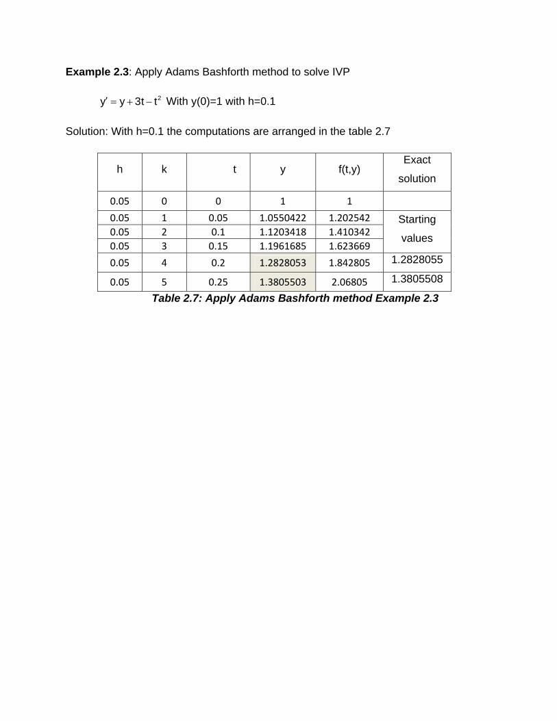
Example 2.3: Apply Adams Bashforth method to solve IVP

2y y 3t t With y(0)=1 with h=0.1

Solution: With h=0.1 the computations are arranged in the table 2.7

h k t y f(t,y) Exact

solution

0.05 0 0 1 1

0.05 1 0.05 1.0550422 1.202542 Starting

values 0.05 2 0.1 1.1203418 1.410342

0.05 3 0.15 1.1961685 1.623669

0.05 4 0.2 1.2828053 1.842805 1.2828055

0.05 5 0.25 1.3805503 2.06805 1.3805508

Table 2.7: Apply Adams Bashforth method Example 2.3

Module 2

Lecture 4

Multi Step Methods

Adams Moulton method

Keywords: closed integration, local truncation error

Second Order Adams Moulton formula

Backward Taylor series is used for integrand in the closed integration formula:

j 1 j 1

j j k

t t 2j

j 1 j j jj 0t t


2j j 1 j 1 j 1 j 1y y h[f f h / 2 f h / 6 ...]

(2.13)

2j 1 j j 1 j 1 j 1y y h[f f h / 2 f h / 6 ...]

j 1 j j 1 2j 1

f f ff h O(h )

h 2

Substitution and simplification yields second order Adams Moulton formula

3j 1 j j 1 j j 1

1 1 1y y h( f f ) h f ( )

2 2 12 (2.14)

Fourth order Adams Moulton formula can be obtained on similar lines:

5 ivj 1 j j 1 j j 1 j 2

9 19 5 1 19y y h( f f f f ) h f ( )

24 24 24 24 720 (2.15)

A predictor corrector method is based on Adams integration formulas make use of

Adams Bashforth formula (2.12) as predictor while Adams Moulton formula (2.15) as

corrector. Milne’s method is considered to be better due to smaller error terms.

However, Adams method is preferred due to instability of corrector formula in Milne’s

method in some cases.

The predictor formula

5 ivj 1 j j j 1 j 2 j 3

55 59 37 9 251y y h( f f f f ) h f ( )

24 24 24 24 720

The Corrector formula

5 ivj 1 j j 1 j j 1 j 2

9 19 5 1 19y y h( f f f f ) h f ( )

24 24 24 24 720

Example 2.4 Solve IVP of example 2.3 by Adams predictor corrector Method

h k t y f(t,y)

Solution At t=0.20

0.05 0 0 1 1

0.05 1 0.05 1.0550422 1.202542Starting

values 0.05 2 0.1 1.1203418 1.410342

0.05 3 0.15 1.1961685 1.623669

0.05 4 0.2 1.2828053 1.842805 predictor

0.05 5 0.2 1.2828055 1.842806 corrector

0.05 6 0.2 1.2828056 1.842806 corrector

Solution At t=0.25

0.05 1 0.05 1.0550422 1.2025420.05 2 0.1 1.1203418 1.410342

Starting values

0.05 3 0.15 1.1961685 1.6236690.05 4 0.2 1.2828056 1.8428060.05 5 0.25 1.3805506 2.068051 predictor 0.05 6 0.25 1.3805509 2.068051 corrector 0.05 7 0.25 1.3805509 2.068051 corrector

Table 2.8 Solution of IVP of Example 2.3 by Adams predictor corrector Method

Both the predictor and corrector formula have Local Truncation errors of order O(h5):

( )

( )

( ) ( )

( ) ( )

5 5k 1 k 1 1

5 5k 1 k 1 2

251y t p y h

72019

y t y y h720

If fifth derivative is nearly constant and h is small then the error estimate can be

obtained by eliminating the derivative and simplifying as

( ) ( )k 1 k 1 k 1 k 1

19y t y y t p

270

Exercise 2

2.1 Consider the IVP

,ty e y y(0)=1

Compute solution at times t=0.05, 0.1 and 0.15 using RK4 by taking h=0.05. Use

these values to compute solution at t=0.2 0.25 and 0.3 using Milne-Simpson

method. Compare solution with the exact solution ( ) ty t 1 e

2.2 Consider the IVP

,2y y t y(0)=1

Compute solution at times t=0.2, 0.4 and 0.6 using RK4 by taking h=0.2. Apply

Adams Bashforth method to compute solution at t=0.8 and 1.00

2.3 Solve IVP of exercise 2.2 by fourth order Adams predictor corrector Method.


Module 3

Systems of equations and higher order equations

keywords: system of differential equations, Euler method, Runge-Kutta methods

Systems of Differential Equations

The mathematical models of many real life dynamical problems give rise to system of first order

differential equations. For example, dynamics of interacting species, chemical or biological, at

molecular, cellular or population level is modeled as a system of n first order differential

equations. The number n depends upon the species involved in the interaction. The study of

combustion dynamics can give a large system with n in hundreds or even in thousands. The

system of differential equations generally involved wide variety of possible behaviors as

compared to single differential equation. As such more advanced mathematics is required for

their analysis. However when it comes to numerical techniques for solving them, there is not

much difference between the system of differential equations and single differential equations.

The most general form of a system of m differential equations can be written as

i i 1 2 3 m i 0iy (t) f t,y ,y ,y ,...y t ;y (0) y ;0 a t b (3.1)

In (3.1) t is independent variable and m dependent variables are 1 2 3 my ,y ,y ,...y . Introducing

column vector Y as T1 2 3 m(y ,y ,y ,...y ) , F as T

1 2 3 m(f , f , f ,...f ) and Y0 as T01 02 03 0m(y ,y ,y ,...y ) , the

system (3.1) in matrix form is written as

0Y (t) F(t,Y);Y(0) Y ;0 t b (3.2)

The form (3.2) is similar to the IVP (1.2) with scalars being replaced by vectors.

Let the interval (a,b) is divided into N subintervals of width h=(b-a)/N such that the grid

points are tj=a+jh and tj+1=tj+h. Let yi,j ; i=1,2,…m and j=1,2,…N denote the

approximation of ith dependent variable yi (tj) at t=tj=t0+jh.

The Eulers method for the system of equations be written as

i,j 1 i,j i j 1,j 2,j m,jy y hf (t ,y ,y ,...,y );i 1,2,...,m and j 0,1,2,...,N (3.3)

Fourth Order Runge Kutta method for system of equations

1,i i j 1,j 2,j 3,j m,j

2,i i j 1,j 1,1 2,j 1,2 3,j 1,3 m,j 1,m

3,i i j 1,j 2,1 2,j 2,2 3,j 2,3 m,j 2,m

4,i i j 1

K f t ,y ,y ,y ,...,y , ;i 1,2,...,m

h h h h hK f t ,y K ,y K ,y K ,...,y K

2 2 2 2 2

h h h h hK f t ,y K ,y K ,y K ,...,y K

2 2 2 2 2

K f t h,y

,j 3,1 2,j 3,2 3,j 3,3 m,j 3,m

1,i 2,i 3,i 4,i

hK ,y hK ,y hK ,...,y hK

hyi, j 1 yi, j K 2K 2K K

6

(3.4)

Example 3.1 Solve the system of differential equations with given initial conditions

using Eulers method in the interval (0,1) taking h=0.02

x =x+2y x(0)=6

y =3x+2y y(0)=4

Solution: The Euler method given in (3.3) is used for solving given system of two

equations (m=2):

1

2

f (x,y)=x+2y x(0)=6

f (x,y)=3x+2y y(0)=4

The computations are shown in the table 3.1.

j h t xj yj f1 f2

0 0.02 0 6 4 14 26

1 0.02 0.02 6.28 4.52 15.32 27.88

2 0.02 0.04 6.5864 5.0776 16.7416 29.9144

3 0.02 0.06 6.921232 5.675888 18.273008 32.115472

4 0.02 0.08 7.28669216 6.31819744 19.923087 34.49647136

5 0.02 0.1 7.685153901 7.00812687 21.7014076 37.07171544

6 0.02 0.12 8.119182054 7.74956118 23.6183044 39.85666851

7 0.02 0.14 8.591548142 8.54669455 25.6849372 42.86803352

8 0.02 0.16 9.105246886 9.40405522 27.9133573 46.12385109

9 0.02 0.18 9.663514033 10.3265322 30.3165785 49.64360657

10 0.02 0.2 10.2698456 11.3194044 32.9086543 53.44834555

11 0.02 0.22 10.92801869 12.3883713 35.7047613 57.56079863

Table 3.1 Solution of Example 3.1

Refer to euler-system of equations.xlsx

Example 3.2 Solve the following system of differential equations with given initial

conditions using fourth order Runge Kutta method in the interval (0, 2) taking h=0. 5

x =x-xy x(0)=4

y =-y+xy y(0)=1

Solution: Consider the system with h=0.5, m=2

1

2

f (x,y)=x-xy x(0)=4

f (x,y)=-y+xy y(0)=1

The Runge-Kutta formulae given in (3.4) are used to compute solution. The

computations are shown in the table 3.2 [Ref. system_of_equations.xls]

t x y k11=f1(x,y) k12=f2(x,y) 0 4 1 0 3

t+h/2 x+h*k11/2 y+h*k12/2 k21=f1(x,y) k22=f2(x,y)

0.25 4 1.75 -3 5.25

t+h/2 x+h*k21/2 y+h*k22/2 k31=f1(x,y) k32=f2(x,y)

0.25 3.25 2.3125 -4.265625 5.203125

t+h x+h*k31 y+h*k32 k41=f1(x,y) k42=f2(x,y)

0.5 1.8671875 3.6015625 -4.85760498 3.12322998

phi1 phi2

-1.61573792 2.25245667

t1 x+phi1 y+phi2

0.5 2.384262085 3.252456665

t1 x y k11=f1(x,y) k12=f2(x,y)

0.5 2.384262085 3.252456665 -5.37044702 4.50225244

t1+h/2 x+h*k11/2 y+h*k12/2 k21=f1(x,y) k22=f2(x,y)

0.75 1.041650329 4.378019776 -3.51871541 0.18234596


0.75 1.504583232 3.298043156 -3.4575972 1.66413728

t1+h x+h*k31 y+h*k32 k41=f1(x,y) k42=f2(x,y)

1 0.655463485 4.084525303 -2.02179371 -1.40726811

phi1 phi2

-1.77873883 0.56566257

t2 x+phi1 y+phi2

1 0.605523256 3.818119233

t2 x y k11=f1(x,y) k12=f2(x,y)

1 0.605523256 3.818119233 -1.70643673 -1.50615924


1.25 0.178914073 3.441579422 -0.43683292 -2.82583243


1.25 0.496315026 3.111661125 -1.04804915 -1.56729695


1.5 0.081498682 3.034470757 -0.16580669 -2.78716539

phi1 phi2

-0.40350063 -1.08996528

t3 x+phi1 y+phi2

1.5 0.202022627 2.728153949

t3 x y k11=f1(x,y) k12=f2(x,y)

1.5 0.202022627 2.728153949 -0.3491262 -2.17700512


1.25 0.114741077 2.183902669 -0.13584227 -1.93331933


0.25 0.16806206 2.244824118 -0.20920771 -1.86755435


2 0.097418774 1.794376773 -0.07738721 -1.61957079

2 phi1 x+phi1 phi2 y+phi2

-0.09305111 0.108971514 -0.94986027 1.778293677 Table 3.2: Solution of the system of equations in Example 3.2

Accordingly, the first part of the table gives x(0.5)=2.384262085, y(0.5)=

3.252456665.The solution at t=1.0,1.5 and 2.0 are computed in the subsequent parts of

the table

Module 3

Lecture 2

Numerical Solution of Higher Order Ordinary Differential Equations

keywords: system of differential equations, Euler method, Runge-Kutta methods

Solution of Higher Order Ordinary Differential Equations

The general form of an nth order differential equation is

(n) (n 1)F(y ,y ,...,y ,y ,y,t) 0 (3.5)

It is convenient to convert higher order differential equation to a system of first order differential

equations. This is illustrated for the following second order differential equation n=2:

F(y ,y ,y,t) 0 (3.6)

The initial conditions associated with ( 3.6)

0 1y(0)=y and y (0)=y

Substituting z=y’ in (3.6) givesF(z ,z,y,t) 0 .

Accordingly, the second order equation (3.6) reduces to a system of two coupled first order

equations in two unknowns y and z:

z y

F(z ,z,y,t) 0

Or y z

z f(z,y,t)

(3.7)

The associated initial conditions get transformed to

0 1y(0)=y and z(0)=y (3.8)

Let TY y, z , the system can be written in the matrix form as

TY G(y,z,t);G z,f(y,z,t) With initial condition T0 1Y(0) (y ,y ) (3.9)

The second order differential equation is reduced to a system of two first order

differential equation in two unknowns y and y’. Similarly nth order differential equation

can be reduced to a system of n first order differential equation in n unknowns y ,

y’,…,y(n-1) .Once the higher order differential equation is converted into system of first

order differential equations, then one of the methods already discussed can be applied.

Example 3.3 Solve the following initial value problem using fourth order Runge Kutta

method in the interval (1, 2) taking h=0.2

( ) , ( ) ,2

22

x 1

d x dx dx2x 1 0 x 1 1 0

dt dt dt

Solution: Writing dx

ydt

, the given differential equation becomes

2dy 1 y

dt 2x

Therefore, the equivalent system of equations is

( , ), ( , )2

1 2

dx dy 1 yy f x y f x y

dt dt 2x

The system is subjected to initial conditions x(1)=1, y(1)=0.The following table shows

the detailed computational steps for solution at t=1.2 when h=1.2

j h t x y k11=f1(x,y) k12=f2(x,y)

0 0.2 1 1 0 0 -0.5

t+h/2 x+h*k11/2 y+h*k12(x,y)/2 k21=f1(x,y) k22=f2(x,y)

1.1 1 -0.05 -0.05 -0.50125

t+h/2 x+h*k21/2 y+h*k22(x,y)/2 k31=f1(x,y) k32=f2(x,y)

1.1 0.995 -0.05013 -0.05013 -0.50378

t+h x+h*k31 y+h*k32(x,y) k41=f1(x,y) k42=f2(x,y)

1.2 0.989975 -0.10076 -0.10076 -0.51019

1.2 phi1 x+phi1 phi2 y+phi2

-0.01003 0.989966 -0.10067 -0.10067

Table 3.3: Solution of the system of equations in Example 3.3 at t=1.2

Solution at other time steps are obtained similarly and given in the next table. Details of

steps can be seen in the excel sheet second-order ODE-RK4ex3.3 .xls.

x(1) x(1.2) x(1.4) x(1.6) x(1.8) x(2)

1 0.989966 0.959451 0.907106 0.830285 0.724106

Table 3.4: Complete Solution of the system of equations in Example 3.3

Module 3

Lecture 3

Stiff Differential Equations

keywords: Euler method, explicit method, implicit method, stiff equations, stability

Stiff Differential Equations

It is observed that the approximate solution of ordinary differential equations involve

truncation error which depends upon the higher derivatives of the solution. When this

higher derivative is bounded then the method gives predictable error bound. In some

cases the solutions as well as its derivative(s) grow with number of steps and the

relative error can still be under control. However, there are IVP for which the error grows

so large that the solution is not acceptable. Such equations are termed as stiff

equations. These are very common in physical and biological systems. One typical

example is mass spring system with a large spring constant (stiffness).

The stiff equations are characterized by those differential equations having a term of the

form exp(-ct) in the exact solution with large c. Typically, this led to fast decaying

transient solution. But the increasing truncation error (involving its nth derivative) of the

form cn exp (-ct) will destabilize the approximate solution. In such cases the step size h

should be drastically decreased to maintain stability. The following stiff differential

equation involves large negative exponent in the solution

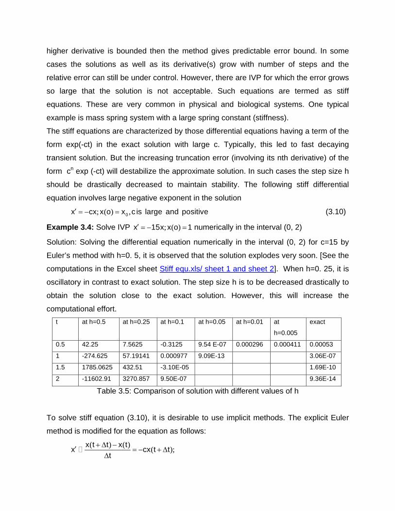
; ( ) ,0x cx x o x c is large and positive (3.10)

Example 3.4: Solve IVP ; ( )x 15x x o 1 numerically in the interval (0, 2)

Solution: Solving the differential equation numerically in the interval (0, 2) for c=15 by

Euler’s method with h=0. 5, it is observed that the solution explodes very soon. [See the

computations in the Excel sheet Stiff equ.xls/ sheet 1 and sheet 2]. When h=0. 25, it is

oscillatory in contrast to exact solution. The step size h is to be decreased drastically to

obtain the solution close to the exact solution. However, this will increase the

computational effort.

t at h=0.5 at h=0.25 at h=0.1 at h=0.05 at h=0.01 at

h=0.005

exact

0.5 42.25 7.5625 -0.3125 9.54 E-07 0.000296 0.000411 0.00053

1 -274.625 57.19141 0.000977 9.09E-13 3.06E-07

1.5 1785.0625 432.51 -3.10E-05 1.69E-10

2 -11602.91 3270.857 9.50E-07 9.36E-14

Table 3.5: Comparison of solution with different values of h

To solve stiff equation (3.10), it is desirable to use implicit methods. The explicit Euler

method is modified for the equation as follows:

( ) ( )

( );x t t x t

x cx t tt

Or ( )

( )x t

x t t1 c t

(3.11)

The application of this Euler implicit scheme for the equation (3.10) will not misbehave.

[See the computations in the Excel sheet Stiff equ.xls/ sheet 3]

In case of IVP ( , ); ( ) 0x f x t x o x

The implicit Euler Scheme is written as

( , )k 1 k k 1 k 1x x hf x t (3.12)

Another implicit scheme which can be used to solve stiff equations is Trapezoidal

scheme or two stage adams Moulton scheme

[ ( , ) ( , )] /k 1 k k k k 1 k 1x x h f x t f x t 2 (3.13)

The stiff differential equations generally results from the phenomenon that involves

widely differing time scales. Consider the differential equation

x 100x

Its most general solution is

( ) 10t 10tx t Ae Be

There are two different time scale in the solution. In another example

; ( )tx 1000x e x o 1

Its exact solution also involves two time scales 1 versus 1/1000

( ) ( ) /1000t tx t e e 999

In general the presence of vastly different evolutionary time scale gives stiff dynamic

differential equations. In such cases, care should be taken in solving them.

Example 3.5: Using Euler implicit Scheme Solve IVP over interval (0, 3.0)

; ( )tx 1000x e x o 1 . Take h=0.05

Solution: Applying Scheme (3.12) to the given equation gives

k k 1k 1

x hexp( t )x

1 1000h

The numerical details are worked out in Excel file Stiff equ.xls/ sheet 4

euler method

h tk xk f(xk,tk) xk+1 exact

0.05 0 1 -1001 -49.05 0.05 -0.000952182

0.05 0.05 -49.05 49049.0488 2403.40244 0.1 -0.000905743

0.05 0.1 2403.40244 -2403403.3 -117766.765 0.15 -0.00086157

0.05 0.15 -117766.765 117766764 5770571.43 0.2 -0.00081955

0.05 0.2 5770571.43 -5.771E+09 -282758000 0.25 -0.00077958

0.05 0.25 -282758000 2.8276E+11 1.3855E+10 0.3 -0.00074156

0.05 0.3 1.3855E+10 -1.386E+13 -6.789E+11 0.35 -0.000705393

Table 3.6 a Euler I Method for stiff equation

Euler Implict method

h tk xk tk+1 hexp(-tk+1) xk+1 exact

0.05 0 1 0.05 0.951229 0.0186753 -0.000952182

0.05 0.05 0.018675 0.1 0.904837 -0.0005209 -0.000905743

0.05 0.1 -0.00052 0.15 0.860708 -0.000854 -0.00086157

0.05 0.15 -0.00085 0.2 0.818731 -0.0008194 -0.00081955

0.05 0.2 -0.00082 0.25 0.778801 -0.0007796 -0.00077958

0.05 0.25 -0.00078 0.3 0.740818 -0.0007416 -0.00074156

0.05 0.3 -0.00074 0.35 0.704688 -0.0007054 -0.000705393

Table 3.6 b Euler Implicit Method for stiff equation

Exercise 3

3.1 Solve the following system of equations using Runge Kutta method of

order 4 in the interval 0< t 1.0 :

(a) ; ( )

; ( )

x xy t x 0 1

y ty x y 0 1

; taking h=0.1

(b) ; ( )

; ( )

x x 4y x 0 2

y y x y 0 3

; taking h=0.0.5

(c) ; ( )

; ( ) .

2 2x y x x 0 2

y 2xy y 0 0 1

; taking h=0.0.5

(d) ( ) ; ( )

( ) ; ( )

2 2t

2 2t

x 3x 2y 2t 1 e x 0 1

y 4x y t 2t 4 e y 0 1

; taking h=0.1

3.2 Solve the following higher order differential equations using Runge Kutta

method of order 4

(a) ln , ; ( ) , ( )2 3t x 2tx 2x t t 1 t 2 x 1 1 x 1 0

3.3 Using trapezoidal Scheme Solve IVP over interval (0, 3.0)

; ( )tx 1000x e x o 1 . Take h=0.05

Repeat the exercise for h = 0.001

Module 4 Linear Boundary value problems


1 Finite Difference Methods: Dirichlet type boundary condition

1

2 Finite Difference Methods: Mixed boundary condition 1

3 Shooting Method 1

4 Shooting Method contd… 1

Module 4 Lecture 1

Finite Difference Methods: Dirichlet type boundary condition

keywords: Dirichlet type boundary conditions, discretize, finite differences

Linear Boundary Value Problems

An initial value problem consists of a differential equation and associated initial

conditions for finding the unique solution of the problem. All the initial conditions are

specified at one specified point called as initial point. Typical initial conditions for nth

order differential equation involve specification of y, y’,…,y(n-1) at some initial point, say

at t=0. For a boundary value problem boundary conditions are associated with the

differential equation. The boundary conditions are specified at different points of the

domain of independent variable t known as boundary points. For example, consider a

second order ordinary differential equation

1 1 1

2 2 2

y f(y ,y,x);a x b

(x)y(x) (x)y (x) at x a

(x)y(x) (x)y (x) at x b

(4.1)

The Boundary value is called two-point linear boundary value problem when the

arbitrary function f is given as a linear combination of dependent variable and its

derivative as

f(y ,y,x) c(x)y (x) d(x)y(x) e(x) (4.2)

The boundary conditions are specified at the boundary points x=a and x=b as linear

combination of y and its derivative y’. This is Robin mixed boundary conditions. In

particular when i i0, 0;i 1,2 then the boundary conditions are known as Dirichlet

boundary conditions. The conditions are Neumann’s boundary conditions when

i i0, 0;i 1,2

Finite difference method for two point linear Boundary Value problem with Dirichlet type

conditions

1 2

y c(x)y (x) d(x)y(x) e(x);a x b

y(a) ; y(b)

(4.3)

To apply finite difference method first discretize the domain a x b into N-1

computational grid points ix ;i 1,2...N 1 and two boundary points 0x and Nx as

0 1 2 N 1 Na x x x ... x x b

The grid points are equi-spaced and computed as

i 0b a

x x ih;hN

The step size h is a critical parameter for stability and convergence of the numerical

scheme. The differential equation is now written at each internal grid point

ix ;i 1,2...N 1 . For this, the derivatives are replaced by corresponding finite differences:

2i 1 i i 1i 2

2i 1 i 1i

y 2y yy x o(h )

hy y

y x o(h )2h

that is

i 1 i i 1 i 1 i 1i i i i2

y 2y y y yc(x ) d(x )y e(x )

2hh

or 2 2i i 1 i i i i 1 i

h h( 1 c )y (2 h d )y ( 1 c )y h e ;i 1,2,N 1

2 2 (4.4)

The unknown yi’s are on the left side and known quantities are on right side of

the equation for i=2,3,…N-2. Using boundary conditions for i=1and i=N-1 give

2 21 1 1 2 1 1 1

h h(2 h d )y ( 1 c )y h e (1 c )

2 2 (4.6a)

2 2N 1 N 2 N 1 N 1 N 1 N 1 2

h h( 1 c )y (2 h d )y [h e (1 c ) ]

2 2 (4.6b)

This reduces the system of differential equations to linear system of N-1 algebraic

equations which can be written in the matrix form as AX=B where

1 1

2 2 2

N 2 N 2 N 2

N 1 N 1 (N 1)X(N 1)

u

u

. ... .

. ...

u

2i i

i i

i i

2 h d

h1 c

2h

u 1 c2

1

2

N 2

N 1

x

x

X .

x

x

21 1

22

2N 2

2N 1 2

hh e (1 )

2

h e

B ...

h e

hh e (1 )

2

(4.7)

The system of equations must admit unique solution for which the sufficient condition is

the diagonal dominance of the matrix A. Suppose d(x) has positive values in the domain

and c(x) is continuous. Let L be upper bound of the function c(x) over the domain then

the step size h smaller than 2/L guarantees the uniqueness of the solution.

Example 4.1: Solve the boundary value problem using N=4

y 12y 16;y(0) y(2) 5

Solution: It is observed that c(x)=0, d(x)=12>0, e(x)=-16. for N=4, the Bvp will

reduce to system of three algebraic equations with step size h=2/4=0.5 The equivalent

system given below:

1 2

1 2 3

2 3

5y y 1

y 5y y 4

y 5y 1

The system of algebraic equations corresponding to the BVP has unique solution

irrespective of step size h. The solution of the system is

1 2 31 18 1

y ,y ,y23 23 23

Example 4.1: Solve the boundary value problem using N=4

3xy (2x 1)y (x 1)y; y(1) 2e,y(3) 10e

Solution: For the given boundary value problem a=1, b=3, N=4 h=0.5

2x 1 x 1c(x) ,d(x) ,e(x) 0

x x

It may be noted that d(x) is positive and c(x) is a decreasing function in (1, 3).

Therefore, L=C(1)=3. Accordingly, the condition for unique solution ( h<2/L) is satisfied

for h=0.5

The grid points are 0 1 2 3 4x 1.0,x 1.5,x 2.0,x 2.5,x 3.0

The coefficients of the matrix are computed from the expressions given below

2i i ii i i

i i i

x 1 2x 1 2x 1h hd 2 h , 1 ( ) ,u 1 ( ) ,

x x 2 x 2

Applying finite differences gives the following system of equations:

1 2

1 2 3

2 3

2.41667y -0.33333y =9.060939

-1.625 y +2.375 y -0.375 y =0

-1.6 y +2.35 y =80.34215

The coefficient matrix is diagonally dominant. The system of equations can be solved

using Gauss-Seidel iterative scheme with initial guess as (0,0,0).

For numeric computations refer to NPTEL-II\BVP-I.xls

The final solution is obtained as

1 2 3y =5.125596, y =9.977751, y =40.98151

Documents

Lecture 1