Learning Movement Primitive Attractor Goals and Sequential Skills from

Kinesthetic Demonstrations

Simon Manschitza,b,∗, Jens Koberc, Michael Giengerb, Jan Petersa,d

aInstitute for Intelligent Autonomous Systems,Technische Universitat Darmstadt, 64289 Darmstadt, GermanybHonda Research Institute Europe, 63073 Offenbach, Germany

cDelft Center for Systems and Control, Delft University of Technology, 2628 CD Delft, The NetherlandsdMax Planck Institute for Intelligent Systems, 72076 Tubingen, Germany

Abstract

We present an approach for learning sequential robot skills through kinesthetic teaching. In our work, finding thetransitions between consecutive movement primitives is treated as multiclass classification problem. We show how the goalparameters of linear attractor movement primitives can be learned from manually segmented and labelled demonstrationsand how the observed movement primitive order can help to improve the movement reproduction. The improvement isachieved by restricting the classification result to the currently activated movement primitive and its possible successorsin a graph representation of the sequence, which is also learned from the demonstrations. The approach is validated withthree experiments using a Barrett wam robot.

Keywords: human-robot interaction, kinesthetic teaching, learning from demonstration, programming by demonstration

1. Introduction

Adapting skills to new situations is arguably one ofthe key elements for robots to become more autonomous.Learning from demonstration (lfd) or imitation learningtherefore has received a lot of attention in robotics researchin the past years. The goal of lfd is to learn skills basedon demonstrations of a teacher [1]. While most work in thisdomain concentrates on learning single movement skills,sequencing such learned skills in order to perform moresophisticated tasks is still an open research topic. Thereare two cases where such sequential skills are particularlyuseful. First, there are tasks which are not representablein a non-sequential way at all. As an example, consider arobot standing in front of a door. Without any additionalknowledge, the system does not know whether the robothas to open the door or if the robot just closed it. Thereason is that the same state is perceived for both options.This problem is often referred to as perceptual aliasing [29].Dissolving perceptual aliasing requires either the previousmovement history to be encoded in the perceived state or apolicy which activates movements based on the history ofmovements. Such a policy is what we call a sequential skill.Second, even though a task may be representable using asingle movement, it may be beneficial to decompose it into

∗Corresponding authorEmail addresses: manschitz@ias.tu-darmstadt.de

(Simon Manschitz), j.kober@tudelft.nl (Jens Kober),michael.gienger@honda-ri.de (Michael Gienger),mail@jan-peters.net (Jan Peters)

Kinesthetic Demonstration Reproduction & Generalization

Figure 1: The system is supposed to learn how to unscrewa light bulb from kinesthetic demonstrations. We evaluateour approach on this example using a real seven degrees offreedom (dof) Barrett wam robot with a four dof hand.

smaller (sub-)tasks first. Such a decomposition bounds thecomplexity of each (sub-)task and the resulting movementsare often more intuitive and easier to learn.

We aim at learning sequential skills where the currentlyactivated movement cannot be solely determined from theperceived state, but may also depend on the history ofmovements. The goal is to learn when to activate eachmovement, based on kinesthetic demonstrations. Kines-thetic teaching is a widely used teaching method in robotics.Here, a teacher guides a robot through movements by phys-ically moving the robot’s arm, similar to parents teachingtasks to their children. (see Figure 1).

Preprint submitted to Robotics and Autonomous Systems October 5, 2015

1.1. Related Work

Single elementary movements are often referred to asmovement primitives (mps) in literature [10, 26]. Thetraditional way of sequencing mps was inspired by the sub-sumption architecture [3], where the behavior of a system isrepresented by a hierarchy of sub-behaviors. A sequentialskill is usually composed by a two-level hierarchy, wherebythe lower-level mps are activated by an upper-level sequenc-ing layer. The sequencing layer is usually modeled as graphstructure, finite state machine (fsm) or Petri net and theactivation of a mp is interpreted as discrete event in acontinuous system [25, 24, 6]. An alternative view is treat-ing the overall system as continuous entity. For example,Luksch et al. [14] model a sequence with a recurrent neuralnetwork. In that architecture, mps can be concurrentlyactive and inhibit each other. Therefore the sequence isdefined implicitly. Although this structure leads to verysmooth movements, the model is hard to learn and has tobe defined mostly by hand.

Most concepts for sequencing mps concentrate eitheron segmenting demonstrations into a set of mps and/oron learning the individual mp parameters [21, 7, 27, 18].Reproducing a sequence of learned mps then serves as proofof concept for the segmentation. The actual sequence is notso important here, therefore the mps are chosen randomlyor are the same as in the demonstrations [13, 15]. Thetransition behavior between mps is also either determin-istic (e.g., the succeeding movement depends only on theprevious movement) or not learned at all [11]. For trigger-ing transitions, often subgoals or sequential constraints of atask are used [9, 19]. Sequential constraints (e.g., subtask Ahas to be executed before subtask B) can also be used toextract symbolic descriptions of tasks [22, 28, 12]. Sucha description implicitly determines the mp sequence andis often intuitive. Indeed, symbolic approaches can per-form sufficiently well for predetermined settings. However,they lack generality as they rely on predefined assumptionsabout the tasks. If these assumptions do not fully apply,they are likely to bias the system towards suboptimal deci-sions. Therefore probabilistic methods have become morepopular, as they allow for a better generalization.

In [23], a nearest neighbor classifier is used to decidewhich mp to activate when the current movement has fin-ished. Butterfield et al. [4] use a hierarchical Dirichletprocess hidden Markov model as classification method fordetermining the next mp based on the sensor informationand current mp. Niekum et al. [20] segment a demonstra-tion with a beta process auto-regressive hidden Markovmodel in a set of mps and build a fsm on the sequentiallevel. The transition behavior is learned with k-nearestneighbor classification. The focus of our work lies on incor-porating several demonstrations with varying mp sequencesinto one model of a task and learning the transition be-havior between succeeding mps. Basis for learning are themanually segmented and labeled sensor data traces from aset of kinesthetic demonstrations.

1.2. Proposed Approach

In this paper, a mp is a dynamical system (ds) witha linear attractor behavior. A detailed description of theunderlying mp framework can be found in [14]. Please note,however, that our methods are kept general and that theyshould be applicable to arbitrary mp frameworks and fea-ture sets. Each mp has a goal sg in task space coordinatesthat should be reached if it is activated. A goal can bea desired position of a robot body, joint angle, force or acombination thereof and can be defined relative betweenbodies using reference frames. mps may be terminatedbefore their goal is reached, for example, if a sensor read-ing indicates to the system that an obstacle is close tothe robot. More generally, the transition behavior can betriggered based on the state of a feature set denoted as xi,with i indicating the time step. The features are not global

but assigned to mps, leading to one feature vector x(k)i

per mp pk. We assume a predefined set of K mps denotedas P = {p1, p2, ..., pK}. All parameters of each mp in thelibrary (such as the reference frames) are known, but theattractor goals are not.

Similar to most other approaches, the transition behav-ior between mps is considered to be discrete in this paper.Therefore, only one mp is active at a time. At every timestep, the system has to decide which mp to activate. Astraightforward way of applying machine learning methodsto this problem would be training a single classifier withthe labeled demonstration data. The skill could be subse-quently reproduced by choosing the classification result forthe current feature values as next activated mp. Neverthe-less, complex skills involve many different mps and due toperceptual aliasing between the different movements theclassification may yield unsatisfying results. As the num-ber of mps grows, resolving the perceptual aliasing witha better set of hand-crafted features for the classificationbecomes intractable.

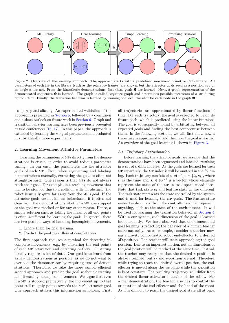
Our proposed approach consists of three stages as de-picted in Figure 2. In the first stage, the goal parametersof the individual mps are learned from the demonstrationdata (Section 2). In the second stage, a representation ofthe demonstrated sequences is learned by connecting theobserved mps in a graph (Section 3). Each node in thegraph corresponds to a mp and each transition leads toa potentially succeeding mp. In the final stage, the mp

transition behavior is learned (Section 4). One classifier islinked to each node in the graph. The task of the classifieris to decide when to transition to a new state in the graphduring the reproduction of a skill, resulting in an activationof a different mp. These decisions are made based on thecurrent state of the robot and its environment. The stateis based on a set of features which are computed fromraw sensor values. The graph structure therefore helpsto improve the classification, as the overall classificationproblem is split into many smaller problems which may beeasier to solve. Here, the reduced difficulty is due to the re-striction of the possible classification results, which leads to

2

MP Library

[

x

y

]

=

[

23

]

[

x]

=[

1]

[

α]

=[

0◦]

Goal Learning Graph Learning Switching Behavior

❶ ❷ ❸

Figure 2: Overview of the learning approach. The approach starts with a predefined movement primitive (mp) library. Allparameters of each mp in the library (such as the reference frames) are known, but the attractor goals such as a position x/y oran angle α are not. From the kinesthetic demonstrations, first these goals ❶ are learned. Next, a graph representation of thedemonstrated sequences ❷ is learned. The graph is called sequence graph and determines possible successors of a mp duringreproduction. Finally, the transition behavior is learned by training one local classifier for each node in the graph ❸.

less perceptual aliasing. An experimental validation of theapproach is presented in Section 5, followed by a conclusionand a short outlook on future work in Section 6. Graph andtransition behavior learning have been previously presentedat two conferences [16, 17]. In this paper, the approach isextended by learning the mp goal parameters and evaluatedin substantially more experiments.

2. Learning Movement Primitive Parameters

Learning the parameters of mps directly from the demon-strations is crucial in order to avoid tedious parametertuning. In our case, the parameters are the attractorgoals of each mp. Even when segmenting and labelingdemonstrations manually, extracting the goals is often notstraightforward. One reason is that mps do not alwaysreach their goal. For example, in a reaching movement thathas to be stopped due to a collision with an obstacle, therobot is usually quite far away from the mp’s goal. If theattractor goals are not known beforehand, it is often notclear from the demonstrations whether a mp was stoppedas the goal was reached or for any other reason. Hence, asimple solution such as taking the mean of all end pointsis often insufficient for learning the goals. In general, thereare two possible ways of handling incomplete movements.

1. Ignore them for goal learning.

2. Predict the goal regardless of completeness.

The first approach requires a method for detecting in-complete movements, e.g., by clustering the end pointsof each mp activation and detecting outliers. Clusteringusually requires a lot of data. Our goal is to learn fromas few demonstrations as possible, as we do not want tooverload the demonstrator by requiring tens of demon-strations. Therefore, we take the more sample efficientsecond approach and predict the goal without detectingand discarding incomplete movements. We argue that evenif a mp is stopped prematurely, the movement up to thatpoint still roughly points towards the mp’s attractor goal.Our approach utilizes this information as follows. First,

all trajectories are approximated by linear functions oftime. For each trajectory, the goal is expected to lie on itsfuture path, which is predicted using the linear functions.The goal is subsequently found by arbitrating between allexpected goals and finding the best compromise betweenthem. In the following sections, we will first show how atrajectory is approximated and then how the goal is learned.An overview of the goal learning is shown in Figure 3.

2.1. Trajectory Approximation

Before learning the attractor goals, we assume that thedemonstrations have been segmented and labelled, resultingin a set of k different mps. As the goals are learned for eachmp separately, the mp index k will be omitted in the follow-ing. Each trajectory consists of a set of pairs {ti, si}, whereti is the time and si ∈ R

q×1 is a vector whose elementsrepresent the state of the mp in task space coordinates.Note that task state si and feature state xi are different.The task state represents the state controlled by the systemand is used for learning the mp goals. The feature stateinstead is decoupled from the controller and can representanything, such as the state of the environment. It willbe used for learning the transition behavior in Section 4.Within our system, each dimension of the goal is learnedindependently. We have observed that one-dimensionalgoal learning is reflecting the behavior of a human teachermore naturally. As an example, consider a teacher mov-ing a gravity compensated robot end-effector to a desired3D-position. The teacher will start approaching the goalposition. Due to an imperfect motion, not all dimensions ofthe goal position will be reached at the same time. Instead,the teacher may recognize that the desired x-position isalready reached, but y- and z-position are not. Therefore,while trying to reach the desired overall position, the end-effector is moved along the yz-plane while the x-positionis kept constant. The resulting trajectory will differ fromthe desired linear attractor behavior of the robot. Fora real demonstration, the teacher also has to control theorientation of the end-effector and the hand of the robot.As it is difficult to reach the desired goal state all at once,

3

0 100 200 3001.2

1.4

1.6

Raw Time

Task

State

s

(a) Trajectory

0 0.1 0.2 0.31.2

1.4

1.6

Normalized Time

Task

State

s

(b) Normalization

0 0.2 0.4 0.6 0.81.2

1.4

1.6

Normalized Time

PredictedState

s

(c) Approximation and Prediction

1.2 1.4 1.60

2

4

6

8·10−2

Predicted State s

CostsJ(s)

(d) Goal Learning

Figure 3: Goal learning overview. The trajectories (a) are velocity normalized (b) and approximated by linear functions (solid redlines, c). For each trajectory, the goal is expected to lie on its future path (red dashed lines), which is predicted using the linearfunctions. The goal (thick black line) is then found by minimizing the cost function (d), which arbitrates between all expectedgoals. Note that the cost function is zero for the entire gray area. Therefore the center of the interval is chosen as goal of the mp.The thin black line shows the mean of the trajectory end points as comparison.

humans seem to concentrate on a few dimensions first.Therefore, demonstrations usually do not really match theattractor behavior of a real robot motion. To compensatefor this mismatch, we learn the goal per dimension. In thefollowing, we therefore use a scalar notation for the taskspace.

We focus on tasks where the velocity of a movement isirrelevant. Therefore, the time does not correspond to thereal time axis of the demonstrations, but is computed bynormalizing the velocity

ti = ti−1 + (si − si−1)2, t0 = 0, (1)

as illustrated in the two left plots in Figure 3. As model forthe approximation of a trajectory, a simple linear functionis used

f(ti) = ati + b = si. (2)

Here, si is the predicted state of the mp at time ti anda and b are the parameters of the model. Although alinear function is a simple model, it is notable here thatit matches the demonstrations of single attractor move-ments quite well, as they can be seen as point-to-pointmovements in task space. We focus on tasks that havesuch linear characteristics, e.g., pick-and-place tasks. Theassumption of a linear model usually does not apply for thetransition between two mps. During demonstration andreproduction of a sequence, a transition can occur with anon-zero velocity. As a consequence, the start of a mp maybe influenced by its predecessor. The resulting trajectorywill contain arcs or edges and is an example for a trajec-tory that cannot be well represented using a straight line.Nevertheless, note that there is no need to approximatethe whole trajectory well in our approach. Instead, theline only has to pass through the real goal at some futuretime point. The method has to find the parameters ofEquation (2) to ensure this property.

Therefore, we chose to use weighted least squares re-gression (wlsr, [5]) for learning the parameters a and b.

Compared to least squares regression, wlsr additionallyallows to weight the importance of each data point. Byweighting the data points at the end of a trajectory strongerthan at the beginning, it is possible to minimize the in-fluence of the preceding movement, while still matchingthe overall trajectory well. The parameters are found byminimizing the weighted sum of distances between the sam-pled states si and predicted states si from Equation (2),resulting in the cost function

J(a, b) =

N∑

i=1

g(i) (si − si)2. (3)

Here, N is the number of samples and g(i) is a weightingfunction. We suggest to use g(i) = i2/N , as the quadraticweights minimize the influence of the preceding mp at thestart of a trajectory and focus on the data points closer tothe goal. Cubic or even larger weights focus on few datapoints at the end of a trajectory and therefore becomesensitive to noise. Minimizing the error function (3) isstraightforward (see [5]).

2.2. Goal Learning

We assume that a mp has been active M times, result-ing in M trajectories approximated by linear functions fjwith j = {1, . . . ,M}. Figure 3(c-d) shows an overview ofour goal learning approach. As already mentioned, thebasic idea is that for each trajectory j, the goal is expectedto lie on its future path. The future path is predicted usingthe linear function fj , which allows us to formulate theexpected goal in terms of the slope parameter aj and thepredicted state uj at the final time of the trajectory

uj = fj(t(j)N ). (4)

If the slope is positive, the expected goal is equal or greaterthan uj . If it is negative, the expected goal is equal orless than uj . For finding the best compromise between all

4

State s

Distancesdj

State s

Distancesdj

Time

Task

State

s

Time

Task

State

s

Time

Task

State

s

State s

Distancesdj

State s

CostsJ(s)

State sCostsJ(s)

State s

CostsJ(s)

Figure 4: Three goal learning cases and their resulting distanceand cost functions. In general, trajectories may converge (top),diverge (center) or point in the same direction (bottom). Theblack dashed lines show the goal of the mp.

trajectories, we construct a cost function which penalizesdeviations from each expected goal. As a first step, wedefine the distance between a state s and the expected goalof a trajectory j as

dj(s) =

0, if aj > 0 and s ≥ uj ,

0, if aj < 0 and s ≤ uj ,

|s− uj | , otherwise.

(5)

Then, the attractor goal of one particular dimension of amp can be defined as the point sg where the squared sumof distances becomes minimal

J(s) =

M∑

j=1

d2j (s), (6)

sg = mins

J(s). (7)

Figure 4 shows some trajectories and their resulting dis-tance and cost functions as an example. For finding thesolution sg, we first calculate the derivative of the costfunction (6). Due to Equation (5), the cost function isnon-differentiable at each threshold uj . Therefore, thederivative has to be computed for each interval [uj , uj+1]separately and is given by

d

dsJ(s) = 2

∑

j∈D

(s− uj). (8)

Here, D is the set of functions for which Equation (5) isnon-zero. For the intervals, we assumed that the thresholdshave been sorted in ascending or descending order. Settingthe derivative equal to zero and rearranging for s results in

sg =1

nD

∑

j∈D

uj , (9)

where nD is the number of elements in D. The solution sgmay lie outside of the interval. In that case, it is clippedto the closest interval border. If there exists an interval forwhich D is empty, the error will become zero and henceany value in this interval is a possible solution. In thatcase, the center of the interval is taken as goal. The finalequation therefore is

sg =

(uj + uj+1)/2 if nD = 0,

uj if nD 6= 0, sg < uj ,

uj+1 if nD 6= 0, sg > uj+1,

sg otherwise.

(10)

The goal sg is computed for every interval [uj , uj+1] andsubsequently inserted into Equation (6). The goal resultingin the lowest value of this cost function is then chosen asfinal goal of the mp.

Due to the quadratic dependency of Equation (6) onthe expected goals, overshoots may shift the goal awayfrom the desired value. However, our experience is that ifa teacher recognizes that the goal was not hit accurately,he/she usually corrects his/her mistake, so that in the endthe real goal is approximately reached. If a mp is stoppedprematurely, overshoots also do not lead to problems. Ad-ditionally, the trajectory approximation with wlsr leadsto some robustness against overshoots.

3. Learning Graph Representations

In the previous section, the parameters of the individ-ual mps have been acquired. In this section, we proposean approach for learning a graph representation of thedemonstrated sequences which we call sequence graph. Ina sequence graph, every node is linked to a mp. Duringreproduction, the graph determines which mp may be acti-vated next. A missing transition in the graph might preventan activation of the correct mp, while too many outgoingtransitions might lead to the activation of a wrong mp dueto perceptual aliasing. It is therefore crucial to find a goodstructure for a given set of demonstrations.

Figure 5 shows an overview of the graph learning basedon a simple toy example with only three different mps,that will be used throughout this section. The mps areindicated by different colors. They are chosen arbitrarilyand have no further meaning, but show the essential char-acteristics of our approach. First, we perform at least onekinesthetic demonstration. In general, we assume that Mdemonstrations have been collected. For each demonstra-tion, we get a labeled (background colors in Figure 5a) setof features (black lines). The features are only used forlearning the transition behavior and will be explained inSection 4. For learning a sequence graph, only the observedmp sequence is used, as shown in Figure 5b. The graphrepresentation will be explained in detail in the followingsection, where we also present two different types of se-quence graphs, both showing different ways of incorporatingthe sequences into the representation.

5

0 25 60 85 110 140 175 220 2500

0.2

0.4

0.6

0.8

1

Sample

Fea

ture

Value

(a)

25 60 85

110

140175220

(b)

25

220

60,110

175 85,140

(c)

25 60,110

175

85,140

220

(d)

Figure 5: Overview of the graph learning. First, the labeled data from a set of demonstrations (a) is taken to extract the mp

sequence (b). This sequence can then be used to generate a sequence graph. We investigate two different sequence graph types. Acompact local sequence graph (c) and a more sophisticated global sequence graph (d). The numbers on the transitions correspondto the transitions points (tps, see upper left figure). A tp is a point in time at which a transition between mps occurs.

A sequence graph is a directed graph in which eachnode ni is linked to a mp. This mapping is not injectivewhich means a mp can be linked to more than one node.During reproduction, a mp is activated if a linked nodeis considered active. Transitions in the graph lead to suc-ceeding mps that can be activated if the current mp hasfinished. A transition tk,l is connecting the node nk with nl.Each transition is linked with the corresponding transitionpoints (tp) at which it was observed during the demon-stration (black vertical lines in Figure 5a). As the sametransition can be observed multiple times, multiple tps arepossible.

Having m nodes in a graph, we use a m×m transitionmatrix T with elements tk,l to describe one sequence graph.As a mp is usually activated for more than one time step,the transition tk,k exists for all k. We start with onedirected acyclic graph with nodes nj,i for each trial (seeFigure 5b), which contains the observed mp sequence. Themain step is now to combine multiple of these graphsinto one representation of the skill, which can be a hardproblem as the algorithm has to work solely based on theobservations. As an example, consider the task of bakinga cake. Here, it does not matter if milk or eggs are putin the bowl first. Still, the task may be demonstrated onetime with the sequence milk-eggs and one time with thesequence eggs-milk. From an algorithmic point of view itis often not clear if a sequence is arbitrary for a skill orif the differences can be linked to some traceable sensorevents. Hence, there are different ways of building thegraph structure for a skill. We show two possibilities byinvestigating two different kinds of sequence graphs. Thelocal graph presumes a sequence to be arbitrary and is notconsidering it in the representation, while the global graphis trying to construct a more detailed skill description.

3.1. Local Sequence Graph

The local sequence graph assigns exactly one node toeach activated mp and hence the number of nodes and mpsis equal. The graph is initialized with one node per mp

and without transitions. For each observed pair of mpsa transition is added to the graph. As only pairs and nohistory are considered, it is irrelevant at which point in thesequence a transition occurs. The corresponding graph forthe toy example is shown in Figure 5c.

The graph contains only three nodes, one for each acti-vated mp. When reproducing the movement, a transitionfrom the red mp to the blue one is always possible at thislevel of the hierarchy and it is up to the classifier to preventsuch incorrect transitions. The major drawback of thisrepresentation is the strong requirement on the feature set,as it has to be sufficiently meaningful to allow for a correctclassification independent of the history of activated mps.

3.2. Global Sequence Graph

The global sequence graph attempts to overcome thisissue by constructing a more detailed skill description. Oneessential characteristic of the global sequence graph is thatthere is no one to one mapping between mps and graphstates. Instead, a mp can appear multiple times in one rep-resentation as depicted in the global sequence graph of thetoy example (Figure 5d). Here, two nodes are linked to thered mp because the sequence was considered to be in twodifferent states when they were activated. The repeatedappearance of the green-blue transitions (see Figure 5a) isrepresented by only two nodes as in the local graph. Thereason is that consecutive sequences of the same mps areconsidered to be a repetition which can be demonstratedand reproduced an arbitrary number of times. Repeti-tions are also advantageous when describing tasks with

6

Algorithm 1 Graph Folding

Require: T

1: repetition = findRepetition(T );2: while repetition.found do

3: R = ∅;4: repetition.l = repetition.end − repetition.start + 1;5: for i = repetition.start to repetition.end do

6: mergeNodes(T (i+ repetition.l),T (i));7: R = R ∪ T (i);8: repetition = findRepetition(T );9: if !repetition.found then

10: tail = findTail(T , repetition.end + 1);11: if tail .found then // Found incomplete cycle12: for i = tail .start to tail .end do

13: mergeNodes(T (i+ r),T (i));14: R = R ∪ T (i);15: T = T \R; // Remove merged nodes from graph

repetitive characteristics, such as unscrewing a light bulb.Here, the unscrewing movement has to be repeated severaltimes depending on how firm the bulb is in the holder.As the number of repetitions is not fixed for each singledemonstration, the algorithm has to conclude that differentnumbers of repetitions of the same behavior appeared inthe demonstrations and incorporate this information intothe final representation of the task.

Note that even if a skill requires a fixed number ofrepetitions, both presented sequence graphs will containa cycle in the representation. The system is then onlyable to reproduce the movement properly if the classifierwould find the transition leading out of the cycle afterthe correct number of repetitions. While an improvementis not possible here for the local graph, a fixed numberof repetitions can be modeled with the global graph byskipping the search for cyclic transitions.

3.3. Graph Construction

The local sequence graph is created by adding one nodefor each observed mp and one transition for every observedmp pair. If a mp pair is observed multiple times, only onetransition is added to the graph. For creating a globalsequence graph, three steps have to be performed.

1. Create one acyclic graph T j for each demonstration.

2. Replace repetitions of mps with cyclic transitions.

3. Combine updated graphs to one global representationT of the skill.

The first step is straightforward as the acyclic graph rep-resents the mp sequence directly observed in the demon-strations. We call the second point folding and its pseudocode is shown in Algorithm 1. The algorithm starts bycalling the method findRepetition, which is searching forrepetitions of length l = ⌊m/2⌋ in a graph T with mnodes. The method starts by comparing the mps of thenodes {n0, n1, . . . , nl} with {nl+1, . . . , n2l+1}. If both node

Algorithm 2 Graph Merging

Require: TA, TB

1: UA = getUniquePaths(TA);2: UB = getUniquePaths(TB);3: for all uB ∈ UB do // Iterate over paths4: cmax = 0;5: for all uA ∈ UA do

6: c = compare(uA,uB); // Nr. matching nodes7: if c > cmax then

8: cmax = c;9: nB,max = uB(1, . . . , c); // First c nodes

10: nA,max = uA(1, . . . , c);11: for all nA ∈ TA, nB ∈ TB do // Iterate over all nodes12: if nB ∈ nB,max then // Nodes match13: mergeNodes(nA, nB);14: else // Node of graph B has to be added to A15: addNode(TA, nB);

chains match, the node pairs {n0, nl+1} . . . {nl, n2l+1} arereturned. If the chains do not match, the indices are incre-mented by one and the method starts from the beginningwith n1 as starting point. The shifting is done until the endof the list is reached. Next, l is decremented by one andall previous steps are repeated. Thus, longer repetitionsare preferred over shorter ones. The method terminates ifthe cycle size is one, which means no more cycles can befound.

If a repetition is found, the corresponding nodes aremerged to a single node. When merging two nodes nA andnB, the input and output transitions of node nB becomeinput and output transitions of nA. If an equal transitionalready exists for nA, only the associated tps are addedto the existing transition. Note that a cyclic transition isintroduced when merging the nodes n0 and nl+1, as thisleads to the input transition tl,l+1 being rerouted to tl,0.After each iteration of the algorithm, the nodes of the latterchain are not connected to the rest of the graph anymoreand can be removed from the representation. To allowescaping a cycle not only at the end of a repetition, thealgorithm also searches for an incomplete cycle after a foundrepetition. This tail is considered to be part of the cycleand is also merged into the cyclic structure (Algorithm 1,lines 11-15). The toy example also contains an incompletecycle, as the green-blue repetitions end incompletely withthe green mp.

We call the final step of creating a global sequencegraph merging, as several separate graphs are merged intoone representation. Algorithm 2 merges two graphs andthus gets called M − 1 times for M demonstrations. Thealgorithm steps through the graphs simultaneously, startingat the initial nodes, merging equal nodes and introducingbranches whenever nodes differ. The algorithm starts byextracting the unique paths from both graphs. A uniquepath is a path which starts with a node that has no inputtransition and ends with a node that has either no output

7

85,140

60 85 1100

0.2

0.4

0.6

0.8

1

Sample

Featu

reValue

110 140 1750

0.2

0.4

0.6

0.8

1

Sample

(a)

0 0.1 0.2 0.3 0.4 0.5 0.6 0.7 0.8 0.9 10

0.2

0.4

0.6

0.8

1

Feature Predecessor ( )

Featu

reSuccessor(

)

(b)

Figure 6: One classifier is created for each node in the graph. The training is performed by using the data around the transitionsbetween the connected mps (a). The data is projected into feature space and the classifier learns a separating border between themps, as indicated by the background color in (b). As soon as the current feature state crosses such a border during reproduction, atransition in the graph is triggered, leading to a switch to a different classifier.

transition or only output transitions to nodes that werealready visited. The toy example has two unique paths,red, green, blue and red, green, red, blue (see Figure 5d).Next, the algorithm compares the paths of both graphswith each other from left to right, searching for the longestequal subpath. Two nodes are considered as equal if thecolumns of the corresponding transition matrices are equal,which means both nodes use the same underlying mp andhave the same input transitions. Finally, the nodes ofthe longest equal subpath are merged, whereas all othernodes of graph TB are added to TA. By searching forthe longest subpath, branches are introduced at the latestpossible point in the combined graph. Once branched, bothbranches are separated and do not get merged together ata later point in the sequence.

4. Learning the Transition Behavior

After creating the graph representation, the next stepis to train the classifiers — one for each node in the graph.If a node is active during reproduction, its associatedclassifier decides when to transition to a possible succes-sor node. This multiclass classification problem has theactive node and all of its neighbor nodes in the graphas classes. Due to the graph representation, we do nothave to learn an overall classification function f(x) = pwith p ∈ P and x being the combined feature vector ofall mps x = (x(1); x(2); . . . ; x(K))T, but can restrict theclasses c of each classifier to a subset Pc ⊆ P and the datavector to the feature vectors of the elements in Pc. Restrict-ing the number of classes often increases the accuracy of thesystem as transitions not observed in the training data areprevented. A reduction of the feature vector can be seenas an implicit dimensionality reduction where unimportantfeatures used by uninvolved mps are no longer consideredfor the decision.

Figure 6a depicts the data used for training a classifieras an example. After the demonstrations, each transitionin the acyclic graph is linked to one tp in the sampleddata. During the merging and folding process of the global

sequence graph or the pair search for the local graph transi-tions are merged together, resulting in potentially multipletps for each transition. For each tp, the data points be-tween the previous and next tp in the overall data aretaken from the training and labeled with the mp that wasactive during that time. As all transitions have the samepredecessor for one classifier, the first part of the data willalways have the same labels, while the second part maydiffer depending on the successor node of the transition.

The classifiers learn from the labeled training data howto separate the mps in feature space (Figure 6b). Duringthe reproduction of the mp, the current feature state of therobot is tracked and as soon as it crosses a border, the corre-sponding successor will be activated, leading to a transitionin the graph and a switch to another classifier. Any classifieris applicable to our method. We evaluated support vectormachines (svms, [8]), logistic regression (lr, [2]), kernellogistic regression (klr, [8]), import vector machines (ivms,a certain type of sparse kernel logistic regression, [30]), andGaussian mixture models (gmms, [2]).

5. Evaluations and Experiments

For evaluating our approach, we perform three differentexperiments. In Section 5.1, we evaluate the goal learn-ing on a task where a robot has to move an object in itsworkspace. In Section 5.2, we evaluate the overall perfor-mance of the system, including the two sequence graphrepresentations and different classifiers. In the experiment,a robot has to unscrew a light bulb. In Section 5.3, thesystem has to learn to grasp different objects. Addition-ally, an error recovery strategy for unsuccessful grasps isdemonstrated. With the third experiment, we evaluate thesystem performance on a more complex feature set. Allexperiments are evaluated using a real seven degrees offreedom (dof) Barrett wam robot with an attached fourdof hand. For the first and third experiment, also somesimulation results are presented.

8

Figure 7: In the first experiment, the robot has to move an objectto a certain position. The robot starts in an initial position ( ),moves to the object ( ) and grasps it ( ). Subsequently, itmoves the object to another position ( ), opens its hand ( )and moves to the final position ( ).

5.1. Moving an Object

The first experiment evaluates the goal learning algo-rithm we describe in Section 2. Therefore, we chose arather simple sequence of movements, which does not differbetween single demonstrations. The robot starts in aninitial position, moves to the object and grasps it. Subse-quently, it moves the object to another position, opens thehand and returns to the initial position, as illustrated inFigure 7. As the sequence always is the same and does notinclude any repetitions or specific patterns of movements,the local and global sequence graph algorithms return thesame structure. A mp may control the position and/ororientation of the end effector as well as the joint anglesof the fingers. If an entity is not controlled by a mp, themovement results from the null space criteria (e.g., jointlimit avoidance) of the underlying task space controller.Six different mps have been defined to perform the task, asshown in Table 1.

Before the experiments on the real robot are presented,the goal learning is evaluated in simulation first. As kines-thetic teaching is not possible in simulation, we predefinethe demonstrated sequence with a state machine and thetransition behavior between mps using thresholds. For re-alism and variation, Gaussian noise is added to the thresh-olds. Every time a new mp is activated, new thresholdsare computed. The goal of each mp k is set to desiredvalues s

(k)g and perturbed with additive noise N (0, σ2

I)for each demonstration. The intention of this experiment isto evaluate the robustness and accuracy of the goal learningby disturbing the transition behavior and mp goals. Weperform eight demonstrations with a fixed σ and learn the

goals s(k)g of every mp k after each demonstration with the

data of all demonstrations that have been performed up tothis point. For each learning instance, an error is computed

MP Position Orientation Fingers Next MP Initial - -

A Fixed Open

Hold Fixed Closed

B Fixed Closed

Hold Fixed Open

Final - - -

Table 1: mps for the object movement experiments.

1 2 3 4 5 6 7 8

2

4

6

8·10−2

Number of Demonstrations

Error

σ = 0.05 σ = 0.03 σ = 0.01

Figure 8: Goal learning error for the simulated toy example.The error degrades when demonstrating a task multiple times.The background color shows the hull of one standard deviation.

according to

e =1

N

N∑

k=1

∥

∥

∥s(k)g − s

(k)g

∥

∥

∥

1, (11)

which is the mean of the ℓ1-norm of the difference betweenpredefined and computed goal of all N mps. The experi-ment is repeated with three different values for σ 20 times,so that in total 480 demonstrations are performed. Wesummarize the results for all learning instances accordingto the number of demonstrations they have been trainedwith and compute the mean and standard deviations ofthe errors. The results are plotted in Figure 8. In general,the error decreases slightly for more demonstrations, butis always consistent with the amount of noise added to thesystem.

For the experiments with the real robot, we performthree kinesthetic demonstrations. Transitions between mpsare indicated by pressing a key every time we consider amovement as complete. Opening and closing of the hand isalso activated by pressing a key. The labeling is performedbased on the indicated transitions. Next, the transitionbehavior is learned with svms as classifier and the task isreproduced on the real robot.

One feature x(k)1 is assigned to each mp k according to

the equation

∆ = s(k)g − s

(k), (12)

x(k)1 = 1− exp(−0.5(∆TΣ−1

k ∆)). (13)

Here, s(k) ∈ Rq×1 is the current state of the robot in task

space coordinates and Σk is a q × q diagonal matrix withpositive parameters. Note that q can be different for eachmp. Equation (13) depends on the absolute differencebetween the state of the robot and the mp’s goal position.Hence, the feature can be seen as progress indicator and iscalled goal distance [14]. It is intrinsically in the range [0, 1]and makes further data scaling superfluous. In addition, thevariation of the feature around the mp goal can be shapedwith the parameters of Σk. To get expressive features, welearn the parameters by minimizing the variance of thefeature values while constraining the min and max valuesto be as close to zero and one as possible.

9

0.9 0.95 1 1.05 1.1

1.06

1.08

1.1

1.12

1.14

Normalized Time

Positionz

Active mp

(a)

2.6 2.8 3 3.2 3.41.08

1.1

1.12

1.14

Normalized Time

Positiony

Active mp

(b)

3.6 3.8 4 4.2 4.41.55

1.6

1.65

1.7

Normalized Time

Orien

tationEulerβ

Active mp

(c)

Figure 9: Comparison of trajectories from kinesthetic demonstrations (blue) and reproduction (red). The dashed lines show thelearned mp attractor goals. All trajectories are aligned in time, so that each mp activation takes the same (normalized) time. Thelearned goals and the transition behavior are consistent with the demonstrations.

Figure 10: Illustration of a successful unscrewing sequence. The robot starts in an initial position ( ) and first moves towards thebulb ( ). Then it repeats the unscrewing movement ( , , , ) until the bulb loosens ( ) and subsequently, the bulb is put intoa bin ( ) and the robot returns to its initial position ( ).

Figure 9 shows the resulting trajectories for some se-lected mp transitions. The learned goals are consistentwith the directions of the movements. If trajectories areconstant or diverge slightly, the goal is averaging over thetrajectories (Figures 9b,c). If all trajectories point in thesame direction as it is the case for Figure 9a, the goallies in this direction as well, without conflicting with thetrajectories.

The first example also illustrates the difference betweenthe goal state of a mp and the state at which a new mp

is activated. A new mp is activated as soon as the clas-sification border is crossed, which is the case when thefeature state reaches the value of the first transition. Notethat such an early transitioning strategy is only triggeredif it was also demonstrated. Therefore, behaviors such asopening or closing a gripper prematurely should not occurunintendedly.

5.2. Unscrewing a Light Bulb

In the second experiment, the system has to learn howto unscrew a light bulb. The focus of this experiment is onevaluating the overall performance of the learning system,including the goal learning, the graph representations andthe transition behavior. For the representation of the skill,we choose seven different mps, shown in Table 2.

The detailed task flow is illustrated in Figure 10. Wechoose to unscrew the light bulb by caging it. Here, therobot encloses the bulb with its hand and grasps it belowthe point with the largest diameter. For positioning therobot, the end effector coordinates defined relative to thelight bulb holder are set. When opening, closing or rotating

the hand, either the three dofs of the fingers or the angleof the wrist joint are controlled by the mp. The unscrewingmp (rotating the closed hand counterclockwise) additionallyapplies a force in upward direction to the robot’s hand toensure contact with the bulb. Again, the goal distancefeature is assigned to each mp. The goal distance of the -mp can be used to detect if the light bulb is still in theholder. As a force is applied in upward direction duringunscrewing, this force leads to an acceleration of the robot’sarm as soon as the light bulb gets loose. As a consequence,the arm moves away from the mp’s goal, resulting in anincreasing value of the goal distance. The system has tolearn that an increase of this goal distance leads to animmediate stopping of the unscrewing mp and a transitionto the branch in the graph that puts the light bulb into thebin. As the light bulb is not represented in the feature setand the unscrewing stopping criterion depends implicitly onthe height of the end-effector, a slipped light bulb can notbe detected. As no slip happened during our experiments,we did not integrate the state of the light bulb into thefeature set.

MP X Y Z Orientation Fingers Next MP Initial Position Initial Hold , Light Bulb Hold Spread

Light Bulb Hold Closed

Bulb Bulb Force Rot. Wrist Closed , Light Bulb Hold Spread , Light Bulb Rot. Back Spread

Garbage Hold Closed

Table 2: mps for the light bulb experiments.

10

1 2 30

50

100

Number of Demonstrations

�Success/mp

Baseline Local Global

(a) Graph Comparison

1 2 30

50

100

Number of Demonstrations

�Success/mp

lr gmm svm ivm

(b) Classifier Comparison

Figure 11: Experimental results for the light bulb task. The left plot shows the comparison of the three different graph structures: Afully connected graph used as baseline and the local and global sequence graph. All graphs were trained with Logistic Regression (lr)as classifiers. The right plot shows the evaluation of different classifiers: lr, Gaussian Mixture Models (gmms), Support VectorMachines (svms), and Import Vector Machines (ivms). Here, the global sequence graph has been used. The bars in both plotsindicate the minimum, average and maximum success rate of each mp transition during reproduction of the task.

Initial

(a) Global Sequence Graph

Initial(b) Local Sequence Graph

Figure 12: Graph representations of the light bulb task. Com-pared to the global graph, the local graph merges several nodes.The merging creates paths in the graph which were not demon-strated. An example is the sequence marked as red which leadsto a misbehavior of the robot if reproduced.

We perform three kinesthetic demonstrations and varythe position of the light bulb holder for each demonstration.For all following experiments, the system is trained sepa-rately with the data of each single demonstration, all pairsof demonstrations and all demonstrations. Every time thesystem is trained, the task is reproduced and the successrate of each mp transition is evaluated. A transition isconsidered successful, if the system activates at the correctstate the correct successor. Incorrect, premature or toolate transitions are considered failures. For unsuccessfultransitions, we restart the movement, trigger the transitionmanually and continue with the reproduction from there.

We first evaluate the graph representations by compar-ing the local and global sequence graph with a baselinegraph, which has one node for each mp and is fully con-nected. Hence, the system is allowed to transition to anymp at every point in time. All graph types are trainedwith lr as classifiers. The reproduction results are shownin Figure 11a. Both presented graph representations areclearly better suited than the baseline graph. Due to thereduced number of outgoing transitions for each node, theeffect of perceptual aliasing gets reduced, which in turnimproves the performance of the classifiers. This effect isalso the reason why the global sequence graph slightly out-

performs the local sequence graph. Both graphs are shownin Figure 12. The local sequence graph contains pathswhich have not been demonstrated and lead to misbehaviorif reproduced. An example is the red path in the figure.Here, the robot returns to its initial position with the bulbin its hand and immediately goes back to the bulb holderwhile opening its hand instead of going to the bin.

In a second set of experiments, we evaluate differentclassifiers. In addition to lr, we evaluate gmms, svms,and ivms (see Section 4). All classifiers are trained withthe global sequence graph, as this was the overall winnerof the first experiments. The reproduction results for thedifferent classifiers are shown in Figure 11b. The resultsindicate only a slightly better performance of the kernelmethods compared to lr and gmms. When being trainedwith all demonstrations, the average success rate of svmsand ivms is 97.6%, while lr reaches only 92.9%. The mainreason for failing is the unscrewing movement, where thesystem sometimes fails to generalize from the demonstra-tions. When the light bulb gets loose at the beginningof the unscrewing movement during demonstration, thesystem is expected to be in a similar state when the lightbulb gets loose during reproduction. If both states aredifferent, the system sometimes fails to trigger the transi-tion to the successor mp properly. This effect is reducedif more demonstrations are performed, as different wristorientations are observed for each transition and thereforethis feature becomes irrelevant for the decision. In gen-eral, a feature selection method may be helpful for furtherimproving the performance.

5.3. Grasping Objects with Error Recovery

In a third experiment, the system has to learn to graspand lift three cylinders with different lengths using differ-ent grasps. The intention is to evaluate a more complexfeature set, which also represents the state of the environ-ment, positions and joint angles instead of the mp goaldistance features. Table 3 summarizes all features for this

11

Top

Power

Pinch

Initial / Reset

Reset

Figure 13: Task flow of the grasping task. The robot starts inan initial position (top). Depending on the size of the cylinderand its orientation, the system approaches the cylinder withdifferent orientations and finger configurations. Subsequently,the cylinder is grasped and lifted. If the contact with thecylinder is lost during lifting, the system has to re-start thetask.

task. The position of the end-effector is relative to thecylinder. Inclination and rotation are angles that representthe orientation of the cylinder. Both features are illustratedin Figure 14. Orientation and position of the cylinder aremeasured using a six dof magnetic field tracking sensor sys-tem with precisions of approximately 1 cm and 0.15◦. Thestrain gauges measure the tension in each finger. Togetherwith the finger joint angles, they are used for detectingsuccessful grasps or a slipped cylinder.

The task is demonstrated as follows (see Figure 13). Theend-effector starts in an initial position and is first movedto a pre-grasp position close to the cylinder. Subsequently,the cylinder is grasped and lifted. Depending on the lengthof the cylinder and its orientation, different grasps andpre-grasps are used to solve the task. If the cylinder isstanding, it is grasped from the top. If it standing upsidedown, it is grasped at its bottom. We demonstrate thetask with three different cylinder lengths, 8, 16, and 24 cm.If the cylinder is lying and has a length of 8 or 24 cm, itis grasped using the power grasp. If the 16 cm cylinder islying, it is grasped using the pinch grasp. Pinch and powergrasp can be performed with two different wrist anglesas shown in Figure 14. During the final lifting step, the

Feature DimensionCylinder Length 1

Cylinder Inclination 1Cylinder Rotation 1

End-Effector Position 3Strain Gauges 3

Finger Joint Angles 4

Table 3: Feature set for grasping task.

α

Top Viewx

y

(a) Rotation

β

β

Side Viewx

z

(b) Inclination

Figure 14: The rotation feature (a) is the angle between theshown axes of the lying cylinder (red) and the hand (green).For avoiding unnecessary rotations of the end-effector, we definetwo pre-grasp mps that approach the cylinder with differentorientations (top and bottom). Depending on the angle α, themp that is closer to its target orientation should be activated.The feature is shown for the pinch grasp, but is used for thepower grasp in the same manner. The inclination feature (b)is the angle between the negative gravity vector (black) andthe shown cylinder axis (blue). It indicates if the cylinder isstanding (β = 0), lying or standing upside down (β = π).

cylinder may slip. In that case, the lifting is immediatelystopped. The end-effector is moved to the initial positionand the task is demonstrated from the beginning. Note thateven though this error recovery strategy is demonstrated tothe robot, the system has no explicit notation of an errorwhen reproducing the task. Instead, a slipped cylinder issupposed to lead to a mp transition which is treated justas any other mp transition. The immediate triggering ofthe error recovery is also a typical example for a mp thatis stopped before reaching its goal state when reproducingthe task.

Similar to the previous experiments, we train the systemincrementally after each demonstration. Each training isfollowed by an evaluation of the reproduction. A successfulreproduction of the tasks requires grasping and lifting thecylinder, as well as successfully detecting a slipped cylinder.Figure 15 shows the success rate of the reproduction forall 17 demonstrations. We evaluated the system with thelocal sequence graph and lr in simulation and svms onthe real robot. The results indicate that the system is ableto learn the task completely, even though more demon-strations have to be performed compared to the light bulbtask. The increased number of required demonstrationsis not surprising, as the resulting graph has six outgoingtransitions for the initial node. The transitions for the lyingcylinder depend non-linearly on the cylinder length. Thelogistic regression models fail to cover this non-linearity.As a result, usually the power grasp is performed when thecylinder is lying. Even though this might also lead to a suc-cessful grasp, it is not the behavior that was demonstratedfor the medium-length cylinder and is therefore considered

12

6 8 10 12 14 160%

20%

40%

60%

80%

100%

Demonstrations

SuccessRate

LR (simulation)

SVM

Figure 15: Reproduction results for the grasping task. Whilean accuracy of 100% can be achieved using svms, the logisticregression (lr) models fail to cover the non-linear dependencyon the length of the cylinder.

a failure. The experiment shows that the system workswell when using positions or joint angles instead of the mp

goal distances as features. It also shows that it is easyto integrate arbitrary other features into our framework,which can for example describe the state of the environ-ment. The only requirement of our system is, that thefeatures are meaningful enough, so that successive mps canbe separated well in feature space.

6. Conclusion and Future Work

In this paper, we proposed a method for learning to se-quence single movements from kinesthetic demonstrationsin order to reproduce a complex task. We showed how theparameters of the single linear attractor movements as wellas the transition behavior between the movements can belearned. Learning the transition behavior is formulatedas classification problem. We showed how mp sequencesobserved from kinesthetic demonstrations can be incorpo-rated into one graph representation we call sequence graph.A sequence graph allows to split the overall classificationproblem into many smaller problems, as it is possible tolearn the transition behavior between mps locally for eachnode in the graph. We presented two different types of se-quence graphs and evaluated four different classifiers. Theapproach was validated in three experiments using a realseven dof Barrett wam robot with a four dof hand. Theresults show that our system is able to learn the transitionbehavior from very few demonstrations.

In future work we want to investigate how an optimalsequence graph can be found, considering not only themp sequences but also the actual data sampled from thedemonstrations. Additionally, we plan to use co-activatedmps and a two-arm setup. Therefore we need methods forsynchronizing concurrently active movements.

Acknowledgment

We thank Manuel Muhlig for his help at setting up themagnetic field tracking system and his assistance duringthe experimental evaluation of the approach.

[1] Brenna D. Argall, Sonia Chernova, Manuela Veloso, and BrettBrowning. A survey of robot learning from demonstration. Robot.Auton. Syst., 57(5):469–483, 2009.

[2] Christopher M. Bishop. Pattern Recognition and Machine Learn-ing. Springer-Verlag New York, Inc., 2006.

[3] R.A. Brooks. A robust layered control system for a mobile robot.IEEE Journal of Robotics and Automation, 2(1):14–23, Mar1986.

[4] J. Butterfield, S. Osentoski, G. Jay, and O.C. Jenkins. Learningfrom demonstration using a multi-valued function regressor fortime-series data. In IEEE-RAS Int. Conf. Humanoid Robots,2010.

[5] R. J. Carroll and D. Ruppert. Transformation and Weightingin Regression. Chapman & Hall, Ltd., 1988.

[6] Guoting Chang and Dana Kulic. Robot task learning fromdemonstration using petri nets. In IEEE Int. Symp. Robot andHuman Interactive Communication, 2013.

[7] S. Chiappa and J. Peters. Movement extraction by detectingdynamics switches and repetitions. In Advances in Neural In-formation Processing Systems, 2010.

[8] Corinna Cortes and Vladimir Vapnik. Support-vector networks.Machine Learning, 20(3):273–297, 1995.

[9] S. Ekvall and D. Kragic. Learning task models from multiplehuman demonstrations. In IEEE Int. Symposium Robot andHuman Interactive Communication, pages 358–363, 2006.

[10] Tamar Flash and Binyamin Hochner. Motor primitives in ver-tebrates and invertebrates. Current Opinion in Neurobiology,15(6):660 – 666, 2005.

[11] D.H. Grollman and O.C. Jenkins. Incremental learning of sub-tasks from unsegmented demonstration. In IEEE/RSJ Int. Conf.Intelligent Robots and Systems, 2010.

[12] B. Hayes and B. Scassellati. Discovering task constraints throughobservation and active learning. In IEEE/RSJ Int. Conf. Intel-ligent Robots and Systems, 2014.

[13] Dana Kulic, Christian Ott, Dongheui Lee, Junichi Ishikawa,and Yoshihiko Nakamura. Incremental learning of full bodymotion primitives and their sequencing through human motionobservation. Int. J. Rob. Res., 31(3):330–345, 2012.

[14] T. Luksch, M. Gienger, M. Muehlig, and T. Yoshiike. Adaptivemovement sequences and predictive decisions based on hierar-chical dynamical systems. In IEEE/RSJ Int. Conf. IntelligentRobots and Systems, 2012.

[15] G.J. Maeda, M. Ewerton, R. Lioutikov, H.B. Amor, J. Peters,and G. Neumann. Learning interaction for collaborative taskswith probabilistic movement primitives. In Int. Conf. HumanoidRobots, 2014.

[16] S. Manschitz, J. Kober, M. Gienger, and J. Peters. Learn-ing to sequence movement primitives from demonstrations. InIEEE/RSJ Int. Conf. Intelligent Robots and Systems, 2014.

[17] S. Manschitz, J. Kober, M. Gienger, and J. Peters. Learning tounscrew a light bulb from demonstrations. In ISR/ROBOTIK2014, 2014.

[18] Bernard Michini. Bayesian Nonparametric Reward Learningfrom Demonstration. PhD thesis, Massachusetts Institute ofTechnology, Department of Aeronautics and Astronautics, Cam-bridge MA, August 2013.

[19] Monica N. Nicolescu and Maja J. Mataric. Natural methods forrobot task learning: Instructive demonstrations, generalizationand practice. In Int. Joint Conf. Autonomous Agents and Multi-Agent Systems, 2003.

[20] Scott Niekum, Sachin Chitta, Andrew Barto, Bhaskara Marthi,and Sarah Osentoski. Incremental semantically grounded learn-ing from demonstration. In Robotics Science and Systems, 2013.

[21] A. L. Pais, Keisuke Umezawa, Yoshihiko Nakamura, and A. Bil-lard. Learning robot skills through motion segmentation andconstraints extraction. HRI Workshop on Collaborative Manip-ulation, 2013.

[22] M. Pardowitz, R. Zollner, and R. Dillmann. Learning sequentialconstraints of tasks from user demonstrations. In IEEE-RASInt. Conf. Humanoid Robots, 2005.

[23] P. Pastor, M. Kalakrishnan, L. Righetti, L. Righetti, and

13

S. Schaal. Towards associative skill memories. In IEEE-RASInt. Conf. Humanoid Robots, 2012.

[24] Vladimir Pavlovic, James M. Rehg, and John Maccormick. Learn-ing switching linear models of human motion. In Advances inNeural Information Processing Systems, volume 13. MIT Press,2000.

[25] Jan Peters. Machine learning of motor skills for robotics. USCTechnical Report, pages 05–867, 2005.

[26] S. Schaal, S. Kotosaka, and D. Sternad. Nonlinear dynami-cal systems as movement primitives. In IEEE-RAS Int. Conf.Humanoid Robots, 2000.

[27] F. Stulp, L. Herlant, A. Hoarau, and G. Raiola. Simultaneouson-line discovery and improvement of robotic skill options. InIEEE/RSJ Int. Conf. Intelligent Robots and Systems, 2014.

[28] M. Tenorth and M. Beetz. A unified representation for reasoningabout robot actions, processes, and their effects on objects. InIEEE/RSJ Int. Conf. Intelligent Robots and Systems, 2012.

[29] Steven D. Whitehead and Dana H. Ballard. Learning to perceiveand act by trial and error. Machine Learning, 7(1):45–83, 1991.

[30] Ji Zhu and Trevor Hastie. Kernel logistic regression and the im-port vector machine. In Journal of Computational and GraphicalStatistics, pages 1081–1088. MIT Press, 2001.

Simon Manschitz studied Information and Sys-tems Technology and received his bachelor’s andmaster’s degree from TU Darmstadt, Germany.Since 2014, he works in a joint project of theIntelligent Autonomous Systems group of the TUDarmstadt and the Honda Research Institute Eu-rope in Offenbach, Germany, as a PhD student.

Jens Kober is an assistant professor at the DelftCenter for Systems and Control, TU Delft, TheNetherlands. He worked as a postdoctoral scholarjointly at the CoR-Lab, Bielefeld University, Ger-many and at the Honda Research Institute Eu-rope, Germany. He received his PhD in 2012 fromTU Darmstadt, Germany. From 2007-2012 he wasworking at the Department Scholkopf, MPI forIntelligent Systems, Germany. He has been a vis-iting research student at the Advanced Telecom-munication Research (ATR) Center, Japan andan intern at Disney Research Pittsburgh, USA.

Michael Gienger received the diploma degree inMechanical Engineering from the Technical Uni-versity of Munich, Germany, in 1998. From 1998to 2003, he was research assistant at the Instituteof Applied Mechanics of the TUM, addressingissues in design and realization of biped robots.He received his Ph.D. degree with a dissertationon “Design and Realization of a Biped WalkingRobot”. After this, Michael Gienger joined theHonda Research Institute Europe in Germany in2003. Currently he works as a principal scientistin the field of robotics. His research interestsinclude mechatronics, robotics, control systems,imitation learning and cognitive systems. He alsoserves as a scientific coordinator for the ResearchInstitute for Cognition and Robotics (CoR-Lab)of the Bielefeld University.

Jan Peters is a full professor (W3) for IntelligentAutonomous Systems at the Computer ScienceDepartment of the Technische Universitat Darm-stadt and at the same time a senior researchscientist and group leader at the Max-Planck In-stitute for Intelligent Systems, where he heads theinterdepartmental Robot Learning Group. JanPeters has received the Dick Volz Best 2007 USPhD Thesis Runner Up Award, the Robotics:Science & Systems - Early Career Spotlight, theINNS Young Investigator Award, and the IEEERobotics & Automation Society’s Early CareerAward. Jan Peters has studied Computer Science,Electrical, Mechanical and Control Engineeringat TU Munich and FernUni Hagen in Germany,at the National University of Singapore (NUS)and the University of Southern California (USC).He has received four Master’s degrees in thesedisciplines as well as a Computer Science PhDfrom USC. Jan Peters has performed researchin Germany at DLR, TU Munich and the MaxPlanck Institute for Biological Cybernetics (in ad-dition to the institutions above), in Japan at theAdvanced Telecommunication Research Center(ATR), at USC and at both NUS and SiemensAdvanced Engineering in Singapore.

14