Embed Size (px)
Citation preview
Learning with Reproducing Kernel Hilbert Spaces:
Stochastic Gradient Descent
and Laplacian Estimation
Loucas Pillaud-Vivien
Under the supervision of Francis Bachand Alessandro Rudi
ENS - Inria Paris - PSL
2020

This is a fucking blank sentence.
2

Maths et Poésie,Pour les unes, tu trouves et ça commence,
Pour l’autre, tu trouves et ça nit.
— Marc Yor : “Les Unes et l’autre”
3

Abstract
Machine Learning has received a lot of attention during the last two decades both from industry fordata-driven decision problems and from the scientic community in general. This recent attention iscertainly due to its ability to eciently solve a wide class of high-dimensional problems with fast and easy-to-implement algorithms. What is the type of problems machine learning tackles ? Generally speaking,answering this question requires to divide it into two distinct topics: supervised and unsupervised learning.The rst one aims to infer relationships between a phenomenon one seeks to predict and “explanatory”variables leveraging supervised information. On the contrary, the second one does not need any supervisionand aims at extracting some structure, information or signicant features of the variables.
These two main directions nd an echo in this thesis. On the one hand, the supervised learningpart theoretically studies the cornerstone of all optimization techniques for these problems: stochasticgradient methods. For their versatility, they are the workhorses of the recent success of ML. However,despite their simplicity, their eciency is not yet fully understood. Establishing some properties of thisalgorithm is one of the two important questions of this thesis. On the other hand, the part concerned withunsupervised learning is more problem-specic: we design an algorithm to nd reduced order models inphysically-based dynamics addressing an crucial question in computational statistical physics (also calledmolecular dynamics).
Even if the two problems are of dierent nature, these two directions share an important feature:they leverage the use of Reproducing Kernel Hilbert Spaces, which have two nice properties: (i) theynaturally adapt to this stochastic framework on a computational-friendly manner, (ii) they display a greatexpressivity as a class of test functions.
More precisely, the rst contribution of this thesis is to prove the exponential convergence of stochasticgradient descent of the binary test loss in the case where the classication task is well specied. Thiswork establishes also ne theoretical bounds on stochastic gradient descent in reproducing kernel Hilbertspaces that are a result on their own.
The second contribution focuses on optimality of stochastic gradient descent in the non-parametricsetting for regression problems. Remarkably, this work is the rst to show that multiple passes over thedata allow to reach optimality in certain cases where the Bayes optimum is hard to approximate. Thiswork tries to reconcile theory and practice as common knowledge on stochastic gradient descent alwaysstated that one pass over the data is optimal.
In computational statistical physics as in Machine Learning, the question of nding low-dimensionalrepresentations (main degrees of freedom) is crucial. This is the question tackled by the third contributionof this thesis. We show, more precisely, how it is possible to estimate the Poincaré constant of a distributionthrough samples of it. Then, we exploit this estimate to design an algorithm looking for reaction coordinateswhich are the cornerstones of accelerating dynamics in the context of molecular dynamics.
Detailing, rening and improving this result is the forth contribution of this manuscript. This currentwork is still not completely nished, but gives some deeper theoretical and empirical insights on thediusion operator estimation. It was therefore natural that it should be part of this thesis.
Keywords: stochastic approximation, supervised learning, non-parametric estimation, reproducingkernel Hilbert spaces, dimensionality reduction, Langevin dynamics, Poincaré inequality.
4

Résumé
L’apprentissage automatique a reçu beaucoup d’attention au cours des deux dernières décennies, à lafois de la part de l’industrie pour des problèmes de décision basés sur des données et de la communautéscientique en général. Cette attention récente est certainement due à sa capacité à résoudre ecacementune large classe de problèmes en grande dimension grâce à des algorithmes rapides et faciles à mettre enoeuvre. Plus spéciquement, quel est le type de problèmes abordés par l’apprentissage automatique ? D’unemanière générale, répondre à cette question nécessite de le diviser en deux thèmes distincts: l’apprentissagesupervisé et l’apprentissage non supervisé. Le premier vise à déduire des relations entre un phénomène quel’on cherche à prédire et des variables “explicatives” exploitant des informations qui ont fait l’objet d’unesupervision. Au contraire, la seconde ne nécessite aucune supervision et son but principal est de parvenir àextraire une structure, des informations ou des caractéristiques importantes relative aux données.
Ces deux axes principaux trouvent un écho dans cette thèse. Dans un premier temps, la partieconcernant l’apprentissage supervisé étudie théoriquement la pierre angulaire de toutes les techniquesd’optimisation liées à ces problèmes: les méthodes de gradient stochastique. Grâce à leur polyvalence,elles participent largement au récent succès de l’apprentissage. Cependant, malgré leur simplicité, leurecacité n’est pas encore pleinement comprise. L’étude de certaines propriétés de cet algorithme est l’unedes deux questions importantes de cette thèse. Dand un second temps, la partie consacrée à l’apprentissagenon supervisé est liée à un problème plus spécique : nous concevons dans cette étude un algorithmepour trouver des modèles réduits pour des dynamiques empruntées à la physique. Cette partie aborde unequestion cruciale en physique statistique computationnelle (également appelée dynamique moléculaire).
Même si les deux problèmes sont de nature diérente, ces deux directions partagent une caractéristiquecommune : elles tirent parti de l’utilisation d’espaces à noyau reproduisant, qui possèdent deux propriétésessentielles : (i) ils s’adaptent naturellement au cadre stochastique tout en préservant une certaine ecaciténumérique, (ii) ils montrent une grande expressivité en tant que classe de fonctions de test.
La première contribution de cette thèse est de montrer la convergence exponentielle de la descente degradient stochastique pour la perte binaire dans le cas où la tâche de classication est “facile”. Ce travailétablit également des bornes théoriques nes sur la descente de gradient stochastique dans les espaces ànoyau reproduisant, ce qui peut être considéré comme un résultat en lui-même.
La deuxième contribution se concentre sur l’optimalité de la descente de gradient stochastique dans lecadre non paramétrique pour des problèmes de régression. Plus précisément, ce travail est le premier àmontrer que de multiples passages sur les données permettent d’atteindre l’optimalité dans certains cas oùl’optimum de Bayes est dicile à approcher. Ce travail tente de réconcilier la théorie et la pratique car lestravaux actuels sur la descente de gradient stochastique ont toujours montré qu’il susait d’un passagesur les données.
En physique statistique computationnelle comme en apprentissage automatique, la question de trouverdes représentations de faible dimension (principaux degrés de liberté) est cruciale. Telle est la questionabordée par la troisième contribution de cette thèse. Nous montrons plus précisément comment il estpossible d’estimer la constante de Poincaré d’une distribution à travers des échantillons de celle-ci. Ensuite,nous exploitons cette estimation pour concevoir un algorithme à la recherche de coordonnées de réactionqui sont les pierres angulaires des techniques d’accélération dans le contexte de la dynamique moléculaire.
Détailler, aner et améliorer ce résultat est la quatrième contribution de ce manuscrit. Ce travailactuel n’est pas encore complètement terminé, mais il donne de la profondeur aux analyses théorique etempirique de l’estimation des opérateurs de diusion. Il était donc naturel qu’il fasse partie de cette thèse.
Mots-clés: approximation stochastique, apprentissage supervisé, estimation non-paramétrique, espacesà noyau reproduisant, réduction de dimension, dynamique de Langevin, inégalité de Poincaré.
5

Contents
I Introduction 13
1 ML framework 14
1.1 General Framework of statistical learning . . . . . . . . . . . . . . . . . . . . . . . . . . . 141.2 Why we use optimization in ML . . . . . . . . . . . . . . . . . . . . . . . . . . . . . . . . 201.3 Solving the Least-squares problem . . . . . . . . . . . . . . . . . . . . . . . . . . . . . . . 26
2 Stochastic gradient descent 29
2.1 Setting . . . . . . . . . . . . . . . . . . . . . . . . . . . . . . . . . . . . . . . . . . . . . . 292.2 SGD as a Markov chain and continuous time limit . . . . . . . . . . . . . . . . . . . . . . 312.3 Analysis of SGD in the ML setting . . . . . . . . . . . . . . . . . . . . . . . . . . . . . . . 35
3 Reproducing Kernel Hilbert Spaces 38
3.1 Denition - Construction - Examples . . . . . . . . . . . . . . . . . . . . . . . . . . . . . 383.2 The versatility of RKHS . . . . . . . . . . . . . . . . . . . . . . . . . . . . . . . . . . . . . 423.3 Promise and pitfalls of kernels in ML . . . . . . . . . . . . . . . . . . . . . . . . . . . . . 46
4 Langevin Dynamics 50
4.1 What is Langevin Dynamics ? . . . . . . . . . . . . . . . . . . . . . . . . . . . . . . . . . 504.2 Sampling with Langevin dynamics . . . . . . . . . . . . . . . . . . . . . . . . . . . . . . . 524.3 The metastability problem . . . . . . . . . . . . . . . . . . . . . . . . . . . . . . . . . . . 54
II Non-parametric Stochastic Gradient descent 58
1 Exponential convergence of testing error for stochastic gradient methods 60
1.1 Introduction . . . . . . . . . . . . . . . . . . . . . . . . . . . . . . . . . . . . . . . . . . . 601.2 Problem Set-up . . . . . . . . . . . . . . . . . . . . . . . . . . . . . . . . . . . . . . . . . 611.3 Concrete Examples and Related Work . . . . . . . . . . . . . . . . . . . . . . . . . . . . . 631.4 Stochastic Gradient descent . . . . . . . . . . . . . . . . . . . . . . . . . . . . . . . . . . . 641.5 Exponentially Convergent SGD for Classication error . . . . . . . . . . . . . . . . . . . 681.6 Conclusion . . . . . . . . . . . . . . . . . . . . . . . . . . . . . . . . . . . . . . . . . . . . 69
A Appendix of Exponential convergence of testing error for stochastic gra-
dient descent 71
A.1 Experiments . . . . . . . . . . . . . . . . . . . . . . . . . . . . . . . . . . . . . . . . . . . 71A.2 Probabilistic lemmas . . . . . . . . . . . . . . . . . . . . . . . . . . . . . . . . . . . . . . 73A.3 From H to 0-1 loss . . . . . . . . . . . . . . . . . . . . . . . . . . . . . . . . . . . . . . . . 74A.4 Exponential rates for Kernel Ridge Regression . . . . . . . . . . . . . . . . . . . . . . . . 75A.5 Proofs and additional results about concrete examples . . . . . . . . . . . . . . . . . . . . 77A.6 Preliminaries for Stochastic Gradient Descent . . . . . . . . . . . . . . . . . . . . . . . . 80A.7 Proof of stochastic gradient descent results . . . . . . . . . . . . . . . . . . . . . . . . . . 81A.8 Exponentially convergent SGD for classication error . . . . . . . . . . . . . . . . . . . . 91A.9 Extension of Corollary 1 and Theorem 4 for the full averaged case. . . . . . . . . . . . . . 93A.10 Convergence rate under weaker margin assumption . . . . . . . . . . . . . . . . . . . . . 97
6
2 Statistical Optimality of SGD on Hard Learning Problems through Mul-
tiple Passes 100
2.1 Introduction . . . . . . . . . . . . . . . . . . . . . . . . . . . . . . . . . . . . . . . . . . . 1002.2 Least-squares regression in nite dimension . . . . . . . . . . . . . . . . . . . . . . . . . 1012.3 Averaged SGD with multiple passes . . . . . . . . . . . . . . . . . . . . . . . . . . . . . . 1032.4 Application to kernel methods . . . . . . . . . . . . . . . . . . . . . . . . . . . . . . . . . 1042.5 Experiments . . . . . . . . . . . . . . . . . . . . . . . . . . . . . . . . . . . . . . . . . . . 1062.6 Conclusion . . . . . . . . . . . . . . . . . . . . . . . . . . . . . . . . . . . . . . . . . . . . 108
B Appendix of Statistical Optimality of SGD on Hard Learning Problems
through Multiple Passes 110
B.1 A general result for the SGD variance term . . . . . . . . . . . . . . . . . . . . . . . . . . 110B.2 Proof sketch for Theorem 8 . . . . . . . . . . . . . . . . . . . . . . . . . . . . . . . . . . . 114B.3 Bounding the deviation between SGD and batch gradient descent . . . . . . . . . . . . . 115B.4 Convergence of batch gradient descent . . . . . . . . . . . . . . . . . . . . . . . . . . . . 117B.5 Experiments with dierent sampling . . . . . . . . . . . . . . . . . . . . . . . . . . . . . 128
III Statistical estimation of Laplacian 132
1 Statistical estimation of the Poincaré constant and application to sam-
pling multimodal distributions 134
1.1 Introduction . . . . . . . . . . . . . . . . . . . . . . . . . . . . . . . . . . . . . . . . . . . 1341.2 Poincaré Inequalities . . . . . . . . . . . . . . . . . . . . . . . . . . . . . . . . . . . . . . 1351.3 Statistical Estimation of the Poincaré Constant . . . . . . . . . . . . . . . . . . . . . . . . 1371.4 Learning a Reaction Coordinate . . . . . . . . . . . . . . . . . . . . . . . . . . . . . . . . 1401.5 Numerical experiments . . . . . . . . . . . . . . . . . . . . . . . . . . . . . . . . . . . . . 1421.6 Conclusion and Perspectives . . . . . . . . . . . . . . . . . . . . . . . . . . . . . . . . . . 144
C Appendix of Statistical estimation of the Poincaré constant and applica-
tion to sampling multimodal distributions 145
C.1 Proofs of Proposition 11 and 12 . . . . . . . . . . . . . . . . . . . . . . . . . . . . . . . . 145C.2 Analysis of the bias: convergence of the regularized Poincaré constant to the true one . . 146C.3 Technical inequalities . . . . . . . . . . . . . . . . . . . . . . . . . . . . . . . . . . . . . . 150C.4 Calculation of the bias in the Gaussian case . . . . . . . . . . . . . . . . . . . . . . . . . . 154
2 Statistical estimation of Laplacian and application to dimensionality re-
duction 164
2.1 Introduction . . . . . . . . . . . . . . . . . . . . . . . . . . . . . . . . . . . . . . . . . . . 1642.2 Diusion operator . . . . . . . . . . . . . . . . . . . . . . . . . . . . . . . . . . . . . . . . 1652.3 Approximation of the diusion operator in the RKHS . . . . . . . . . . . . . . . . . . . . 1662.4 Analysis of the estimator . . . . . . . . . . . . . . . . . . . . . . . . . . . . . . . . . . . . 1712.5 Conclusion and further thoughts . . . . . . . . . . . . . . . . . . . . . . . . . . . . . . . . 174
IV Conclusion and future work 176
1 Summary of the thesis 176
2 Perspectives 177
7

Contributions
and thesis outline
Part I. This manuscript is based on the publications that were accepted during this thesis. Hence, asignicant eort in the writing of this manuscript has been spent in this Part. It introduces the main ideasand questions that we will address in the rest of the manuscript. This introduction has two main purposes.First, this part sets the stage for the rest of the thesis by justifying its framework, the use of stochasticgradient descent, RKHS and the study of Langevin dynamics. Secondly, and perhaps more importantly, itgives a personal point of view on the topics under study and denes what are the main interests and fociof future research.
Part II. This Part gathers two results for the non-parametric stochastic gradient descent in two dierentsettings:
• SGD for classication. Here, we consider binary classication problems with positive denitekernels and square loss, and study the convergence rates of stochastic gradient methods. Weshow that while the excess testing loss (squared loss) converges slowly to zero as the number ofobservations (and thus iterations) goes to innity, the testing error (classication error) convergesexponentially fast if low-noise conditions are assumed.
• SGD for the Least-squares problem. We consider stochastic gradient descent (SGD) for least-squares regression with potentially several passes over the data. While several passes have beenwidely reported to perform practically better in terms of predictive performance on unseen data,the existing theoretical analysis of SGD suggests that a single pass is statistically optimal. Whilethis is true for low-dimensional easy problems, we show that for hard problems, multiple passeslead to statistically optimal predictions while single pass does not; we also show that in these hardmodels, the optimal number of passes over the data increases with sample size. In order to dene thenotion of hardness and show that our predictive performances are optimal, we consider potentiallyinnite-dimensional models and notions typically associated to kernel methods, namely, the decayof eigenvalues of the covariance matrix of the features and the complexity of the optimal predictoras measured through the covariance matrix. We illustrate our results on synthetic experiments withnon-linear kernel methods and on a classical benchmark with a linear model.
Part III. In this part we propose a way to estimate Laplacian operators through Poincaré inequalities.Poincaré inequalities are ubiquitous in probability and analysis and have various applications in statistics(concentration of measure, rate of convergence of Markov chains). The Poincaré constant, for which theinequality is tight, is related to the typical convergence rate of diusions to their equilibrium measure.This part is divided in two blocks:
8

9
• Poincaré constant and reaction coordinates. We show both theoretically and experimentallythat, given suciently many samples of a measure, we can estimate its Poincaré constant. As aby-product of the estimation of the Poincaré constant, we derive an algorithm that captures a lowdimensional representation of the data by nding directions which are dicult to sample. Thesedirections are of crucial importance for sampling or in elds like molecular dynamics, where theyare called reaction coordinates. Their knowledge can leverage, with a simple conditioning step,computational bottlenecks by using importance sampling techniques.
• Laplacian Estimation and dimensionality reduction. Here, we extend the previous results onPoincaré constant estimation by proving that the same procedure gives, without additional cost, allthe spectrum of the diusion operator and not only the rst eigenvalue. This work highlights thefact that the use of positive denite kernels allows to estimate Laplacian operators with possiblycircumventing the curse of dimensionality unlike local methods –which are currently used.
Part IV. This Part concludes the thesis by summarizing our contributions and describing future directions.
Publications. Published articles related to this manuscript are listed below:
• Part II is based on two articles published during the thesis:
?? Exponential convergence of testing error for stochastic gradient methods, L. Pillaud-Vivien, A. Rudi and F. Bach, published in the Conference On Learning Theory in 2018.
?? Statistical Optimality of Stochastic Gradient Descent on Hard Learning Problems
through Multiple Passes, L. Pillaud-Vivien, A. Rudi and F. Bach, published in the Advancesin Neural Information Processing Systems in 2018.
• Part III is based on a published article and a work in preparation:
?? Statistical Estimation of the Poincaré constant and Application to Sampling Multi-
modal Distributions, L. Pillaud-Vivien, F. Bach, T. Lelievre, A. Rudi, G. Stoltz, published inthe International Conference on Articial Intelligence and Statistics in 2020.
?? Statistical estimation of Laplacian and application to dimensionality reduction,L. Pillaud-Vivien and F. Bach, in preparation, 2020.
?
? ?

Forewords
and precautions
Before the reader dives into this manuscript, I would like to take the time to write a few words about howI wanted it to be presented. Hopefully, these precautions could guide the reader throughout this work,softening its judgment and luckily putting light on several of its important features.
First, let us begin by saying that this thesis gathers the articles published during the time of PhD. Hence,as this will be the case in Part III of this thesis, several unsolved questions may be stated as assumptions inone part and showed later. This approach is deliberate: the will behind this manuscript is to restore whathas been done in this thesis, both its questions and its evolution. This is the reason why we decided toleave Part III, Section 2 as an unnished contribution and preferred to explain the main ideas behind whathas to be nished rather than writing a self-contained complete project omitting important pieces of thewhole story. In this context, the only newly written contributions of this thesis are the introduction, theconclusion and the discussion conducted in the nal Section of the thesis (Part III, Section 2).
Second, let me comment briey on how the introduction has been thought of. Besides, as tradition, recallingthe context of this thesis including the general ML framework in supervised learning or the presentationof the less-known dynamics studied in statistical physics, we have tried to think of this introduction as anatural story that has lead us to the studies involved in Part II and III. This is the reason why a particularattention has been paid to motivate deeply the use of stochastic gradient descent or reproducing kernelHilbert spaces together with their possible pitfalls and future promises. The use of transitions under theform of questions, remarks or developments concluding each subsection of the introduction is the unifyingthread of this way of thinking. The reader will certainly remark the following patterns:
?
? ?
Motivation / Transition / Conclusion / Guideline.
They are breathes in the thesis and their goals are to link, motivate and create a common story line to allthis introduction.
10

11
Going further, I would like to stress that my personal background on partial dierential equations andprobability (I had never seen a Machine Learning problem before the beginning of my thesis) drives menaturally to theoretical and modelling questions and to try as much as possible to build bridges with otherelds of applied mathematics. This is a personal inclination that hopefully will enrich my future researchand be a pleasant guide when reading this thesis.
I would also like to put a particular emphasis on the fact that all what I could say during this introductionor during further developments are personal point of views. Even though mathematical theorems are alwaystrue by their logical nature, (at least my) way of tackling a problem is always subjective and personal. Inthis thesis, I tried to motivate why certain questions have a particular relevance and why some directionsor ways to think could convince me more than others. Nonetheless, these ways of facing a problem areonly personal interpretations and do not, in any manner, claim to indisputable truth. As a matter of fact,given my young age and inexperience, I am always thrilled to change, sharpen or rene my point of viewson many subjects when convinced by good arguments.
Finally, people have often warn me that the PhD was the last moment of the academic life where wecould take the time to explore ideas freely. I truly thank my PhD advisor Francis that let me take thisfreedom. This thesis, and especially the introduction, is, in a way, the presentation of this other work that Iaccomplished during my PhD: gathering, looking into new ideas and building my own personal sensibility.
?
? ?

This is a fucking blank sentence.
12

Part I
Introduction
1 ML framework 14
1.1 General Framework of statistical learning . . . . . . . . . . . . . . . . . . . . . . . . . . . 141.2 Why we use optimization in ML . . . . . . . . . . . . . . . . . . . . . . . . . . . . . . . . 201.3 Solving the Least-squares problem . . . . . . . . . . . . . . . . . . . . . . . . . . . . . . . 26
2 Stochastic gradient descent 29
2.1 Setting . . . . . . . . . . . . . . . . . . . . . . . . . . . . . . . . . . . . . . . . . . . . . . 292.2 SGD as a Markov chain and continuous time limit . . . . . . . . . . . . . . . . . . . . . . 312.3 Analysis of SGD in the ML setting . . . . . . . . . . . . . . . . . . . . . . . . . . . . . . . 35
3 Reproducing Kernel Hilbert Spaces 38
3.1 Denition - Construction - Examples . . . . . . . . . . . . . . . . . . . . . . . . . . . . . 383.2 The versatility of RKHS . . . . . . . . . . . . . . . . . . . . . . . . . . . . . . . . . . . . . 423.3 Promise and pitfalls of kernels in ML . . . . . . . . . . . . . . . . . . . . . . . . . . . . . 46
4 Langevin Dynamics 50
4.1 What is Langevin Dynamics ? . . . . . . . . . . . . . . . . . . . . . . . . . . . . . . . . . 504.2 Sampling with Langevin dynamics . . . . . . . . . . . . . . . . . . . . . . . . . . . . . . . 524.3 The metastability problem . . . . . . . . . . . . . . . . . . . . . . . . . . . . . . . . . . . 54
13

1. ML FRAMEWORK 14
1. ML framework
In this part, we will try to introduce the main questions raised in the thesis and we will try to dene andmotivate the natural setting of this manuscript. We will begin in Section 1.1 with standard denitions,introducing the standard Machine Learning framework from the last or three two decades. Then, as this isthe main point of view of this thesis, we will show in Section 1.2 why and how optimization is of crucialimportance in common Machine Learning problems. We nally illustrate all these ideas in Section 1.3 inthe Least-squares setting.
1.1. General Framework of statistical learning
1.1.1. What is Machine Learning ?
Due to its recent successes in the industry and the phantasms associated to it, Machine Learning (ML)is nowadays often invoked every time data are concerned. However, ML is not the only eld dealingwith data: other and perhaps older applied mathematics elds such as optimization, statistics or signalprocessing have tackle numerous problems during the past decades. Obviously, ML is deeply linked to allof them, but a more interesting question is how they are related and what are the main dierences ? Whatis ML proper focus ? Considering my youth in the eld I cannot claim that I can sharply dene ML, but Iwill try to pinpoint what is my vision of it. The aim of this manuscript is to guide the reader throughoutall the questions I have ask myself during these three years and the answers I tried to give.
Let us begin with one denition: in my opinion, ML is an high-dimensional look at statistics that takethe current computational framework into account.
High-dimensionality. Because all along this thesis two important quantities related to the data will beconsidered as huge:
• The size of the samples: d. Examples such that Natural Language Processing (words), vision (pixels)or biological systems (genome) are often embedded in spaces of more that one million dimensions.
• The number of samples: n. To face the large dimensionality of the data, engineers have built hugedata bases, so that n can be also considered as large as million.
To handle well these two large numbers, we will try to focus on non-asymptotic results: this will have thebenet to stress the dependence into these two important parameters of the problem. Indeed, asymptoticresults can sometimes hide large constants preventing from clear phenomenological explanations. Notethat another way to apprehend high-dimensionality may be to give results with respect to a certainfunction of both n and d going to innity (e.g. n/d). This is not the case in this thesis. We refer to theintroduction of [Wai19] for a remarkably clear presentation of the setting of non-asymptotic statisticalanalysis.
Computational framework. We will also draw a particular attention to the computational complexityof the algorithms analyzed or designed. In ML, as both n and d can be very large, we have to takeinto account that easy mathematical expressions can be very expensive and thus very time-consumingto compute. Operations such as matrix inversion or multiplication must be avoided as they could leadto unpractical algorithms for real problems in such a high-dimensional setting. Let us add that even ifthe algorithms designed and analyzed in this thesis carry no memory issue, this could be also a seriouscomputer-related limitation for other procedures.
This being said, we now describe mathematically what is the common setting of our dierent works.

1.1. General Framework of statistical learning 15
1.1.2. Supervised learning
Distinction between supervised and unsupervised learning. Learning, as its name states, is allabout learning from the data. One piece of information that we may want to retrieve from raw data couldbe to understand its structure or extract representative and understandable features of it. In this casewe talk about unsupervised learning [STC04, HTF09]. Another task that we may want to do is to inferthe outcome of a system leveraging the access of some known input/output pairs of it. Because it oftenrequires the supervision of the system by a human being (labeling data for classication is one of the mostimportant example of this), we call this supervised learning [Vap13, SSBD14, HTF09]. Roughly speaking,Part II analyzes the workhorse algorithm of supervised learning whereas Part III designs and analyzes analgorithm for unsupervised learning tasks.
As the work of this thesis on unsupervised learning is very related to some particular task I refer toPart III and to Section 4 for the description of the mathematical setting. I now describe the mathematicalframework behind supervised learning whose versatility and wide range apply in Part II.
Supervised learning. In supervised ML, the aim is to predict output Y ∈ Y from input(s) X ∈ X
given that we have access to n input/outputs pairs (xi, yi) ∈ X× Y. The usual ML framework states thatthere exists some distribution ρ on X× Y such that (xi, yi) are independent and identically distributedaccording to ρ. Note that even if (xi, yi) are random variables, we will not use capital letters to denotethem, emphasizing on the fact that they are samples. We can here decompose the problem into two sourcesof randomness:
• Randomness in the inputs. They are given according the some law ρX (marginal of ρ along X).In this case the xed design setting arises when ρX is a sum of diracs on the xi. Note also thatunsupervised learning techniques with respect to the samples given according to ρX can be used aspre-processing on the dataset.
• Randomness in the outputs and noise model. A common modelling of the randomness in theoutputs is to write that there exists f∗ such that
Y = f∗(X) + ε (1)
where ε is the noise of the model. Hence the randomness hypothesis on the output can be insteadcast into a random noise on the model. This can be caused by mistakes in the labeling or some errorscoming from experiments when collecting the data. Note that when we assume ε independent of X ,we often say that the model is well-specied.
Remark 1 (Support of ρX )
It is really important to note that ρ carries all the information of the problem and that we do not haveaccess to it. Even nding the support of ρX is a problem in itself and a very dicult task. To understandthis, let us take the example of face recognition on images with d ∼ 106 pixels. The marginal ρX livesnaturally in the space of vectorized images Rd. However only a few images are faces and the supportρX would exactly be the sub-manifold of images constituted of faces. Sampling from this manifold isactually a very hard task and a problem in itself.
Remark 2 (Hypothesis on ρ)Making hypothesis on ρ changes dramatically the problem under study. One example already given is thedierence between the random and the xed design settings. But we can also make hypothesis on the noisethrough ρ. For example, what we can place ourselves in the interpolation regime ε = 0, correspondingto the case where the marginal along Y is a dirac in f∗(X).
Considering Eq. (1), the problem of supervised learning is to learn the function f∗. For this, quantifyingthe precision of a predictor will be necessary: this is what we do in the following section.

1.1. General Framework of statistical learning 16
1.1.3. Losses and Generalization error
Let us dene our predictor, f : this is simply is a measurable function from X to Y, we denote the set ofsuch functions M (X× Y) . Quantifying the accuracy of the output Y = f(X) is the rst task that wewant to do to try solve our model. For this we dene naturally a loss
` : ((X× Y) ,M (X× Y))→ R+, (2)
where we say that ` is a suited loss for the problem if
`((X,Y ), f) is small ⇔ f(X) is a good predictor of Y. (3)
Here, we also want our predictor to show some good performances not only on the n samples we haveaccess to but also on all the possible data coming from ρ. Hence, the good quantity to consider is the risk,also called generalization error or test error:
R(f) := E(X,Y )∼ρ [`((X,Y ), f)] . (4)
Rephrase mathematically, the aim of supervised learning is to nd f such that R(f) is the smallest possible.We will denote with the subscript “∗” the fact that we reach the minimum value or the argument thatminimize this value. We dene here the best predictor of our learning problem and the minimum riskassociated to it:
f∗ = argminf∈M(X×Y)
R(f) (5)
R∗ = R(f∗) (6)
The choice of the loss is determinant and has to be made thoroughly and according to the problem underconsideration. Besides the obvious requirement stated in (3), we will see later that other issues such as theneed of convexity or robustness will come into consideration. But rst let us stress out two importantclasses of problem and their commonly associated losses.
Regression. WhenY is some interval ofR, we call the problem regression. For this and throughout Part IIthe typical loss will be the square loss: `((X,Y ), f) =
1
2(Y − f(X))
2.
Figure 1 – Usual losses in ML
Classication. It arises when the output space is bi-nary. To set ideas, we can take Y = −1, +1. Yes-No decisions or the well-known cat and dog problemsare instances of this type of problem. To tackle this,the more natural loss is the binary loss `((X,Y ), f) =1Y 6=sign(f(X)) that penalized by 1 each time a wrongprediction in made. However, as the binary losslacks some good mathematical property (convexity,smoothness) we often use surrogates losses for theproblem: the logistic loss `((X,Y ), f) = log(1 +exp(−Y f(X))) or the hinge loss used in support vectormachines `((X,Y ), f) = max0, 1− Y f(X) [SC08].The classication problem is tackled in the Section 1 ofPart III.

1.1. General Framework of statistical learning 17
1.1.4. Choosing the space of functions: pros and cons
Bayes predictor. Now that Eq. (3) give us a good measure of how good our predictor is, we can try tosolve the problem Eq. (5). Mathematically speaking this is an innite-dimensional optimization problemover the space of measurable functions M(X× Y) which is obviously intractable as M(X× Y) is a veryhard space to apprehend. Yet, it is quite remarkable that in the case of the square loss, when X,Y aresquare-integrable real random variables, we can compute exactly the optimum: f∗ is the orthogonalprojection from X to the linear subspace of Y -measurable functions:
f∗(X) = E [Y |X] . (7)
This function is called the Bayes predictor, and even if we have a closed form in this case, it remains toapproximate it properly. Recall here that we do not have access to the joint distribution ρ but only to samplesof it. Approximating directly the Bayes predictor is possible by local averaging techniques [Tsy08] but it isvery expensive in terms of samples even if moderate dimensions. Thus it is not the path we follow duringthis thesis.
How to choose the space of function H. Recall that one of the focus of this work is to be able tocompute numerically good predictors. When dealing directly with innite dimensional spaces such asM(X× Y) or even smaller like L2(X× Y), it seems impossible to design computational-friendly routinesto solve Eq. (5). Hence, a good idea is to parametrize the space of functions by some parameter θ livingin a nite dimensional space Rs and that encodes a dictionary of functions on which we can solve theproblem Eq. (5). We call these parametric spaces H. One of the most basic yet powerful ideas is to deneH as the linear functions from Rs to R: Hφ = f | f(x) = 〈θ, φ(x)〉, θ ∈ Rs, where φ(x) is a vectorof Rs containing features of x. However this parametrization comes at a cost: when restricting all thepossible predictors to a smaller class, we may be far away from the best predictor possible. Note that φis not necessarily itself linear, and can be learned, for example using deep learning techniques [LBH15](that we will introduce in few lines). In fact, we need two ingredients to choose properly the space H ofpossible predictors:
(i) H has to make the problem (5) solvable with a computer.
(ii) H has to be large enough to approximate well the Bayes predictor. We often call this the expressivityof the function space.
Other classes of function spaces satisfy (i) and (ii) without being parametric such as Reproducing KernelHilbert Spaces (RKHS) [SS02, SC08]. As they are the core of this thesis, we decided to postpone a little bitthe description of RKHS in Section 3 of this introduction.
Another class of functions satisfying (i) and (ii) that I will only introduce are function spaces representedby Neural Networks. Their construction is not new and date back to the 60s [IL67]: they are parametricfunction spaces simply built as successive compositions of linear functions and non-linear activations (suchthat the rectied linear activation x→ max(0, x)). It is worthy to say that, from a very high-level pointof view, their ability to solve well ML problems comes from their expressivity and easy computationalframework (even if they still carry some mysteries).Remark 3 (Splines)
An example of function spaces that are not well suited for our framework, and yet can solve very well theproblem (5) are splines [Wah90]. These are function spaces dened by piece-wise polynomials. On the onehand, they show a great expressivity but are computationally demanding on the other hand (especiallyin the high-dimensional setting).

1.1. General Framework of statistical learning 18
1.1.5. Solving theMLproblem: statistical issues, overtting andminimax rates
Empirical Risk Minimization (ERM). As we already said a few times before, we do not have accessto the distribution ρ and thus to the true risk dened in Eq. (4). As we only have access to n samplesfrom ρ a good idea is to substitute the risk dened by an expectation over ρ to an expectation over theassociated empirical measure of ρ: ρn = 1
n
∑ni=1 δxi . This denes the empirical risk:
Rn(f) := E(X,Y )∼ρn [`((X,Y ), f)] =1
n
n∑i=1
`((xi, yi), f). (8)
Now we have all the tools to dene the cornerstone of supervised learning, Empirical Risk Minimization,which is simply reformulating the true problem (5) with respect to the empirical measure associated to thesamples:
fn = argminf∈H
1
n
n∑i=1
`((xi, yi), f). (9)
Remark 4 (Statistical point of view on least-squares and logistic regression)The ERM framework described above can be viewed as Maximum Likelihood Estimation (MLE) for (atleast two) statistical models on the distribution ρ.
• In the case of Gaussian linear regression, when we want to t a Gaussian of mean 〈θ,X〉 as thelaw that generated Y , the maximum likelihood estimation is exactly the least-squares empiricalrisk minimization.
• We can also cast a MLE setting to a classication problem with the logistic loss when consideringa statistical model on the joint distribution ρ such that P(Y |X, θ) = B
(exp〈θ,X〉
1+exp〈θ,X〉
), where B(p)
is a Bernoulli law with parameter p.
Note that the main dierence with our work is that we never specify a priori a statistical model on thedistribution and do not assume that the model is well-specied.
Overtting and regularization. Solving directly and perfectly the ERM in Eq. (9) seems a good idea.But, actually, there is no guarantee that solving the empirical problem will generalize well when we wantto solve the true one Eq. (5). In fact, solving perfectly without further considerations will lead to a badestimation of the true predictor. Indeed, if the space of test function is large enough one always can nd apredictor such that f(xi) = yi but generalized very poorly outside of the xi: you can picture yourself thiswith degree n Lagrange polynomials on R that will interpolate perfectly inputs and outputs but behavevery badly outside of the interpolated points. This phenomenon is known as overtting. One way to avoidthis is whether to regularize the problem by some penalty term forcing a certain regularity of the estimator(see Figure 2 for an illustration), this is an old idea in statistics that occurs for example in smoothingsplines [Gu13]. Another way to do this is to restrict the space of function to a regular one to avoid chaoticbehavior outside the dataset. Note that both approaches are in fact equivalent [HTF09].
Approximation and estimation errors. As said above, regularizing to avoid overtting is equivalentto work in a smaller and smoother space. But the smaller the space of predictors we look for the lessexpressive our model get and the more we fail to approximate the best achievable predictor f∗. To formulatethis fact more formally let us call fH the best estimator of our class of function H and fn the estimatorbased on the empirical risk. What we want to control is the excess risk, which is the best achievable riskconsidering our model. It can be decomposed into two terms:
R(fn)− R(f∗) = R(fn)− R(fH)︸ ︷︷ ︸estimation error
+ R(fH)− R(f∗)︸ ︷︷ ︸approximation error
(10)

1.1. General Framework of statistical learning 19
Figure 2 – Showing the regularization to overtting phases when decreasing the regularization parameterin a regression task. These plots come from the slides of J.-P. Vert and J. Mairal lessons on Kernel methods.
The approximation error only depends on the class of function H chosen for our problem. This is adeterministic term that gets smaller as H get bigger.
The estimation error comes from the fact that our estimator fn comes from the minimization of theempirical risk and not of the true one. In fact, one can show that we can upper bound it by a certainuniform distance between the two functions Rn (which is a random function) and R:
R(fn)− R(fH) = R(fn)− Rn(fn) + Rn(fn)− Rn(fH)︸ ︷︷ ︸60
+Rn(fH)− R(fH)
6 R(fn)− Rn(fn) + Rn(fH)− R(fH)
6 2 supf∈H
∣∣∣Rn(f)− R(f)∣∣∣ .
A little taste of empirical process theory. Bounding uniformly the deviation between R and itscorresponding average is the key point of empirical process theory [VDVW96, Tal94]. Let us now putemphasis on the fact that this kind of development is not the point of view taken in this thesis as ourestimator will come from an optimization procedure and will benet from implicit forms of regularization(see next section for more details). However, let us try to summarize what are the main ideas and resultsbehind this. An important quantity is the Rademacher complexity associated to the loss and the functionspace H. It measures richness of a class of real-valued functions with respect to a probability distribution:
Radn = Eσ,ρ
[supf∈H
(1
n
n∑i=1
σi`((xi, yi), f)
)],
where σ are i.i.d. Rademacher variables P(σi = ±1) = 1/2. We can show from a symmetrization argumentthat
E supf∈H
∣∣∣Rn(f)− R(f)∣∣∣ 6 2Radn.
Hence, controlling the Rademacher complexity allows to bound the excess error for a wide range of classesof losses and H. For examples, if the loss is L-Lipschitz, inputs are bounded by R and the functionalspace in formed of κ-bounded functions, one has Radn 6 κRL/
√n [HTF09]. Note that these bounds
could be tighten with ner assumptions using localized version of Rademacher complexities [BBM05].But, as already stated, this is not the line of search of our work as our analysis relies on direct and straightcomputations. However, I truly believe that knowing and summing up this beautiful and deeply rootedtheory of statistical learning was worth the detour and could at any point complement my point of view.
Minimax rates of convergence. Throughout the thesis, we will focus only on upper bounds of ourestimators like in the precedent paragraph. However each time we nd such an upper bound we mayimmediately ask the following questions: is the analysis tight ? Given the level of information I have onthe problem (number of samples n, a priori on ρ, level of noise...), can I build a dierent estimator willgeneralize better ? In what way is my result or my estimator impossible to improve ?
1.2. Why we use optimization in ML 20
These questions raise the fundamental concept of optimality of the result (in the sense that it cannotbe improved). Minimax rates of convergence are exactly the good mathematical tool to embrace thisconcern: they give the best possible level of precision we can reach considering the problem we have.More formally, let Θ ⊂ L2(ρX) be a space (parametric or non-parametric at this stage) of function wherea priori we expect the target function, fρ, to lie. Let M(Θ), be the associated classes of measure such thatfρ ∈ Θ. The best we know is that ρ ∈ M(Θ). Our goal is to have a lower bound on the best estimatorover the set of all the estimators En : z→ fz where z stands for the data set.
Minimaxn(Θ) := infEn
supµ∈M(Θ)
E(‖fµ − fz‖2L2(µX)
). (11)
Even if for some classical settings, such minimax bounds can be derived [Tsy08] (we refer also to Section 1.3for least-squares and Part II, Section 2 in non-parametric settings), the reader can imagine how dicultthe problem of nding such a quantity can be: we need to construct monstrous functions that are the lesslearnable ones over a class of distributions.
?? ?
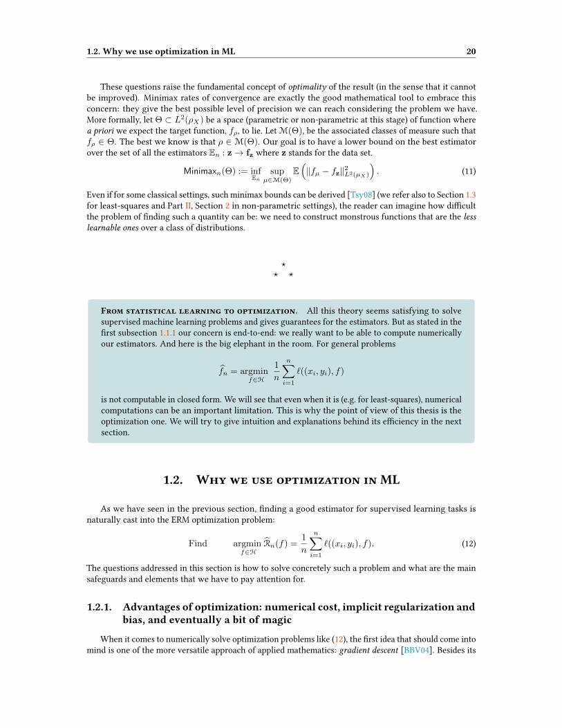
From statistical learning to optimization. All this theory seems satisfying to solvesupervised machine learning problems and gives guarantees for the estimators. But as stated in therst subsection 1.1.1 our concern is end-to-end: we really want to be able to compute numericallyour estimators. And here is the big elephant in the room. For general problems
fn = argminf∈H
1
n
n∑i=1
`((xi, yi), f)
is not computable in closed form. We will see that even when it is (e.g. for least-squares), numericalcomputations can be an important limitation. This is why the point of view of this thesis is theoptimization one. We will try to give intuition and explanations behind its eciency in the nextsection.
1.2. Why we use optimization in ML
As we have seen in the previous section, nding a good estimator for supervised learning tasks isnaturally cast into the ERM optimization problem:
Find argminf∈H
Rn(f) =1
n
n∑i=1
`((xi, yi), f). (12)
The questions addressed in this section is how to solve concretely such a problem and what are the mainsafeguards and elements that we have to pay attention for.
1.2.1. Advantages of optimization: numerical cost, implicit regularization and
bias, and eventually a bit of magic
When it comes to numerically solve optimization problems like (12), the rst idea that should come intomind is one of the more versatile approach of applied mathematics: gradient descent [BBV04]. Besides its
1.2. Why we use optimization in ML 21
simplicity, it is actually the cornerstone of (almost) all the optimization techniques used to solve supervisedlearning problems. Of course, one has to require some Hilbert structure of H and some smoothness andconvexity property to solve well this problem. However note that smoothness is not always necessary ifreplacing gradients by sub-gradients [Boy04] and that escaping from the convexity imperative might bethe next important question –we will come back to this later on.
Numerical cost. Even when the problem (12) is well posed and has a solution, there exist only a fewcases for which we can explicitly build such an estimator. Worse, as we will show later, even for oneof the simplest setting that is least-squares regression (linear space of functions with square loss): tocompute the estimator (12) requires a matrix inversion which is not compatible with our high-dimensionalcomputationally-friendly framework. On the contrary, gradient descent methods are based on a certainnumber of low cost iterations: even if there exist important variants of it as we will see in the next section,basically the cost of one iteration only requires to compute one gradient.
Versatility. As said earlier, as long as there is some Hilbert structure on the space H and some verymild assumption on the second variable of the loss `, gradient descent techniques can always be used.Computationally speaking we may add at this point that the successes of Neural Networks is partlydue to the automatic dierentiation [G+, PGC+17] (at the heart of the back-propagation in NeuralNetworks [HN92]): this is a very user-friendly framework for computing automatically derivatives andthus implementing gradient descent.
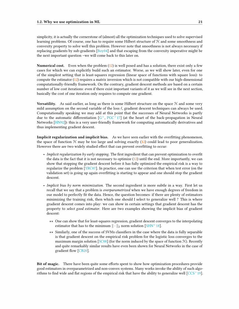
Implicit regularization and implicit bias. As we have seen earlier with the overtting phenomenon,the space of function H may be too large and solving exactly (12) could lead to poor generalization.However there are two widely studied eect that can prevent overtting to occur:
• Implicit regularization by early stopping. The rst ingredient that can prevent optimization to overtthe data is the fact that it is not necessary to optimize (12) until the end. More importantly, we canshow that stopping the gradient descent before it has fully optimized the empirical risk is a way toregularize the problem [YRC07]. In practice, one can use the criterion that when test error (on thevalidation set) is going up again overtting is starting to appear and one should stop the gradientdescent.
• Implicit bias by norm minimization. The second ingredient is more subtle in a way. First let usrecall that we say that a problem is overparametrized when we have enough degrees of freedom inour model to perfectly t the data. Hence, the question becomes: if there are plenty of estimatorsminimizing the training risk, then which one should I select to generalize well ? This is wheregradient descent comes into play: we can show in certain settings that gradient descent has theproperty to select good estimator. Here are two examples showing the implicit bias of gradientdescent:
?? One can show that for least-squares regression, gradient descent converges to the interpolatingestimator that has to the minimum ‖ · ‖2 norm solution [SHN+18].
?? Similarly, one of the success of SVMs classiers in the case where the data is fully separableis that gradient descent on the empirical risk problem for the logistic loss converges to themaximum margin solution [SC08] (for the norm induced by the space of function H). Recentlyand quite remarkably similar results have even been shown for Neural Networks in the case ofgradient ow [CB20].
Bit of magic. There have been quite some eorts spent to show how optimization procedures providegood estimators in overparametrized and non-convex systems. Many works invoke the ability of such algo-rithms to nd wide and at regions of the empirical risk that have the ability to generalize well [CCS+19].

1.2. Why we use optimization in ML 22
Figure 3 – (Left) Showing earling stopping strategy as a regularization procedure (Right) Showing max-margin eect in classication with logistic loss (Wikipedia image).
Another line of work supports that such algorithms avoid naturally bad regions and escape from localminima thanks to their momentum and/or their stochasticity. All those directions are very promising, yet,it seems that none of these ideas have fully convinced enough people to establish a form of consensus.We will conclude by saying that this is still an exciting line of research to discover what makes gradientdescent and all its variants perform so well in these tasks.
1.2.2. Gradient based algorithms: which one is the most suited for ML ?
There exists a large bestiary of gradient-based algorithms to solve optimization problems. The purposeof this section is not to give a precise and exhaustive description of such techniques but rather to give anintuition behind the use of certain algorithms. For a more mathematical perspective on such algorithms(see [BBV04] for detail analysis), we refer to subsection 1.2.3 for gradient methods and for section 2 forstochastic gradient methods.
Gradient descent algorithms. As already said all the algorithms that we will dene are based on thestandard gradient descent algorithm.
• Gradient descent. You cannot be simpler than gradient descent principle: if you want to nd theminimum of a function, just follow the line of its steepest descent. More formally, and if we usea notation that rings with risk minimization, to minimize R(θ) over θ, the gradient descent is aniterative process that chooses γt as step-size, θt=0 = θ0 at initial time and writes at times t > 0:
θt = θt−1 − γt ∇θR(θt−1). (13)
• Newton’s method. Newton method can be seen as a way to choose optimally the step-size γt. In fact,if we perform a Taylor expansion of order 2 of the function and nd the step-size that optimizesuch a local parabola, then, the optimal step-size is remarkably the inverse of the Hessian∇2R(θ).Sometimes called natural gradient in Bayesian learning, this algorithm has the nice idea to leveragethe local geometry of the function around the current iterate to speed-up the convergence.
θt = θt−1 −[∇2R(θt−1)
]−1 ∇θR(θt−1). (14)
Note that whenR(θ) is quadratic then Newton’s method converges in one iteration. Many algorithmsare inspired by this very ecient method of order two and try to approximate the inverse of theHessian (which is the bottleneck of the computation as we will see later).

1.2. Why we use optimization in ML 23
• Stochastic gradient descent and mini-batch Gradient descent. When R has a sum structure such as insupervised learning problems, it is possible to leverage this structure by taking only a minibatch Bof the whole gradient.
∇θR(θ) =1
n
∑i6n
∇θRi(θ) −→1
|B|∑i∈B∇θRi(θ).
A limit case that we will study throughout Part II of this thesis is the limit case where |B| = 1, wecan thus write with the above notation replacing R by Rt in Eq. (15):
θt = θt−1 − γt ∇θRt(θt−1). (15)
• Acceleration methods. There are dierent ways to accelerate such procedures and we will not dwellinto these techniques as they are not very relevant for this thesis. Up to my knowledge, almost everyacceleration methods boil down to adding some extra inertial term on top of the classical gradientdescent [Pol64, Nes83]. One personal remark about them: even though they can be widely used inpractice, it seems to me after many discussions with practitioners that for ML applications theycan be unstable and do not oer very dierent performances of a properly tuned basic stochasticgradient descent algorithm. However, note that acceleration can perform well in certain settings:it is the case for the randomized coordinate gradient descent as shown in [Nes12] where the onlysource of noise is multiplicative (see Section 2 of the introduction for more details).
The Bottou-Bousquet lessons. In a celebrated article [BB08], Bottou and Bousquet analyzed therelevance of the dierent algorithms presented above in the context of Machine Learning when thefunction to minimize is the population risk (yet we have only access to the empirical risk). The two mainideas given by the article have inuenced largely the optimization framework for Machine Learning in thepast decade.
• First idea: we should really be concerned about minimizing the true risk and not the training one. Thisnaive idea has the following consequence: as the train risk is not exactly the true one (typicaldistance is of order 1/
√n) it is useless optimize under a certain radius (of typical size 1/
√n).
• Second idea: for large-scale optimization, “bad” optimization algorithms can perform better. For thelarge-scale optimization framework where we are in (large n and d), some operations are very costlyto perform as recalled earlier in this thesis. Note that computing the whole gradient of the empiricalrisk cost O(nd) computing the Hessian costs the square of this price and inverting it is extremelyexpensive and unstable ! Gradient descent and Newton methods need only a few iterations toconverge but each iteration costs a lot. This is the reason why, as far a the time cost is concerned,stochastic gradient descent is preferable is such settings in comparison to full gradient descent.
1.2.3. General Optimization
The rst thing that one has to know about gradient descent is that for smooth functions it alwaysconverges to a critical point of the function to minimize. Convexity is then the good way to turn the setof critical points to global minimizers of the function. In all this section, let us call f such a function forsimplicity. Note that, as deterministic optimization is not our particular concern, all the theorems statedbelow will be stated in user-friendly settings. Note that all the hypothesis can be weakened. We refer to[BBV04] for further details on the topic.
Some denitions. Let us suppose that the function to minimize is continuously dierentiable: f ∈C1(Rd). We say that f is convex if it satises the following inequality for all x, y ∈ Rd,
f(x) > f(y) + 〈∇f(y)|x− y〉 , (16)

1.2. Why we use optimization in ML 24
which only traduces the fact that at any point x ∈ Rd the ane approximation of f is below it. Wewill also need some smoothness of the gradient (L-Lipschitz) to ensure stability of the convergence withrespect to the step-size. We say that f is L-smooth if for all x, y ∈ Rd,
‖∇f(x)−∇f(y)‖ 6 L ‖x− y‖ . (17)
Finally, we say that f is µ-strongly convex if there exists a constant µ > 0 such that for all x, y ∈ Rd,
f(x) > f(y) + 〈∇f(y)|x− y〉+µ
2‖x− y‖2, (18)
which is a stronger statement than convexity. In fact if f is twice continuously derivable all of the aboveproperties turn into Hessian conditions: (i) Convexity (16) is equivalent to ∇2f < 0, (ii) Smoothness (17)is equivalent to ∇2f 4 L and (iii) Strong convexity (18) is equivalent to ∇2f < µ. As already statedbefore, the geometry of the function f is given by its Hessian so that it seems quite natural that suchhypothesis are the cornerstone of convergence guarantees.
Gradient descent. Consider the simple optimization problem over L-smooth and convex functions fon Rd:
Find minθ∈Rd
f(θ). (19)
Let us call as usual θ∗ the unique minimizer of f (we suppose for clarity that f has a unique minimizer,note that it is true when f is strongly convex and that it does not change the idea behind gradient descentto suppose this). As said earlier gradient descent corresponds to making a step towards the steepestdirection for the ‖ · ‖2-norm. Note that changing the norm will change the direction, for example choosingthe ‖ · ‖1-norm will lead to another descent algorithm called coordinate descent. Let us recall the iterationscheme of gradient descent: it begins at θ0 and for t > 0,
θt = θt−1 − γt ∇θf(θt−1).
As Newton’s method shows, the choice of the step-size, also called learning rate in ML is of crucialimportance. For L-smooth functions, we can chose uniformly the step-size as γt = 1
L to make thealgorithm converge to the optimal solution f(θ∗), this is the meaning of the following proposition:Proposition 1 (Convergence of gradient descent)
Let f be convex and L-smooth, let γt = 1L . The sequence of gradient descent (θt)t>0 initialized at θ0
satises at time t > 0 the following inequality:
f(θt)− f(θ∗) 62L‖θ0 − θ∗‖2
t+ 4.
Moreover, if f is µ-strongly convex, we have the following upper bound:
f(θt)− f(θ∗) 6(
1− µ
L
)t(f(θ0)− f(θ∗)) .
Note that this choice of the step-size is fairly adaptive since without changing the step-size we haveacceleration from linear to exponential convergence when f is strongly convex.
Lower bound for rst order algorithms. One natural question to ask is whether this algorithmachieves the best possible rate. Is this possible to accelerate it only using gradients of the function ?Actually the answer to this question is negative, and one step forward to understand this is the fact thatusual lower bounds are faster than the rates achieved in Proposition 1. More precisely, one can designfunctions such that the convergence over all rst order methods is lower bounded by 1/t2 for convexfunction and ∼ (1−
õL )t for strongly convex ones. To tighten this lower bound, Nesterov remarkably
designed an eponymous acceleration [Nes83], this is the object of the next paragraph.
1.2. Why we use optimization in ML 25
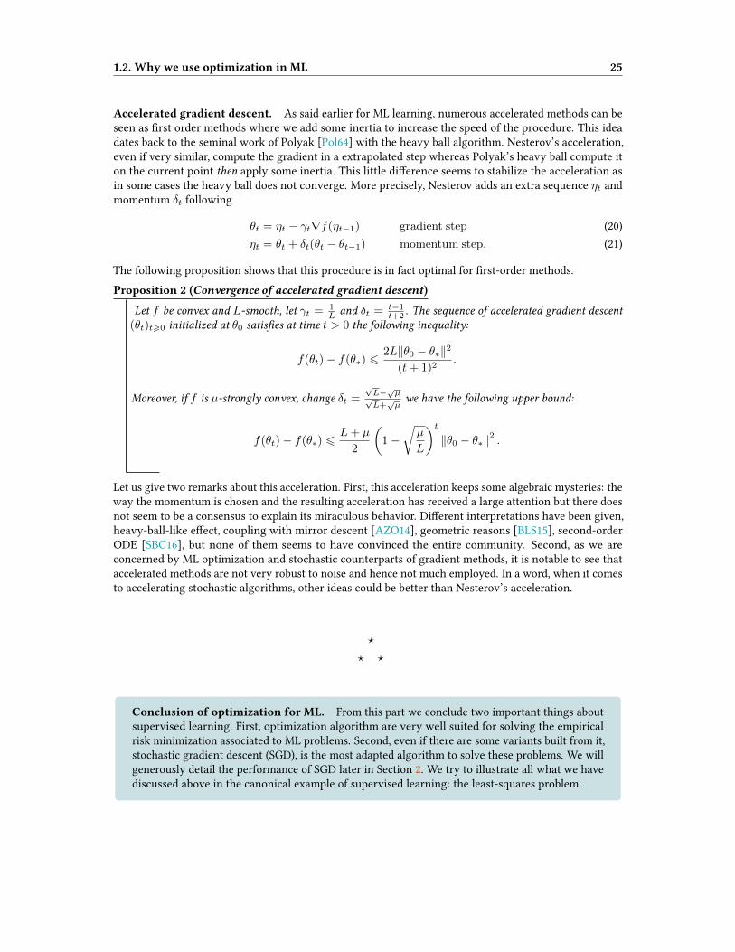
Accelerated gradient descent. As said earlier for ML learning, numerous accelerated methods can beseen as rst order methods where we add some inertia to increase the speed of the procedure. This ideadates back to the seminal work of Polyak [Pol64] with the heavy ball algorithm. Nesterov’s acceleration,even if very similar, compute the gradient in a extrapolated step whereas Polyak’s heavy ball compute iton the current point then apply some inertia. This little dierence seems to stabilize the acceleration asin some cases the heavy ball does not converge. More precisely, Nesterov adds an extra sequence ηt andmomentum δt following
θt = ηt − γt∇f(ηt−1) gradient step (20)ηt = θt + δt(θt − θt−1) momentum step. (21)
The following proposition shows that this procedure is in fact optimal for rst-order methods.Proposition 2 (Convergence of accelerated gradient descent)
Let f be convex and L-smooth, let γt = 1L and δt = t−1
t+2 . The sequence of accelerated gradient descent(θt)t>0 initialized at θ0 satises at time t > 0 the following inequality:
f(θt)− f(θ∗) 62L‖θ0 − θ∗‖2
(t+ 1)2.
Moreover, if f is µ-strongly convex, change δt =√L−√µ√L+√µwe have the following upper bound:
f(θt)− f(θ∗) 6L+ µ
2
(1−
õ
L
)t‖θ0 − θ∗‖2 .
Let us give two remarks about this acceleration. First, this acceleration keeps some algebraic mysteries: theway the momentum is chosen and the resulting acceleration has received a large attention but there doesnot seem to be a consensus to explain its miraculous behavior. Dierent interpretations have been given,heavy-ball-like eect, coupling with mirror descent [AZO14], geometric reasons [BLS15], second-orderODE [SBC16], but none of them seems to have convinced the entire community. Second, as we areconcerned by ML optimization and stochastic counterparts of gradient methods, it is notable to see thataccelerated methods are not very robust to noise and hence not much employed. In a word, when it comesto accelerating stochastic algorithms, other ideas could be better than Nesterov’s acceleration.
?
? ?
Conclusion of optimization for ML. From this part we conclude two important things aboutsupervised learning. First, optimization algorithm are very well suited for solving the empiricalrisk minimization associated to ML problems. Second, even if there are some variants built from it,stochastic gradient descent (SGD), is the most adapted algorithm to solve these problems. We willgenerously detail the performance of SGD later in Section 2. We try to illustrate all what we havediscussed above in the canonical example of supervised learning: the least-squares problem.
1.3. Solving the Least-squares problem 26
1.3. Solving the Least-sqares problem
1.3.1. Precise setting of the Least-squares problem
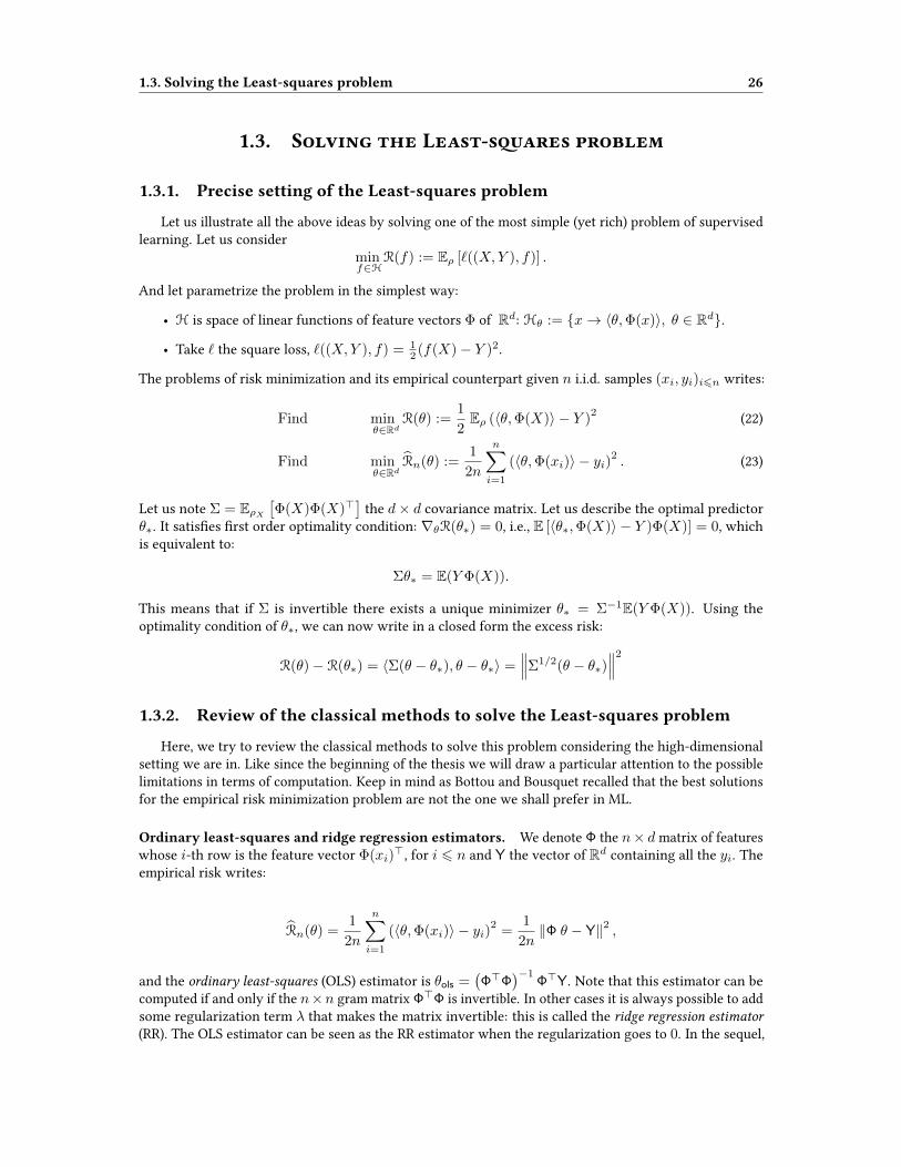
Let us illustrate all the above ideas by solving one of the most simple (yet rich) problem of supervisedlearning. Let us consider
minf∈H
R(f) := Eρ [`((X,Y ), f)] .
And let parametrize the problem in the simplest way:
• H is space of linear functions of feature vectors Φ of Rd: Hθ := x→ 〈θ,Φ(x)〉, θ ∈ Rd.
• Take ` the square loss, `((X,Y ), f) = 12 (f(X)− Y )2.
The problems of risk minimization and its empirical counterpart given n i.i.d. samples (xi, yi)i6n writes:
Find minθ∈Rd
R(θ) :=1
2Eρ (〈θ,Φ(X)〉 − Y )
2 (22)
Find minθ∈Rd
Rn(θ) :=1
2n
n∑i=1
(〈θ,Φ(xi)〉 − yi)2. (23)
Let us note Σ = EρX[Φ(X)Φ(X)>
]the d× d covariance matrix. Let us describe the optimal predictor
θ∗. It satises rst order optimality condition: ∇θR(θ∗) = 0, i.e., E [〈θ∗,Φ(X)〉 − Y )Φ(X)] = 0, whichis equivalent to:
Σθ∗ = E(Y Φ(X)).
This means that if Σ is invertible there exists a unique minimizer θ∗ = Σ−1E(Y Φ(X)). Using theoptimality condition of θ∗, we can now write in a closed form the excess risk:
R(θ)− R(θ∗) = 〈Σ(θ − θ∗), θ − θ∗〉 =∥∥∥Σ1/2(θ − θ∗)
∥∥∥2
1.3.2. Review of the classical methods to solve the Least-squares problem
Here, we try to review the classical methods to solve this problem considering the high-dimensionalsetting we are in. Like since the beginning of the thesis we will draw a particular attention to the possiblelimitations in terms of computation. Keep in mind as Bottou and Bousquet recalled that the best solutionsfor the empirical risk minimization problem are not the one we shall prefer in ML.
Ordinary least-squares and ridge regression estimators. We denote Φ the n× d matrix of featureswhose i-th row is the feature vector Φ(xi)
>, for i 6 n and Y the vector of Rd containing all the yi. Theempirical risk writes:
Rn(θ) =1
2n
n∑i=1
(〈θ,Φ(xi)〉 − yi)2=
1
2n‖Φ θ − Y‖2 ,
and the ordinary least-squares (OLS) estimator is θols =(Φ>Φ
)−1Φ>Y. Note that this estimator can be
computed if and only if the n×n gram matrix Φ>Φ is invertible. In other cases it is always possible to addsome regularization term λ that makes the matrix invertible: this is called the ridge regression estimator(RR). The OLS estimator can be seen as the RR estimator when the regularization goes to 0. In the sequel,

1.3. Solving the Least-squares problem 27
we assume that the gram matrix is invertible to avoid a deep (and certainly rich!) discussion on ridgeregression assuming that every thing behave the same in this case.
To go further, we can simplify the model without losing intuition on it by considering that thefeatures (φ(xi))i are deterministic: this is called the xed design setting. In this case, the calculations arestraightforward: θ∗ =
(Φ>Φ
)−1Φ>E [Y], Σ = 1
nΦ>Φ and denoting ε = Y − E [Y] and considering thatΦ(Φ>Φ)−1Φ> is a projector, we have
R(θols)− R(θ∗) =1
n
⟨Σ(Φ>Φ
)−1Φ>ε,
(Φ>Φ
)−1Φ>ε
⟩=
1
n
⟨Φ(Φ>Φ
)−1Φ>ε, ε
⟩=
1
ntr(
Φ(Φ>Φ
)−1Φ>εε>
).
Let suppose a isotropic noise assumption E[εε>] = σ2I , then E R(θols)− R(θ∗) = σ2rank(Φ)n , and more
generally, for uniformly bounded covariance noise, i.e., E[εε>] 4 σ2I , ER(θols)− R(θ∗) 6 σ2dn .
The last paragraph was to show the error boundO(σ2dn ) for the OLS estimator in the xed design setting.
Even in the random design setting where the (φ(xi))i are no longer deterministic, such a bound (involvingmore calculations) is still valid and is in fact optimal for this problem!. We refer to [LM+16, VDVW96] formore details. However, note that this closed form estimator requires large d, n matrix multiplications anda n× n matrix inversion which can be prohibitive for large scale problems. We will see in the two nextparagraph that gradient descent and stochastic gradient descent perform similarly but have the advantageto do it at lower cost.
Gradient descent. First we can write the gradient descent iterations to solve the empirical risk mini-mization problem. For t > 0, we simply derive the empirical risk with respect to θ,
θt = θt−1 −γtn
n∑i=1
(〈θt−1,Φ(xi)〉 − yi) Φ(xi).
This recursion corresponds to gradient descent for a strongly convex function. The main problem is thatthe strongly convex parameter controlling the exponential convergence is the smallest eigenvalue ofthe empirical covariance matrix Σn = 1
n
∑ni=1 φ(xi)φ(xi)
>, and in the large scale setting, it could beextremely small. In other words, as the matrix is badly conditioned, the exponential convergence canbe arbitrarily slow. To bypass this, a classic idea could be to regularize by some parameter λ: in thiscase the function is λ-strongly convex, but when applying gradient descent results with λ ∼ 1/n, theseapproaches fail to give exploitable bounds. On the contrary, Yao and co-authors have shown [YRC07] byearly stopping that the gradient descent performs optimally on the true risk at rate O(σ
2dn ).
As said earlier, the complexity per iteration of gradient descent is overpassed by the one of stochasticgradient descent, which is at the core of this thesis.
Stochastic gradient descent. We recall here for the subsection to be self-contained what are stochasticgradient descent iterations in this setting. Note however that this algorithm will be explained at lengthin the next section and throughout Part II. SGD follows the same principle that GD but selects only onesample to optimize instead of computing the whole sum over the dataset (that can be costly). For t > 0,the iterations read:
θt = θt−1 − γt(⟨θt−1,Φ(xi(t))
⟩− yi(t)
)Φ(xi(t)),
where i(t) ∼ U (1, . . . , n) selects uniformly at random an input/output pair in the dataset. Note thatthere are other types of sampling as the cycle sampling often used in practice that has the rule i(t) = t
mod n. Even if the complexity per iteration is very low, SGD achieves the same O(σ2dn ) error bounds
after n step [BM11].

1.3. Solving the Least-squares problem 28
Minimax rates for least-squares. Lower bounds in the case of uniformly bounded covariance of thenoise have been derived in the least-squares setting. In these works people have shown that the rateσ2dn found for our three ways to solve Empirical risk minimization is in fact optimal! We will see other
minimax rates for non-parametric settings further in this thesis in Part II, Section 2.
?
? ?
Introducing why should we use SGD. When it comes to inverting a matrix standard SVDor QR are very ecient for medium-scaled problems d 6 104. However, in large-scaled settings likein ML, gradient based algorithm are often preferred instead: indeed, solving Ax = b is equivalentto solving the optimization problem : min ‖Ax− b‖2. To solve this problem the conjugate gradientalgorithm is one of the most ecient algorithm as it is dened as the best momentum algorithmbuilt under gradient descent. Furthermore, in this setting, conjugate gradient descent has the samecomplexity as gradient descent. How to be better than such an algorithm ? For deterministicrst-order method it is impossible, but why not try stochastic versions ? This is what Strohmerand Vershynin have considered by designing the randomized Kaczmarz algorithm [SV09], whichis simply a version of importance sampling SGD for this problem. Hence, the important question:which of conjugate gradient descent and randomized Kaczmarz algorithm is better ? The answer isthat it depends on the problem at stake, and I cannot explain this better that in the seminal paper:
"It is known that the CG method may converge faster when the singular values of A are clustered.For instance, take a matrix whose singular values, all but one, are equal to one, while the remainingsingular value is very small, say 108. While this matrix is far from being well-conditioned, CGLS willnevertheless converge in only two iterations, due to the clustering of the spectrum of A. In comparison,the proposed Kaczmarz method will converge extremely slowly in this example by Theorem 3, sinceκ(A) ∼ 108 [κ is the condition number of A]. On the other hand, [the randomized Kaczmarzalgorithm] can outperform CG on problems for which CG is actually quite well suited, in particularfor random Gaussian matrices A..."
In a word, randomized gradient descent techniques can be very powerful to solve large and possiblyrandom optimization problems. They are at the core of this thesis and introduced in the nextsection.

2. STOCHASTIC GRADIENT DESCENT 29
2. Stochastic gradient descent
In the previous section we have tried to motivate why Stochastic gradient descent is nowadays theworkhorse of every large-scale ML problems. However stochastic approximations have an older historythan ML. It has been studied at rst by Robbins and Monroe in [RM51] to nd the roots of a function thatwe only have noisy measurements from. Stochastic gradient descent, in its most general denition, issimply the application of the Robbins and Monroe’s procedure the roots a the gradient of a function f .First in Section 2.1, we will describe the general setting of SGD and see that it can be exploited to analyzemany used algorithms. Then in Section 2.2 we will talk about two dierent points of view that help gettingintuition about the dynamics of SGD: see it as a Markov chain and consider a diusion associated to it.Finally, in Section 2.3, we will shortly review the known convergence results of SGD in dierent settings.
2.1. Setting
2.1.1. Stochastic approximation
We have already written the stochastic gradient descent used to minimize the empirical risk. However,let us see how SGD is dened in a more general setting. At each time t ∈ N of the procedure, let ussuppose that we only have access to an unbiased estimate of the gradient, ∇ft, of the function f we wantto minimize (it is sometimes called a rst-order oracle). More formally the unbiased esimate means thatfor a ltration (Ft)t∈N such that θt is Ft-measurable: E [∇ft(θt−1)|Ft−1] = ∇f(θt−1). Then, the SGDiterates with step-size (γt)t∈N, and initialized at θt=0 = θ0, writes
θt = θt−1 − γt∇ft(θt−1). (24)
To put the emphasis on the noise induced by the noisy estimates of the true gradient, we prefer sometimesto rephrase the recursion (24) in term of the zero-mean noise sequence εt = ∇f −∇ft.
θt = θt−1 − γt∇f(θt−1) + γtεt(θt−1).
Note that ηt := Eθt veries the classical deterministic gradient descent recursion and hence undermild assumptions, ηt converges to the minimum argument of f (as described in section 1.2.3). However,handling the variance of the recursion will necessitate two ingredients: (i) some assumptions on the noise,typically of bounded variance: E
[‖ε‖2|Ft−1
]6 σ2 (ii) assumption on the step size as we will see later in
subsection 2.3.
2.1.2. The versatility of Stochastic gradient descent
The general recursion stated in Eq. (24) can be applied to many settings, but as we have already seen,it ts particularly well in the supervised learning framework. We then briey introduce other SGD-typeprocedures particularly useful in the high-dimensional regime.
Supervised learning reformulation. We have already seen that SGD can be seen as taking only oneelement in the sum in Empirical risk minimization. However, one of the real power of SGD, as describedabove, is that it can be seen as a direct gradient method to optimize the true risk [BCN18]. Indeed, recallthat the true risk is R(θ) = Eρ `((X,Y ), θ). Now consider a input/output sample pair (xi, yi) drawn fromρ. Now, `((xi, yi), θ) is an unbiased estimate of the true risk R(θ) such that∇θ`((xi, yi), θ) is an unbiasedestimate of the true gradient of the risk. Hence, if we denote Ft = σ((xi, yi), i 6 t), then the stochasticgradient descent optimizes the true risk R(θ) as long as new points (x, y) are added in the data set.
θt = θt−1 − γt∇θ`((xt, yt), θt−1),

2.1. Setting 30
and θt is Ft-measurable. This reveals the real strength of SGD against other type of gradient descentalgorithm: as long as we consider t < n iterations, SGD optimize directly the true risk although it is an apriori unknown function. As a consequence, the SGD algorithm when t < n cannot overt the datasetand does not need any regularization.
Finite sum. As, we have already seen SGD can be seen as a stochastic optimization method thatoptimizes the empirical risk. In this case the function to minimize is Rn(θ) = E(X,Y )∼ρn [`((X,Y ), θ)] =1n
∑ni=1 `((xi, yi), θ), where ρn is the empirical measure associated to the samples ρn = 1
n
∑ni=1 δ(xi,yi).
Once again, we can derive an unbiased estimate ∇θ`((xi(t), yi(t)), θ) of the true gradient of the empiricalrisk where (i(t))t is the sequence of uniformly sampled indices over 1, . . . , n. For this, we dene theadapted ltration: Ft = σ((xk, yk)k6n, i(l)l6t). The recursion reads:
θt = θt−1 − γt∇θ`((xi(t), yi(t)), θt−1).
Note also that for this problem, a sequence of works, SAG [RSB12], SVRG [JZ13], SAGA [DBLJ14], haveshown explicit exponential convergence. However, these results, once applied to ML say nothing aboutthe loss on unseen data.
Randomized coordinate descent. Coordinate Descent (CD) [Wri15] is a popular algorithm based onpicking according to cycles one by one each coordinate of the gradient. Even if as standard SGD it reducesthe cost of computing the gradient in all the directions, some of them might be not useful to followand could represent a waste of time. This is why some randomized strategies (with possible importancesampling techniques to accelerate them) have complemented the study of Coordinate Descent. RandomizedCD [Wri15, RT14] is another example of Stochastic gradient descent. Indeed, let us minimize the functionf over Rd. Let Ft = σ(i(l)l6t) be the adapted ltration of the problem where (i(t))t is the sequence ofuniformly sampled indices over 1, . . . , d (we could replace the uniform law with other laws to resort toimportance sampling techniques), the iterations write:
θi(t)t = θ
i(t)t−1 − γt∂i(t)f(θt−1),
where ∀i 6 d, θi is the i-th coordinate of the vector θ.
Randomized Kaczmarz algorithm. We already introduced earlier in this thesis the RandomizedKaczmarz as being exactly a stochastic gradient method to solve largely overparametrized linear systems.Quite remarkably, the Randomized Kaczmarz algorithm [SV09] can be seen as the dual of randomizedcoordinate descent with proper importance sampling [Wri15, Section 1.4]. Let us simply recall it in twolines with natural ML notations. To solve the system Xθ = y, where X is a n × d matrix, θ ∈ Rd andy ∈ Rn, the idea is to solve the optimization problem: minθ ‖Xθ − y‖2 with stochastic gradient descent.Let (xi)i be the n row vectors containing X , the iterations write
θt = θt−1 −1
‖xi(t)‖2(〈xi(t), θi(t)〉 − yi(t)
)xi(t),
where i(t) = k ∈ 1, . . . , n with probability ‖xk‖2
‖A‖2 . The two main dierences with the other algorithmsabove are that the step-size γt = 1
‖xi(t)‖2and the law of i(t) are chosen according to the problem to
perform optimally.
?
? ?

2.2. SGD as a Markov chain and continuous time limit 31
A systematic analysis of random algorithms. All of these stochastic algorithms comefrom the same SGD framework described at the beginning of this section. Hence, whether weare studying SGD to minimize the true or empirical risk, whether we use randomized coordinatedescent or Karczmarz algorithm, the same general results will apply. The only dierence betweenthem is the way that we get the unbiased estimate: this can be seen mathematically in the ltrationused to dene the noise in SGD. And this could lead a systematic statistical study of SGD. Indeed,at rst order all of these algorithm are the same as their rst moment are the same: this is the SGDdenition,
E [∇Ft(θt−1)|Ft−1] = ∇f(θt−1),
where we have put a particular emphasis on the fact that F is a random variable. Note that whatmay control the speed of convergence in expectation at this point is hence the Hessian of theproblem: for example, it would be in the case of least-squares for the true risk E[XX>] andn−1
∑ni=1 xix
>i for the nite sum problem. As they share the same expectation, properties like
rates, possible acceleration can be the same. But to go deeper and study their dierence, in a veryrst-principled way of thinking of a random problem, we can look at the second moment of therandom variable:
E [∇Ft(θt−1)∇Ft(θt−1)>|Ft−1] .
This is where the multiplicative noise of SGD come from and may dier from one setting to another.
2.2. SGD as a Markov chain and continuous time limit
In this section, let us go back to the general stochastic gradient descent algorithm. In mathematicsit is always useful to understand and cast problems into known and developed theory. Indeed, whenit comes to apprehend abstract objects, mental images and representations are often the key to reallyunderstand them. We try to develop in this section two of these intuitions on SGD by giving a Markovchain interpretation of it in subsection 2.2.1 and providing a high-level comprehension of how we canmodel SGD by a continuous time diusion in subsection 2.2.2.
2.2.1. Markov chain interpretation of SGD
The rst key to understand the behavior of SGD is that when the step-size is constant, i.e. γt = γ, theiterates dene an homogeneous Markov chain [MT12]. The case where the step-size is constant is widelyused in practice as it allows to forget initial conditions rapidly. Let us recall the SGD recursion to keep itnext to us.
θt = θt−1 − γ∇f(θt−1) + γεt(θt−1).
When γ is constant, we see that SGD is a time-homogeneous Markov chain as the distribution of θtdepends only on the one of the previous iterate θt−1. What can we deduce from this point of view ? Therst thing is that under mild technical conditions, the distribution of the iterates (θt)t converges to aninvariant distribution that depends on γ and we call πγ . From this fact, we can initiate two importantreections.
(i) Closeness to θ∗. Note that our aim is to two show that (θt)t is close to θ∗. Rephrased in the Markovchain language, this is to show that the distribution of θt, call it πγ(t) is not far from the targetdistribution δθ∗ . However, we know that πγ(t) converges to πγ . Hence the question:

2.2. SGD as a Markov chain and continuous time limit 32
How far πγ is from δθ∗ ?
Giving an answer to this question is not trivial, and more importantly, it depends heavily on thenoise ε(θ). We will try to give some intuition about this question in the ML setting in the nextsubsection. For now, let us stick with some common modeling to study the recursion: make theassumption that the noise does not depend on the current iterate θ. In this case, it has been shownthat the iterates of SGD oscillates around θ∗ on a ball of radius that scales like γ1/2 [P86]. Fromthis point of view, the smaller the gamma, the closer to θ∗ we get.
(ii) The need to average. In this case, ergodic theorems for Markov chains [MT12, Section 13] giveus an important insight: they often give a way for a time-mean to converge to a deterministicquantities. As a matter of fact, under mild assumption, we can eectively show that the time-meanθt = 1
t+1
∑ti=0 θi converges to θγ = Eπγ [θ]. Furthermore, some magic happens with the quadratic
case, as we can show that θγ = θ∗: this justify the fact that throughout Part II, we will considerthe averaged SGD estimator as we have justied that almost surely θt → θ∗. However, note thatMarkov chains are not the point of view of our methods as we want to derive non-asymptotic ratesof convergence. We will prefer direct calculations instead. Note also that the same analysis can bedone in the non-quadratic case, indeed, in [DDB17] the authors showed that the order of magnitudeof the distance between θγ and θ∗ is of order γ2. This discussion is illustrated in Figure 4 taken fromthe well written thesis of A. Dieuleuveut [Die17].
Figure 4 – Stochastic Gradient Descent with constant learning rate. Dashed lines are the level lines of theobjective function f , green points correspond to the main recursion, and black to the averaged one. (Left)Quadratic case, the limit is the optimal point θ∗. (Right) General case, the limit is a dierent point θγ atdistance γ2 form θ∗.
2.2.2. Continuous time limit of SGD
Continuous time counterparts of (distrete) numerical optimization methods and Markov chain arewell-worn subject in applied mathematics.
Gradient ow. A simple example is the gradient-ow associated to the gradient descent method. Indeed,one can see the gradient descent method as a discretized approximation (called Euler scheme) with timestep ∆T = γ. More precisely, if we dene Θ some function of time t such that it corresponds togradient descent at each multiple of time γ: θn = Θ(nγ) and θn = θn−1 − γ∇f(θn−1), then for t = nγ,Θ(t+γ)−Θ(t)
γ = θn+1−θnγ = −∇f(Θ(t)) such that as γ → 0
d
dtΘ(t) = −∇f(Θ(t)). (25)

2.2. SGD as a Markov chain and continuous time limit 33
The analysis of the gradient ow (25) is already rich to understand the gradient descent. The fact that thereare no step-sizes to take care of, the use of dierential calculus and the centuries of applied mathematicsstudying such models make the analysis often more straightforward and always give powerful insights onits discretized counterpart.
Modelling stochastic gradient descent. Let us try to do the same with SGD. First recall the SGDiterations with xed step-size and i.i.d. noise. Let us suppose that the noise can be put under the formεt(θt−1) = σ(θt−1)1/2Gt, where Gt is a standard Gaussian N(0, Id) and σ(θt−1) encodes the covarianceof the noise. It writes,
θt = θt−1 − γ∇f(θt−1) + γσ(θt−1)1/2Gt. (26)
Now, a little bit of knowledge of Itô calculus and SDE discretization [KP13] will show that the noise shouldbe of scale γ1/2 to model well a diusion. This shows two things: (i) that the rst order approximationof SGD is not a diusion but the gradient ow itself (25) since the noise in SGD is too large; (ii) if wewant a second order approximation of Eq.(26), we should include γ1/2 in the covariance matrix σ(θ). Thecontinuous time diusion modelling SGD is thus:
dΘt = −∇f(Θt)dt+√γσ(Θt)
1/2dBt, (27)
where Bt is a standard Brownian motion. Note the presence of γ1/2 in the covariance of the noise of thediusion (27). In fact, in [LT19] it is shown that the SGD sequence Eq. (26) is a rst order approximationwith time-step γ of the SDE (27). Let us emphasize that two independent quantities are the same here: it isof crucial importance that both the time-step and the noise in (27) depend on γ. Even if the computationis not very complicated, this continuous time version of SGD has not been largely studied. It could bebecause diusion experts that could enlighten us are far away from the ML community. It could alsobe because the continuous time model is too dicult to study or too far from helping us building solidintuition on SGD behavior. However I really wanted to write a paragraph discussing it because it seems tome that this could be a interesting open line of research.
A toy continuous time example. To show how this continuous model can give insights about whathappen during SGD, let us illustrate this with a slight improvement of a nice example drawn from [ADT20].Consider a very simple least-squares responseless 1-d setting where we want to solve the minimizationproblem:
minθ∈R
1
2Eρ(X · θ)2,
Note that, in this case, obviously, θ∗ = 0 and there is no noise at optimum. We say that the noiseis purely multiplicative. Assume that the moment of order 4 of X exists and denote V = E[X2] andV2 = Var[X2]1/2. For samples x1, . . . , xn distributed according to ρ, the SGD recursion writes
θn = θn−1 − γx2nθn−1 =
n∏i=1
(1− γx2
i
)θ0 6
n∏i=1
exp(−γx2
i
)θ0 = exp
(−γ
n∑i=1
x2i
)θ0 ∼ e−γV nθ0,
where we used that for large n, at the rst order,∑ni=1 x
2i ∼ V n, by the law of large numbers. Obviously,
the sequence of estimators (θn)n converges to 0 exponentially fast at rate γV (at least in expectationfrom which the approximation is exact). Now, let us see what gives the continuous time SGD (27). Wehave εt(θ) = ∇f − ∇ft = (V − x2
t )θ whose square root of (co)variance (matrix) is σ(Θt)1/2 = V2θ.
Following (27), the SGD-SDE writes:
dΘt = −VΘtdt+√γV2ΘtdBt.
The acute reader will certainly recognize a geometric Brownian motion for which a close form solutioncan be written along the whole trajectory. From this, we can infer the expectation E[Θt] = Θ0e
−V t andthe variance Var[Θt] = Θ2
0e−2V t(eγV
22 t − 1). Two conclusions can be drawn from this modelling:

2.2. SGD as a Markov chain and continuous time limit 34
(i) Convergence in expectation. With the equivalence t = γn we nd the exact same rate ofconvergence e−V t for the two models.
(ii) Fluctuations. Remarkably, we can go further: if γ 6 2VV 22
, the variance of the continuous model willgo to zero exponentially fast. And with a precise look of the uctuations in the SGD iterates, wecan certainly write an expression similar to Var[Θt] showing that at the uctuation level the twosystem match! Note the important fact that in this case, the law of SGD converges to a degeneratedistribution: δθ∗=0 and does not oscillate as predicted with the Markov chain model.
Note also here that the fact that the noise depends on Θ (through its covariance) is absolutely fundamentalto see the convergence to θ∗. Indeed, if we model the noise without this θ-dependence (additive noiseperspective), one gets the following diusion:
dΘt = −VΘtdt+√γV2dBt,
which is the well-known Ornstein-Uhlenbeck process: it converges to a Gaussian law of mean 0 and ofvariance γ e
−V V 22
2V . Hence Θt will oscillate around zero on a typical ball of radius √γ like described in theprecedent paragraph when we modeled SGD by a Markov chain! Note also that the quantity γV 2
2
2V seems togovern, in any case, the behavior of the algorithm.
?
? ?
Modelling SGD: a noise issue. To conclude, we hope that we convinced the reader that theSDE model is a very good approximation to SGD recursion and that for ML settings, the noise inSGD can depend strongly on the iterates θ. This last fact changes dramatically the behavior of thealgorithm as illustrated in Figure 5.
0.4 0.2 0.0 0.2 0.4 0.6 0.8 1.0
0.4
0.2
0.0
0.2
0.4
0.6
0.8
1.0 Ornstein-UhlenbeckSGDGeometric Brownian
0.0
0.3
0.6
0.9
1.2
1.5
1.8
2.1
2.4
Figure 5 – Comparison of the dierent trajectories for the SGD diusion models. In this case ρ is theuniform distribution over the square [0, 1]2. The color map shows the value of the function to optimize.

2.3. Analysis of SGD in the ML setting 35
2.3. Analysis of SGD in the ML setting
2.3.1. Properties of SGD in the ML setting
Before stating the known results for the convergence of Stochastic Gradient Descent in dierentsettings let us briey explore further certain properties of SGD in the ML setting. First, recall that thegeneral SGD recursion can be written under the following form
θt = θt−1 − γ(∇f(θt−1) + εt(θt−1)),
where εt(θt−1) is a sequence of noise.
Decomposition of the noise. The noise can be decomposed as the sum of two very dierent noises,that will have two dierent eects on the dynamics. More precisely, we can write
εt(θt−1) = εt(θt−1)− εt(θ∗)︸ ︷︷ ︸Multiplicative noise
+ εt(θ∗)︸ ︷︷ ︸Additive noise
.
As illustrated in the previous section, one expect the multiplicative noise to eventually shrink to 0 (seethe geometric Brownian motion in Figure 5) as soon as it is smooth enough (say Lipschitz), whereas theadditive noise, totally independent of the iterates, is a residual noise that will eventually make the iteratesturn around the optimum θ∗ (see the Ornstein-Ulhenbeck process in Figure 5). Let us calculate it explicitlyin the quadratic case:
εt(θt−1) = ∇tf(θt−1)−∇f(θt−1)
= (〈φ(xt), θt−1〉 − yt)φ(xt)− E [(〈φ(X), θt−1〉 − Y )φ(X)]
=(〈φ(xt)φ(xt)
> − E[φ(X)φ(X)>
])(θt−1 − θ∗)︸ ︷︷ ︸
Multiplicative noise
+ (〈φ(xt), θ∗〉 − yk)φ(xt)︸ ︷︷ ︸Additive noise
.
The two noises here have a second modelling dierence: the multiplicative noise quanties how far thecovariance matrix is from picking only one sample of the inputs, whereas the additive noise can model theamount of noise we have when collecting the input/output pairs.
Smoothness and strong convexity. If we want to apply directly the results of convex optimization,we have to know what are the main properties of our test risk R or empirical risk Rn. As they can both beexpressed as an expectation of the same function, with distribution ρ and ρn respectively, the propertiesdetailed below will stand for both functions. In this paragraph, for the sake of clarity, let us assume aparametric model for our risk : R(θ) = Eρ [`(〈θ, φ(X)〉, Y )].
(i) Convexity. Given that ` is convex is θ, then by integration R is convex.
(ii) Strong Convexity and smoothness. R will be as dierentiable as ` is and
∇2R(θ) = Eρ[∇2θ`(〈θ, φ(X)〉, Y )φ(X)φ(X)>
].
Hence, L-smoothness and µ-strong convexity of ` will extend to R through the covariance matrix:
µλmin(Σ) Id 4 µΣ 4 ∇2R(θ) 4 LΣ 4 Lλmax(Σ) Id
However, even if it is quite reasonable to assume that λmax(Σ) is not to big, λmin(Σ) can bearbitrarily small in high dimension as λmin(Σ) 6 TrΣ
d =E[‖φ(X)‖2]
d . This is one of the main reasonsof regularizing the problem by a parameter λ.

2.3. Analysis of SGD in the ML setting 36
2.3.2. Convergence of Stochastic Gradient Descent
General behavior. The convergence of stochastic gradient descent can almost always be decomposedin two parts:
(i) The bias term. It corresponds to the forgetting of the initial conditions (this is really the gradientdescent part on the noiseless model). For this to append is common settings, the minimal assumptionon the step size sequence is that
∑t>1 γt =∞. Note that it covers the constant step size and all
step sizes going slower that 1/t at innity. Note also that the bigger the step-size the fastest theconvergence to zero.
(ii) The variance term. It corresponds to the robustness to the two types of noise seen in the previoussubsection. We have already seen that constant step-sizes is not a good idea to unsure convergence asit could lead for general noises to iterates turning around the optimum on a scale γ1/2. More precisely,in this case, handling the noise needs that the step-size sequence goes strictly faster to innity than1/√n, as one needs:
∑t>1 γ
2t <∞. Note also that, as already stated above, handling the variance
term can be made by averaging SGD and consider the average estimate [PJ92]: θt = 1t+1
∑ti=0 θi.
The need of Lyapounov function. Convergence of θt to θ∗ is dicult to prove, instead, as it isclassical in the optimization community, we leverage the knowledge of a Lyapounov function that ends updecreasing to zero and helps to quantify the convergence of SGD. In ML, the Lyapounov function is almostalways the true excess risk: R(θt)− R(θ∗). And under bounded noise assumption: E[‖εt‖2|Ft−1] 6 σ2
and with step-sizes as described above, we can show almost sure convergence of R(θt) to R(θ∗) [RM51].As we are concerned with non-asymptotic results, let us review some of these.
Rates of convergence. Even if the dierence is less striking than in deterministic optimization, therates are very dierent for convex and strongly-convex functions. Note also that whether we averageor not will lead to two dierent choices of step sizes: constant ones if we average and decreasing if weconsider the nal iterate. Finally, because of the variance term related to the noise, convergence for the lastiterate was more dicult to show than convergence of the averages despite being more used in practice.
It has been proven in [NY83] that the optimal rate of convergence for SGD in the convex case isO(1/√t), whereas in the µ-strongly convex case the optimal value is O (1/µt).
? Last iterate. When f in only convex, [Sha11] proved that with step-sizes of order 1/√t, the expected
excess risk was of order O(
log t√t
), which is near the optimal rate in the convex case. Similarly, for
strongly convex functions, [Sha11] proved that with step-sizes of order 1/µt, the expected excessrisk was of order O
(log tµt
). With non-practical step sizes [JNN19] show that they can remove the
log t to achieve optimal rates for the last iterate of SGD in both cases.
? Averaging. As shown in the previous section, averaging techniques enable to take larger step-sizesand even constant step-sizes in the case of a quadratic cost. To show optimality of the convergencerates, non-uniform averaging or tail-averaging have been proposed, but simple averages matchalmost the same bounds and add only logarithmic terms. In [LJSB12, RSS12], it is proven thatrespectively for 1/
√t and 1/(µt) step-sizes, (tail-)averaged SGD converges at optimal rates for
convex and strongly-convex respectively. Remarkably, for smooth strongly convex functions, in[BM11], Bach and Moulines showed that for various step-sizes n−ξ with ξ ∈ [1/2; 1], the averagedsequence (and not the excess risk as previously) converges at rate 1/µt. Also, for a class of non-strongly convex functions (self-concordant) including the logistic loss, Bach showed in [Bac14] thatwith 1/
√t step-sizes, average SGD achieves the optimal rate 1/(µt) where µ is the local strong
convexity at optimum. Note nally that for least-squares, for constant step-sizes, the convergenceachieves fast rates of O(1/t) with no prior knowledge about the strong convexity constant [BM13].This enables the right to go derive fast-rates for non-parametric settings where there is a priori nostrong-convexity. This will be the case throughout Part II.

2.3. Analysis of SGD in the ML setting 37
?
? ?
Conclusion on SGD and the need of non-parametric models. We have seen in thissection that SGD is a versatile algorithm and that, under dierent names, it is used for manyproblems in high-dimension. Several questions can be raised by the noise model and it is crucialmatter to understand what is typically the behavior of the noise induced by SGD for ML problems.In the previous part, we have always taken examples of SGD in parametric settings so that the classof functions is pretty restrictive. In the next section we illustrate how non-parametric functionspaces can be built preserving the low-cost computational aspects of ML algorithms.
3. REPRODUCING KERNEL HILBERT SPACES 38
3. Reproducing Kernel Hilbert Spaces
When we want to choose appropriate classes of function for supervised and unsupervised tasks, the rstthinking goes to simple nite-dimensional parametric classes of functions equipped with natural scalarproducts. Going further to innite dimensional spaces (for larger spaces of test functions), it is quite naturalthe require some structure to preserve the important properties needed for ML tasks. Hilbert spaces offunctions are perfectly suited for these as they are complete linear spaces equipped with a dot-product:one can dene the gradient for optimization, one can dene projections... As in all this thesis, an importantrequirement is to be computationally friendly: this is why Reproducing Kernel Hilbert Spaces (RKHS) areso well adapted for numerical applied mathematics in general. Describing their use and properties is thepurpose of this part. In Section 3.1 we will dene RKHS, derive their main properties and show how tobuild such spaces, then we will see how they can be useful for many dierent problems (including ML)in Section 3.2. Finally in Section 3.3, we explain some of the current limitations of RKHS but also somefuture exciting possibilities to circumvent these limitations.
3.1. Definition - Construction - Examples
3.1.1. Denition, construction and properties of RKHS
As we will see there are many ways to dene Reproducing Kernel Hilbert spaces (RKHS), from concretecomputationally oriented to abstract functional analysis based ways [Aro50]. Following [SW06], we willnot adopt an abstract point of view for the construction of such spaces, focusing on the intuition behindtheir use. We refer also to [SS00, SC08, Tsy08] for generous introductions to RKHS.
Kernels and feature maps. First, recall that kernels are one of the most important tools in modernapplied mathematics as they occur in harmonic analysis (with integral based transformations such as theFourier transform), partial dierential equations, mathematical physics in general (to dene fundamentalsolutions) and signal processing (to deal with convolutions). Hence, the rst thing we have to dene is thekernel itself which is in all its generality a function over X× X:
K : X× X→ R. (28)
The kernel is the building block of RKHS and will be often used in ML as a measure of similarity betweentwo inputs x, x′ ∈ X. In certain situation where the space of inputs has some structure, say X = Rd, onecan dene explicitly the kernel, as the Gaussian kernel [SHS06], that the reader can always have in mindthroughout this part:
∀x, x′ ∈ Rd, K(x, x′) = exp(−‖x− x′‖2). (29)
However, one of the strength of kernels is that X does not need to have so much structure to measurecorrelations between its elements. One can dene an application-dependent feature map, φ : X→ F withvalues in a feature Hilbert space F. With this feature map φ, one can dene the kernel:
∀x, x′ ∈ Rd, K(x, x′) = 〈φ(x), φ(x′)〉F. (30)
Note that these examples and the intuition behind the fact that K(x, x′) represents a similarity between xand x′ suggest the kernel to be symmetric, i.e., for all x and x′ in X, K(x, x′) = K(x′, x). Note also thatfeature maps allow to apply linear technique in a structure space F = range(φ), while their domain is apossibly non-structured space X (text, graphs, images) (see Figure 6).

3.1. Denition - Construction - Examples 39
Figure 6 – Representation of the feature that maps data in a non-structure space to a Hilbert space. Thisrepresentation is taken from the slides of J.-P. Vert and J. Mairal lessons on Kernel methods.
Space of trial functions. Kernels can also dene spaces of functions by linearly composing a canonicalbasis kernel functions Kx := K(x, ·) = x′ → K(x, x′) for x ∈ X:
H0 := span Kx, for x ∈ X.
When dene from features, this gives, for x ∈ X, linear combinations of x′ → 〈φ(x), φ(x′)〉F . However,even if H0 is a convenient space of function for computations, an important property fails short: it isnot complete. This is why we turn it to an Hilbert space via the following construction. We rst denesymmetric positive (semi-) denite kernels (psd):
We say that a symmetric kernel is psd if, for all nite subsets (x1, . . . , xn) of X, thesymmetric matrices with entriesKij := K(xi, xj) are psd.
We dene also the following scalar product on H0:
∀x, x′ ∈ X, 〈Kx,Kx′〉H0 := K(x, x′). (31)
This dene a numerically accessible norm from which we can construct the RKHS by closing H0 with thenorm dened in Eq.(31):
H := closure (H0) = span Kx, for x ∈ X. (32)
Note that we can show that the RKHS is uniquely dened and much larger than H0. It can be hard todeduce from the kernel function K the space of functions H. For example, Sobolev spaces H = W s
2 (Rd),with s > d/2 (we will come back to this s > d/2 after), are RKHS with kernel: K(x, x′) = ‖x −y‖s−d/22 Bs−d/2(‖x− y‖2), where Bν is the Bessel function of third kind. Is is hard to see why this denesa psd kernel, and even harder to see that Sobolev spaces are linked with these kernels (we will come back tothis later). Hence, even if the kernel alone encodes constructively the RKHS, it is somehow dicult to inferH from K . Finally note that, from this construction, we can always dene the feature map φ(x) = Kx
that satises F = H. However, even if this precise choice of feature map gives the right space H, notethat there can be several features maps that will lead to the same RKHS with F 6= H.
Reproduction property and abstract denitions of RKHS. As it is clear from our construction,RKHS have a nice reproduction property:
∀f ∈ H, ∀x ∈ H, f(x) = 〈f,Kx〉H. (33)
This reproduction property gives all the strength of RKHS: we can think of it as an analogous to the factthat the dirac is the reproducing function of L2: 〈f, δx〉L2 = f(x). But on the contrary of diracs that donot belong the L2, the “dirac” of RKHS,Kx, belongs to the native space! Actually, one can dene abstractlyRKHS from this important property:

3.1. Denition - Construction - Examples 40
LetK be a symmetric psd kernel. LetH, 〈·, ·〉H be a Hilbert space containing all the (Kx)x s.t. thereproducing property f(x) = 〈f,Kx〉H holds. Then,H is the unique RKHS associated withK .
Even more abstractly, one can dene RKHS without explicitly dene the kernel K . In fact, with Riesz’srepresentation theorem, the reproducing property states that the evaluation functional Lx in a continuouslinear form on H (or equivalently bounded): ‖Lx‖ 6 ‖Kx‖H. With this point of view, one can deneRKHS as Hilbert spaces of functions such that for all x ∈ X, Lx in continuous [Aro50]. This point of viewenlightens clearly why of all Sobolev spaces, W s
l (Rd), the only ones that are RKHS are necessarily: (i)l = 2 to have an Hilbert structure and (ii) s > d/2 so that the Sobolev space is injected in the space ofcontinuous functions.
Finally, as already said, note that the reproducing property (33) gives automatically the feature mapφ(x) = Kx which implies that the kernel K is psd as K(x, x′) = Kx(x′) = 〈Kx,Kx′〉H. So that for anycollection of points (xi)i6n:
n∑i,j=1
aiajKij =
∥∥∥∥∥n∑i=1
aiKxi
∥∥∥∥∥2
> 0 (34)
3.1.2. Classical examples of RKHS
Let us begin by saying that if X carries some additional structure, then it may be possible to constructkernels respecting this structure by being invariant under some geometric transformations. With a slightabuse of notation, classical cases are of the form:
• Translation-invariant kernels: if X is an abelian group then we can have: K(x, y) = K(x− y).
• Zonal kernels: they only depend on the scalar product in X: K(x, y) = K(〈x, y〉X).
• Radial kernels: they only depend on the norm of the dierence: K(x, y) = K(‖x− y‖).
Translation-invariant and radial kernels. They are a special class of kernels for which Fourieranalysis can give us insights and practical tools to deal with team. In this case, as K(x, y) = K(x− y),we can dene the Fourier transform K(ξ) of the kernel. The fact that K is psd is then equivalent tohaving a non-negative Fourier transform (which is very dierent to be itself non-negative as requiredfor standard kernels in non-parametric estimation [Tsy08]). Furthermore, we can calculate explicitly thenorm of f ∈ H as
‖f‖2H =
∫f(ξ)2
K(ξ)dξ.
Note also that in this case, we see that the space H is composed of function that show a regularity relatedto K : if K is very regular, then K will decrease fast and for f to have a bounded norm in H will requirethat it decreases fast to. Note also that the rescaling of K by a factor σ will have important impact on thenorm of the functions ‖f‖H belonging to the RKHS as the norm will be multiplied by σd. Hence, choosingwell the scale of radial kernel is a crucial task. We will come back to this fact later in this section.
A few concrete examples. When it comes to using kernels in practical settings, it is very important touse or design adapted kernels. However, to give some concrete examples here are three classical kernels.
(i) Linear and polynomial kernels. They are respectively dened asK(x, x′) = 〈x, x′〉dR andK(x, x′) =〈x, x′〉mRd for some m ∈ N∗. They lead to nite dimensional RKHS.
(ii) Gaussian kernel. This is one of the most typical radial kernel: K(x, x′) = exp(‖x− x′‖22/σ2). Non-trivially, it can be shown that the associated space H is the space of analytical functions [SHS06]. Assaid before, the space-norm and all the properties of such a kernel depend heavily on the bandwidthparameter σ.

3.1. Denition - Construction - Examples 41
(iii) Laplace or exponential kernel. This is another radial kernel K(x, x′) = exp(‖x − x′‖/σ). It lookslike the Gaussian kernel but it is in fact very dierent as it produces a bigger and less smooth spaceof functions which can be consider as an equivalent of the Sobolev space W d
2 (Rd). Note that itsFourier transform is the psd Cauchy kernel (1 + (x− x′)2/σ2)−1.
3.1.3. Constructing new kernels
Expressivity and adaptivity to the problem are keys in the dicult task of kernel-engineering. Un-derstanding well how to adapt the kernel for a specied ML problem is an active research eld (see forexample [MKHS14]) and may be the next important task in this community. To do this, let us give someclassical ways to create new kernels.
New kernels from old. There are plenty of ways of constructing new kernels from old ones but themost basics are sum, products and compositions of kernels. Indeed, when K1 and K2 are kernels on X,every positive sum and product between these are kernels for which the RKHS can be described. Finally, ifA is a mapping from X to X′, then K(A(x), A(x′)) is also a kernel on X′. These tools are the main ideasbehind Multiple Kernel Learning [BLJ04] and hierarchical kernels [STS16] that we will discuss later inSection 3.3.
Kernels based on feature maps. If we construct kernels directly from feature maps as in the in-troduction of this part: K(x, x′) = 〈φ(x), φ(x′)〉F , then we know that K will automatically be a psdkernel.
(i) Mercer kernels. Let (ψi)i∈N∗ be a sequence of function of X associated to weights (wi)i∈N∗ . Takeφ(x) := ψi(x)i∈N∗ and assume that ψi(x) ∈ `2(w), then
K(x, x′) :=∑i∈N∗
wiψi(x)ψi(x′) (35)
denes a kernel. Such kernels are often called Mercer kernels due to their connection with Mercertheorem for integral compact operators. In this case (wi, ψi)i would be the eigenelements of sucha compact operator. Note however that we can dene kernels as above for general settings: theyonly require a basis of functions to show some expressivity (sin and cos or spherical harmonics forexample). An interesting class of expansion-type kernel (35) are multiscale kernels [Opf06] wherethe functions (ψ)i are scaled shifts of compactly supported renable functions from wavelet theory.Adapting this to a computer-friendly ML setting is something I really would like to further dig inthe future.
(ii) Convolutional kernels. We can of course generalize (35) to convolution type kernels:
K(x, x′) :=
∫ψi(x, t)ψi(x
′, t)w(t)dt = ET∼w[ψi(x, T )ψi(x′, T )]. (36)
Note that the integral structure of the kernel gave birth to random features in ML [RR08] (seeSection 3.3 for more details).
Compactly supported kernels. When the kernels have full support, the gram matrix associated tothe dataset is dense, hence for ecient numerical analysis it could be convenient to dene compactlysupported kernels. This is the case of Wendland kernels [Wen95] that are radial kernels dene from abasis of polynomial on the unitary ball and produce RKHS that are equivalent to Sobolev spaces. Onceagain, despite their use in other elds of applied mathematics, their use in ML suer from the fact that itcan be numerically slow to compute them in high-dimensions.

3.2. The versatility of RKHS 42
?
? ?
User-friendly RKHS and the art of kernel engineering. We have dened con-structively RKHS from kernels by putting a real emphasis on their easy usability nature, leavingabstract aspects as comments. Being either used as test or trial functions, RKHS are today widelyused in almost all applied mathematics communities. One the main important aspects is to knowhow to construct kernels adapted to the specied problem. This crucial art of kernel engineering istoo often put aside in the ML community and we will try to discuss a bit if this later.
3.2. The versatility of RKHS
In this section, we go further in subsection 3.2.1 to one of the most straightforward application ofkernel methods for ML: kernel ridge regression. We then explore briey other problems for which kernelsmethods are eciently used (subsection 3.2.2).
3.2.1. Empirical risk minimization
Dimensionless bounds. Let us rst rephrase the problem of supervised learning with a RKHS as spaceof test function. We will see that, except from working in an innite dimensional space, all the previousresults of empirical risk minimization will stand. This represents the strength of kernel methods: once thefeatures are correctly dened, everything is as if we perform linear regression in an innite dimensionalspace. The only concern is then to derive dimensionless bounds that can be adapted to this setting.
Kernel Ridge regression. Recall that we want to minimize the generalization error R(f). Throughoutthis part we will adopt the functional notation f and not θ to put emphasis on the non-parametric natureof the RKHS H. As in RKHS we have the reproducing property f(x) = 〈f,Kx〉H, the problems writes:
Find inff∈H
R(f) =1
2Eρ[(〈f,KX〉H − Y )
2]. (37)
To solve this, as stated before, we solve the empirical counterpart of the above function and regularizeto avoid overtting. One of the main dierence is that one of the most natural way to regularize is topenalize the problem by the induced norm in H. This is also called Tikhonov regularization in inverseproblems [Bis95]. Knowing that the norm in the RKHS, as seen before, encodes the regularity of thefunction, we have here a way to really address the possible a priori that we can have on the Bayes optimumby penalizing the empirical risk with an appropriate norm! The Kernel ridge regression is then:
Find inff∈H
Rn(f) =1
2n
n∑i=1
(〈f,Kxi〉H − yi)2
+λ
2‖f‖2H. (38)
It can be easily seen that if the function f is in the orthogonal of spanKxi , 1 6 i 6 n, the value ofthe empirical risk will only increase. Hence, f can be looked for as a sum of the basis functions Kxi :this is the representer theorem. The problem can be rewritten as nding the coecients α = (αi)i6n of

3.2. The versatility of RKHS 43
f =∑ni=1 αiKxi :
Find infα∈H
1
2n
n∑i=1
‖Kα− Y ‖2 +λ
2α>Kα, (39)
And f =
n∑i=1
αiKxi , (40)
where K is the usual kernel gram matrix. Note that the problem above has a unique solution given byferm =
∑ni=1 α
λiKxi , where αλ = (K + nλI)−1Y .
Analysis of KRR. Let us give a taste of the classical analysis when the (xi)i are xed. First, note thatin non-parametric regression, the approximation error is zero as soon as the space H is dense in L2
ρX (forthe L2
ρX -norm). Hence, noting fρ the optimal Bayes risk fρ(x) = E[Y |X = x], the excess risk is only:
R(fn)− R(fρ) = ‖fn − fρ‖2L2ρX
. (41)
In the case of the xed design setting (ρX = 1n
∑δxi ), a straightforward calculation gives that:
R(fn)− R(fρ) =1
2n
∥∥K(K + nλI)−1Y − E[Y ]∥∥2
E[R(fn)− R(fρ)
]= nλ2
∥∥(K + nλI)−1E[Y ]∥∥2
+1
2nE∥∥K(K + nλI)−1ε
∥∥2
= nλ2E[Y ]>(K + nλI)−2E[Y ] +1
2ntr(K2(K + nλI)−2C),
where C is the covariance matrix of the noise ε = Y − E[Y ]. This is the classical bias-variance tradeo:the rst term is the bias term that increases with λ and the second term depends on the noise. Notethat a central quantity describes the rate of convergence: the eigenelements of the matrix K . Indeed, forthe bias term, the way E[Y ] is going to decompose on the eigenvectors of K is primordial, and for thevariance term, the quantity that controls the convergence is a function of the eigenvalues of K . Those twoquantities: (i) how the Bayes optimum decomposes into the spectrum of the covariance matrix and (ii)how fast the eigenvalues of the covariance matrix decreases are central in kernel regression. Introducingthem is the purpose of the main paragraph.
Mercer theorem, source and capacity conditions. In the random design analysis, even if the calcu-lations are more involving, the exact same decomposition occurs and the bias-variance tradeo can beanalyzed when quantifying both (i) and (ii). However, the operator that arises in such an analysis is nolonger a nite matrix but an integral operator from H to H instead:
Σf =
∫f(x)Kxdρ(x). (42)
Note that is can be seen as the restriction on H to the well known kernel integral of L2ρX :
(Tf)(x) =
∫f(x′)K(x, x′)dρ(x′). (43)
Leveraging this fact, we can apply the same analysis thanks to Mercer theorem [Aro50]. It tells us that sinceΣ is a compact self-adjoint operator, it admits an orthonormal basis of functions of H, (φi)i, associated tovanishing eigenvalues (µi)i such that
K(x, x′) =∑i>0
µiφ(x)φ(x′) (44)
H =
f =∑i>0
aiφi such that∑i>0
a2i
µi<∞
(45)
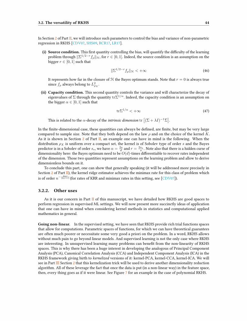
3.2. The versatility of RKHS 44
In Section 2 of Part II, we will introduce such parameters to control the bias and variance of non-parametricregression in RKHS [CDV07, SHS09, RCR17, LR17].
(i) Source condition. This rst quantity controlling the bias, will quantify the diculty of the learningproblem through ‖Σ1/2−rfρ‖H, for r ∈ [0, 1]. Indeed, the source condition is an assumption on thebigger r ∈ [0, 1] such that
‖Σ1/2−rfρ‖H < +∞ (46)
It represents how far in the closure of H the Bayes optimum stands. Note that r = 0 is always truesince fρ always belong to L2
ρX .
(ii) Capacity condition. This second quantity controls the variance and will characterize the decay ofeigenvalues of Σ through the quantity trΣ1/α. Indeed, the capacity condition is an assumption onthe bigger α ∈ [0, 1] such that
trΣ1/α < +∞ (47)
This is related to the α-decay of the intrinsic dimension tr[(Σ + λI)−1Σ
].
In the nite-dimensional case, these quantities can always be dened, are nite, but may be very largecompared to sample size. Note that they both depend on the law ρ and on the choice of the kernel K .As it is shown in Section 2 of Part II, an example one can have in mind is the following. When thedistribution ρX is uniform over a compact set, the kernel is of Sobolev type of order s and the Bayespredictor is in a Sobolev of order s∗, we have α = 2s
d and r = 2s∗s . Note also that there is a hidden curse of
dimensionality here: the Bayes optimum need to be O(d)-times dierentiable to recover rates independentof the dimension. Those two quantities represent assumptions on the learning problem and allow to derivedimensionless bounds on it.
To conclude this part, one can show that generally speaking (it will be addressed more precisely inSection 2 of Part II), the kernel ridge estimator achieves the minimax rate for this class of problem whichis of order n−
2αr2αr+1 (for rates of KRR and minimax rates in this setting, see [CDV07]).
3.2.2. Other uses
As it is our concern in Part II of this manuscript, we have detailed how RKHS are good spaces toperform regression in supervised ML settings. We will now present more succinctly ideas of applicationthat one can have in mind when considering kernel methods in statistics and computational appliedmathematics in general.
Going non-linear. In the supervised setting, we have seen that RKHS provide rich trial functions spacesthat allow for computations. Parametric spaces of functions, for which we can have theoretical guaranteesare often much poorer or necessitate some very good a priori on the problem. In a word, RKHS allowswithout much pain to go beyond linear models. And supervised learning is not the only case where RKHSare interesting. In unsupervised learning many problems can benet from the non-linearity of RKHSspaces. This is why there has been a huge interest in developing the analogous of Principal ComponentAnalysis (PCA), Canonical Correlation Analysis (CCA) and Independent Component Analysis (ICA) in theRKHS framework giving birth to kernelized versions of it: kernel-PCA, kernel-CCA, kernel-ICA. We willsee in Part III Section 2 that this kernelization trick will be used to derive another dimensionality reductionalgorithm. All of these leverage the fact that once the data is put (in a non-linear way) in the feature space,then, every thing goes as if it were linear. See Figure 7 for an example in the case of polynomial RKHS.

3.2. The versatility of RKHS 45
Figure 7 – Representation of the feature that maps in the case of order 2 polynomial RKHS in 2-d. We seethat in the feature space the data points are linearly separated. Once again, this representation is takenfrom the slides of J.-P. Vert and J. Mairal lessons on Kernel methods.
Inducing a metric. Kernels also allow to construct some metric in some a priori non-structured set X.In fact we can always dene a proper metric associated to X which is
d2K(x, x′) := ‖Kx −Kx′‖2H = K(x, x) +K(x, x)− 2K(x, x′).
This allows to compare elements in unstructured sets by comparing their associated canonical features inan Hilbert space H.
Kernelmean embedding. The theory of kernel mean embedding [SGSS07, MFSS17] cannot be summedup in such a short paragraph but let us try to explain in a few words what it is and why it can be useful. Therst thing to understand is that probability measures can be embedded in the RKHS: this is the analogousof the reproduction property for the probability measures. Indeed, one can show that
Eρ(f(X)) = 〈µρ, f〉H with µρ := Eρ[KX ].
µρ is the kernel mean embedding of the distribution ρ and for characteristic kernels, µρ encodes uniquelythe distribution ρ. This embedding allows to quantify dierences between distribution by the naturaldistance in H: this is the Maximum Mean Discrepancy (MMD) distance:
MMDH(ρ, ρ′) := sup‖f‖H61
(Eρ [f(X)]− Eρ′ [f(X)]) = ‖µρ − µρ′‖H .
This computationally tractable distance is the cornerstone of many algorithms that use measure compari-son [GBR+12].
Meshless methods and approximation theory. Finally note that kernels methods have received ahuge interest in the approximation literature for their rich, yet tractable computation properties. Anothervery interesting application in this point of view is that RKHS have the ability to reproduce derivatives offunctions and thus have been widely used in the context of PDE approximation. These are often calledadaptive or meshless methods in this literature [SW06].
?
? ?
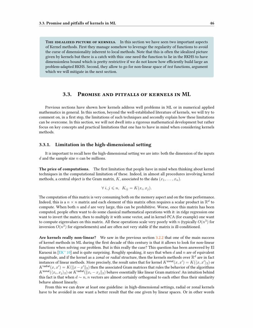
3.3. Promise and pitfalls of kernels in ML 46
The idealized picture of kernels. In this section we have seen two important aspectsof Kernel methods. First they manage somehow to leverage the regularity of functions to avoidthe curse of dimensionality inherent to local methods. Note that this is often the idealized picturegiven by kernels but there is a catch with this: one need the function to lie in the RKHS to havedimensionless bound which is pretty restrictive if we do not know how eciently build large anproblem-adapted RKHS. Second, they allow to go for non-linear space of test functions, argumentwhich we will mitigate in the next section.
3.3. Promise and pitfalls of kernels in ML
Previous sections have shown how kernels address well problems in ML or in numerical appliedmathematics in general. In this section, beyond the well-established literature of kernels, we will try tocomment on, in a rst step, the limitations of such techniques and secondly explain how these limitationscan be overcome. In this section, we will not dwell into a rigorous mathematical development but ratherfocus on key concepts and practical limitations that one has to have in mind when considering kernelsmethods.
3.3.1. Limitation in the high-dimensional setting
It is important to recall here the high-dimensional setting we are into: both the dimension of the inputsd and the sample size n can be millions.
The price of computations. The rst limitation that people have in mind when thinking about kerneltechniques in the computational limitation of these. Indeed, in almost all procedures involving kernelmethods, a central object is the Gram matrix, K , associated to the data (x1, . . . , xn).
∀ i, j 6 n, Kij = K(xi, xj).
The computation of this matrix is very consuming both on the memory aspect and on the time performance.Indeed, this is a n × n matrix and each element of this matrix often requires a scalar product in Rd tocompute. When both n and d are very large, this can be prohibitive. Worse, once this matrix has beencomputed, people often want to do some classical mathematical operations with it: in ridge regression onewant to invert the matrix, then to multiply it with some vector, and in kernel-PCA (for example) one wantto compute eigenvalues on this matrix. All these operations scale very poorly with n (typically O(n3) forinversion O(n2) for eigenelements) and are often not very stable if the matrix is ill-conditioned.
Are kernels really non-linear? We saw in the previous section 3.2.2 that one of the main successof kernel methods in ML during the rst decade of this century is that it allows to look for non-linearfunctions when solving our problem. But is this really the case? This question has been answered by ElKaraoui in [EK+10] and is quite surprising. Roughly speaking, it says that when d and n are of equivalentmagnitude, and if the kernel as a zonal or radial structure, then the kernels methods over Rd are in factinstances of linear methods. More precisely, the result sates that for kernel Kzonal(x, x′) = K(〈x, x′〉2) orKradial(x, x′) = K(‖x−x′‖2) then the associated Gram matrices that rules the behavior of the algorithmsKzonal(〈xi, xj〉2) or Kradial(‖xi−xj‖2) behave essentially like linear Gram matrices! An intuition behindthis fact is that when d ∼ n, n vectors are almost certainly orthogonal to each other thus their similaritybehave almost linearly.
From this we can draw at least one guideline: in high-dimensional settings, radial or zonal kernelshave to be avoided in one want a better result that the one given by linear spaces. Or in other words

3.3. Promise and pitfalls of kernels in ML 47
anisotropy is very important in high dimension. This is certainly one of the superiority of neural networksover (at least radial and zonal) kernels in high-dimension.
3.3.2. Choosing the right kernel
Throughout this thesis, we took the point of view of deriving bounds for general kernels leaving the roleplayed by the RKHS in modelling assumptions such that capacity and source conditions (see section 3.2.1).However, we would like to put emphasis on the fact that for real applications kernel engineering is a veryimportant task. To put this into perspective, learning the representative features of the problem all alongthe optimization path is perhaps one of the most important successes of neural networks. Playing thesame role as the architecture in neural networks, choosing the kernel has to be a problem-adapted task forthe kernel method to perform well. There are two ways to deal with such this problem:
(i) Find a priori the right kernel adapted to the problem.
(ii) Learn the kernel similarly to what happens in Neural Networks.
Problem with radial kernels. People have a tendency to think that kernel learning is a very matureeld and that in comparison to neural networks almost everything is almost known is this literature.However, I would argue that even some of the most basic and fundamental questions on kernel learningare still unsolved. Without tackling the problem of selecting a full data-driven kernel for a regressiontask, we may rst ask whether there are guidelines to tune hyper-parameters of kernels to best learn fromthe data. For example, in the simplest setting of kernel ridge regression with regularizer λ and Gaussiankernel with bandwidth σ, both λ and σ play a smoothing role but there are no precise guidelines on howto tune them to get the best accuracy. However, the role played by the bandwidth in the Gaussian kernelis huge as shows the fact that the norm of the induced space is multiplied by σd when changing the scaleof the bandwidth. To cut a long story short: learning or adapting the bandwidth of a radial kernel to theproblem seems to be an unsolved challenging theoretical and practical question.
Multiscale and hierarchical kernels. Many problems in ML have a natural multiscale structure likevision, text, signal processing, chemistry... One way to adapt to this structure can be to build a RKHSthat will take it into consideration. Those multiscale methods have shown good performances in signalprocessing and in vision with wavelets theory [Dau92] and the aim is to reproduce this in RKHS. Oneway to construct such a RKHS is to sum RKHS induced by radial kernels with dierent scales. Moreconcretely, consider φ a compactly supported function of [−1, 1] and a sequence of decreasing scalesδ1 > δ2 > . . . > δn, then we can dene Kj(x, x
′) = δ−dj φ(‖x − x′‖/δj) and j-scale approximationspaces Hj induced by Kj . Then the resulting multiscale RKHS would be:
Hmultiscale := H1 + . . .+Hn.
Another line of work concerning the will to adapt the kernel architecture to the problem has been tackledby so-called hierarchical kernels. One observation is that (isotropic) kernels often do not adapt well tothe underlying structure of the data as they treat all features as equal. This is why in [STS16], Steinwartand al. have constructed a hierarchical kernel based on composition of Gaussian kernels (activation) andweighted sums of linear kernels (layers). They also show that it was possible to nd a convex optimizationprocedure able to learn the weights of the corresponding linear kernels. Even if this line of research didnot yield yet a performance comparable to the ones of neural networks, building kernel that mimic thebehavior of neural nets with preserving kernels guarantees is very promising.
Learning the kernel. Hierarchical kernels was an attempt to nd adapted kernel to the problem. Inthis direction, let us simply mention two other attempts. The rst one is the multiple kernel learningalgorithm [BLJ04], which, in a nutshell, replaces a single kernel by a weighted sum of kernels. The

3.3. Promise and pitfalls of kernels in ML 48
advantage of this approach is that nding these weights can again be formulated as a convex objective,while the disadvantage is the limited gain in expressive power unless the used dictionary of kernels isreally huge. In the same spirit, Dutchi and al. show that it was possible to learn the best random probabilitythat lead to a random feature model [SD16].
3.3.3. Fast numerical computations
One of the major problem with kernel learning is recalled in the rst paragraph of the section: storingand computing the Gram matrix of a kernel problem can be very expensive. In this subsection, we will seehow techniques from (random) linear algebra and computer science can improve drastically the numericalperformance of such algorithms.
Subsampling and features approximations. Fortunately, to avoid the problem of calculating thewhole Gram matrix (which costs O(n2d)), we simply need low-cost approximations of the kernel ma-trix [SS02, Sec. 10.2]. More surprisingly, these approximations can improve generalization performancesas they induce a form of implicit regularization. Let us state here two important techniques related to this,for more details see Chapter 19 of [MT20].
(i) Subsampling methods. One way is to select uniformly at random p rows among the n of the kernelmatrix and perform some Nyström approximation. There exist other techniques for the rows selectionbut in practice, it is often said that uniform selection is already ecient. Note that pn ∼
√n are
necessary to recover the performance of plain kernel learning [RCR15].
(ii) Random features. Another popular way to approximate the kernel matrix is to leverage the convolu-tion structure of certain kernels [RR08]. Indeed, for convolutional kernels as in Eq. (36)
K(x, x′) :=
∫ψ(x, t)ψ(x′, t)w(t)dt,
the integral representation gives immediately a feature map ψ(x, t) to L2(w). Hence, drawing asample tj from the probability measure w(t)dt gives zj = (ψ(x1, tj), . . . , ψ(xn, tj))
> where zjz>jis an unbiased estimate of the kernel matrix K . If we repeat this procedure with r i.d.d. samples,this will give an approximation of the matrix K at Monte-Carlo rate (independent of dimension):
K ∼ Kr :=1
r
r∑j=1
zjz>j .
This procedures has only a computational cost of O(rnd), and one can obtain substantial improve-ments of performance in the case where r is small in comparison to n. Note that with this technique,we have also a direct access to the derivatives of the kernel with respect to x, x′ without additionalnumerical complexity. This will be leveraged in Part III of this thesis.
Fast numerical routines. To conclude this part, let us add that there have been huge eorts spent tospeed up the computations relative to kernel methods. The rst one is due to the work of Feydy andco-authors that developed ecient C++ routines to fasten kernel computation (of x→ Kx) of severalorder of magnitude [CFG+20]. Building on this, ecient Nyström approximations and ecient method toinvert ill-conditioned matrices, Rudi and al. developed a tool box in [MCRR20] that allow kernels to handlebillions of data points eciently. Progressed in these directions could really unlock severe limitations ofkernels and allow to re-discover techniques that were forgotten due to their slowness in the past.

3.3. Promise and pitfalls of kernels in ML 49
?
? ?
Kernel hopes and the need to dig deeper. I hope that I convinced the reader that, evenif today kernels are not as used as neural networks, there are hopes for the future of kernels thatwe manage in circumventing their natural limitations. Furthermore, let us add two characteristicsthat make them worth studying:
(i) They still give rich insights. In the recent literature there have been two examples ofkernels giving insight on ML phenomenons. First, [MM19] explains that random featurescould show a double descent behavior that has received a huge interest lately. Second, [JGH18]states that the behavior of the dynamics of neural networks is very similar to the one withan explicit kernel called the neural tangent kernel.
(ii) They give guarantees. Proving convergence guarantees for neural networks (even insimple setting) is still ongoing research. One may want solid statistical guarantees forindustrial problems, in this case neural networks could be disregarded and kernels preferred.

4. LANGEVIN DYNAMICS 50
4. Langevin Dynamics
Langevin dynamics is at the core of Part III of this thesis. This a physically anchored dynamics that isstrongly related to sampling techniques and has been “re-discovered” lately in the Machine Learningcommunity. In Section 4.1, we dene precisely what is the Langevin dynamics and how it relates to MLproblems. Then, we explain in Section 4.2 how this dynamics can be used to sample eciently distributionsin high-dimension if we manage to deal with the metastability problem described in Section 4.3. Note thatseveral paragraphs of this part are extracted from a post-doc proposal of research that I wrote to explainmy interests. As it will be clear for the reader, this part presents also my future intention of working onthe interplay between Molecular Dynamics and Machine Learning.
4.1. What is Langevin Dynamics ?
4.1.1. Denition and link with Molecular Dynamics
Langevin Dynamics. Langevin dynamics comes from statistical physics and is a system of dynamicalequations that governs the speed and positions of particles (typically atoms). To x notations, let ussuppose that N particles composed the system: typically the magnitude of N is the number of AvogadroNavo ∼ 1023, thus positions q and momenta p are both vectors of R3N . A simple, yet rich model is todivide the total energy of the microscopic system in a kinetic and a potential energy.
H(q, p) =1
2p>M−1p+ V (q),
where M is the diagonal matrix of the masses of the particles. Roughly speaking, the particles follow anHamiltonian dynamic in a thermal bath of xed temperature T with friction γ that cause uctuations oforder
√γβ−1 where β = (kBT )−1. This leads to the celebrated Langevin dynamics:
dqt = M−1ptdt
dpt = −∇V (qt)dt− γM−1ptdt+√
2γβ dWt
(48)
As discussed in [SRL10, Section 2.2.4], a simpler reversible equation can be obtained as a limit case ofLangevin dynamics by taking the large friction limit γ → +∞, small mass m→ 0 and rescaling time asγt, this gives the Overdamped Langevin dynamics:
dqt = −∇V (qt)dt+
√2
βdWt (49)
While the Langevin dynamics is a ner modelling adding some kinetic term to the equations, we willfocus on the Overdamped Langevin dynamics for simplicity, as it leads already to complex and unsolvedproblems. Note here that studying quantitatively how the add of the kinetic term in Eq.(48) changes thedynamics is an open and exciting route for future research (see subsection 4.2.2 for more details). Let ussimply mention here that one of the diculties to study the kinetic Langevin is the lack of ellipticity ofthe dynamics [Vil09] (ruled by a degenerate dissipative operator).
Molecular dynamics and sampling. MD, the computational workhorse of statistical physics, is aninterdisciplinary eld between computer science, applied mathematics and chemistry whose main objectiveis to infer macroscopic properties of matter from atomistic models via averages with respect to probabilitymeasures dictated by the principles of statistical physics [SRL10, FS01]. In a nutshell, the aim is to be ableto derive averages with respect to the canonical Boltzmann-Gibbs distribution,
µ(dq dp) = Z−1µ e−βH(q,p)dq dp, Zµ =
∫e−βH . (50)

4.1. What is Langevin Dynamics ? 51
Note that the real diculty is to sample according to q. Indeed momenta and positions are independent andthe marginal associated to the momenta follows a Gaussian distribution. The aim of molecular dynamicsis to calculate macroscopic quantities like the pressure of the system that can be express as averages withrespect to the canonical measure:
Eµ(φ) =
∫φ(q, p)µ(dq dp). (51)
What is the link with Langevin dynamics? Under certain conditions, we can show that the law ofthe processes dene by the Langevin dynamics converge to the Gibbs distribution µ(dq dp). The sameresult holds for the overdamped Langevin dynamics when considering only µ(dq) = e−V (q). Note thatfrom this point of view, the Langevin dynamics (48) and (49) are only used as sampling devices to computeaverages. Other dynamics without physical contents could be studied too, as long as they have µ(dq dp)as invariant measure!
4.1.2. Parallel MD - ML
Two motivating examples: Bayesian inference and non-convex optimization. Accurately sam-pling a certain measure π(q)dq in high dimensions is a dicult task that arises in Bayesian machinelearning. If we take V = −β−1 log π, sampling in the Bayesian framework can be directly cast into thesame problem of Molecular Dynamics.
Furthermore, note that when decreasing the temperature to 0, i.e., setting β → +∞ the Gibbs measureµ(dq) = e−β
−1V (q)dq will concentrate around the global minima of V . Hence, performing sampling atlow temperature can be a way to solve non-convex problems: this formally describes the intuition behindthe celebrated simulated annealing algorithm [VLA87].
Links between Molecular Dynamics (MD) and Machine Learning (ML). Besides sharing commongoals, let us remark that the function f to be minimized in ML and the potential V in MD share threeimportant features:
• The high-dimensionality of the underlying measure or cost-function: this is due to the numberof atoms in MD and the high-dimensionality of inputs in ML. In terms of notations, the dimension dof the inputs in ML is equal to three times the number N of particles in MD (three parameters toencode positions).
• The metastability phenomenon [Lel13] due to the multimodality of the target measure in MD,which corresponds to the non-convexity of the loss function in ML. Indeed, as we said earlier, inMD the target measure can be written µ = e−V where V can be interpreted in optimization asthe loss function to minimize, hence casting sampling problems in MD to a tempered version ofthe minimization of V . The metastability comes from the fact that the dynamics can be trappedfor long times in certain regions (modes) preventing it from ecient space exploration or ndingthe global minimum of a non-convex function. This phenomenon is often responsible for the slowconvergence of the algorithms. We will come back to this important point in section 4.3.
• In MD and ML, the question of nding low-dimensional representations (main degrees of free-dom) is crucial. Standard techniques include for example Principal Component Analysis and variants,manifold learning methods such as diusion map. Recently, ML techniques have proven to be veryuseful to perform such tasks, thanks to its ability to handle and extract the main features of highdimensional data.
?
? ?

4.2. Sampling with Langevin dynamics 52
Possible future directions and Part III’s point of view. The main point of view ofthis part of the thesis is that both elds can benet from the knowledge and know-how of theother one: MD seems to be a more mature and theoretically-anchored eld of study than ML butthe recent successes of the latter may be leveraged to solve long-standing problems of MD. Morespecically, we would like on the one hand to investigate if the sampling methods developed inMD could help to improve the learning algorithms in ML, and on the other hand to rely on recentML techniques to build reduced order models in MD.Questions. The connections highlighted above raise two symmetrical questions:
• How can techniques and principles from MD enlighten theory and practice behind MLalgorithms?
• How can the eciency of recent ML techniques help solving MD problems?
4.2. Sampling with Langevin dynamics
Besides Molecular dynamics, we have seen above that Langevin dynamics could be useful to samplethe posterior distribution in the Bayesian framework or getting near minima of non-convex functions inthe low-temperature regime. We review in this section non-asymptotic results obtained during the lastdecade, following the work of Dalalyan in [Dal17].
4.2.1. Discrete time dynamics and convergence results
Convergence of continuous time dynamics. The convergence of the continuous time dynamics is arather well-studied problem [BGL14]. Let us recall here, with usual optimization notations, the overdampedLangevin dynamics we are focused on (take β = 1 for simplicity):
dθt = −∇f(θt)dt+√
2dWt.
As (θt)t is a random process, dene its law µt. We can show that µt converges to the Gibbs distributionµ = e−f under certain conditions. Remarkably, this rate of convergence depends only on the invariantlaw µ. As in optimization with Lyapounov functions, we also need to select a convergence norm to showconvergence. One of the most common way is to show convergence in the L2(µ) metric, in this case therate of convergence is described by the Poincaré inequality [BGL14, Section 4].Denition 1 (Poincaré inequality)
We say that the probability measure dµ satises a Poincaré inequality if for all f ∈ H1(µ),
Varµ (f(X)) 6 Pµ Eµ[‖∇f(X)‖2
]. (52)
Poincaré inequalities are the cornerstone of the Part III of this thesis and we refer to longer discussions inSection 1.2.2 of this Part for details. The rate of convergence to equilibrium is encoded by the Poincaréconstant associated to µ as we have the following equivalence:
(i) µ satises a Poincaré inequality with constant Pµ;
(ii) For all f smooth and compactly supported, Varµ(Pt(f)) 6 e−2t/PµVarµ(f) for all t > 0.

4.2. Sampling with Langevin dynamics 53
Further comments are given in Section 1.2.2, but let us stress that in the case where f is ρ-strongly convex,we can show that Pµ 6 1/ρ. In a way, the Poincaré constant is the analogous of strong convexity inoptimization when it comes to sampling. Note that f need not be convex functions for µ to satisfy aPoincaré inequality.
Discrete time dynamics. First if we want to perform sampling we need to discretize the overdampedLangevin dynamics (49). As we will see, they are as much ways to perform this discretization as methodsin optimization to minimize a function. And, as in optimization, a given hypothesis on the measure tosample from will lead to an adapted discretization scheme. This is why entering into this literature canbe dicult, time-consuming and puzzling at rst sight. Hence, without seeking exhaustiveness, we willtry to focus on the main ideas behind the dierent settings. From now on, let us change the notationof the potential in Gibbs measure from V to f : µ(θ) = e−f(θ)dθ to adopt the classical notation of theoptimization literature. And keep in mind the hand-waving rule:
If a deterministic optimization algorithm performs well on a function f , then there is great chance that itsnoisy counterpart will behave almost the same to sample the probability measure e−f .
Having taken this precautions, let us write -only- the most natural discretization of (49) called explicitEuler-Maruyama :
θt+1 = θt − γ∇f(θt) +√
2γzt, (53)
where γ > 0 is the step-size and (zt)t ∼ N(0, I)N∗ is a sequence of i.i.d. Gaussian random variable in
Rd. This algorithm is often called the Unajusted Langevin Algorithm. As already said, there exist otherdiscretizations schemes, e.g. implicit Euler leads to the Proximal Langevin Algorithm and is more stable atthe cost of more expensive per-iteration complexity [Wib19].
Convergence of discrete time dynamics. As we have seen, in continuous time Poincaré inequality issucient for fast sampling as it leads to exponential convergence of the overdamped Langevin dynamics.However, in discrete time, analyzing convergence is more challenging. Indeed, to control the discretizationerror, some smoothness assumptions are required on f . Worse, the discretization error leads to anasymptotic bias: the law of the discretized dynamics converges to the wrong distribution. To correctthis bias, it is possible to apply some Metropolis lter that gives the convergence in total variationnorm [BRH13] but cannot give convergence in smoother norms as the Metropolis lter can make thedistribution singular. This is why, in an approach pioneered by Dalalyan in [Dal17], all the current analysismake step-size small enough to be as close as wanted to the Gibbs measure µ. This said, there exist asmuch results as possible settings: convergence in dierent probability norms, for dierent discretizationsand under dierent assumptions (some weaker, some stronger than Poincaré inequality). For example,typical number of steps to be ε-close to the Gibbs distribution is of order O(P2
µd3/2ε−1) in the case of a
Poincaré inequality assumption [Wib19].
4.2.2. What can we do with MD knowledge ?
Analysis of stochastic algorithms. One of the main dierence between MD and ML preventing fromdirect knowledge transfer is that the main foci of the two disciplines are dierent. Indeed, in MD, people areinterested in sampling according to a given target measure, whereas in ML, the focus in on the minimizationof some objective function. Note that those two questions coincide in the zero temperature limit. Hence, itseems possible to transfer technical tools to analyze algorithms in computational statistical physics to tryto improve non-asymptotic bounds for Langevin-type discretizations algorithms which are often the mainfocus of ML works [RRT17, DM19].

4.3. The metastability problem 54
Accelerating the dynamics. More importantly, one active eld of study in MD and ML is to try toaccelerate the stochastic dynamics at hand. These techniques rely on changing it without aectingthe invariant measure while accelerating the convergence to equilibrium. We could (i) study Kineticversions of Langevin dynamics [MCC+19], (ii) add some drift term or (iii) some non-reversibility throughbirth-and-death processes [LLN19].
?
? ?
Understanding continuous-time SGD. The Langevin dynamics seems very related tostochastic gradient descent with additive noise as we have seen in Section 2 of this introduction.In this same direction, while the ML community has solid knowledge of discrete-time dynamics,understanding continuous versions of the algorithms often leads to a deeper comprehension of thebehavior of the systems. Such a paradigm is often used in MD where mathematical tools weredesigned to tackle such problems. This could lead to the study of the continuous counterpart ofthe stochastic gradient descent algorithm [LT19]. Knowing how the noise and potentials behavein SGD will be the key to apply the ideas from MD and the study the possible metastability of thedynamics.
4.3. The metastability problem
4.3.1. What is metastability ?
The metastability problem of Langevin dynamics comes from the two scales involved in the physicalproblem. Indeed, particles behave very dierently at the microscopic level and at a macroscopic one whereinteresting properties emerge from collective behavior. This discrepancy between those two scales isrelated to the fact that the system remains trapped for long time in restricted regions of the space ofconguration. And it may take a large characteristic time to “jump” into another metastable state. In factat a coarse grained level, people have modeled the behavior of the particle system by a jump process atcertain rate from one region to another [Lel13].
Computationally-wise, metastability is an important problem because it prevents from ecient spaceexploration and implies that the convergence to the stationary distribution can be very slow. One caneasily picture two wells separated by some barrier such that it is a rare event to see the particle going froma well to another one. This is a well-known evidence of metastability (arising because of non-convexity)and large deviation theory [FW98] showed that the typical time scale to go from one well to the othergrows exponentially with the inverse of temperature. This is what we call an energetic barrier and isrepresented in Figure 8 (a-b). Another type of metastability can occur: entropic barriers are due to the factthat the path to go from one region of conguration space to the other may be hard to ne. This is thecase with the tiny corridor represented in Figure 8 (c-d).
A quantitative measure of metastability: Poincaré inequality. A natural question then is how toquantify the metastability of the process. Metastability summarizes qualitatively the fact that the dynamicis very slow due to non-convex eect of the landscape or narrow transitions between separated regionsof space. We have seen that the Poincaré constant is itself a measure of non-convexity of the potentialand we can show that it degrades also linearly with temperature in the presence of entropic barriers.

4.3. The metastability problem 55
Figure 8 – (a,c) Level sets of the two-dimensional potentials in the cases of (a) energetic barrier (c) entropicbarrier. (b, d) Evolution along the x-axis of the overdamped Langevin diusion in these potentials. Thisgure is extracted from [LS16].
Actually, Poincaré constant or other quantication of convergence (logarithmic Sobolev inequality are theone detailed in [Lel13]) are very well suited to quantify such a phenomenon. Throughout this thesis andespecially in Part III, we will keep in mind the following idea:
The larger the Poincaré constant, the more metastable the process is.
Note here that the dependence in the number of step as the square of the Poincaré constant in the discretetime analysis of Langevin dynamics can make the estimation of the invariant measure computationallyintractable as soon as it is too big.
4.3.2. Avoiding metastability
Reaction coordinates. Obtaining a good collective variable (i.e. reduced models with fewer degrees offreedom) is a crucial problem in computational statistical physics. It allows to grasp physical behaviorsof the systems at a coarse-grained level. This low-dimensional representation, a.k.a. reaction coordinates,should index properly transitions between the modes of the probability measure and is the cornerstone inMD to tackle the issue of metastability and accelerate the dynamics.
To illustrate this, let us consider the two examples described in Figure 8. In the two examples, (b) and(d) show cases where the particle stay during long times in restricted regions of the space: in (b) x ∼ ±1and in (d) x ∼ ±2. Hence, in both cases, there are two metastable states and the transition between thetwo states can be described by the x-coordinate. This x-coordinate is thus a slow variable of the systemcompared to the y-coordinate and typical time of changes are much longer than the classical diusion inthe metastable region.
More generally speaking a reaction coordinate is a function
ξ : Rd → Rp, p 6 d. (54)
such that (ξ(qt))t is a metastable process. ξ should encode the transition path between the metastablestates. Coming from molecular chemistry, we can understand this denomination as it represents the

4.3. The metastability problem 56
coordinate (or path) is congurational space along which chemical reactions occur. It is a reduced ordermodel, hence, the smaller the p the more practical and intuitive the reaction coordinate is. In examplescoming from MD, it could be the angle of a protein characterizing the conformation of a molecule, or theposition of a material defect.
Finding a good Reaction Coordinate (RC) is of great important both for chemists and computer scientistsof the domain. However, today, practitioners need some a priori knowledge or deep physical intuitionon the system to nd RC. One of the aim of the Part III of this manuscript is to automatically nd goodRC during the sampling procedure leveraging statistical methods. In this context, we proposed in Part III,Section 2 a general algorithm to nd reaction coordinates by estimating the spectral gap of the overdampedLangevin dynamics for a given target probability, using samples of this measure.
Using reaction coordinates to accelerate the dynamics. Reaction coordinates are very useful forchemists to understand better the properties of the system. In the eyes of computer scientists, RC areused to accelerate the dynamics by applying free energy biasing methods such that the free energy biaseddynamics reaches equilibrium much faster than the original unbiased dynamics [LRS08]. The process isvery well described in [LS16, Section 4] and we will only sketch the main principle here. Note also thatthese techniques have also been studied in the high-dimensional Bayesian framework to accelerate thesampling dynamics in the case of a Gaussian mixture model [CLS12].
Circumventing the diculty caused by metastability by leveraging the knowledge of reaction coordinaterests upon two ideas:
(i) Using importance sampling strategies by changing the original potential V to V − F (ξ(·)) whereF is the free energy associated with the RC ξ. Roughly speaking, F is the potential associated withµF := ξ#µ the image of the measure µ by ξ.
(ii) Since µF = ξ#µ, F is not available in practice. The second idea is to use a current estimate Ft thatwill be better and better along the dynamics. This adaptive feature explains why method of thistype are called free energy adaptive biasing techniques.
The intuition behind the idea of changing the potential with the free energy is that by doing so, themetastable features of the original potential along ξ will be removed. Indeed, we can show that along ξthe biased measure with potential V − F (ξ(·)) is uniform: this allows for fast sampling!
?? ?
Conclusion of the introduction. Throughout this introduction we have tried to showhow naturally what were the main questions of this thesis. Here are the main messages to takehome. In the rst section 1, we tried to put a particular emphasis on the fact that optimization wasabsolutely unavoidable in the high-dimensional ML setting. Going further in Section 2, we tried toconvince the reader that stochastic versions of classical rst order methods are the cornerstoneof these optimization techniques by the low-cost but also their ability to give good estimators.After this, we took a detour in Section 3 to the non-parametric world of RKHS demonstrating thatthere were still many unsolved questions in this eld that may lead them to properly competewith neural networks. We nally show in Section 4 that analyzing high-dimensional algorithmsthrough the lens of their continuous-time counterpart could enlighten their properties, allow tofocus on MD-related question such as metastability and accelerate them.I have now introduced my personal way of thinking in ML and my personal questions, interestsand foci. I hope it will enlighten the reading of what consists in the core of this thesis: Part II andIII.

This is a fucking blank sentence.
57
Part II
Non-parametric
Stochastic Gradient descent
We divide this part into our two contributions for non-parametric Stochastic gradient descent.
The Section 1 together with its Appendix A shows the exponential convergence of Stochastic gradientdescent of the binary test loss in the case where the classication is easy: we talk about a hard margincondition. Side results in this work could be of their own interest: among them are derived high probabilitybounds in ‖ · ‖∞ norm for non-parametric SGD resting on concentration and fast rates under low-noiseconditions à la Mammen and Tsybakov are derived. This section is based on our work, Exponentialconvergence of testing error for stochastic gradient methods, L. Pillaud-Vivien, A. Rudi and F. Bach,published in the Conference On Learning Theory in 2018.
The Section 2 and its Appendix B are focus on optimality of SGD in the non-parametric setting. Moreprecisely, this work is the rst to show that multiple passes over the data allow to reach optimality in certaincases where the Bayes optimum is hard to approximate. This work tries to reconcile theory and practiceas common knowledge on SGD always stated that one pass over the data is optimal. This section is basedon our work, Statistical Optimality of Stochastic Gradient Descent on Hard Learning Problems
through Multiple Passes, L. Pillaud-Vivien, A. Rudi and F. Bach, published in the Advances in NeuralInformation Processing Systems in 2018.
58

Contents
1 Exponential convergence of testing error for stochastic gradient methods 60
1.1 Introduction . . . . . . . . . . . . . . . . . . . . . . . . . . . . . . . . . . . . . . . . . . . 601.2 Problem Set-up . . . . . . . . . . . . . . . . . . . . . . . . . . . . . . . . . . . . . . . . . 611.3 Concrete Examples and Related Work . . . . . . . . . . . . . . . . . . . . . . . . . . . . . 631.4 Stochastic Gradient descent . . . . . . . . . . . . . . . . . . . . . . . . . . . . . . . . . . . 641.5 Exponentially Convergent SGD for Classication error . . . . . . . . . . . . . . . . . . . 681.6 Conclusion . . . . . . . . . . . . . . . . . . . . . . . . . . . . . . . . . . . . . . . . . . . . 69
A Appendix of Exponential convergence of testing error for stochastic gra-
dient descent 71
A.1 Experiments . . . . . . . . . . . . . . . . . . . . . . . . . . . . . . . . . . . . . . . . . . . 71A.2 Probabilistic lemmas . . . . . . . . . . . . . . . . . . . . . . . . . . . . . . . . . . . . . . 73A.3 From H to 0-1 loss . . . . . . . . . . . . . . . . . . . . . . . . . . . . . . . . . . . . . . . . 74A.4 Exponential rates for Kernel Ridge Regression . . . . . . . . . . . . . . . . . . . . . . . . 75A.5 Proofs and additional results about concrete examples . . . . . . . . . . . . . . . . . . . . 77A.6 Preliminaries for Stochastic Gradient Descent . . . . . . . . . . . . . . . . . . . . . . . . 80A.7 Proof of stochastic gradient descent results . . . . . . . . . . . . . . . . . . . . . . . . . . 81A.8 Exponentially convergent SGD for classication error . . . . . . . . . . . . . . . . . . . . 91A.9 Extension of Corollary 1 and Theorem 4 for the full averaged case. . . . . . . . . . . . . . 93A.10 Convergence rate under weaker margin assumption . . . . . . . . . . . . . . . . . . . . . 97
2 Statistical Optimality of SGD on Hard Learning Problems through Mul-
tiple Passes 100
2.1 Introduction . . . . . . . . . . . . . . . . . . . . . . . . . . . . . . . . . . . . . . . . . . . 1002.2 Least-squares regression in nite dimension . . . . . . . . . . . . . . . . . . . . . . . . . 1012.3 Averaged SGD with multiple passes . . . . . . . . . . . . . . . . . . . . . . . . . . . . . . 1032.4 Application to kernel methods . . . . . . . . . . . . . . . . . . . . . . . . . . . . . . . . . 1042.5 Experiments . . . . . . . . . . . . . . . . . . . . . . . . . . . . . . . . . . . . . . . . . . . 1062.6 Conclusion . . . . . . . . . . . . . . . . . . . . . . . . . . . . . . . . . . . . . . . . . . . . 108
B Appendix of Statistical Optimality of SGD on Hard Learning Problems
through Multiple Passes 110
B.1 A general result for the SGD variance term . . . . . . . . . . . . . . . . . . . . . . . . . . 110B.2 Proof sketch for Theorem 8 . . . . . . . . . . . . . . . . . . . . . . . . . . . . . . . . . . . 114B.3 Bounding the deviation between SGD and batch gradient descent . . . . . . . . . . . . . 115B.4 Convergence of batch gradient descent . . . . . . . . . . . . . . . . . . . . . . . . . . . . 117B.5 Experiments with dierent sampling . . . . . . . . . . . . . . . . . . . . . . . . . . . . . 128
59

1. Exponential convergence of testing
error for stochastic gradient meth-
ods
1.1. Introduction
Stochastic gradient methods are now ubiquitous in machine learning, both from the practical side,as a simple algorithm that can learn from a single or a few passes over the data [BLC05], and from thetheoretical side, as it leads to optimal rates for estimation problems in a variety of situations [NY83, PJ92].
They follow a simple principle [RM51]: to nd a minimizer of a function F dened on a vector spacefrom noisy gradients, simply follow the negative stochastic gradient and the algorithm will converge to astationary point, local minimum or global minimum of F (depending on the properties of the functionF ), with a rate of convergence that decays with the number of gradient steps n typically as O(1/
√n),
or O(1/n) depending on the assumptions which are made on the problem [PJ92, NV08, NJLS09, SSSS07,Xia10, BM11, BM13, DFB17].
On the one hand, these rates are optimal for the estimation of the minimizer of a function given accessto noisy gradients [NY83], which is essentially the usual machine learning set-up where the function F isthe expected loss, e.g., logistic or hinge for classication, or least-squares for regression, and the noisygradients are obtained from sampling a single pair of observations.
On the other hand, although these rates as O(1/√n) or O(1/n) are optimal, there are a variety of
extra assumptions that allow for faster rates, even exponential rates.First, for stochastic gradient from a nite pool, that is for F = 1
k
∑ki=1 Fi, a sequence of works starting
from SAG [RSB12], SVRG [JZ13], SAGA [DBLJ14], have shown explicit exponential convergence. However,these results, once applied to machine learning where the function Fi is the loss function associated withthe i-th observation of a nite training data set of size k, say nothing about the loss on unseen data (testloss). The rates we present in this paper are on unseen data.
Second, assuming that at the optimum all stochastic gradients are equal to zero, then for strongly-convex problems (e.g., linear predictions with low-correlated features), linear convergence rates can beobtained for test losses [Sol98, SL13]. However, for supervised machine learning, this has limited relevanceas having zero gradients for all stochastic gradients at the optimum essentially implies prediction problemswith no uncertainty (that is, the output is a deterministic function of the input). Moreover, we can only getan exponential rate for strongly-convex problems and thus this imposes a parametric noiseless problem,which limits the applicability (even if the problem was noiseless, this can only reasonably be in a non-parametric way with neural networks or positive denite kernels). Our rates are on noisy problems andon innite-dimensional problems where we can hope that we approach the optimal prediction functionwith large numbers of observations. For prediction functions described by a reproducing kernel Hilbertspace, and for the square loss, the excess testing loss (equal to testing loss minus the minimal testing lossover all measurable prediction functions) is known to converge to zero at a subexponential rate typicallygreater than O(1/n) [DB16, DFB17], these rates being optimal for the estimation of testing losses.
Going back to the origins of supervised machine learning with binary labels, we will not considergetting to the optimal testing loss (using a convex surrogate such as logistic, hinge or least-squares) butthe testing error (number of mistakes in predictions), also referred to as the 0-1 loss.
It is known that the excess testing error (testing error minus the minimal testing error over allmeasurable prediction functions) is upper bounded by a function of the excess testing loss [Zha04, BJM06],but always with a loss in the convergence rate (e.g., no dierence or taking square roots). Thus a slow ratein O(1/n) or O(1/
√n) on the excess loss leads to a slow(er) rate on the excess testing error.
Such general relationships between excess loss and excess error have been rened with the use ofmargin conditions, which characterize how hard the prediction problems are [MT99]. Simplest input points
60

1.2. Problem Set-up 61
are points where the label is deterministic (i.e., conditional probabilities of the label are equal to zeroor one), while hardest points are the ones where the conditional probabilities are equal to 1/2. Marginconditions quantify the mass of input points which are hardest to predict, and lead to improved transferfunctions from testing losses to testing errors, but still no exponential convergence rates [BJM06].
In this paper, we consider the strongest margin condition, that is conditional probabilities are boundedaway from 1/2, but not necessarily equal to 0 or 1. This assumption on the learning problem has been usedin the past to show that regularized empirical (convex) risk minimization leads to exponential convergencerates [AT07, KB05]. Our main contribution is to show that stochastic gradient descent also achievessimilar rates (see an empirical illustration in Figure 10 in the Appendix A.1). This requires several sidecontributions that are interesting on their own, that is, a new and simple formalization of the learningproblem that allows exponential rates of estimation (regardless of the algorithms used to nd the estimator)and a new concentration result for averaged stochastic gradient descent (SGD) applied to least-squares,which is ner than existing work [BM13].
The paper is organized as follows: in Section 1.2, we present the learning set-up, namely binaryclassication with positive denite kernels, with a particular focus on the relationship between errors andlosses. Our main results rely on a generic condition for which we give concrete examples in Section 1.3. InSection 1.4, we present our version of stochastic gradient descent, with the use of tail averaging [JKK+16],and provide new deviation inequalities, which we apply in Section 1.5 to our learning problem, leadingto exponential convergence rates for the testing errors. We conclude in Section 1.6 by providing severalavenues for future work. Finally, synthetic experiments illustrating our results can be found in Section A.1of the Appendix.
Main contributions of the paper. We would like to underline that our main contributions are in the twofollowing results; (a) we show in Theorem 4 the exponential convergence of stochastic gradient descent onthe testing error, and (b) this result strongly rests on a new deviation inequality stated in Corollary 1 forstochastic gradient descent for least-squares problems. This last result is interesting on its own and givesan improved high-probability result which does not depend on the dimension of the problem and has atighter dependence on the strongly convex parameter –through the eective dimension of the problem,see [CDV07, DB16].
1.2. Problem Set-up
In this section, we present the general machine learning set-up, from generic assumptions to morespecic assumptions.
1.2.1. Generic assumptions
We consider a measurable set X and a probability distribution ρ on data (x, y) ∈ X × −1, 1; wedenote by ρX the marginal probability on x, and by ρ(±1|x) the conditional probability that y = ±1 givenx. We have E(y|x) = ρ(1|x)− ρ(−1|x). Our main margin condition is the following (and independent ofthe learning framework):
(A1) |E(y|x)| > δ almost surely for some δ ∈ (0, 1].
This margin condition (often referred to as a low-noise condition) is commonly used in the theoretical studyof binary classication [MT99, AT07, KB05], and usually takes the following form: ∀δ > 0, P(|E(y|x)| <δ) = O(δα) for α > 0. Here, however, δ is a xed constant. Our stronger margin condition (A1) isnecessary to show exponential convergence rates but we give also explicit rates in the case of the latterlow-noise condition. This extension is derived in Appendix A.10 and more precisely in Corollary 4. Notethat the smaller the α, the larger the mass of inputs with hard-to-predict labels. Our condition corresponds
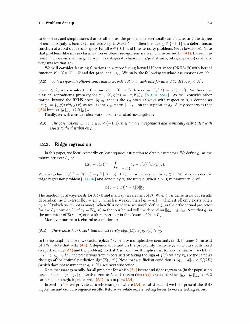
1.2. Problem Set-up 62
to α = +∞, and simply states that for all inputs, the problem is never totally ambiguous, and the degreeof non-ambiguity is bounded from below by δ. When δ = 1, then the label y ∈ −1, 1 is a deterministicfunction of x, but our results apply for all δ ∈ (0, 1] and thus to noisy problems (with low noise). Notethat problems like image classication or object recognition are well characterized by (A1). Indeed, thenoise in classifying an image between two disparate classes (cars/pedestrians, bikes/airplanes) is usuallyway smaller that 1/2.
We will consider learning functions in a reproducing kernel Hilbert space (RKHS) H with kernelfunction K : X× X→ R and dot-product 〈·, ·〉H. We make the following standard assumptions on H:
(A2) H is a separable Hilbert space and there exists R > 0, such that for all x ∈ X,K(x, x) 6 R2.
For x ∈ X, we consider the function Kx : X → R dened as Kx(x′) = K(x, x′). We have theclassical reproducing property for g ∈ H, g(x) = 〈g,Kx〉H [STC04, SS02]. We will consider othernorms, beyond the RKHS norm ‖g‖H, that is the L2-norm (always with respect to ρX), dened as‖g‖2L2
=∫Xg(x)2dρX(x), as well as the L∞-norm ‖ · ‖L∞ on the support of ρX. A key property is that
(A2) implies ‖g‖L∞ 6 R‖g‖H.Finally, we will consider observations with standard assumptions:
(A3) The observations (xn, yn) ∈ X× −1, 1, n ∈ N∗ are independent and identically distributed withrespect to the distribution ρ.
1.2.2. Ridge regression
In this paper, we focus primarily on least-squares estimation to obtain estimators. We dene g∗ as theminimizer over L2 of
E(y − g(x))2 =
∫X×−1,1
(y − g(x))2dρ(x, y).
We always have g∗(x) = E(y|x) = ρ(1|x)− ρ(−1|x), but we do not require g∗ ∈ H. We also consider theridge regression problem [CDV07] and denote by gλ the unique (when λ > 0) minimizer in H of
E(y − g(x))2 + λ‖g‖2H.
The function gλ always exists for λ > 0 and is always an element of H. When H is dense in L2 our resultsdepend on the L∞-error ‖gλ − g∗‖∞, which is weaker than ‖gλ − g∗‖H which itself only exists wheng∗ ∈ H (which we do not assume). When H is not dense we simply dene g∗ as the orthonormal projectorfor the L2 norm on H of g∗ = E(y|x) so that our bound will the depend on ‖gλ − g∗‖∞. Note that g∗ isthe minimizer of E(y − g(x))2 with respect to g in the closure of H in L2.
Moreover our main technical assumption is:
(A4) There exists λ > 0 such that almost surely, sign(E(y|x))gλ(x) >δ
2.
In the assumption above, we could replace δ/2 by any multiplicative constants in (0, 1) times δ (insteadof 1/2). Note that with (A4), λ depends on δ and on the probability measure ρ, which are both xed(respectively by (A1) and the problem), so that λ is xed too. It implies that for any estimator g such that‖gλ − g‖L∞ < δ/2, the predictions from g (obtained by taking the sign of g(x) for any x), are the same asthe sign of the optimal prediction sign(E(y|x)). Note that a sucient condition is ‖gλ − g‖H < δ/(2R)(which does not assume that g∗ ∈ H), see next subsection.
Note that more generally, for all problems for which (A1) is true and ridge regression (in the populationcase) is so that ‖gλ−g∗‖L∞ tends to zero as λ tends to zero then (A4) is satised, since ‖gλ−g∗‖L∞ 6 δ/2for λ small enough, together with (A1) then implies (A4).
In Section 1.3, we provide concrete examples where (A4) is satised and we then present the SGDalgorithm and our convergence results. Before we relate excess testing losses to excess testing errors.

1.3. Concrete Examples and Related Work 63
1.2.3. From testing losses to testing error
Here we provide some results that will be useful to prove exponential rates for classication withsquared loss and stochastic gradient descent. First we dene the 0-1 loss dening the classication error:
R(g) = ρ((x, y) : sign(g(x)) 6= y),
where signu = +1 for u ≥ 0 and −1 for u < 0. In particular denote by R∗ the so-called Bayes riskR∗ = R(E[y|x]) which is the minimum achievable classication error [DGL13].
A well known approach to bound the testing errors by testing losses is via transfer functions. Inparticular we recall the following result [DGL13, BJM06], let g∗(x) be equal to E[y|x] a.e., then
R(g)− R∗ ≤ φ(‖g − g∗‖2L2), ∀g ∈ L2(dρX),
with φ(u) =√u (or φ(u) = uβ , with β ∈ [1/2, 1], depending on some properties of ρ [BJM06]. While
this result does not require (A1) or (A4), it does not readily lead to exponential rates since the squaredloss excess risk has minimax lower bounds that are polynomial in n [CDV07].
Here we follow a dierent approach, requiring via (A4) the existence of gλ having the same sign as g∗and with absolute value uniformly bounded from below. Then we can bound the 0-1 error with respect tothe distance in H of the estimator g from gλ as shown in the next lemma (proof in Appendix A.3). Thiswill lead to exponential rates when the distribution satises a margin condition (A1) as we prove in thenext section and in Section 1.5. Note also that for the sake of completeness we recalled in Appendix A.4that exponential rates could be achieved for kernel ridge regression.Lemma 1 (From approximately correct sign to 0-1 error)
Let q ∈ (0, 1). Under (A1), (A2), (A4), g ∈ H a random function such that ‖g − gλ‖H < δ2R , with
probability at least 1− q. Then
R(g) = R∗, with probability at least 1− q, and in particular ER(g)− R∗ ≤ q.
In the next section we provide sucient conditions and explicit settings naturally satisfying (A4).
1.3. Concrete Examples and Related Work
In this section we illustrate specic settings that naturally satisfy (A4). We start by the followingsimple result showing that the existence of g∗ ∈ H such that g∗(x) = E[y|x] a.e. on the support of ρX, issucient to have (A4) (proof in Appendix A.5.1).Proposition 3
Under (A1), assume that there exists g∗ ∈ H such that g∗(x) := E[y|x] on the support of ρX, then for
any δ, there exists λ > 0 satisfying (A4), that is, sign(E(y|x))gλ(x) >δ
2.
We are going to use the proposition above to derive more specic settings. In particular we considerthe case where the positive and negative classes are separated by a margin that is strictly positive. LetX ⊆ Rd and denote by S the support of the probability ρX and by S+ = x ∈ X : g∗(x) > 0 thepart associated to the positive class, and by S− the one associated with the negative class. Consider thefollowing assumption:
(A5) There exists µ > 0 such that minx∈S+,x′∈S− ‖x− x′‖ ≥ µ.
Denote by W s,2 the Sobolev space of order s dened with respect to the L2 norm, on Rd (see [AF03] andAppendix A.5.2). We also introduce the following assumption:

1.4. Stochastic Gradient descent 64
(A6) X ⊆ Rd and the kernel is such thatW s,2 ⊆ H, with s > d/2.
An example of kernel such that H = W s,2, with s > d/2 is the Abel kernel K(x, x′) = e−1σ ‖x−x
′‖, forσ > 0. In the following proposition we show that if there exist two functions in H, one matching E[y|x]on S+ and the second matching E[y|x] on S− and if the kernel satises (A6), then (A4) is satised.Proposition 4
Under (A1), (A5), (A6), if there exist two functions g∗+, g∗− ∈ W s,2 such that g∗+(x) = E[y|x] on S+
and g∗−(x) = E[y|x] on S−, then (A4) is satised.
Finally we are able to introduce another setting where (A4) is naturally satised (the proof of the propositionabove and the example below are given in Appendix A.5.2).Example 1 (Independent noise on the labels)
Let ρX be a probability distribution on X ⊆ Rd and let S+, S− ⊆ X be a partition of the support of ρXsatisfying ρX(S+), ρX(S−) > 0 and (A5). Let n ∈ N∗. For 1 ≤ i ≤ n, xi independently sampled fromρX and the label yi dened by the law
yi =
ζi if xi ∈ S+
−ζi if xi ∈ S−,
with ζi independently distributed as ζi = −1 with probability p ∈ [0, 1/2) and ζi = 1 with probability1− p. Then (A1) is satised with δ = 1− 2p and (A4) is satised as soon as (A2) and (A6) are, that is,the kernel is bounded and H is rich enough (see an example in Appendix A.5 Figure 12).
Finally note that the results of this section can be easily generalized from X = Rd to any Polish space,by using a separating kernel [DVRT14, RCDVR14] instead of (A6).
1.4. Stochastic Gradient descent
We now consider the stochastic gradient algorithm to solve the ridge regression problem with axed strictly positive regularization parameter λ. We consider solving the regularized problem withregularization ‖g− g0‖2H through stochastic approximation starting from a function g0 ∈ H (typically 0).1Denote by F : H→ R, the functional
F (g) = E(Y − g(X))2 = E(Y − 〈KX , g〉)2,
where the last identity is due to the reproducing property of the RKHS H. Note that F has the followinggradient ∇F (g) = −2E [(Y − 〈KX , g〉)KX ]. We consider also Fλ = F + λ‖ · −g0‖2H, for which∇Fλ(g) = ∇F (g) + 2λ(g − g0), and we have for each pair of observation (xn, yn) that Fλ(g) =E[Fn,λ(g)
]= E(〈g,Kxn〉 − yn)2 + λ‖g − g0‖2H, with Fn,λ(g) = (〈g,Kxn〉 − yn)2 + λ‖g − g0‖2H.
Denoting Σ = E[Kxn ⊗Kxn
]the covariance operator dened as a linear operator from H to H (see
[FBJ04] and references therein), we have the optimality conditions for gλ and g∗:
Σgλ − E (ynKxn) + λ(gλ − g0) = 0, E [(yn − g∗(xn))Kxn ] = 0,
see [CDV07] or Appendix A.6.1 for the proof of the last identity. Let (γn)n>1 be a positive sequence; weconsider the stochastic gradient recursion2 in H started at g0:
gn = gn−1 −γn2∇Fn,λ(gn−1) = gn−1 − γn [(〈Kxn , gn−1〉 − yn)Kxn + λ(gn−1 − g0)] . (55)
1Note that g0 is the initialization of the recursion, and is not the limit of gλ when λ tends to zero (this limit being g∗).2The complexity of n steps of the recursion is O(n2) if using kernel functions or O(τn) when using explicit feature representa-
tions, with τ the complexity of computing dot-products and adding feature vectors.

1.4. Stochastic Gradient descent 65
We are going to consider Polyak-Ruppert averaging [PJ92], that is gn = 1n+1
∑ni=0 gi, as well as the
tail-averaging estimate gtailn = 1
bn/2c∑ni=bn/2c gi, studied by [JKK+16]. For the sake of clarity, all the
results in the main text are for the tail averaged estimate but note that all of them have been also provedfor the full average in Appendix A.9.
As explained earlier (see Lemma 1), we need to show the convergence of gn to gλ in H-norm. We aregoing to consider two cases: (1) for the non-averaged recursion (γn) is a decreasing sequence, with theimportant particular case γn = γ/nα, for α ∈ [0, 1]; (2) for the averaged or tail-averaged functions (γn) isa constant sequence equal to γ. For all the proofs of this section see Appendix A.7. In the next subsectionwe reformulate the recursion in Eq. (55) as a least-squares recursion converging to gλ.
1.4.1. Reformulation as noisy recursion
We can rst reformulate the SGD recursion equation in Eq. (55) as a regular least-squares SGD recursionwith noise, with the notation ξn = yn − g∗(xn), which satises E
[ξnKxn
]= 0. This is the object of the
following lemma (for the proof see Appendix A.6.2.):Lemma 2
The SGD recursion can be rewritten as follows:
gn − gλ =[I − γn(Kxn ⊗Kxn + λI)
](gn−1 − gλ) + γnεn, (56)
with the noise term εk = ξkKxk + (g∗(xk)− gλ(xk))Kxk − E [(g∗(xk)− gλ(xk))Kxk ] ∈ H.
We are thus in presence of a least-squares problem in the Hilbert space H, to estimate a function gλ ∈ H
with a specic noise εn in the gradient and feature vector Kx. In the next section, we will considerthe generic recursion above, which will require some bounds on the noise. In our setting, we have thefollowing almost sure bounds and the noise (see Lemma 9 of Appendix A.7):
‖εn‖H 6 R(1 + 2‖g∗ − gλ‖L∞)
E[εn ⊗ εn
]4 2
(1 + ‖g∗ − gλ‖2∞
)Σ,
where Σ = E[Kxn ⊗Kxn
]is the covariance operator.
1.4.2. SGD for general Least-Square problems
We now consider results on (averaged) SGD for least-squares that are interesting on their own. Assaid before, we show results in two dierent settings depending on the step-size sequence. First, weconsider (γn) as a decreasing sequence, second we take (γn) constant but prove the convergence of the(tail-)averaged iterates.
Since the results we need could be of interest (even for nite-dimensional models), in this section, westudy the following general recursion:
ηn = (I − γHn)ηn−1 + γnεn, (57)
We make the following assumptions:
(H1) We start at some η0 ∈ H.
(H2) (Hn, εn)n>1 are i.i.d. andHn is a positive self-adjoint operator so that almost surelyHn < λI , andH := EHn.
(H3) Noise: Eεn = 0, ‖εn‖H 6 c1/2 almost surely and E(εn ⊗ εn) 4 C , with C commuting with H .Note that one consequence of this assumption is E‖εn‖2H 6 trC .

1.4. Stochastic Gradient descent 66
(H4) For all n > 1, E[HnCH
−1Hn
]4 γ−1
0 C and γ 6 γ0.
(H5) A is a positive self-adjoint operator which commutes with H .
Note that we will later apply the results of this section to Hn = Kxn ⊗Kxn + λI , H = Σ + λI , C = Σand A ∈ I,Σ. We rst consider the non-averaged SGD recursion, then the (tail-)averaged recursion.The key dierence with existing bounds is the need for precise probabilistic deviation results.
For least-squares, one can always separate the impact of the initial condition η0 and of the noiseterms εk , namely ηn = ηbias
n + ηvariancen , where ηbias
n is the recursion with no noise (εk = 0), and ηvariancen is
the recursion started at η0 = 0. The nal performance will be bounded by the sum of the two separateperformances (see, e.g.,[DB15]). Hence all of our bounds will depend on these two. See more details inAppendix A.7.
1.4.3. Non-averaged SGD
In this section, we prove results for the recursion dened by Eq. (57) in the case where for α ∈ [0, 1],γn = γ/nα. These results extend the ones of [BM11] by providing deviation inequalities, but are limitedto least-squares. For general loss functions and in the strongly-convex case, see also [KT09].Theorem 1 (SGD, decreasing step size: γn = γ/nα)
Assume (H1), (H2), (H3), γn = γ/nα, γλ < 1 and denote by ηn ∈ H the n-th iterate of the recursionin Eq. (57). We have for t > 0, n > 1 and α ∈ (0, 1),
‖gn − gλ‖H 6 exp
(− γλ
1− α((n+ 1)1−α − 1
))‖g0 − gλ‖H + Vn,
almost surely for n large enough 3, with P (Vn > t) 6 2 exp
(− t2
8γtrC/λ+ γc1/2t· nα
).
We can make the following observations:
• The proof technique (see Appendix A.7.1 for the detailed proof) relies on the following scheme: wenotice that ηn can be decomposed in two terms, (a) the bias: obtained from a product of n contractantoperators, and (b) the variance: a sum of increments of a martingale. We treat separately the twoterms. For the second one, we prove almost sure bounds on the increments and on the variance thatlead to a Bernstein-type concentration result on the tail P(Vn > t). Following this proof technique,the coecient in the latter exponential is composed of the variance bound plus the almost surebound of the increments of martingale times t.
• Note that we only presented in Theorem 1 the case where α ∈ (0, 1). Indeed, we only focused on thecase where we had exponential convergence (see the whole result in the Appendix: Proposition 8).Actually, that there are three dierent regimes. For α = 0 (constant step-size), the algorithm is notconverging, as the tail probability bound on P (Vn > t) is not dependent on n. For α = 1, conrmingresults from [BM11], there is no exponential forgetting of initial conditions. And for α ∈ (0, 1),the forgetting of initial conditions and the tail probability are converging to zero exponentiallyfast, respectively, as exp(−Cn1−α) and exp(−Cnα), for a constant C , hence the natural choice ofα = 1/2 in our experiments.
1.4.4. Averaged and Tail-averaged SGD with constant step-size
In the subsection, we take: ∀n > 1, γn = γ. We rst start with a result on the variance term, whoseproof extends the work of [DFB17] to deviation inequalities which are sharper than the ones from [BM13].

1.4. Stochastic Gradient descent 67
Theorem 2 (Convergence of the variance term in averaged SGD)
Assume (H1), (H2), (H3), (H4), (H5) and consider the average of the n+ 1 rst iterates of the sequencedened in Eq. (57): ηn = 1
n+1
∑ni=0 ηi. Assume η0 = 0. We have for t > 0, n > 1:
P(∥∥∥A1/2ηn
∥∥∥H
> t)6 2 exp
[− (n+ 1)t2
Et
], (58)
where Et is dened with respect to the constants introduced in the assumptions:
Et = 4tr(AH−2C) +2c1/2‖A1/2‖op
3λ· t. (59)
The work that remains to be done is to bound the bias term of the recursion ηbiasn . We have done it
for the full averaged sequence (see Appendix A.9.1 Theorem 6) but as it is quite technical and couldlower a bit the clarity of the reasoning, we have decided to leave it in the Appendix. We present hereanother approach and consider the tail-averaged recursion, ηtail
n = 1bn/2c
∑ni=bn/2c ηi (as proposed by
[JKK+16, Sha11]). For this, we use the simple almost sure bound ‖ηbiasi ‖H 6 (1− λγ)i‖η0‖H, such that
‖ηtail, biasn ‖H 6 (1− λγ)n/2‖η0‖H. For the variance term, we can simply use the result above for n and
n/2, as ηtailn = 2ηn − ηn/2. This leads to:
Corollary 1 (Convergence of tail-averaged SGD)
Assume (H1), (H2), (H3), (H4), (H5) and consider the tail-average of the sequence dened in Eq. (57):ηtailn = 1
bn/2c∑ni=bn/2c ηi. We have for t > 0, n > 1:∥∥∥A1/2ηtailn
∥∥∥H
6 (1− γλ)n/2‖A1/2‖op‖η0‖H + Ln , with (60)
P(Ln > t) 6 4 exp(−(n+ 1)t2/(4Et)
), (61)
where Ln is dened in the proof (see Appendix A.7.3) and is the variance term of the tail-averaged recur-sion.
We can make the following observations on the two previous results:
• The proof technique (see Appendix A.7.2 and A.7.3 for the detailed proofs) relies on concentrationinequality of Bernstein type. Indeed, we notice that (in the setting of Theorem 2) ηn is a sum ofincrements of a martingale. We prove almost sure bounds on the increments and on the variance(following the proof technique of [DFB17]) that lead to a Bernstein type concentration result on thetail P(Vn > t). Following the proof technique summed-up before, we see that Et is composed ofthe variance bound plus the almost sure bound times t.
• Remark that classically, A and C are proportional to H for excess risk predictions. In the nited-dimensional setting this leads us to the usual variance bound proportional to the dimension d:tr(AH−2C) ∼= trI = d. The result is general in the sense that we can apply it for all matrices Acommuting with H (this can be used to prove results in L2 or in H).
• Finally, note that we improved the variance bound with respect to the strong convexity parameterλ which is usually of the order 1/λ2 (see [Sha11]), and is here tr(AH−2C). Indeed, in our setting,we will apply it for A = C = Σ and H = Σ + λI , so that tr(AH−2C) is upper bounded by theeective dimension tr(Σ(Σ + λI)−1) which can be way smaller than 1/λ2 (see [CDV07, DB16]).
• The complete proof for the full average is written in Appendix A.9.1 and more precisely in Theorem6. In this case the initial conditions are not forgotten exponentially fast though.

1.5. Exponentially Convergent SGD for Classication error 68
1.5. Exponentially Convergent SGD for Classification
error
In this section we want to show our main results, on the error made (on unseen data) by the n-thiterate of the regularized SGD algorithm. Hence, we go back to the original SGD recursion dened inEq. (56). Let us recall it:
gn − gλ =[I − γn(Kxn ⊗Kxn + λI)
](gn−1 − gλ) + γnεn,
with the noise term εk = ξkKxk + (g∗(xk)− gλ(xk))Kxk − E [(g∗(xk)− gλ(xk))Kxk ] ∈ H. Like in theprevious section we are going to state two results in two dierent settings, the rst one for SGD withdecreasing step-size (γn = γ/nα) and the second one for tail averaged SGD with constant step-size. Forall the proofs of this section see the Appendix (section A.8).
1.5.1. SGD with decreasing step-size
In this section, we focus on decreasing step-sizes γn = γ/nα for α ∈ (0, 1), which lead to exponentialconvergence rates. Results for α = 1 and α = 0 can be derived in a similar way (but do not lead toexponential rates).Theorem 3
Assume (A1), (A2), (A3), (A4) and γn = γ/nα, α ∈ (0, 1) for any n and γλ < 1. Let gn be then-th iterate of the recursion dened in Eq. (56), as soon as n satises exp
(− γλ
1−α((n+ 1)1−α − 1
))6
δ/(5R‖g0 − gλ‖H), then
R(gn) = R∗, with probability at least 1− 2 exp
(− δ2
CR· nα
),
with CR = 2α+7γR2trΣ(1 + ‖g∗ − gλ‖2∞
)/λ+ 8γR2δ(1 + 2‖g∗ − gλ‖∞)/3, and in particular
ER(gn)− R∗ 6 2 exp
(− δ2
CR· nα
).
Note that Theorem 3 shows that with probability at least 1− 2 exp(− δ2
CR· nα
), the predictions of gn are
perfect. We can also make the following observations:
• The idea of the proof (see Appendix A.8.1 for the detailed proof) is the following: we know that assoon as ‖gn − gλ‖H 6 δ/(2R), the predictions of gn are perfect (Lemma 1). We just have to applyTheorem 1 for to the original SGD recursion and make sure to bound each term by δ/(4R). Similarresults for non-averaged SGD could be derived beyond least-squares (e.g., hinge or logistic loss)using results from [KT09].
• Also note that the larger the α, the smaller the bound. However, it is only valid for n larger that acertain quantity depending of λγ. A good trade-o is α = 1/2, for which we get an excess errorof 2 exp
(− δ2
CRn1/2
), which is valid as soon as n > log(10R‖g0 − gλ‖H/δ)/(4λ2γ2). Notice also
that we should go for large γλ to increase the factor in the exponential and make the conditionhappen as soon as possible.
• If we want to emphasize the dependence of the bound on the important parameters, we can writethat: ER(gn)− R∗ . 2 exp
(−λδ2nα/R2
).

1.6. Conclusion 69
• When the condition on n is not met, then we still have the usual bound obtained by taking directlythe excess loss [BJM06] but we lose exponential convergence.
1.5.2. Tail averaged SGD with constant step-size
We now consider the tail-averaged recursion4, with the following result:Theorem 4
Assume (A1), (A2), (A3), (A4) and γn = γ for any n, γλ < 1 and γ 6 γ0 = (R2 + 2λ)−1. Letgn be the n-th iterate of the recursion dened in Eq. (56), and gtailn = 1
bn/2c∑ni=bn/2c gi, as soon as
n > 2/(γλ) ln(5R‖g0 − gλ‖H/δ), then
R(gtailn ) = R∗, with probability at least 1− 4 exp(−δ2KR(n+ 1)
),
with K−1R = 29R2
(1 + ‖g∗ − gλ‖2∞
)tr(Σ(Σ + λI)−2) + 32δR2(1 + 2‖g∗ − gλ‖∞)/(3λ), and in
particularER(gtailn )− R∗ 6 4 exp
(−δ2KR(n+ 1)
).
Theorem 4 shows that with probability at least 1 − 4 exp(−δ2KR(n+ 1)
), the predictions of gtail
n areperfect. We can also make the following observations:
• The idea of the proof (see Appendix A.8.2 for the detailed proof) is the following: we know thatas soon as ‖gtail
n − gλ‖H 6 δ/(2R), the predictions of gtailn are perfect (Lemma 1). We just have to
apply Corollary 1 to the original SGD recursion, and make sure to bound each term by δ/(4R).
• If we want to emphasize the dependence of the bound on the important parameters, we can writethat: ER(gn)− R∗ . 2 exp
(−λ2δ2n/R4
). Note that the λ2 could be made much smaller with
assumptions on the decrease of eigenvalues of Σ (it has been shown [CDV07] that if the decayhappens at speed 1/nβ : trΣ(Σ + λI)−2 6 λ−1trΣ(Σ + λI)−1 6 R2/λ1+1/β).
• We want to take γλ as big as possible to satisfy quickly the condition. In comparison to theconvergence rate in the case of decreasing step-sizes, the dependence on n is improved as theconvergence is really an exponential of n (and not of some power of n as in the previous result).
• Finally, the complete proof for the full average is contained in Appendix A.9.2 and more precisely inTheorem 7.
1.6. Conclusion
In this paper, we have shown that stochastic gradient could be exponentially convergent, once somemargin conditions are assumed; and even if a weaker margin condition is assumed, fast rates can beachieved (see Appendix A.10). This is obtained by running averaged stochastic gradient on a least-squaresproblem, and proving new deviation inequalities.
Our work could be extended in several natural ways: (a) our work relies on new concentration resultsfor the least-mean-squares algorithm (i.e., SGD for square loss), it is natural to extend it to other losses,such as the logistic or hinge loss; (b) going beyond binary classication is also natural with the squareloss [CRR16, OBLJ17] or without [TCKG05]; (c) in our experiments, we use regularization, but we haveexperimented with unregularized recursions, which do exhibit fast convergence, but for which proofs
4The full averaging result corresponding to Theorem 4 is proved in Appendix A.9.2, Theorem 7.

1.6. Conclusion 70
are usually harder [DB16]; nally, (d) in order to avoid the O(n2) complexity, extending the resultsof [RCR17, RR17] would lead to a subquadratic complexity.
?
? ?

A. AppendixofExponential convergence
of testing error for stochastic gra-
dient descent
A.1. Experimentswhere the experiments and their settings are explained.
A.2. Probabilistic lemmaswhere concentration inequalities in Hilbert spaces used in section A.7 are recalled.
A.3. FromH to 0-1 losswhere, from high probability bound for ‖ · ‖H, we derived bound for the 0-1 error.
A.4. Proofs of Exponential rates for Kernel Ridge Regressionwhere exponential rates for Kernel Ridge Regression are proven (Theorem 5).
A.5. Proofs and additional results about concrete exampleswhere additional results and croncrete examples to satisfy (A4) are given.
A.6. Preliminaries for Stochastic Gradient Descentwhere the SGD recursion is derived.
A.7. Proof of stochastic gradient descent resultswhere high probability bounds for the general SGD recursion are shown (Theorems 1 and 2).
A.8. Exponentially convergent SGD for classication errorwhere exponential convergence of test error are shown (Theorems 3 and 4).
A.9. Extension for the full averaged casewhere previous results are extended for full averaged SGD (instead of tail-averaged).
A.10. Convergence under weaker margin assumptionwhere previous results are extended in the case of a weaker margin assumption.
A.1. Experiments
To illustrate our results, we consider one-dimensional synthetic examples (X = [0, 1]) for which ourassumptions are easily satised. Indeed, we consider the following set-up that fulls our assumptions:
• (A1), (A3) We consider here X ∼ U ([0, (1− ε)/2] ∪ [(1 + ε)/2, 1]) and with the notations ofExample 1, we take S+ = [0, (1− ε)/2] and S− = [(1 + ε)/2, 1]. For 1 ≤ i ≤ n, xi independentlysampled from ρX we dene yi = 1 if xi ∈ S+ and yi = −1 if xi ∈ S−.
• (A2) We take the kernel to be the exponential kernel K(x, x′) = exp(−|x − x′|) for which theRKHS is a Sobolev space H = W s,2, with s > d/2, which is dense in L2 [AF03].
• (A4) With this setting we could nd a closed form for gλ and checked that it veried (A4). Indeedwe could solve the optimality equation satised by gλ :
∀z ∈ [0, 1],
∫ 1
0
K(x, z)gλ(x)dρX(x) + λgλ(z) =
∫ 1
0
K(x, z)gρ(x)dρX(x),
71

A.1. Experiments 72
the solution being a linear combination of exponentials in each set : [0, (1−ε)/2], [(1−ε)/2, (1+ε)/2]and [(1 + ε)/2, 1].
0.0 0.2 0.4 0.6 0.8 1.0
−1.0
−0.5
0.0
0.5
1.0
1.5
ǫ
gλ
ρX
[y|x]
Figure 9 – Representing the ρX density (uniform with ε-margin), the best estimator, i.e., E(x|y) and gλused for the simulations (λ = 0.01).
In the case of SGD with decreasing step size, we computed only the test error E(R(gn)− R∗)). Fortail averaged SGD with constant step size, we computed the test error as well as the training error, the testloss (which corresponds to the L2 loss :
∫ 1
0(gn(x)− gλ(x))2dρ(x)) and the training loss. In all cases we
computed the errors of the n-th iterate with respect to the calculated gλ, taking g0 = 0. For any n > 1,
gn = gn−1 − γn[(gn−1(xn)− yn)Kxn + λgn−1
].
We can use representants to nd the recursion on the coecients. Indeed, if gn =∑ni=1 a
ni Kxi , then
the following recursion for the (ani ) reads :
for i 6 n− 1, ani = (1− γnλ)an−1i
ann = −γn(
n−1∑i=1
an−1i K(xn, xi)− yn).
From (ani ), we can also compute the coecients of gn and gtailn that we note ani and an,tail
i respectively:ani =
∑nk=i
akin+1 and an,tail
i = 1bn/2c
∑nk=bn/2c a
ki . To show our theoretical results we have decided to
present the following gures:
• For the exponential convergence of the averaged and tail averaged cases, we plotted the errorlog10 E(R(gn)− R∗)) as a function of n. With this scale and following our results it goes as a lineafter a certain n (Figures 10 and 11 right).
• We recover the results of [DFB17] that show convergence at speed 1/n for the loss (Figure 10 left).We adapted the scale to compare with the error plot.
• For Figure 11 left, we plotted − log(− log(E(R(gn)− R∗))) of the excess error with respect to thelog of n to show a line of slope −1/2. It meets our theoretical bound of the form exp(−K
√n),
Note that for the plots where we plotted the expected excess errors, i.e., E(R(gn)− R∗), we plottedthe mean of the errors over 1000 replications until n = 200, whereas for the plots where we plotted thelosses, i.e., a function of ‖gn − g∗‖2, we plotted the mean of the loss over 100 replications until n = 2000.
We can make the following observations:First remark that between plots of losses and errors (Figure 10 left and right resp.), there is a factor 10
between the numbers of samples (200 for errors and 2000 for losses) and another factor 10 between errors
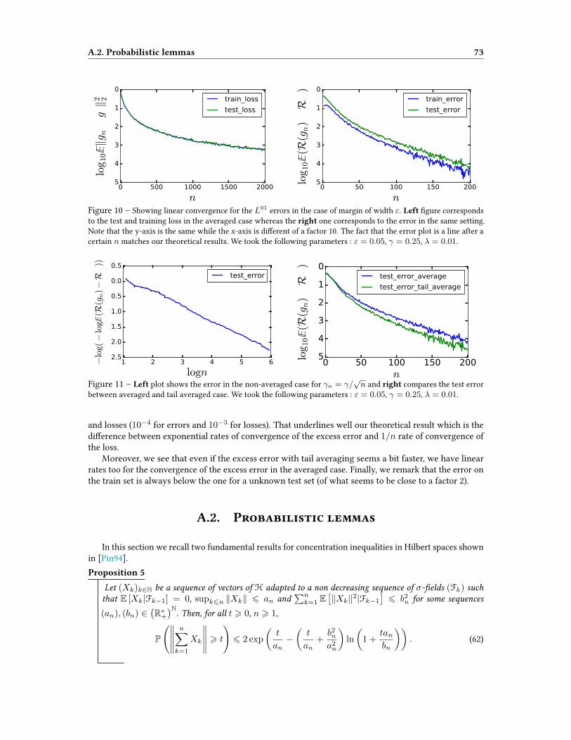
A.2. Probabilistic lemmas 73
0 500 1000 1500 2000
n
−5
−4
−3
−2
−1
0
log10‖g
n−g λ‖2 2 train_loss
test_loss
0 50 100 150 200
n
−5
−4
−3
−2
−1
0
log10(R
(gn)−R
∗ ) train_error
test_error
Figure 10 – Showing linear convergence for the L01 errors in the case of margin of width ε. Left gure correspondsto the test and training loss in the averaged case whereas the right one corresponds to the error in the same setting.Note that the y-axis is the same while the x-axis is dierent of a factor 10. The fact that the error plot is a line after acertain n matches our theoretical results. We took the following parameters : ε = 0.05, γ = 0.25, λ = 0.01.
1 2 3 4 5 6
logn
−2.5
−2.0
−1.5
−1.0
−0.5
0.0
0.5
−log
(−
log
(R(g
n)−R
∗ ))
test_error
0 50 100 150 200n
−5
−4
−3
−2
−1
0
log10(R
(gn)−R
∗ )
test_error_average
test_error_tail_average
Figure 11 – Left plot shows the error in the non-averaged case for γn = γ/√n and right compares the test error
between averaged and tail averaged case. We took the following parameters : ε = 0.05, γ = 0.25, λ = 0.01.
and losses (10−4 for errors and 10−3 for losses). That underlines well our theoretical result which is thedierence between exponential rates of convergence of the excess error and 1/n rate of convergence ofthe loss.
Moreover, we see that even if the excess error with tail averaging seems a bit faster, we have linearrates too for the convergence of the excess error in the averaged case. Finally, we remark that the error onthe train set is always below the one for a unknown test set (of what seems to be close to a factor 2).
A.2. Probabilistic lemmas
In this section we recall two fundamental results for concentration inequalities in Hilbert spaces shownin [Pin94].Proposition 5
Let (Xk)k∈N be a sequence of vectors of H adapted to a non decreasing sequence of σ-elds (Fk) suchthat E [Xk|Fk−1] = 0, supk6n ‖Xk‖ 6 an and
∑nk=1 E
[‖Xk‖2|Fk−1
]6 b2n for some sequences
(an), (bn) ∈(R∗+)N
. Then, for all t > 0, n > 1,
P
(∥∥∥∥∥n∑k=1
Xk
∥∥∥∥∥ > t
)6 2 exp
(t
an−(t
an+b2na2n
)ln
(1 +
tanbn
)). (62)

A.3. From H to 0-1 loss 74
Proof : As E [Xk|Fk−1] = 0, the Fj-adapted sequence (fj) dened by fj =∑jk=1 Xk is a martingale and so is
the stopped-martingale (fj∧n). By applying Theorem 3.4 of [Pin94] to the martingale (fj∧n), we have theresult.
Corollary 2
Let (Xk)k∈N be a sequence of vectors of H adapted to a non decreasing sequence of σ-elds (Fk) suchthat E [Xk|Fk−1] = 0, supk6n ‖Xk‖ 6 an and
∑nk=1 E
[‖Xk‖2|Fk−1
]6 b2n for some sequences
(an), (bn) ∈(R∗+)N
. Then, for all t > 0, n > 1,
P
(∥∥∥∥∥n∑k=1
Xk
∥∥∥∥∥ > t
)6 2 exp
(− t2
2 (b2n + ant/3)
). (63)
Proof : We apply 5 and simply notice that
t
an−(t
an+b2na2n
)ln
(1 +
tanbn
)= − b
2n
a2n
((1 +
ant
b2n
)ln
(1 +
ant
b2n
)− ant
b2n
)= − b
2n
a2n
φ
(ant
b2n
),
where φ(u) = (1 + u) ln(1 + u)− u for u > 0. Moreover φ(u) >u2
2 (1 + u/3), so that:
t
an−(t
an+b2na2n
)ln
(1 +
tanbn
)6 − b
2n
a2n
(ant/b2n)2
2 (1 + ant/3b2n)= − t2
2 (b2n + ant/3).
A.3. From H to 0-1 loss
In this section we prove Lemma 1. Note that (A4) requires the existence of gλ having the same sign ofg∗ almost everywhere on the support of ρX and with absolute value uniformly bounded from below. InLemma 1 we prove that we can bound the 0-1 error with respect to the distance in H of the estimator gform gλ.Proof of Lemma 1 : Denote by W the event such that
∥∥g − gλ∥∥H < δ/(2R). Note that for any f ∈ H,
f(x) = 〈f,Kx〉H ≤∥∥Kx
∥∥H
∥∥f∥∥H≤ R
∥∥f∥∥H,
for any x ∈ X. So for g ∈W , we have
|g(x)− gλ(x)| ≤ R∥∥g − gλ∥∥H < δ/2 ∀x ∈ X.
Let x be in the support of ρX. By (A4) |gλ(x)| ≥ δ/2 a.e.. Let g ∈ W and x ∈ X such that gλ(x) > 0,we have
g(x) = gλ(x)− (gλ(x)− g(x)) ≥ gλ(x)− |gλ(x)− g(x)| > 0,
so sign(g(x)) = sign(gλ(x)) = +1. Similarly let g ∈W and x ∈ X such that gλ(x) < 0, we have
g(x) = gλ(x) + (g(x)− gλ(x)) ≤ gλ(x) + |gλ(x)− g(x)| < 0,
so sign(g(x)) = sign(gλ(x)) = −1. Finally note that for any g ∈ H, by (A4), either gλ(x) > 0 or gλ(x) < 0a.e., so sign(g(x)) = sign(gλ(x)) a.e.
Now note that by (A1), (A4) we have that sign(g∗(x)) = sign(gλ(x)) a.e., where g∗(x) := E[y|x]. Sowhen g ∈W , we have that sign(g(x)) = sign(gλ(x)) = sign(g∗(x)) a.e., so
R(g) = ρ((x, y) : sign(g(x)) 6= y) = ρ((x, y) : sign(g∗(x)) 6= y) = R∗.

A.4. Exponential rates for Kernel Ridge Regression 75
Finally note thatER(g) = ER(g)1W + ER(g)1Wc ,
where 1W is 1 on the set W and 0 outside, W c is the complement set of W . So, when g ∈W , we have
ER(g)1W = R∗E1W ≤ R
∗,
whileER(g)1Wc ≤ E1Wc ≤ q.
A.4. Exponential rates for Kernel Ridge Regression
A.4.1. Results
In this section, we rst specialize some results already known in literature about the consistencyof kernel ridge least-squares regression (KRLS) in H-norm [CDV07] and then we derive exponentialclassication learning rates. Let (xi, yi)
ni=1 be n examples independently and identically distributed
according to ρ, that is Assumption (A3). Denote by Σ, Σ the linear operators on H dened by
Σ =1
n
n∑i=1
Kxi ⊗Kxi , Σ =
∫X
(Kx ⊗Kx)dρX(x),
referred to as the covariance and empirical (non-centered) covariance operators (see [FBJ04] and referencestherein). We recall that the KRLS estimator gλ ∈ H, which minimizes the regularized empirical risk, isdened as follows in terms of Σ,
gλ = (Σ + λI)−1
(1
n
n∑i=1
yiKxi
).
Moreover we recall that the population regularized estimator gλ is characterized by see ([CDV07])
gλ = (Σ + λI)−1 (EyKx) .
The following lemma bounds the empirical regularized estimator with respect to the population one interms of λ, n and is essentially contained in the work of [CDV07]; here we rederive it in a subcase (seebelow for the proof).Lemma 3
Under assumption (A2), (A3) for any λ > 0, note un = ‖ 1n
∑ni=1 yiKxi − EyKx‖H and vn =
‖Σ− Σ‖op, we have:
‖gλ − gλ‖H ≤unλ
+Rvnλ2
.
By using deviation inequalities for un, vn in Lemma 3 and then applying Lemma 1, we obtain the followingexponential bound for kernel ridge regression (see complete proof below):Theorem 5
Under (A1), (A2), (A3), (A4) we have that for any n ∈ N,
R(gλ)− R∗ = 0 with probability at least 1− 4 exp
(−C0λ
4δ2
R8n
).
Moreover, ER(gλ)− R∗ ≤ 4 exp(−C0λ
4δ2n/R8), with C−1
0 := 72(1 + λR2)2.

A.4. Exponential rates for Kernel Ridge Regression 76
The result above is a renement of Thm. 2.6 from [YRC07]. We improved the dependency in n andremoved the requirements that g∗ ∈ H or g∗ = Σrw for a w ∈ L2(dρX) and r > 1/2. Similar resultsexist for losses that are usually considered more suitable for classication, like the hinge or logistic lossand more generally losses that are non-decreasing [KB05]. With respect to this latter work, our analysisuses the explicit characterization of the kernel ridge regression estimator in terms of linear operators on H
[CDV07]. This, together with (A4), allows us to use analytic tools specic to reproducing kernel Hilbertspaces, leading to proofs that are comparatively simpler, with explicit constants and a clearer problemsetting (consisting essentially in (A1), (A4) and no assumptions on E[y|x]).
Finally note that the exponent of λ could be reduced by using a rened analysis under additionalregularity assumption of ρX and E[y|x] (as source condition and intrinsic dimension from [CDV07]), but itis beyond the scope of this paper.
A.4.2. Proofs
Here we prove that Kernel Ridge Regression achieves exponential classication rates under assump-tions (A1), (A4). In particular by Lemma 3 we bound
∥∥gλ − gλ∥∥H in high probability and then we useLemma 1 that gives exponential classcation rates when
∥∥gλ − gλ∥∥H is small enough in high probability.Proof of Lemma 3 : Denote by Σλ the operator Σ + λI and with Σλ the operator Σ + λI . We have
gλ − gλ = Σ−1λ
(1
n
n∑i=1
yiKxi
)− Σ−1
λ (EyKx)
= Σ−1λ
(1
n
n∑i=1
yiKxi − EyKx
)+ (Σ−1
λ − Σ−1λ )EyKx.
For the rst term, since∥∥Σ−1
λ
∥∥op ≤ λ
−1, we have
∥∥Σ−1λ
(1
n
n∑i=1
yiKxi − EyKx
)∥∥H≤∥∥Σ−1
λ
∥∥op
∥∥ 1
n
n∑i=1
yiKxi − EyKx
∥∥H
≤ 1
λ
∥∥ 1
n
n∑i=1
yiKxi − EyKx
∥∥H.
For the second term, since ‖Σ−1λ ‖op ≤ λ−1 and ‖EyKx‖ ≤ E‖yKx‖ ≤ R, we have∥∥(Σ−1
λ − Σ−1λ )EyKx
∥∥H
=∥∥Σ−1
λ (Σ− Σ)Σ−1λ EyKx
∥∥H
≤∥∥Σ−1
λ
∥∥op
∥∥Σ− Σ∥∥
op
∥∥Σ−1λ
∥∥op
∥∥EyKx
∥∥H≤ R
λ2
∥∥Σ− Σ∥∥
op.
Proof of Theorem 5 : Let τ > 0. By Lemma 2 we know that
‖gλ − gλ‖H ≤unλ
+Rvnλ2
,
with un = ‖ 1n
∑ni=1(yiKxi − EyKx)‖H and vn = ‖Σ − Σ‖op. For un we can apply Pinelis inequality
(Thm. 3.5, [Pin94]), since (xi, yi)ni=1 are sampled independently according to the probability ρ and that
yiKxi − EyKx is zero mean. Since ∥∥ 1
n(yiKxi − EyKx)
∥∥H≤ 2R
n
a.e. and H is a Hilbert space, then we apply Pinelis inequality with b2∗ = 4R2
nand D = 1, obtaining
un ≤√
8R2τ
n,

A.5. Proofs and additional results about concrete examples 77
with probability at least 1− 2e−τ . Now, denote by∥∥·∥∥
HSthe Hilbert-Schmidt norm and recall that
∥∥·∥∥ ≤∥∥·∥∥HS
. To bound vn we apply again the Pinelis inequality [RBV10] considering that the space of Hilbert-Schmidt operators is again a Hilbert space and that Σ = 1
n
∑ni=1 Kxi ⊗Kxi , that (xi)
ni=1 are independently
sampled from ρX and that EKxi ⊗Kxi = Σ. In particular we apply it with D = 1 and b2∗ = 4R4
n, so
vn =∥∥Σ− Σ
∥∥ ≤ ∥∥Σ− Σ∥∥HS≤√
8R4τ
n,
with probability 1−2e−τ . Finally we take the intersection bound of the two events obtaining, with probabilityat least 1− 4e−τ ,
‖gλ − gλ‖H ≤√
8R2τ
λ2n+
√8R6τ
λ4n.
By selecting τ = δ2
9R2(
√8R2
λ2n+
√8R6
λ4n)2
, we obtain ‖gλ − gλ‖H ≤ δ3R
, with probability 1 − 4e−τ . Now we
can apply Lemma 1 to have the exponential bound for the classication error.
A.5. Proofs and additional results about concrete
examples
In the next subsection we prove that g∗ ∈ H is sucient to satisfy (A4), while in subsection A.5.2 weprove that specic settings naturally satisfy (A4).
A.5.1. From g∗ ∈ H to (A4)
Here we assume that there exists g∗ ∈ H such that g∗(x) = E[y|x] a.e. on the support of ρX. Firstwe introduce A(λ), that is a quantity related to the approximation error of gλ with respect to g∗ and westudy its behavior when λ→ 0. Then we express
∥∥gλ − g∗∥∥H in terms of A(λ). Finally we prove that forany δ given by (A1), there exists λ such that (A4) is satised.
Let (σt, ut)t∈N be an eigenbasis of Σ with σ1 ≥ σ2 ≥ · · · ≥ 0, and let αj = 〈g∗, uj〉 we introduce thefollowing quantity
A(λ) =∑t:σt≤λ
α2t .
Lemma 4
Under (A2), A(λ) is decreasing for any λ > 0 and
limλ→0
A(λ) = 0.
Proof : Under (A2) and the linearity of trace, we have that∑j∈N
σj = tr(Σ) =
∫tr (Kx ⊗Kx) dρX(x) =
∫〈Kx,Kx〉H dρX(x) =
∫K(x, x)dρX(x) ≤ R2.
Denote by tλ ∈ N, the number mint ∈ N | σt ≤ λ. Since the (σj)j∈N is a non-decreasing summablesequence, then it converges to 0, then
limλ→0
tλ =∞.
Finally, since (α2j )j∈N is a summable sequence we have that
limλ→0
A(λ) = limλ→0
∑t:σt≤λ
α2t = lim
λ→0
∑j=tλ
α2j = lim
t→∞
∞∑j=t
α2j = 0.

A.5. Proofs and additional results about concrete examples 78
Here we express∥∥gλ − g∗∥∥H in terms of
∥∥g∗∥∥H and of A(√λ).
Lemma 5
Under (A2), for any λ > 0 we have∥∥gλ − g∗∥∥H ≤√√λ∥∥g∗∥∥2
H+A(
√λ).
Proof : Denote by Σλ the operator Σ + λI . Note that since g∗ ∈ H, then
EyKx = Eg∗(x)Kx = E(Kx ⊗Kx)g∗ = EKx ⊗Kxg∗ = Σg∗,
then gλ = Σ−1λ EyKx = Σ−1
λ Σg∗. So we have∥∥gλ − g∗∥∥H =∥∥Σ−1
λ Σg∗ − g∗∥∥H
=∥∥(Σ−1
λ Σ− I)g∗∥∥H
= λ∥∥Σ−1
λ g∗∥∥H.
Moreover
λ∥∥(Σ + λI)−1g∗
∥∥H≤√λ∥∥(Σ + λI)−1/2
∥∥√λ∥∥(Σ + λI)−1/2g∗∥∥H≤√λ∥∥(Σ + λI)−1/2g∗
∥∥H.
Now we express√λ∥∥(Σ + λI)−1/2g∗
∥∥H
in terms of A(λ). We have that
λ∥∥(Σ + λI)−1/2g∗
∥∥2
H= λ
⟨g∗, (Σ + λI)−1g∗
⟩= λ
⟨g∗,
∑j∈N
(σj + λ)−1uj ⊗ uj
g∗
⟩
=∑j∈N
λα2j
σj + λ.
Now divide the series in two parts∑j∈N
λα2j
σj + λ= S1(λ) + S2(λ), S1(λ) =
∑j:σj≥
√λ
λα2j
σj + λ, S2(λ) =
∑j:σj<
√λ
λα2j
σj + λ.
For each term in S1, since j is selected such that σj ≥√λ we have that λ(σj + λ)−1 ≤ λ(
√λ+ λ)−1 ≤
λ/√λ ≤√λ, so
S1(λ) ≤√λ
∑j:σj≥
√λ
α2j ≤√λ∑j∈N
α2j =√λ∥∥g∗∥∥2
.
For S2, we have that λ(σj + λ)−1 ≤ 1, so
S2(λ) ≤∑
j:σj<√λ
α2j = A(
√λ).
Proof of Proposition 3 : By Lemma 5 we have that∥∥gλ − g∗∥∥H ≤√√λ∥∥g∗∥∥2
H+A(
√λ).
Now note that the r.h.s. is non-decreasing in λ, and is 0 when λ→ 0, due to Lemma 4. Then there exists λsuch that
∥∥gλ − g∗∥∥H < δ2R
.Since |f(x)| ≤ R
∥∥f∥∥H
for any f ∈ H when the kernel satises (A2) and moreover (A1) holds, we havethat for any x ∈ X such that g∗(x) > 0 we have
gλ(x) = g∗(x)− (g∗(x)− gλ(x)) ≥ g∗(x)− |g∗(x)− gλ(x)| ≥ δ −R∥∥gλ − g∗∥∥ ≥ δ/2,
so sign(g∗(x)) = sign(gλ(x)) = +1 and sign(g∗(x))gλ(x) ≥ δ/2. Analogously for any x ∈ X such thatg∗(x) < 0 we have
gλ(x) = g∗(x) + (gλ(x)− g∗(x)) ≤ g∗(x) + |g∗(x)− gλ(x)| ≤ −δ +R∥∥gλ − g∗∥∥ ≤ −δ/2,
so sign(g∗(x)) = sign(gλ(x)) = −1 and sign(g∗(x))gλ(x) ≥ δ/2. Note nally that g∗(x) = 0 on a zeromeasure set by (A4).

A.5. Proofs and additional results about concrete examples 79
A.5.2. Examples
In this subsection we rst introduce some notation and basic results about Sobolev spaces, then weprove Prop. 4 and Example 1.
In what follows denote by At the t-fattening of a set A ⊆ Rd, that is At =⋃x∈P Bt(x) where Bt(x)
is the open ball of ray t centered in x. We denote by W s,2(Rd) the Sobolev space endowed with norm
∥∥f∥∥W s,2 =
f ∈ L1(Rd) ∩ L2(Rd)
∣∣∣∣ ∫Rd
F(f)(ω)2(1 + ‖ω‖2)s/2dω <∞.
Finally we dene the function φs,t : X→ R, that will be used in the proofs as follows
φs,t(x) = qd,δ t−d 10t(x) (1− ‖x/t‖2)s−d/2,
with qd,s = π−d/2Γ(1 + s)/Γ(1 + s− d/2) and t > 0, s ≥ d/2. Note that φs,t(x) is supported on 0ε/2,satises ∫
Rdφs,t(y)dy = 1
and it is continuous and belongs to W s,2(Rd).Proposition 6
Let P,N two compact subsets of Rd with Hausdor distance at least ε > 0. There exists gP,N ∈ W s,2
such thatgP,N (x) = 1, ∀ x ∈ P, qP,N (x) = 0, ∀ x ∈ N.
In particular gP,N = 1Pε/2 ∗ φs,ε/2.
Proof : Denote by vε,s the function (1− ‖2x/ε‖2)s−d/2. We have
gP,N (x) = qd,s(ε/2)−d∫Rd
1Pε/2(x− y) 10ε/2(y) vε,s(y) dy
= qd,s(ε/2)−d∫0ε/2
1Pε/2(x− y) vε,s(y) dy
= qd,s(ε/2)−d∫xε/2
1Pε/2(y) vε,s(y − x) dy
Now when x ∈ P , then xε/2 ⊆ Pε/2, so
gP,N (x) = qd,s(ε/2)−d∫xε/2
1Pε/2(y) vε,s(y − x) dy
= qd,s(ε/2)−d∫xε/2
vε,s(y − x)dy = qd,sε−d∫0ε/2
vε,s(y)dy
= qd,s(ε/2)−d∫Rd
10ε/2(y)vε,s(y)dy =
∫Rdφs,ε/2(y)dy = 1.
Conversely, when x ∈ N , then xε/2 ∩ Pε/2 = ∅, so
gP,N (x) = qd,s(ε/2)−d∫xε/2
1Pε/2(y) vε,s(y − x) dy = 0.
Now we prove that gP,N ∈W s,2. First note that Pε/2 is compact whenever P is compact. This implies that1Pε/2 is in L2(Rd). Since gδ is the convolution of an L2(Rd) function and a W s,2, then it belongs to W s,2.

A.6. Preliminaries for Stochastic Gradient Descent 80
0 0.2 0.4 0.6 0.8 1-1
-0.5
0
0.5
1
1.5
Figure 12 – Pictorial representation of a model in 1D satisfying Example 1, (p = 0.15). Blue: ρX, green:E[y|x], red: gλ.
Proof of Proposition 4 : Since we are under (A5), we can apply Prop. 6 that prove the existence two functionsqS+,S− , qS−,S+ ∈W
s,2 with the property to be respectively equal to 1 on S+, 0 on S−, and 1 on S−, 0 onS+. Since W s,2 is a Banach algebra [AF03], then gh ∈W s,2 for any g, h ∈W s,2. So in particular
g∗ = g∗+qS+,S− − g∗−qS−,S+ ,
belongs to W s,2 (and so to H) and is equal to E[y|x] a.e. on the support of ρX by denition. Finally, (A4) issatised, by Prop. 3.
Proof of Example 1 : By denition of y, we have that
E[y|x] = (1− 2p)g(x), g(x) = 1S+ − 1S− .
In particular note that (A1) is satised with δ = 1− 2p > 0 since p ∈ [0, 1/2). Moreover note that E[y|x] isconstant δ on S+ and −δ on S−. Note now that there exists two functions in W s,2 ⊆ H (due to (A6)) thatare, respectively δ on S+ and −δ on S−. They are exactly g∗+ := δqS+,S− and g∗− = −δqS−,S+ , from Prop. 6.So we can apply Prop. 4, that given g∗+, g∗− guarantees that (A4) is satised. See an example in Figure 12.
A.6. Preliminaries for Stochastic Gradient Descent
In this section we show two preliminary results on stochastic gradient descent.
A.6.1. Proof of the optimality condition on g∗
In this subsection we prove the optimality condition on g∗:
E [(yn − g∗(xn))Kxn ] = 0.
Let us recall that as H is not necessarily dense in L2, we have dened g∗ as the orthonormal projector forthe L2 norm on H of g∗ = E(y|x) which is the minimizer over all g ∈ L2 of E(y − g(x))2. Let F be thelinear space HL2 equipped with the L2 norm, remark that g∗ veries g∗ = argmin
g∈F‖g − g∗‖2L2
and that
g∗ − g∗ = PH⊥(g∗) ∈ F⊥.

A.7. Proof of stochastic gradient descent results 81
E [(yn − g∗(xn))Kxn ] = E [(yn − E(yn|xn) + E(yn|xn)− g∗(xn))Kxn ]
= E [(yn − E(yn|xn))Kxn ] + E [(g∗(xn)− g∗(xn))Kxn ]
= E [PH⊥(g∗)(xn)Kxn ]
= 0,
where the last equality is true because we have < PH⊥(g∗),K(·, z) >L2= 0 and,
‖E [PH⊥(g∗)(xn)Kxn ] ‖2H =
∥∥∥∥∫x
PH⊥(g∗)(x)Kxdρ(x)
∥∥∥∥2
H
=
∫z
PH⊥(g∗)(z)
∫x
PH⊥(g∗)(x)K(x, z)dρ(x)︸ ︷︷ ︸=0
dρ(z) = 0.
A.6.2. Proof of Lemma 2: reformulation of SGD as noisy recursion
Let n > 1 and g0 ∈ H, we start form the SGD recursion dened by (55):
gn = gn−1 − γn[(〈Kxn , gn−1〉 − yn)Kxn + λ(gn−1 − g0)
]= gn−1 − γn
[Kxn ⊗Kxngn−1 − ynKxn + λ(gn−1 − g0)
]= gn−1 − γn
[Kxn ⊗Kxngn−1 − g∗(xn)Kxn − ξnKxn + λ(gn−1 − g0)
],
leading to (using the optimality conditions for gλ and g∗):
gn − gλ = gn−1 − gλ − γn[Kxn ⊗Kxn(gn−1 − gλ) + λ(gn−1 − g0)
+ (Kxn ⊗Kxn)gλ − g∗(xn)Kxn
]+ γnξnKxn
= gn−1 − gλ − γn[Kxn ⊗Kxn(gn−1 − gλ) + λ(gn−1 − g0)
+ (Kxn ⊗Kxn − Σ)gλ + Σgλ − g∗(xn)Kxn
]+ γnξnKxn
= gn−1 − gλ − γn[Kxn ⊗Kxn(gn−1 − gλ) + λgn−1 + (Kxn ⊗Kxn − Σ)gλ
− λgλ + E [g∗(xn)Kxn ]− g∗(xn)Kxn
]+ γnξnKxn
= gn−1 − gλ − γn[(Kxn ⊗Kxn + λI)(gn−1 − gλ) + (Kxn ⊗Kxn − Σ)gλ
+ E [g∗(xn)Kxn ]− g∗(xn)Kxn
]+ γnξnKxn
=[I − γn(Kxn ⊗Kxn + λI)
](gn−1 − gλ)
+ γn [ξnKxn + (Σ−Kxn ⊗Kxn)gλ + g∗(xn)Kxn − E [g∗(xn)Kxn ]]
=[I − γn(Kxn ⊗Kxn + λI)
](gn−1 − gλ)
+ γn [ξnKxn − (Kxn ⊗Kxn)gλ + g∗(xn)Kxn + Σgλ − E [g∗(xn)Kxn ]]
=[I − γn(Kxn ⊗Kxn + λI)
](gn−1 − gλ)
+ γn [ξnKxn + (g∗(xn)− gλ(xn))Kxn − E [(g∗(xn)− gλ(xn))Kxn ]] .
A.7. Proof of stochastic gradient descent results
Let us recall for the Appendix the SGD recursion dened in Eq. (57):
ηn = (I − γHn)ηn−1 + γnεn,
for which we assume (H1), (H2), (H3), (H4), (H5).
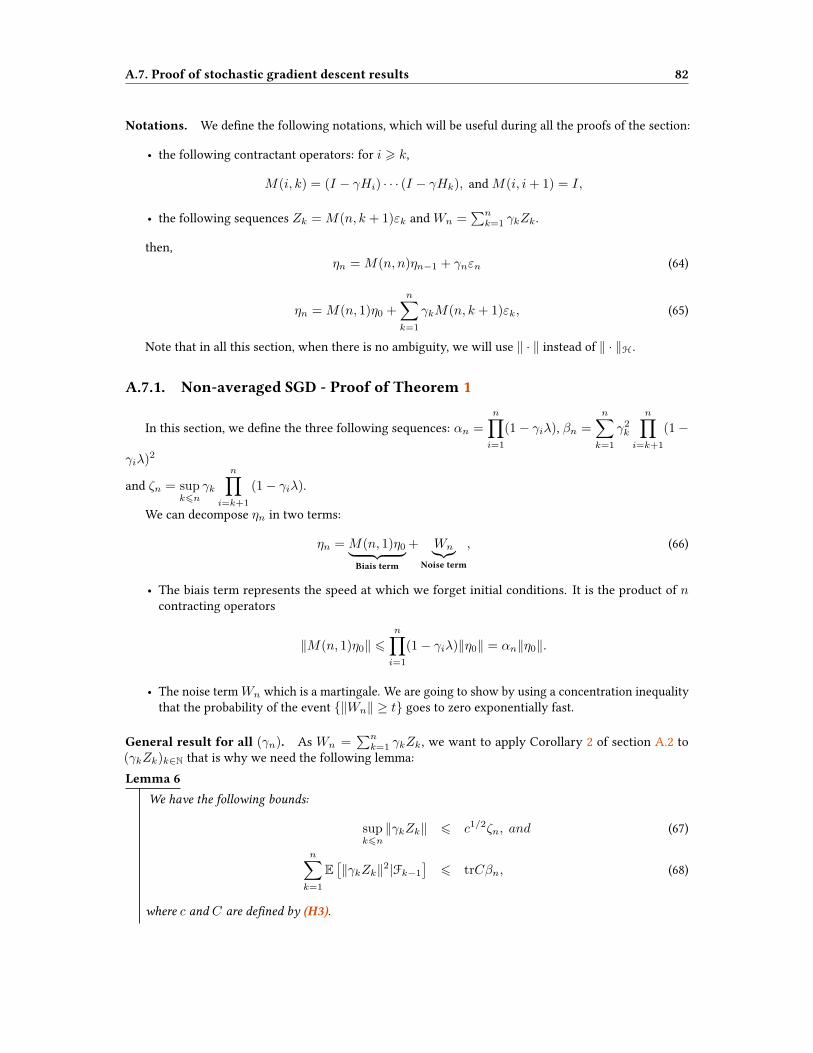
A.7. Proof of stochastic gradient descent results 82
Notations. We dene the following notations, which will be useful during all the proofs of the section:
• the following contractant operators: for i > k,
M(i, k) = (I − γHi) · · · (I − γHk), and M(i, i+ 1) = I,
• the following sequences Zk = M(n, k + 1)εk and Wn =∑nk=1 γkZk .
then,ηn = M(n, n)ηn−1 + γnεn (64)
ηn = M(n, 1)η0 +
n∑k=1
γkM(n, k + 1)εk, (65)
Note that in all this section, when there is no ambiguity, we will use ‖ · ‖ instead of ‖ · ‖H.
A.7.1. Non-averaged SGD - Proof of Theorem 1
In this section, we dene the three following sequences: αn =
n∏i=1
(1− γiλ), βn =
n∑k=1
γ2k
n∏i=k+1
(1−
γiλ)2
and ζn = supk6n
γk
n∏i=k+1
(1− γiλ).
We can decompose ηn in two terms:
ηn = M(n, 1)η0︸ ︷︷ ︸Biais term
+ Wn︸︷︷︸Noise term
, (66)
• The biais term represents the speed at which we forget initial conditions. It is the product of ncontracting operators
‖M(n, 1)η0‖ 6n∏i=1
(1− γiλ)‖η0‖ = αn‖η0‖.
• The noise term Wn which is a martingale. We are going to show by using a concentration inequalitythat the probability of the event ‖Wn‖ ≥ t goes to zero exponentially fast.
General result for all (γn). As Wn =∑nk=1 γkZk, we want to apply Corollary 2 of section A.2 to
(γkZk)k∈N that is why we need the following lemma:Lemma 6
We have the following bounds:
supk6n‖γkZk‖ 6 c1/2ζn, and (67)
n∑k=1
E[‖γkZk‖2|Fk−1
]6 trCβn, (68)
where c and C are dened by (H3).

A.7. Proof of stochastic gradient descent results 83
Proof : First, ‖γkZk‖ = γk ‖M(n, k + 1)εk‖ ≤ γk ‖M(n, k + 1)‖op ‖εk‖ ≤ γkαnαk‖εk‖ 6 ζnc
1/2.
Second,n∑k=1
E[‖γkZk‖2|Fk−1
]6
n∑k=1
α2n
α2k
γ2k E ‖εk‖2
6n∑k=1
α2n
α2k
γ2k trC.
Hence,n∑k=1
E[‖γkZk‖2|Fk−1
]6
n∑k=1
γ2k
n∏i=k+1
(1− γiλ)2trC
= trCβn.
Proposition 7
We have the following inequality: for t > 0, n > 1,
‖ηn‖ 6 αn‖η0‖+ Vn, with (69)
P (Vn > t) 6 2 exp
(− t2
2(trCβn + c1/2ζnt/3)
). (70)
Proof : We just need to apply Lemma 6 and Corollary 2 to the martingale Wn and Vn = ‖Wn‖ for all n.
Result for γn = γ/nα. We now derive estimates ofαn, βn and ζn to have explicit bound for the previousresult in the case where γn =
γ
nαfor α ∈ [0, 1]. Some of the estimations are taken from [BM11].
Lemma 7
In the interesting particular case where γn =γ
nαfor α ∈ [0, 1]:
• for α = 1, i.e γn =γ
n, then ζn =
γ
1− γλαn, and we have the following estimations for γλ <
1/2:
(i) αn 61
nγλ, (ii) βn 6
2(1− γλ)
1− 2γλ
4γλγ2
n2γλ, (iii) ζn 6
γ
(1− λγ)nγλ.
• for α = 0, i.e γn = γ, then ζn = γ, and we have the following:(i) αn = (1− γλ)n, (ii) βn 6
γ
λ, (iii) ζn = γ.
• for α ∈ ]0, 1[ , ζn = max
γn,
γ
1− γλαn
, and we have the following estimations:
(i) αn 6 exp
(− γλ
1− α((n+ 1)1−α − 1
)),
(ii) Denoting Lα = 2λγ1−α21−α
(1−
(34
)1−α), we distinguish three cases:
– α > 1/2, βn 6 γ2 2α2α−1 exp
(−Lαn1−α)+ 2αγ
λnα ,
– α = 1/2, βn 6 γ2 ln(3n) exp(−Lαn1−α)+ 2αγ
λnα ,

A.7. Proof of stochastic gradient descent results 84
– α < 1/2, βn 6 γ2 n1−2α
1−2α exp(−Lαn1−α)+ 2αγ
λnα .
(iii) ζn 6 max
γ1−γλ exp
(− γλ
1−α((n+ 1)1−α − 1
)), γnα
.
Note that in this case for n large enough we have the following estimations:
(i) αn 6 exp
(− γλ
21−α(1− α)n1−α
), (ii) βn 6
2α+1γ
λnα, (iii) ζn 6
γ
nα.
Proof : First we show for α ∈ [0, 1] the equality for ζn. Denote ak = γk∏ni=k+1(1 − γiλ), we want to nd
ζn = supk6n ak . We show for γn =γ
nαthat (ak)k>1 decreases then increases so that ζn = maxa1, an.
Let k 6 n− 1,
ak+1
ak=
γk+1
γk
1
(1− γk+1λ)
=1
γkγk+1
− γkλ
Hence, akak+1
− 1 =γkγk+1
− γkλ− 1. Take α ∈ ]0, 1[, in this case where γn =γ
nα,
akak+1
− 1 =
(1 +
1
k
)α− γλ
kα− 1.
A rapid study of the function fα(x) =
(1 +
1
x
)α− γλ
xα− 1 in R?+ shows that it decreases until
x? = (γλ)1
(α−1) − 1 then increases. This concludes the proof for α ∈ ]0, 1[. By a direct calculation forα = 1, ak
ak+1− 1 =
1− γλk
> 0 thus ak is non increasing and ζn = a1 =γ
1− γλαn. Similarly, for α = 0,akak+1
− 1 = γλ < 0 thus ak is increasing and ζn = an = γn.
We show now the dierent estimations we have for αn, βn and ζn for the three cases above.
• for α = 1,
lnαn =
n∑i=1
ln
(1− γλ
i
)6 −γλ
n∑i=1
1
i6 −γλ lnn
αn 61
nγλ.
Then,
βn = γ2n∑k=1
1
k2
n∏i=k+1
(1− γλ
i
)2
βn 6 γ2n∑k=1
1
k2exp
(−2γλ
n∑i=k+1
1
i
)
6 γ2n∑k=1
1
k2exp
(−2γλ ln
(n+ 1
k + 1
))
6 γ2n∑k=1
1
k2
(k + 1
n+ 1
)2γλ
6 4γλγ2n∑k=1
1
k2
(k
n
)2γλ
64γλγ2
n2γλ
n∑k=1
k2γλ−2,

A.7. Proof of stochastic gradient descent results 85
Moreover for γλ < 1
2,
n∑k=1
k2γλ−2 6 1− 1
2γλ− 1=
2(1− γλ)
1− 2γλ, hence,
βn 62(1− γλ)
1− 2γλ
4γλγ2
n2γλ
Finally,
ζn =γ
1− γλαn 6γ
1− γλ1
nγλ.
• for α = 0,
αn =
n∏i=1
(1− γλ) = (1− γλ)n.
Then,
βn = γ2n∑k=1
n∏i=k+1
(1− γλ)2 = γ2n∑k=1
(1− γλ)2(n−k) 61
1− (1− λγ)26γ
λ.
Finally,
ζn = γn = γ.
• for α ∈]0, 1[,
lnαn =
n∑i=1
ln
(1− γλ
iα
)6 −γλ
n∑i=1
1
iα6 −γλ (n+ 1)1−α − 1
1− α
αn 6 exp
(− γλ
1− α((n+ 1)1−α − 1
)).
To have an estimation on βn, we are going to split it into two sums. Let m ∈ J1, nK,
βn =
n∑k=1
γ2k
n∏i=k+1
(1− γiλ)2 =
m∑k=1
γ2k
n∏i=k+1
(1− γiλ)2 +
n∑k=m+1
γ2k
n∏i=k+1
(1− γiλ)2
βn 6m∑k=1
γ2k exp
(−2λ
n∑i=m+1
γi
)+γmλ
n∑k=m+1
n∏i=k+1
(1− γiλ)2 λγk
6n∑k=1
γ2k exp
(−2λ
n∑i=m+1
γi
)
+γmλ
n∑k=m+1
[n∏
i=k+1
(1− γiλ)2 −n∏
i=k+1
(1− γiλ)2 (1− γkλ)
]
6n∑k=1
γ2k exp
(−2λ
n∑i=m+1
γi
)+γmλ
n∑k=m+1
[n∏
i=k+1
(1− γiλ)2 −n∏i=k
(1− γiλ)2
]
6n∑k=1
γ2k exp
(−2λ
n∑i=m+1
γi
)+γmλ
(1−
n∏i=m+1
(1− γiλ)2
)
6n∑k=1
γ2k exp
(−2λ
n∑i=m+1
γi
)+γmλ.

A.7. Proof of stochastic gradient descent results 86
By taking γn =γ
nαand m = bn
2c, we get:
βn 6 γ2n∑k=1
1
k2αexp
−2λγ
n∑i=bn
2c+1
1
iα
+2αγ
λnα
6 γ2n∑k=1
1
k2αexp
(− 2λγ
1− α
((n+ 1)1−α −
(n2
+ 1)1−α
))+
2αγ
λnα
6 γ2n∑k=1
1
k2αexp
(− 2λγ
1− αn1−α
((1 +
1
n
)1−α
−(
1
2+
1
n
)1−α))
+2αγ
λnα
6 γ2n∑k=1
1
k2αexp
(− 2λγ
1− αn1−α21−α
(1−
(3
4
)1−α))
+2αγ
λnα.
Calling Sαn =∑nk=1
1k2α
and noting that: for α > 1/2, Sαn 6 2α2α−1
, α = 1/2, Sαn 6 ln(3n) andα < 1/2, Sαn 6 n1−2α
1−2αwe have the expected result.
Finally,
ζn 6 max
γ
1− γλ exp
(− γλ
1− α((n+ 1)1−α − 1
)),γ
nα
.
With this estimations we can easily show the Theorem 1. In the following we recall the main result ofthis Theorem and give an extension for α = 0 and α = 1 that cannot be found in the main text.Proposition 8 (SGD, decreasing step size: γn = γ/nα)
Assume (H1), (H2), (H3), γn = γ/nα, γλ < 1 and denote by ηn ∈ H the n-th iterate of the recursionin Eq. (57). We have for t > 0, n > 1,
• for α = 1 and γλ < 1/2, ‖gn − gλ‖H 6‖g0 − gλ‖H
nγλ+ Vn, almost surely, with
P (Vn > t) 6 2 exp
(− t2
43/2(trC)γ2/((1− 2γλ)nγλ) + 4tc1/2γ/3· nγλ
);
• for α = 0, ‖gn − gλ‖H 6 (1− γλ)n‖g0 − gλ‖H + Vn, almost surely, with
P (Vn > t) 6 2 exp
(− t2
2γ(trC/λ+ tc1/2/3)
);
• for α ∈ (0, 1), ‖gn − gλ‖H 6 exp(− γλ
1−α((n+ 1)1−α − 1
))‖g0 − gλ‖H + Vn, almost surely
for n large enough 5, with
P (Vn > t) 6 2 exp
(− t2
γ(2α+2trC/λ+ 2c1/2t/3)· nα
).
Proof of Theorem 1 : We apply Proposition 7, and the bound found on αn, βn and ζn in Lemma 7 to get theresults.
A.7.2. Averaged SGD for the variance term (η0 = 0) - Proof of Theorem 2
We consider the same recursion but with γn = γ:ηn = (I − γHn)ηn−1 + γεn,

A.7. Proof of stochastic gradient descent results 87
started at η0 = 0 and with assumptions (H1), (H2), (H3),(H4), (H5).However, in this section, we consider the averaged:
ηn =1
n+ 1
n∑i=0
ηi.
Thus, we get
ηn =1
n+ 1
n∑i=0
γ
i∑k=1
M(i, k + 1)εk =γ
n+ 1
n∑k=1
( n∑i=k
M(i, k + 1))εk =
γ
n+ 1
n∑k=1
Zk.
Our the goal is to bound P (‖ηn‖ > t) using Propostion 5 that is going to lead us to some Bernstein
concentration inquality. Calling, as above, Zk =
n∑i=k
M(i, k + 1)εk, and as E[Zk|Fk−1
]= 0 we just
need to bound, supk6n ‖Zk‖ and∑nk=1 E
[‖Zk‖2|Fk−1
]. For a more general result, we consider in the
following lemma (A1/2Zk)k .Lemma 8
Assuming (H1), (H2), (H3),(H4), (H5), we have the following bounds for Zk =
n∑i=k
M(i, k + 1)εk :
supk6n‖A1/2Zk‖ 6
c1/2‖A‖1/2op
γλ(71)
n∑k=1
E[‖A1/2Zk‖2|Fk−1
]6 n
1
γ2
1
1− γ/2γ0tr(AH−2 · C
). (72)
Proof : First ‖A1/2Zk‖ 6 ‖A‖1/2op ‖Zk‖ and we have, almost surely, ‖εk‖ 6 c1/2 and Hn < λI , thus for all k,as γλ 6 1, I − γHk 4 (1− γλ)I . Hence, ‖M(i, k + 1)‖op 6 (1− γλ)i−k and,
‖Zk‖ 6 ‖εk‖n∑i=k
‖M(i, k + 1)‖op 6 c1/2n∑i=k
(1− γλ)i−k 6c1/2
γλ
Second, we need an upper bound on E[‖A1/2Zk‖2|Fk−1
], we are going to nd it in two steps:
• Step 1: we rst show that the upper bound depends of the trace of some operator involving H−1.
E[‖A1/2Zk‖2|Fk−1
]6 2
n∑i=k
tr(A (γH)−1 E [M(i, k + 1)CM(i, k + 1)∗]
),
• Step 2: we then upperbound this sum to a telescopic one involving H−2 to nally show:
E[‖A1/2Zk‖2|Fk−1
]6
1
γ2
1
1− γ/2γ0tr(AH−2C
).
Step 1: We write,

A.7. Proof of stochastic gradient descent results 88
E[‖A1/2Zk‖2|Fk−1
]= E
∑k6i,j6n
⟨A1/2M(i, k + 1)εk, A
1/2M(j, k + 1)εk⟩|Fk−1
= E
∑k6i,j6n
〈M(i, k + 1)εk, AM(j, k + 1)εk〉 |Fk−1
=
∑k6i,j6n
E [tr (M(i, k + 1)∗AM(j, k + 1) · εk ⊗ εk)]
=∑
k6i,j6n
tr (E [M(i, k + 1)∗AM(j, k + 1)] · E [εk ⊗ εk]) .
We have E [εk ⊗ εk] 4 C so that as every operators are positive semi-denite,
E[‖A1/2Zk‖2|Fk−1
]6
∑k6i,j6n
tr (E [M(i, k + 1)∗AM(j, k + 1)] · C) .
We now bound the last expression by dividing it into two terms, noting M(i, k) = M ik for more compact
notations (only until the end of the proof),∑k6i,j6n
tr(E[M ik+1∗AM j
k+1
]· C)
=
n∑i=k
tr(E[M ik+1∗AM i
k+1
]· C)
+ 2∑
k6i<j6n
tr(E[M ik+1∗AM j
k+1
]· C).
Moreover, ∑k6i<j6n
tr(E[M ik+1∗AM j
k+1
]· C)
=∑
k6i<j6n
tr(E[M ik+1∗A (I − γH)j−iM i
k+1
]· C)
=
n∑i=k
tr
(E
[M ik+1∗A
n∑j=i+1
(I − γH)j−iM ik+1
]· C
)
=
n∑i=k
tr(E[M ik+1∗A[(I − γH)
(I − (I − γH)n−i
)(γH)−1
]M ik+1
]· C)
6n∑i=k
tr(E[M ik+1∗A[(γH)−1 − I
]M ik+1
]· C)
6n∑i=k
tr(E[M ik+1∗A (γH)−1 M i
k+1
]· C)−
n∑i=k
tr(E[M ik+1∗AM i
k+1
]· C).
Hence, ∑k6i,j6n
tr(E[M ik+1∗AM j
k+1
]· C)
=
n∑i=k
tr(E[M ik+1∗AM i
k+1
]· C)
+ 2∑
k6i<j6n
tr(E[M ik+1∗AM j
k+1
]· C)
6 2
n∑i=k
tr(E[M ik+1∗A (γH)−1 M i
k+1
]· C)−
n∑i=k
tr(E[M ik+1∗AM i
k+1
]· C)
6 2
n∑i=k
tr(E[M ik+1∗A (γH)−1 M i
k+1
]· C)
6 2
n∑i=k
tr(A (γH)−1 E
[M ik+1CM
ik+1∗])

A.7. Proof of stochastic gradient descent results 89
This concludes step 1.
Step 2: Let us now try to boundn∑i=k
tr(A (γH)−1 E
[M ik+1CM
ik+1∗])
. We will do so by bounding it
by a telescopic sum. Indeed,
E[M i+1k+1C (γH)−1 M i+1
k+1
∗]
= E[M ik+1 (I − γHi+1)C (γH)−1 (I − γHi+1)M i
k+1∗]
= E[M ik+1E
[C (γH)−1 − CH−1Hi+1 −Hi+1CH
−1 + γHi+1CH−1Hi+1
]M ik+1∗]
= E[M ik+1C (γH)−1 M i
k+1∗]− 2E
[M ik+1CM
ik+1∗]
+ γE[M ik+1E
[Hi+1CH
−1Hi+1
]M ik+1∗],
such that, by multiplying the previous equality by A (γH)−1 and taking the trace we have,
tr(A (γH)−1 E
[M i+1k+1C (γH)−1 M i+1
k+1
∗])
= tr(A (γH)−1 E
[M ik+1C (γH)−1 M i
k+1∗])
− 2tr(A (γH)−1 E
[M ik+1CM
ik+1∗])
+ γtr(A (γH)−1 E
[M ik+1E
[Hi+1CH
−1Hi+1
]M ik+1∗]),
And as E[HkCH
−1Hk]4 γ−1
0 C we have,
γtr(A (γH)−1 E
[M ik+1E
[Hi+1CH
−1Hi+1
]M ik+1∗])
6 γ/γ0tr(A (γH)−1 E
[M ik+1CM
ik+1∗]),
thus,
tr(A (γH)−1 E
[M i+1k+1C (γH)−1 M i+1
k+1
∗])
6 tr(A (γH)−1 E
[M ik+1C (γH)−1 M i
k+1∗])
− 2tr(A (γH)−1 E
[M ik+1CM
ik+1∗])
+ γ/γ0tr(A (γH)−1 E
[M ik+1CM
ik+1∗])
tr(A (γH)−1 E
[M ik+1CM
ik+1∗])
61
2− γγ0
(tr(A (γH)−1 E
[M ik+1C (γH)−1 M i
k+1∗])− tr
(A (γH)−1 E
[M i+1k+1C (γH)−1 M i+1
k+1
∗]))
.
If we take all the calculations from the beginning,
E[‖A1/2Zk‖2|Fk−1
]6
∑k6i,j6n
tr(E[M ik+1∗AM j
k+1
]· C)
6 2
n∑i=k
tr(A (γH)−1 E
[M ik+1CM
ik+1∗])
62
2− γ/γ0
n∑i=k
tr(A (γH)−1 E
[M ik+1C (γH)−1 M i
k+1∗])
−tr(A (γH)−1 E
[M i+1k+1C (γH)−1 M i+1
k+1
∗])
62
2− γ/γ0tr(A (γH)−1 E
[Mkk+1C (γH)−1 Mk
k+1
∗])6
1
γ2
1
1− γ/2γ0tr(AH−2 · C
),
which concludes the proof if we sum this inequality from 1 to n.
We can now prove Theorem 2:

A.7. Proof of stochastic gradient descent results 90
Proof of Theorem 2 : We apply Corollary 2 to the sequence(
γ
n+ 1A1/2Zk
)k6n
thanks to Lemma 8. We
have:
supk6n‖ γ
n+ 1A1/2Zk‖ 6
c1/2‖A1/2‖(n+ 1)λ
n∑k=1
E[‖ γ
n+ 1A1/2Zk‖2|Fk−1
]6
1
n+ 1
1
1− γ/2γ0tr(AH−2 · C
),
so that,
P(∥∥∥A1/2ηn
∥∥∥ > t)
= P
(∥∥∥∥∥n∑k=1
γ
n+ 1A1/2Zk
∥∥∥∥∥ > t
)6 2 exp
− t2
2
(tr(AH−2·C)
(n+1)(1−γ/2γ0)+ c1/2‖A1/2‖t
3λ(n+1)
)
P(∥∥∥A1/2ηn
∥∥∥ > t)6 2 exp
− (n+ 1)t2
2tr(AH−2·C)(1−γ/2γ0)
+ 2‖A1/2‖c1/2t3λ
.
A.7.3. Tail-averaged SGD - Proof of Corollary 1
We now prove the result for tail-averaging that allow us to relax the assumption that η0 = 0. Theproof relies on the fact that the bias term can easily be bounded as ‖ηtail, bias
n ‖H 6 (1− λγ)n/2‖η0‖H. Forthe variance term, we can simply use the Theorem 2 for n and n/2, as ηtail
n = 2ηn − ηn/2.Proof Proof of Corollary 1 : Let n > 1 and n an even number for the sake of clarity (the case where n is an
odd number can be solved similarly),
A1/2ηtailn =
1
n/2
n∑k=n/2
A1/2ηk
=1
n/2
n∑k=n/2
A1/2M(k, 1)η0 +1
n/2
n∑k=n/2
A1/2Wk
=1
n/2
n∑k=n/2
A1/2M(k, 1)η0 + 2A1/2Wn −A1/2Wn/2.
Hence,
∥∥∥A1/2ηtailn
∥∥∥ 6
∥∥∥∥∥∥ 1
n/2
n∑k=n/2
A1/2M(k, 1)η0
∥∥∥∥∥∥+ 2∥∥∥A1/2Wn
∥∥∥+∥∥∥A1/2Wn/2
∥∥∥6
1
n/2
n∑k=n/2
∥∥∥A1/2M(k, 1)∥∥∥op‖η0‖+ 2
∥∥∥A1/2Wn
∥∥∥+∥∥∥A1/2Wn/2
∥∥∥ ,Let Ln = 2
∥∥∥A1/2Wn
∥∥∥+∥∥∥A1/2Wn/2
∥∥∥,
∥∥∥A1/2ηtailn
∥∥∥ 61
n/2
n∑k=n/2
‖A1/2‖op(1− γλ)k ‖η0‖+ Ln∥∥∥A1/2ηtailn
∥∥∥ 6 (1− γλ)n/2‖A1/2‖op ‖η0‖+ Ln,

A.8. Exponentially convergent SGD for classication error 91
And nally for t > 0,
P(Ln > t) = P(2∥∥∥A1/2Wn
∥∥∥+∥∥∥A1/2Wn/2
∥∥∥ > t)
6 P(
2∥∥∥A1/2Wn
∥∥∥ > t)
+ P(∥∥∥A1/2Wn/2
∥∥∥ > t)
6 2
[exp
(− (n+ 1)(t/2)2
Et/2
)+ exp
(− (n/2 + 1)t2
Et
)].
Let us remark that Et/2 6 Et. Hence,
P(Ln > t) 6 2
[exp
(− (n+ 1)t2
4Et
)+ exp
(− (n+ 1)t2
2Et
)]6 4 exp
(− (n+ 1)t2
4Et
).
A.8. Exponentially convergent SGD for classification
error
In this section we prove the results for the error in the case of SGD. Let us recall the recursion:
gn − gλ =[I − γn(Kxn ⊗Kxn + λI)
](gn−1 − gλ) + γnεn,
with the noise term εk = ξkKxk + (g∗(xk)− gλ(xk))Kxk − E [(g∗(xk)− gλ(xk))Kxk ] ∈ H. This is thesame recursion as in Eq (57):
ηn = (I − γHn)ηn−1 + γnεn,
with Hn = Kxn ⊗Kxn + λI and ηn = gn − gλ. First we begin by showing that for this recursion andassuming (A2), (A3), we can show (H1), (H2), (H3),(H4).Lemma 9 (Showing (H1), (H2), (H3),(H4) for SGD recursion.)
Let us assume (A2), (A3),
• (H1) We start at some g0 − gλ ∈ H.
• (H2) (Hn, εn) i.i.d. andHn is a positive self-adjoint operator so that almost surelyHn < λI , withH = EHn = Σ + λI .
• (H3) We have the two following bounds on the noise:
‖εn‖ 6 R(1 + 2‖g∗ − gλ‖L∞) = c1/2
Eεn ⊗ εn 4 2(1 + ‖g∗ − gλ‖2∞
)Σ = C
E‖εn‖2 6 2(1 + ‖g∗ − gλ‖2∞
)trΣ = trC.
• (H4) We have:
E[HkCH
−1Hk
]4
(R2 + 2λ
)C = γ−1
0 C .

A.8. Exponentially convergent SGD for classication error 92
Proof : (H1), (H2) are obviously satised.Let us show (H3):
‖εn‖ = ‖ξnKxn + (g∗(xn)− gλ(xn))Kxn − E [(g∗(xn)− gλ(xn))Kxn ] ‖6 (|ξn|+ |g∗(xn)− gλ(xn)|)‖Kxn‖+ E [|g∗(xn)− gλ(xn)|‖Kxn‖]6 (1 + ‖g∗ − gλ‖∞)R+ ‖g∗ − gλ‖∞R= R(1 + 2‖g∗ − gλ‖∞)
We have 6:
εn ⊗ εn 4 2ξnKxn ⊗ ξnKxn + 2 ((g∗(xn)− gλ(xn))Kxn − E [(g∗(xn)− gλ(xn))Kxn ])
⊗ ((g∗(xn)− gλ(xn))Kxn − E [(g∗(xn)− gλ(xn))Kxn ])
Moreover, E[ξnKxn ⊗ ξnKxn ] = E[ξ2nKxn ⊗Kxn ] 4 Σ, And,
E[((g∗(xn)− gλ(xn))Kxn − E [(g∗(xn)− gλ(xn)Kxn ])
⊗ ((g∗(xn)− gλ(xn))Kxn − E [(g∗(xn)− gλ(xn))Kxn ])]
= E[(g∗(xn)− gλ(xn))2(xn)Kxn ⊗Kxn
]− E [(g∗(xn)− gλ(xn))Kxn ]
⊗ E [(g∗(xn)− gλ(xn))Kxn ]
4 E[(g∗(xn)− gλ(xn))2(xn)Kxn ⊗Kxn
]4 ‖g∗ − gλ‖2∞Σ.
So that,Eεn ⊗ εn 4 2
(1 + ‖g∗ − gλ‖2∞
)Σ
Finally Eεn ⊗ εn 4 2(1 + ‖g∗ − gλ‖2∞
)Σ, we have trEεn ⊗ εn 6 2
(1 + ‖g∗ − gλ‖2∞
)trΣ, thus
trEεn ⊗ εn = Etrεn ⊗ εn = E‖εn‖2 6 2(1 + ‖g∗ − gλ‖2∞
)trΣ.
To conclude the proof of this lemma, let us show (H4). We have:
E[(Kxk ⊗Kxk + λI)Σ(Σ + λI)−1(Kxk ⊗Kxk + λI)
]= E
[Kxk ⊗KxkΣ(Σ + λI)−1Kxk ⊗Kxk
]+ λΣΣ(Σ + λI)−1 + λΣ
Moreover, λΣΣ(Σ +λI)−1 = λΣ(Σ +λI−λI)(Σ +λI)−1 = λΣ−λ2Σ(Σ +λI)−1 4 λΣ, and similarly,E[Kxk⊗KxkΣ(Σ+λI)−1Kxk⊗Kxk
]= E
[(Kxk⊗Kxk )2
]−λE
[Kxk⊗Kxk (Σ+λI)−1Kxk⊗Kxk
]4
R2Σ.Finally we obtain E
[(Kxk ⊗ Kxk + λI)Σ(Σ + λI)−1(Kxk ⊗ Kxk + λI)
]4 R2Σ + λΣ + λΣ =
(R2 + 2λ)Σ.
A.8.1. SGD with decreasing step-size: proof of Theorem 3
Proof of Theorem 3 : Let us apply Theorem 1 to gn − gλ. We assume (A2), (A3) and A = I , such that (A2),(A3), we can show that (H1), (H2), (H3),(H4), (H5) are veried (Lemma 9). Let δ correspond to the one of(A4). We have for t = δ/(4R), n > 1:
‖gn − gλ‖H 6 exp
(− γλ
1− α((n+ 1)1−α − 1
))‖g0 − gλ‖H + ‖Wn‖H, a.s, with
P (‖Wn‖H > δ/(4R)) 6 2 exp
(− δ2
CRnα), CR = γ(2α+6R2trC/λ+ 8Rc1/2δ/3).
6We use the following inequality: for all a and b ∈ H, (a + b) ⊗ (a + b) 4 2a ⊗ a + 2b ⊗ b. Indeed, for all x ∈ H,〈x, (a+ b)⊗ (a+ b)x〉 = (〈a+ b, x〉)2 = (〈a, x〉+ 〈b, x〉)2 6 2〈a, x〉2 + 2〈b, x〉2 = 2〈x, (a⊗ a)x〉+ 2〈x, (b⊗ b)x〉.

A.9. Extension of Corollary 1 and Theorem 4 for the full averaged case. 93
Then if n is such that exp(− γλ
1−α
((n+ 1)1−α − 1
))6
δ
5R‖g0 − gλ‖H,
‖gn − gλ‖H 6δ
5R+
δ
4R, with probability 1− 2 exp
(− δ2
CRnα),
‖gn − gλ‖H <δ
2R, with probability 1− 2 exp
(− δ2
CRnα).
Now assume (A1), (A4), we simply apply Lemma 1 to gn with q = 2 exp(− δ2
CRnα)
And
CR = γ(2α+6R2trC/λ+ 8Rc1/2δ/3)
CR == γ
(2α+7R2trΣ
(1 + ‖g∗ − gλ‖2∞
)λ
+8R2δ(1 + 2‖g∗ − gλ‖∞)
3
).
A.8.2. Tail averaged SGD with constant step-size: proof of Theorem 4
Proof of Theorem 4 : Let us apply Corollary 1 to gn − gλ. We assume (A2), (A3) and A = I , such that(H1), (H2), (H3),(H4), (H5) are veried (Lemma 9). Let δ correspond to the one of (A4). We have fort = δ/(4R), n > 1: ∥∥∥gtail
n − gλ∥∥∥H
6 (1− γλ)n/2‖g0 − gλ‖H + Ln ,with
P(Ln > t) 6 4 exp(−(n+ 1)t2/(4Et)
).
Then as soon as (1− γλ)n/2 6δ
5R‖g0 − gλ‖H,
∥∥∥gtailn − gλ
∥∥∥H
6δ
5R+
δ
4R, with probability 1− 4 exp
(−(n+ 1)δ2/(64R2Eδ/(4R))
),∥∥∥gtail
n − gλ∥∥∥H
<δ
2R, with probability 1− 4 exp
(−(n+ 1)δ2/(64R2Eδ/(4R))
).
Now assume (A1), (A4), we simply apply Lemma 1 to gtailn with q = 4 exp
(−(n+ 1)δ2/KR)
). And
KR = 64R2Eδ/(4R) = 64R2
(4tr(H−2C) +
2c1/2
3λ· δ
4R
)= 512R2 (1 + ‖g∗ − gλ‖2∞
)tr((Σ + λI)−2Σ) +
32δR2(1 + 2‖g∗ − gλ‖∞)
3λ.
A.9. Extension of Corollary 1 and Theorem 4 for the full
averaged case.
A.9.1. Extension of Corollary 1 for the full averaged case.
Let us recall the SGD abstract recursion dened in Eq. (57) that we are going to further apply withηn = gn − gλ, Hn = Kxn ⊗Kxn + λI and H = Σ + λI :
ηn = (I − γHn)ηn−1 + γnεn,
ηn = M(n, 1)η0︸ ︷︷ ︸ηbiasn
+
n∑k=1
γkM(n, k + 1)εk︸ ︷︷ ︸ηvariancen
.
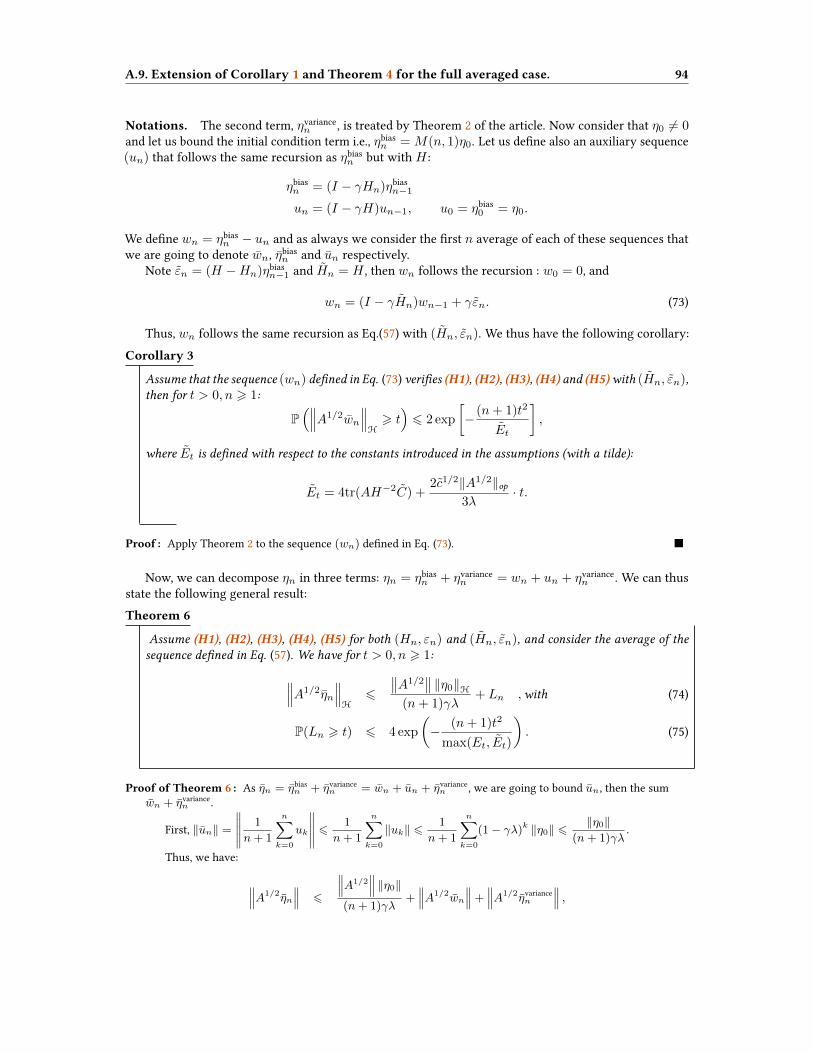
A.9. Extension of Corollary 1 and Theorem 4 for the full averaged case. 94
Notations. The second term, ηvariancen , is treated by Theorem 2 of the article. Now consider that η0 6= 0
and let us bound the initial condition term i.e., ηbiasn = M(n, 1)η0. Let us dene also an auxiliary sequence
(un) that follows the same recursion as ηbiasn but with H :
ηbiasn = (I − γHn)ηbias
n−1
un = (I − γH)un−1, u0 = ηbias0 = η0.
We dene wn = ηbiasn − un and as always we consider the rst n average of each of these sequences that
we are going to denote wn, ηbiasn and un respectively.
Note εn = (H −Hn)ηbiasn−1 and Hn = H , then wn follows the recursion : w0 = 0, and
wn = (I − γHn)wn−1 + γεn. (73)
Thus, wn follows the same recursion as Eq.(57) with (Hn, εn). We thus have the following corollary:Corollary 3
Assume that the sequence (wn) dened in Eq. (73) veries (H1), (H2), (H3), (H4) and (H5)with (Hn, εn),then for t > 0, n > 1:
P(∥∥∥A1/2wn
∥∥∥H
> t)6 2 exp
[− (n+ 1)t2
Et
],
where Et is dened with respect to the constants introduced in the assumptions (with a tilde):
Et = 4tr(AH−2C) +2c1/2‖A1/2‖op
3λ· t.
Proof : Apply Theorem 2 to the sequence (wn) dened in Eq. (73).
Now, we can decompose ηn in three terms: ηn = ηbiasn + ηvariance
n = wn + un + ηvariancen . We can thus
state the following general result:Theorem 6
Assume (H1), (H2), (H3), (H4), (H5) for both (Hn, εn) and (Hn, εn), and consider the average of thesequence dened in Eq. (57). We have for t > 0, n > 1:∥∥∥A1/2ηn
∥∥∥H
6
∥∥A1/2∥∥ ‖η0‖H
(n+ 1)γλ+ Ln ,with (74)
P(Ln > t) 6 4 exp
(− (n+ 1)t2
max(Et, Et)
). (75)
Proof of Theorem 6 : As ηn = ηbiasn + ηvariance
n = wn + un + ηvariancen , we are going to bound un, then the sum
wn + ηvariancen .
First, ‖un‖ =
∥∥∥∥∥ 1
n+ 1
n∑k=0
uk
∥∥∥∥∥ 61
n+ 1
n∑k=0
‖uk‖ 61
n+ 1
n∑k=0
(1− γλ)k ‖η0‖ 6‖η0‖
(n+ 1)γλ.
Thus, we have:
∥∥∥A1/2ηn
∥∥∥ 6
∥∥∥A1/2∥∥∥ ‖η0‖
(n+ 1)γλ+∥∥∥A1/2wn
∥∥∥+∥∥∥A1/2ηvariance
n
∥∥∥ ,
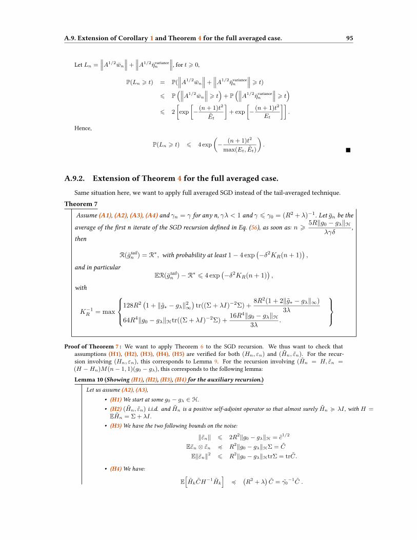
A.9. Extension of Corollary 1 and Theorem 4 for the full averaged case. 95
Let Ln =∥∥∥A1/2wn
∥∥∥+∥∥∥A1/2ηvariance
n
∥∥∥, for t > 0,
P(Ln > t) = P(∥∥∥A1/2wn
∥∥∥+∥∥∥A1/2ηvariance
n
∥∥∥ > t)
6 P(∥∥∥A1/2wn
∥∥∥ > t)
+ P(∥∥∥A1/2ηvariance
n
∥∥∥ > t)
6 2
[exp
[− (n+ 1)t2
Et
]+ exp
[− (n+ 1)t2
Et
]].
Hence,
P(Ln > t) 6 4 exp
(− (n+ 1)t2
max(Et, Et)
).
A.9.2. Extension of Theorem 4 for the full averaged case.
Same situation here, we want to apply full averaged SGD instead of the tail-averaged technique.Theorem 7
Assume (A1), (A2), (A3), (A4) and γn = γ for any n, γλ < 1 and γ 6 γ0 = (R2 + λ)−1. Let gn be the
average of the rst n iterate of the SGD recursion dened in Eq. (56), as soon as: n >5R‖g0 − gλ‖H
λγδ,
then
R(gtailn ) = R∗, with probability at least 1− 4 exp(−δ2KR(n+ 1)
),
and in particularER(gtailn )− R∗ 6 4 exp
(−δ2KR(n+ 1)
),
with
K−1R = max
128R2
(1 + ‖g∗ − gλ‖2∞
)tr((Σ + λI)−2Σ) +
8R2(1 + 2‖g∗ − gλ‖∞)
3λ
64R4‖g0 − gλ‖Htr((Σ + λI)−2Σ) +16R4‖g0 − gλ‖H
3λ.
Proof of Theorem 7 : We want to apply Theorem 6 to the SGD recursion. We thus want to check that
assumptions (H1), (H2), (H3), (H4), (H5) are veried for both (Hn, εn) and (Hn, εn). For the recur-sion involving (Hn, εn), this corresponds to Lemma 9. For the recursion involving (Hn = H, εn =(H −Hn)M(n− 1, 1)(g0 − gλ), this corresponds to the following lemma:
Lemma 10 (Showing (H1), (H2), (H3), (H4) for the auxiliary recursion.)
Let us assume (A2), (A3),
• (H1)We start at some g0 − gλ ∈ H.
• (H2) (Hn, εn) i.i.d. and Hn is a positive self-adjoint operator so that almost surely Hn < λI , with H =EHn = Σ + λI .
• (H3)We have the two following bounds on the noise:
‖εn‖ 6 2R2‖g0 − gλ‖H = c1/2
Eεn ⊗ εn 4 R2‖g0 − gλ‖HΣ = C
E‖εn‖2 6 R2‖g0 − gλ‖HtrΣ = trC.
• (H4)We have:
E[HkCH
−1Hk]
4(R2 + λ
)C = γ0
−1C .

A.9. Extension of Corollary 1 and Theorem 4 for the full averaged case. 96
Proof : (H1), (H2) are obviously satised.Let us show (H3): For the rst one:
‖εn‖ = ‖(H −Hn)M(n− 1, 1)(g0 − gλ)‖6 ‖(Σ−Kxn ⊗Kxn)‖ ‖M(n− 1, 1)‖ ‖g0 − gλ‖
6 2R2‖g0 − gλ‖H.
‖εn‖ = ‖(H −Hn)M(n− 1, 1)(g0 − gλ)‖6 ‖(Σ−Kxn ⊗Kxn)‖ ‖M(n− 1, 1)‖ ‖g0 − gλ‖
6 2R2‖g0 − gλ‖H.
And for the second inquality:
E [εn ⊗ εn|Fn−1] = E[(Σ−Kxn ⊗Kxn) ηbias
n ⊗ ηbiasn (Σ−Kxn ⊗Kxn) |Fn−1
]= Σηbias
n ⊗ ηbiasn Σ− 2Σηbias
n ⊗ ηbiasn Σ + E
[Kxn ⊗Kxnη
biasn ⊗ ηbias
n Kxn ⊗Kxn
]= −Σηbias
n ⊗ ηbiasn Σ + E
[〈Kxn , η
biasn 〉2Kxn ⊗Kxn
]4 R2‖g0 − gλ‖HΣ.
Finally, we have for (H4) :
E[HkCH
−1Hk]
= HC = R2‖g0 − gλ‖H(Σ2 + λΣ) 4 R2‖g0 − gλ‖H(‖Σ‖op + λ)Σ
4(R2 + λ
)C = γ0
−1C.
Let us apply now Theorem 6 to gn − gλ. We assume (A2), (A3) and A = I , such that (H1), (H2), (H3),(H4), (H5) are veried for both problems ((Hn, εn) and (Hn, εn)) (Lemma 9,10). Let δ correspond to the oneof Assumption (A4). We have for t = δ/(4R), n > 1:
‖gn − gλ‖H 6‖g0 − gλ‖H(n+ 1)γλ
+ Ln ,with
P(Ln > t) 6 4 exp
(− (n+ 1)t2
max(Et, Et)
).
Then as soon as 1
(n+ 1)λγ6
δ
5R‖g0 − gλ‖H,
‖gn − gλ‖H 6δ
5R+
δ
4R, with probability 1− 4 exp
(− (n+ 1)δ2
16R2 max(Eδ/4R, Eδ/4R)
),
‖gn − gλ‖H <δ
2R, with probability 1− 4 exp
(− (n+ 1)δ2
16R2 max(Eδ/4R, Eδ/4R)
).
Now assume (A1), (A4), we now only have to apply Lemma 1 to the estimator gn with the probability
q = 4 exp
(− (n+ 1)δ2
16R2 max(Eδ/4R, Eδ/4R)
). And,
K−1R = 16R2 max(Eδ/4R, Eδ/4R)
= max
128R2 (1 + ‖g∗ − gλ‖2∞
)tr((Σ + λI)−2Σ) +
8R2(1 + 2‖g∗ − gλ‖∞)
3λ
64R4‖g0 − gλ‖Htr((Σ + λI)−2Σ) +16R4‖g0 − gλ‖H
3λ.

A.10. Convergence rate under weaker margin assumption 97
A.10. Convergence rate under weaker margin assumption
We make the following assumptions:
(A7) ∀δ > 0, P (|g∗| 6 2δ) 6 δα.
(A8) There exists 7 γ > 0 such that ∀λ > 0, ‖g∗ − gλ‖∞ 6 λγ .
(A9) The eigenvalues of Σ decrease as 1/nβ for β > 1.
Note that (A7) is weaker than (A1) and to balance this we need a stronger condition on gλ than (A4)
which is (A8). (A9) is just a technical assumption needed to give explicit rate. The following Corollarycorresponds to Theorem 4 with the new assumptions. Note that it could also be shown for the full averagesequence gn.Corollary 4 (Explicit onvergence rate under weaker margin condition)
Assume (A2), (A3), (A7), (A8) and (A9). Let γn = γ for any n, γλ < 1 and γ 6 γ0 = (R2 + 2λ)−1.Let gtailn be the n-th iterate of the recursion dened in Eq. (56), and gtailn = 1
bn/2c∑ni=bn/2c gi, as soon as
n >2
γλln(
5R‖g0 − gλ‖Hδ
), then
E[R(gtailn )−R∗
]6
Cα,βnα·qγ,β
.
Proof : The proof technique follows the one of [AT07].Let δ, λ > 0, such that ‖g∗ − gλ‖∞ 6 δ. Remark that ∀j ∈ N,P(sign(g∗(X))gλ(X) 6 2jδ
)6 P
(|gλ(X)| 6 2jδ
)6 P
(|g∗(X)| 6 2j+1δ
)6 2αjδα.
Note A0 = x ∈ X| sign(g∗)gλ 6 δ and for j > 1, Aj = x ∈ X| 2j−1δ < sign(g∗)gλ 6 2jδ. Then,
E[R(gtail
n )−R∗]
=∑j∈N
E[(R(gtail
n )−R∗)1Aj
]= E
[(R(gtail
n )−R∗)1sign(g∗)gλ6δ
]+∑j>1
E[(R(gtail
n )−R∗)1Aj
]6 P (sign(g∗(X))gλ(X) 6 δ) +
∑j>1
E[(R(gtail
n )−R∗)12j−1δ<sign(g∗(X))gλ(X)62jδ
]
6 δα +∑j>1
EX
Ex1,...,xn(R(gtail
n )−R∗)12j−1δ<sign(g∗(X))gλ(X)︸ ︷︷ ︸Theorem 4
|x1, . . . , xn
·1sign(g∗(X))gλ(X)62jδ
]6 δα + 4
∑j>1
P(
sign(g∗(X))gλ(X) 6 2jδ)
exp(−(2jδ)2KR(δ)(n+ 1)
)6 δα + 4δα
∑j>1
2αj exp(−(2jδ)2KR(δ)(n+ 1)
),
and KR(δ)−1 = 29R2 (1 + ‖g∗ − gλ‖2∞)
tr(Σ(Σ + λI)−2) +32δR2(1 + 2‖g∗ − gλ‖∞)
3λ. Let us now
choose δ as a function of n to cancel the dependence on n in the exponential term. In the following, as we7This assumption is veried for the following source condition ∃g ∈ H, r > 0 s.t. PH(g) = Σrg∗. If the additionnal assumption
(A9) is veried then (A8) is veried with γ =r−1/2
2r+1/β[CDV07].

A.10. Convergence rate under weaker margin assumption 98
assumed (A8), we chose λ = δ1/γ such that ‖g∗ − gλ‖∞ 6 λγ = δ. Second, (A9) implies (see [CDV07]) thattr(Σ(Σ + λI)−2) 6
β
(β − 1)λ1+1/β. For δ small enough, we have:
KR(δ)−1 6 210 βR2
(β − 1)δ1+1/βγ
+ 32δ(γ−1)/γR2
KR(δ)−1 6 211 βR2
(β − 1)· δ−(β+1)/βγ
Hence, if we take δ2δ(β+1)/βγ = 1/n, i.e., δ = n−γ/(2γ+1+1/β), we have:
E[R(gtail
n )−R∗]6
1 +∑j>1 2αj+2 exp
(−4j(β − 1)/(211βR2)
)nαγ/(2γ+1+1/β)
.
As the sum converges, we have proved the result.
?
? ?

This is a fucking blank sentence.
99

2. StatisticalOptimalityof SGDonHard
LearningProblemsthroughMultiple
Passes
2.1. Introduction
Stochastic gradient descent (SGD) and its multiple variants —averaged [PJ92], accelerated [Lan12],variance-reduced [RSB12, JZ13, DBLJ14]— are the workhorses of large-scale machine learning, because (a)these methods looks at only a few observations before updating the corresponding model, and (b) they areknown in theory and in practice to generalize well to unseen data [BCN18].
Beyond the choice of step-size (often referred to as the learning rate), the number of passes to make onthe data remains an important practical and theoretical issue. In the context of nite-dimensional models(least-squares regression or logistic regression), the theoretical answer has been known for many years: asingle passes suces for the optimal statistical performance [PJ92, NY83]. Worse, most of the theoreticalwork only apply to single pass algorithms, with some exceptions leading to analyses of multiple passeswhen the step-size is taken smaller than the best known setting [HRS16, LR17].
However, in practice, multiple passes are always performed as they empirically lead to better general-ization (e.g., loss on unseen test data) [BCN18]. But no analysis so far has been able to show that, giventhe appropriate step-size, multiple pass SGD was theoretically better than single pass SGD.
The main contribution of this paper is to show that for least-squares regression, while single passaveraged SGD is optimal for a certain class of “easy” problems, multiple passes are needed to reach optimalprediction performance on another class of “hard” problems.
In order to dene and characterize these classes of problems, we need to use tools from innite-dimensional models which are common in the analysis of kernel methods. De facto, our analysis will bedone in innite-dimensional feature spaces, and for nite-dimensional problems where the dimensionfar exceeds the number of samples, using these tools are the only way to obtain non-vacuous dimension-independent bounds. Thus, overall, our analysis applies both to nite-dimensional models with explicitfeatures (parametric estimation), and to kernel methods (non-parametric estimation).
The two important quantities in the analysis are:
(a) The decay of eigenvalues of the covariance matrix Σ of the input features, so that the orderedeigenvalues λm decay as O(m−α); the parameter α > 1 characterizes the size of the feature space,α = 1 corresponding to the largest feature spaces and α = +∞ to nite-dimensional spaces. Thedecay will be measured through trΣ1/α =
∑m λ
1/αm , which is small when the decay of eigenvalues
is faster than O(m−α).
(b) The complexity of the optimal predictor θ∗ as measured through the covariance matrix Σ, thatis with coecients 〈em, θ∗〉 in the eigenbasis (em)m of the covariance matrix that decay so that〈θ∗,Σ1−2rθ∗〉 is small. The parameter r > 0 characterizes the diculty of the learning problem:r = 1/2 corresponds to characterizing the complexity of the predictor through the squared norm‖θ∗‖2, and thus r close to zero corresponds to the hardest problems while r larger, and in particularr > 1/2, corresponds to simpler problems.
Dealing with non-parametric estimation provides a simple way to evaluate the optimality of learningprocedures. Indeed, given problems with parameters r and α, the best prediction performance (averagedsquare loss on unseen data) is well known [FS17] and decay as O(n
−2rα2rα+1 ), with α = +∞ leading to the
usual parametric rate O(n−1). For easy problems, that is for which r > α−12α , then it is known that most
iterative algorithms achieve this optimal rate of convergence (but with various running-time complexities),
100

2.2. Least-squares regression in nite dimension 101
such as exact regularized risk minimization [CDV07], gradient descent on the empirical risk [YRC07], oraveraged stochastic gradient descent [DB16].
We show that for hard problems, that is for which r 6 α−12α (see Example 2 for a typical hard problem),
then multiple passes are superior to a single pass. More precisely, under additional assumptions detailedin Section 2.2 that will lead to a subset of the hard problems, with Θ(n(α−1−2rα)/(1+2rα)) passes, weachieve the optimal statistical performance O(n
−2rα2rα+1 ), while for all other hard problems, a single pass
only achieves O(n−2r). This is illustrated in Figure 13.We thus get a number of passes that grows with the number of observations n and depends precisely
on the quantities r and α. In synthetic experiments with kernel methods where α and r are known, thesescalings are precisely observed. In experiments on parametric models with large dimensions, we alsoexhibit an increasing number of required passes when the number of observations increases.
1 2 3 4 5 6 7 8 9 100.0
0.2
0.4
0.6
0.8
1.0
r
Hard Problems
Easy Problems r = 1
2
1 2 3 4 5 6 7 8 9 100.0
0.2
0.4
0.6
0.8
1.0
rOptimal rates with multiple passes
Optimal rates with one pass
Improved rateswith multiple passes
r = 12
Figure 13 – (Left) easy and hard problems in the (α, r)-plane. (Right) dierent regions for which multiplepasses improved known previous bounds (green region) or reaches optimality (red region).
2.2. Least-sqares regression in finite dimension
We consider a joint distribution ρ on pairs of input/output (x, y) ∈ X×R, where X is any input space,and we consider a feature map Φ from the input space X to a feature space H, which we assume Euclideanin this section, so that all quantities are well-dened. In Section 2.4, we will extend all the notions toHilbert spaces.
2.2.1. Main assumptions
We are considering predicting y as a linear function fθ(x) = 〈θ,Φ(x)〉H of Φ(x), that is estimatingθ ∈ H such that F (θ) = 1
2E(y − 〈θ,Φ(x)〉H)2 is as small as possible. Estimators will depend on nobservations, with standard sampling assumptions:
(A6) The n observations (xi, yi) ∈ X×R, i = 1, . . . , n, are independent and identically distributed fromthe distribution ρ.
Since H is nite-dimensional, F always has a (potentially non-unique) minimizer in H which wedenote θ∗. We make the following standard boundedness assumptions:
(A7) ‖Φ(x)‖ 6 R almost surely, |y−〈θ∗,Φ(x)〉H| is almost surely bounded by σ and |y| is almost surelybounded byM .

2.2. Least-squares regression in nite dimension 102
In order to obtain improved rates with multiple passes, and motivated by the equivalent previouslyused condition in reproducing kernel Hilbert spaces presented in Section 2.4, we make the following extraassumption (we denote by Σ = E[Φ(x)⊗H Φ(x)] the (non-centered) covariance matrix).
(A8) For µ ∈ [0, 1], there exists κµ > 0 such that, almost surely, Φ(x)⊗H Φ(x) 4H κ2µR
2µΣ1−µ. Notethat it can also be written as ‖Σµ/2−1/2Φ(x)‖H 6 κµR
µ.
Assumption (A8) is always satised with any µ ∈ [0, 1], and has particular values for µ = 1, withκ1 = 1, and µ = 0, where κ0 has to be larger than the dimension of the space H.
We will also introduce a parameter α that characterizes the decay of eigenvalues of Σ through thequantity trΣ1/α, as well as the diculty of the learning problem through ‖Σ1/2−rθ∗‖H, for r ∈ [0, 1]. Inthe nite-dimensional case, these quantities can always be dened and most often nite, but may be verylarge compared to sample size. In the following assumptions the quantities are assumed to be nite andsmall compared to n.
(A9) There exists α > 1 such that tr Σ1/α <∞.
Assumption (A9) is often called the “capacity condition”. First note that this assumption impliesthat the decreasing sequence of the eigenvalues of Σ, (λm)m>1, satises λm = o (1/mα). Note thattrΣµ 6 κ2
µR2µ and thus often we have µ > 1/α, and in the most favorable cases in Section 2.4, this bound
will be achieved. We also assume:
(A10) There exists r > 0, such that ‖Σ1/2−rθ∗‖H <∞.
Assumption (A10) is often called the “source condition”. Note also that for r = 1/2, this simply saysthat the optimal predictor has a small norm.
In the subsequent sections, we essentially assume that α, µ and r are chosen (by the theoretical analysis,not by the algorithm) so that all quantities Rµ, ‖Σ1/2−rθ∗‖H and trΣ1/α are nite and small. As recalledin the introduction, these parameters are often used in the non-parametric literature to quantify thehardness of the learning problem (Figure 13).
We will use result with O(·) and Θ(·) notations, which will all be independent of n and t (numberof observations and number of iterations) but can depend on other nite constants. Explicit dependenceon all parameters of the problem is given in proofs. More precisely, we will use the usual O(·) and Θ(·)notations for sequences bnt and ant that can depend on n and t, as ant = O(bnt) if and only if, there existsM > 0 such that for all n, t, ant 6 Mbnt, and ant = Θ(bnt) if and only if, there exist M,M ′ > 0 suchthat for all n, t, M ′bnt 6 ant 6Mbnt.
2.2.2. Related work
Given our assumptions above, several algorithms have been developed for obtaining low values of theexpected excess risk E
[F (θ)
]− F (θ∗).
Regularized empirical risk minimization. Forming the empirical risk F (θ), it minimizes F (θ) +λ‖θ‖2H, for appropriate values of λ. It is known that for easy problems where r > α−1
2α , it achieves theoptimal rate of convergence O(n
−2rα2rα+1 ) [CDV07]. However, algorithmically, this requires to solve a linear
system of size n times the dimension of H. One could also use fast variance-reduced stochastic gradientalgorithms such as SAG [RSB12], SVRG [JZ13] or SAGA [DBLJ14], with a complexity proportional to thedimension of H times n+R2/λ.
Early-stopped gradient descent on the empirical risk. Instead of solving the linear system directly,one can use gradient descent with early stopping [YRC07, LRRC18]. Similarly to the regularized empiricalrisk minimization case, a rate of O(n−
2rα2rα+1 ) is achieved for the easy problems, where r > α−1
2α . Dierent

2.3. Averaged SGD with multiple passes 103
iterative regularization techniques beyond batch gradient descent with early stopping have been considered,with computational complexities ranging from O(n1+ α
2rα+1 ) to O(n1+ α4rα+2 ) times the dimension of H
(or n in the kernel case in Section 2.4) for optimal predictions [YRC07, GRO+08, RV15, BK16, LRRC18].
Stochastic gradient. The usual stochastic gradient recursion is iterating from i = 1 to n,
θi = θi−1 + γ(yi − 〈θi−1,Φ(xi)〉H
)Φ(xi),
with the averaged iterate θn = 1n
∑ni=1 θi. Starting from θ0 = 0, [BM13] shows that the expected excess
performance E[F (θn)] − F (θ∗) decomposes into a variance term that depends on the noise σ2 in theprediction problem, and a bias term, that depends on the deviation θ∗ − θ0 = θ∗ between the initializationand the optimal predictor. Their bound is, up to universal constants, σ
2dim(H)n +
‖θ∗‖2Hγn .
Further, [DB16] considered the quantities α and r above to get the bound, up to constant factors:
σ2trΣ1/α(γn)1/α
n+‖Σ1/2−rθ∗‖2
γ2rn2r.
We recover the nite-dimensional bound for α = +∞ and r = 1/2. The bounds above are valid for allα > 1 and all r ∈ [0, 1], and the step-size γ is such that γR2 6 1/4, and thus we see a natural trade-oappearing for the step-size γ, between bias and variance.
When r > α−12α , then the optimal step-size minimizing the bound above is γ ∝ n
−2αminr,1−1+α2αminr,1+1 , and
the obtained rate is optimal. Thus a single pass is optimal. However, when r 6 α−12α , the best step-size
does not depend on n, and one can only achieve O(n−2r).Finally, in the same multiple pass set-up as ours, [LR17] has shown that for easy problems where
r > α−12α (and single-pass averaged SGD is already optimal) that multiple-pass non-averaged SGD is
becoming optimal after a correct number of passes (while single-pass is not). Our proof principle ofcomparing to batch gradient is taken from [LR17], but we apply it to harder problems where r 6 α−1
2α .Moreover we consider the multi-pass averaged-SGD algorithm, instead of non-averaged SGD, and takeexplicitly into account the eect of Assumption (A8).
2.3. Averaged SGD with multiple passes
We consider the following algorithm, which is stochastic gradient descent with sampling with replace-ment with multiple passes over the data (we experiment in Section B.5 of the Appendix with cycling overthe data, with or without reshuing between each pass).
• Initialization: θ0 = θ0 = 0, t = maximal number of iterations, γ = 1/(4R2) = step-size
• Iteration: for u = 1 to t, sample i(u) uniformly from 1, . . . , n and make the step
θu = θu−1 + γ(yi(u) − 〈θt−1,Φ(xi(u))〉H
)Φ(xi(u)) and θu = (1− 1
u )θu−1 + 1uθu.
In this paper, following [BM13, DB16], but as opposed to [DFB17], we consider unregularized recursions.This removes a unnecessary regularization parameter (at the expense of harder proofs).
Convergence rate and optimal number of passes. Our main result is the following (see full proofin Appendix):

2.4. Application to kernel methods 104
Theorem 8
Let n ∈ N∗ and t > n, under Assumptions (A6), (A7), (A8), (A9), (A10), (A11), with γ = 1/(4R2).
• For µα < 2rα+ 1 < α, if we take t = Θ(nα/(2rα+1)), we obtain the following rate:
EF (θt)− F (θ∗) = O(n−2rα/(2rα+1)).
• For µα > 2rα+ 1, if we take t = Θ(n1/µ (log n)1µ ), we obtain the following rate:
EF (θt)− F (θ∗) 6 O(n−2r/µ).
Sketch of proof. The main diculty in extending proofs from the single pass case [BM13, DB16] isthat as soon as an observation is processed twice, then statistical dependences are introduced and theproof does not go through. In a similar context, some authors have considered stability results [HRS16],but the large step-sizes that we consider do not allow this technique. Rather, we follow [RV15, LR17]and compare our multi-pass stochastic recursion θt to the batch gradient descent iterate ηt dened asηt = ηt−1 + γ
n
∑ni=1
(yi − 〈ηt−1,Φ(xi)〉H
)Φ(xi) with its averaged iterate ηt. We thus need to study the
predictive performance of ηt and the deviation θt − ηt. It turns out that, given the data, the deviationθt − ηt satises an SGD recursion (with the respect to the randomness of the sampling with replacement).For a more detailed summary of the proof technique see Section B.2.
The novelty compared to [RV15, LR17] is (a) to use rened results on averaged SGD for least-squares,in particular convergence in various norms for the deviation θt − ηt (see Section B.1), that can use ournew Assumption (A8). Moreover, (b) we need to extend the convergence results for the batch gradientdescent recursion from [LRRC18], also to take into account the new assumption (see Section B.4). Thesetwo results are interesting on their own.
Improved rates with multiple passes. We can draw the following conclusions:
• If 2αr+ 1 > α, that is, easy problems, it has been shown by [DB16] that a single pass with a smallerstep-size than the one we propose here is optimal, and our result does not apply.
• If µα < 2rα+ 1 < α, then our proposed number of iterations is t = Θ(nα/(2αr+1)), which is nowgreater than n; the convergence rate is then O(n
−2rα2rα+1 ), and, as we will see in Section 2.4.2, the
predictive performance is then optimal when µ 6 2r.
• If µα > 2rα + 1, then with a number of iterations is t = Θ(n1/µ), which is greater than n (thusseveral passes), with a convergence rate equal to O(n−2r/µ), which improves upon the best knownrates of O(n−2r). As we will see in Section 2.4.2, this is not optimal.
Note that these rates are theoretically only bounds on the optimal number of passes over the data, andone should be cautious when drawing conclusions; however our simulations on synthetic data, see Figure14 in Section 2.5, conrm that our proposed scalings for the number of passes is observed in practice.
2.4. Application to kernel methods
In the section above, we have assumed that H was nite-dimensional, so that the optimal predictor θ∗ ∈H was always dened. Note however, that our bounds that depends on α, r and µ are independent of thedimension, and hence, intuitively, following [DFB17], should apply immediately to innite-dimensionalspaces.

2.4. Application to kernel methods 105
We now rst show in Section 2.4.1 how this intuition can be formalized and how using kernel methodsprovides a particularly interesting example. Moreover, this interpretation allows to characterize thestatistical optimality of our results in Section 2.4.2.
2.4.1. Extension to Hilbert spaces, kernel methods and non-parametric esti-
mation
Our main result in Theorem 8 extends directly to the case where H is an innite-dimensional Hilbertspace. In particular, given a feature map Φ : X → H, any vector θ ∈ H is naturally associated to afunction dened as fθ(x) = 〈θ,Φ(x)〉H. Algorithms can then be run with innite-dimensional objects ifthe kernelK(x′, x) = 〈Φ(x′),Φ(x)〉H can be computed eciently. This identication of elements θ of Hwith functions fθ endows the various quantities we have introduced in the previous sections, with naturalinterpretations in terms of functions. The stochastic gradient descent described in Section 2.3 adaptsinstantly to this new framework as the iterates (θu)u6t are linear combinations of feature vectors Φ(xi),i = 1, . . . , n, and the algorithms can classically be “kernelized” [YP08, DB16], with an overall runningtime complexity of O(nt).
First note that Assumption (A8) is equivalent to, for allx ∈ X and θ ∈ H, |fθ(x)|2 6 κ2µR
2µ〈fθ,Σ1−µfθ〉H,that is, ‖g‖2L∞ 6 κ2
µR2µ‖Σ1/2−µ/2g‖2H for any g ∈ H and also implies8 ‖g‖L∞ 6 κµR
µ‖g‖µH‖g‖1−µL2
,which are common assumptions in the context of kernel methods [SHS09], essentially controlling in a morerened way the regularity of the whole space of functions associated to H, with respect to the L∞-norm,compared to the too crude inequality ‖g‖L∞ = supx | 〈Φ(x), g〉H | 6 supx ‖Φ(x)‖H‖g‖H 6 R‖g‖H.
The natural relation with functions allows to analyze eects that are crucial in the context of learning,but dicult to grasp in the nite-dimensional setting. Consider the following prototypical example of ahard learning problem,Example 2 (Prototypical hard problem on simple Sobolev space)
Let X = [0, 1], with x sampled uniformly on X and
y = sign(x− 1/2) + ε, Φ(x) = |k|−1e2ikπxk∈Z∗ .
This corresponds to the kernel K(x, y) =∑k∈Z∗ |k|−2e2ikπ(x−y), which is well dened (and lead to
the simplest Sobolev space). Note that for any θ ∈ H, which is here identied as the space of square-summable sequences `2(Z), we have fθ(x) = 〈θ,Φ(x)〉`2(Z) =
∑k∈Z∗
θk|k|e
2ikπx. This means that forany estimator θ given by the algorithm, fθ is at least once continuously dierentiable, while the targetfunction sign(· − 1/2) is not even continuous. Hence, we are in a situation where θ∗, the minimizer of theexcess risk, does not belong to H. Indeed let represent sign(· − 1/2) in H, for almost all x ∈ [0, 1], by itsFourier series sign(x− 1/2) =
∑k∈Z∗ αke
2ikπx, with |αk| ∼ 1/k, an informal reasoning would lead to(θ∗)k = αk|k| ∼ 1, which is not square-summable and thus θ∗ /∈ H. For more details, see [AF03, Wah90].
This setting generalizes important properties that are valid for Sobolev spaces, as shown in the followingexample, where α, r, µ are characterized in terms of the smoothness of the functions in H, the smoothnessof f∗ and the dimensionality of the input space X.
8Indeed, for any g ∈ H, ‖Σ1/2−µ/2g‖H = ‖Σ−µ/2g‖L2 6 ‖Σ−1/2g‖µL2‖g‖1−µL2
= ‖g‖µH‖g‖1−µL2
, where we used that forany g ∈ H, any bounded operator A, s ∈ [0, 1]: ‖Asg‖L2
6 ‖Ag‖sL2‖g‖1−sL2
(see [RR17]).

2.5. Experiments 106
Example 3 (Sobolev Spaces [Wen04, SHS09, Bac17, FS17])
Let X ⊆ Rd, d ∈ N, with ρX supported on X, absolutely continous with the uniform distribution andsuch that ρX(x) > a > 0 almost everywhere, for a given a. Assume that f∗(x) = E[y|x] is s-timesdierentiable, with s > 0. Choose a kernel, inducing Sobolev spaces of smoothnessm withm > d/2, asthe Matérn kernel
K(x′, x) = ‖x′ − x‖m−d/2Kd/2−m(‖x′ − x‖),
where Kd/2−m is the modied Bessel function of the second kind. Then the assumptions are satised forany ε > 0, with α = 2m
d , µ = d2m + ε, r = s
2m .
In the following subsection we compare the rates obtained in Thm. 8, with known lower bounds under thesame assumptions.
2.4.2. Minimax lower bounds
In this section we recall known lower bounds on the rates for classes of learning problems satisfyingthe conditions in Sect. 2.2.1. Interestingly, the comparison below shows that our results in Theorem 8are optimal in the setting 2r > µ. While the optimality of SGD was known for the regime 2rα+ 1 >α ∩ 2r > µ, here we extend the optimality to the new regime α > 2rα+ 1 > µα, covering essentiallyall the region 2r > µ, as it is possible to observe in Figure 13, where for clarity we plotted the best possiblevalue for µ that is µ = 1/α [FS17] (which is true for Sobolev spaces).
When r ∈ (0, 1] is xed, but there are no assumptions on α or µ, then the optimal minimax rate ofconvergence is O(n−2r/(2r+1)), attained by regularized empirical risk minimization [CDV07] and otherspectral lters on the empirical covariance operator [BM17].
When r ∈ (0, 1] and α > 1 are xed (but there are no constraints on µ), the optimal minimax rateof convergence O(n
−2rα2rα+1 ) is attained when r > α−1
2α , with empirical risk minimization [LRRC18] orstochastic gradient descent [DB16].
When r > α−12α , the rate of convergence O(n
−2rα2rα+1 ) is known to be a lower bound on the optimal
minimax rate, but the best upper-bound so far is O(n−2r) and is achieved by empirical risk minimiza-tion [LRRC18] or stochastic gradient descent [DB16], and the optimal rate is not known.
When r ∈ (0, 1], α > 1 and µ ∈ [1/α, 1] are xed, then the rate of convergence O(n−maxµ,2rα
2maxµ,2rα+1 ) isknown to be a lower bound on the optimal minimax rate [FS17]. This is attained by regularized empiricalrisk minimization when 2r > µ [FS17], and now by SGD with multiple passes, and it is thus the optimalrate in this situation. When 2r < µ, the only known upper bound is O(n−2αr/(µα+1)), and the optimalrate is not known.
2.5. Experiments
In our experiments, the main goal is to show that with more that one pass over the data, we canimprove the accuracy of SGD when the problem is hard. We also want to highlight our dependence of theoptimal number of passes (that is t/n) with respect to the number of observations n.
Synthetic experiments. Our main experiments are performed on articial data following the settingin [RR17]. For this purpose, we take kernels K corresponding to splines of order q (see [Wah90]) thatfulll Assumptions (A6) (A7) (A8) (A9) (A10) (A11). Indeed, let us consider the following function
Λq(x, z) =∑k∈Z
e2iπk(x−z)
|k|q,
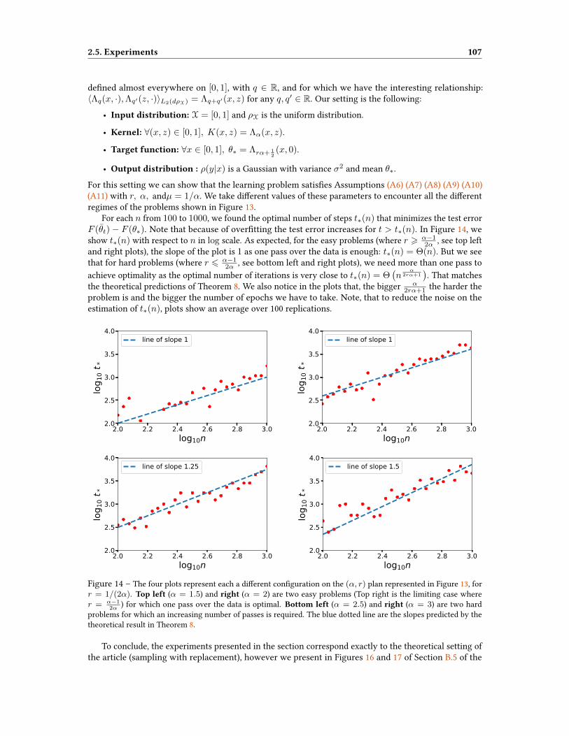
2.5. Experiments 107
dened almost everywhere on [0, 1], with q ∈ R, and for which we have the interesting relationship:〈Λq(x, ·),Λq′(z, ·)〉L2(dρX) = Λq+q′(x, z) for any q, q′ ∈ R. Our setting is the following:
• Input distribution: X = [0, 1] and ρX is the uniform distribution.
• Kernel: ∀(x, z) ∈ [0, 1], K(x, z) = Λα(x, z).
• Target function: ∀x ∈ [0, 1], θ∗ = Λrα+ 12(x, 0).
• Output distribution : ρ(y|x) is a Gaussian with variance σ2 and mean θ∗.
For this setting we can show that the learning problem satises Assumptions (A6) (A7) (A8) (A9) (A10)(A11) with r, α, andµ = 1/α. We take dierent values of these parameters to encounter all the dierentregimes of the problems shown in Figure 13.
For each n from 100 to 1000, we found the optimal number of steps t∗(n) that minimizes the test errorF (θt)− F (θ∗). Note that because of overtting the test error increases for t > t∗(n). In Figure 14, weshow t∗(n) with respect to n in log scale. As expected, for the easy problems (where r > α−1
2α , see top leftand right plots), the slope of the plot is 1 as one pass over the data is enough: t∗(n) = Θ(n). But we seethat for hard problems (where r 6 α−1
2α , see bottom left and right plots), we need more than one pass toachieve optimality as the optimal number of iterations is very close to t∗(n) = Θ
(n
α2rα+1
). That matches
the theoretical predictions of Theorem 8. We also notice in the plots that, the bigger α2rα+1 the harder the
problem is and the bigger the number of epochs we have to take. Note, that to reduce the noise on theestimation of t∗(n), plots show an average over 100 replications.
2.0 2.2 2.4 2.6 2.8 3.0log10n
2.0
2.5
3.0
3.5
4.0
log 1
0t *
line of slope 1
2.0 2.2 2.4 2.6 2.8 3.0log10n
2.0
2.5
3.0
3.5
4.0
log 1
0t *
line of slope 1
2.0 2.2 2.4 2.6 2.8 3.0log10n
2.0
2.5
3.0
3.5
4.0
log 1
0t *
line of slope 1.25
2.0 2.2 2.4 2.6 2.8 3.0log10n
2.0
2.5
3.0
3.5
4.0
log 1
0t *
line of slope 1.5
Figure 14 – The four plots represent each a dierent conguration on the (α, r) plan represented in Figure 13, forr = 1/(2α). Top left (α = 1.5) and right (α = 2) are two easy problems (Top right is the limiting case wherer = α−1
2α) for which one pass over the data is optimal. Bottom left (α = 2.5) and right (α = 3) are two hard
problems for which an increasing number of passes is required. The blue dotted line are the slopes predicted by thetheoretical result in Theorem 8.
To conclude, the experiments presented in the section correspond exactly to the theoretical setting ofthe article (sampling with replacement), however we present in Figures 16 and 17 of Section B.5 of the

2.6. Conclusion 108
Appendix results on the same datasets for two dierent ways of sampling the data: (a)without replacement:for which we select randomly the data points but never use twice the same point in one epoch, (b) cycles:for which we pick successively the data points in the same order. The obtained scalings relating numberof iterations or passes to number of observations are the same.
Linear model. To illustrate our result with some real data, we show how the optimal number of passesover the data increases with the number of samples. In Figure 15, we simply performed linear least-squaresregression on the MNIST dataset and plotted the optimal number of passes over the data that leads to thesmallest error on the test set. Evaluating α and r from Assumptions (A9) and (A10), we found α = 1.7and r = 0.18. As r = 0.18 6 α−1
2α ∼ 0.2, Theorem 8 indicates that this corresponds to a situation whereonly one pass on the data is not enough, conrming the behavior of Figure 15. This suggests that learningMNIST with linear regression is a hard problem.
1000 2000 3000 4000 5000 6000 7000 8000Number of samples
30
40
50
60
Optim
al num
ber o
f passes
Figure 15 – For the MNIST data set, we show the optimal number of passes over the data with respect to the numberof samples in the case of the linear regression.
2.6. Conclusion
In this paper, we have shown that for least-squares regression, in hard problems where single-passSGD is not statistically optimal (r < α−1
2α ), then multiple passes lead to statistical optimality with a numberof passes that somewhat surprisingly needs to grow with sample size, with a convergence rate which issuperior to previous analyses of stochastic gradient. Using a non-parametric estimation, we show thatunder certain conditions (2r > µ), we attain statistical optimality.
Our work could be extended in several ways: (a) our experiments suggest that cycling over the data andcycling with random reshuing perform similarly to sampling with replacement, it would be interesting tocombine our theoretical analysis with work aiming at analyzing other sampling schemes [Sha16, GOP15].(b) Mini-batches could be also considered with a potentially interesting eects compared to the streamingsetting. Also, (c) our analysis focuses on least-squares regression, an extension to all smooth loss functionswould widen its applicability. Moreover, (d) providing optimal ecient algorithms for the situation 2r < µis a clear open problem (for which the optimal rate is not known, even for non-ecient algorithms).Additionally, (e) in the context of classication, we could combine our analysis with [PVRB18] to study thepotential discrepancies between training and testing losses and errors when considering high-dimensionalmodels [ZBH+16]. More generally, (f) we could explore the eect of our analysis for methods based on theleast-squares estimator in the context of structured prediction [CRR16, OBLJ17, CBR18] and (non-linear)multitask learning [CRRP17]. Finally, (g) to reduce the computational complexity of the algorithm, whileretaining the (optimal) statistical guarantees, we could combine multi-pass stochastic gradient descent,

2.6. Conclusion 109
with approximation techniques like random features [RR08], extending the analysis of [CRR18] to themore general setting considered in this paper.
Acknowledgements
We acknowledge support from the European Research Council (grant SEQUOIA 724063). We alsothank Raphaël Berthier and Yann Labbé for their enlightening advices on this project.
?
? ?

B. Appendixof StatisticalOptimalityof
SGDonHardLearningProblemsthrough
Multiple Passes
The appendix in constructed as follows:
• We rst present in Section B.1 a new result for stochastic gradient recursions which generalizes thework of [BM13] and [DB16] to more general norms. This result could be used in other contexts.
• The proof technique for Theorem 8 is presented in Section B.2.
• In Section B.3 we give a proof of the various lemmas needed in the rst part of the proof of Theorem 8(deviation between SGD and batch gradient descent).
• In Section B.4 we provide new results for the analysis of batch gradient descent, which are adaptedto our new (A8), and instrumental in proving Theorem 8 in Section B.2.
• Finally, in Section B.5 we present experiments for dierent sampling techniques.
B.1. A general result for the SGD variance term
Independently of the problem studied in this paper, we consider i.i.d. observations (zt, ξt) ∈ H ×H aHilbert space, and the recursion started from µ0 = 0.
µt = (I − γzt ⊗ zt)µt−1 + γξt (76)
(this will applied with zt = Φ(xi(t))). This corresponds to the variance term of SGD. We denote by µt theaveraged iterate µt = 1
t
∑ti=1 µi.
The goal of the proposition below is to provide a bound on E[∥∥Hu/2µt
∥∥2]
for u ∈ [0, 1α + 1], where
H = E [zt ⊗ zt] is such that trH1/α is nite. Existing results only cover the case u = 1.Proposition 9 (A general result for the SGD variance term)
Let us consider the recursion in (76) started at µ0 = 0. Denote E [zt ⊗ zt] = H , assume that trH1/α isnite, E [ξt] = 0, E
[(zt ⊗ zt)2
]4 R2H , E [ξt ⊗ ξt] 4 σ2H and γR2 6 1/4, then for u ∈ [0, 1
α + 1]:
E[∥∥∥Hu/2µt
∥∥∥2]6 4σ2γ1−u γ
1/αtrH1/α
tu−1/α. (77)
B.1.1. Proof principle
We follow closely the proof technique of [BM13], and prove Proposition 9 by showing it rst for a“semi-stochastic” recursion, where zt ⊗ zt is replaced by its expectation (see Lemma 11). We will thencompare our general recursion to the semi-stochastic one.
110

B.1. A general result for the SGD variance term 111
B.1.2. Semi-stochastic recursion
Lemma 11 (Semi-stochastic SGD)
Let us consider the following recursion µt = (I − γH)µt−1 + γξt started at µ0 = 0. Assume thattrH1/α is nite, E [ξt] = 0, E [ξt ⊗ ξt] 4 σ2H and γH 4 I , then for u ∈ [0, 1
α + 1]:
E[∥∥∥Hu/2µt
∥∥∥2]6 σ2γ1−u γ1/αtrH1/αt1/α−u. (78)
Proof : For t > 1 and u ∈ [0, 1α
+ 1], using an explicit formula for µt and µt (see [BM13] for details), we get:
µt = (I − γH)µt−1 + γξt = (I − γH)t µ0 + γ
t∑k=1
(I − γH)t−k ξk
µt =1
t
t∑u=1
µu =γ
t
t∑u=1
u∑k=1
(I − γH)u−k ξk =1
t
t∑k=1
H−1(I − (I − γH)t−k+1
)ξk
E[∥∥∥Hu/2µt
∥∥∥2]
=1
t2E
t∑k=1
tr
[(I − (I − γH)t−k+1
)2
Hu−2ξk ⊗ ξk]
6σ2
t2
t∑k=1
tr
[(I − (I − γH)k
)2
Hu−1
]using E [ξt ⊗ ξt] 4 σ2H.
Now, let (λi)i∈N∗ be the non-increasing sequence of eigenvalues of the operator H . We obtain:
E[∥∥∥Hu/2µt
∥∥∥2]6σ2
t2
t∑k=1
∞∑i=1
(I − (I − γλi)k
)2
λu−1i .
We can now use a simple result9 that for any ρ ∈ [0, 1], k > 1 and u ∈ [0, 1α
+1], we have : (1− (1−ρ)k)2 6
(kρ)1−u+1/α, applied to ρ = γλi. We get, by comparing sums to integrals:
E[∥∥∥Hu/2µt
∥∥∥2]6σ2
t2
t∑k=1
∞∑i=1
(I − (I − γλi)k
)2
λu−1i
6σ2
t2
t∑k=1
∞∑i=1
(kγλi)1−u+1/αλu−1
i
6σ2
t2γ1−u+1/αtrH1/α
t∑k=1
k1−u+1/α
6σ2
t2γ1−u+1/αtrH1/α
∫ t
1
y1−u+1/αdy
6σ2
t2γ1−u γ1/αtrH1/α t2−u+1/α
2− u+ 1/α
6 σ2γ1−u γ1/αtrH1/αt1/α−u,
which shows the desired result.
9Indeed, adapting a similar result from [BM13], on the one hand, 1− (1− ρ)k 6 1 implying that (1− (1− ρ)k)1−1/α+u 6 1.On the other hand, 1− (1− γx)k 6 γkx implying that (1− (1− ρ)k)1+1/α−u 6 (kρ)1+1/α−u. Thus by multiplying the twowe get (1− (1− ρ)k)2 6 (kρ)1−u+1/α.

B.1. A general result for the SGD variance term 112
B.1.3. Relating the semi-stochastic recursion to the main recursion
Then, to relate the semi-stochastic recursion with the true one, we use an expansion in the powers ofγ using recursively the perturbation idea from [AMP00].
For r > 0, we dene the sequence (µrt )t∈N, for t > 1,
µrt = (I − γH)µrt−1 + γΞrt , with Ξrt =
(H − zt ⊗ zt)µr−1
t−1 if r > 1
Ξ0t = ξt
. (79)
We will show that µt '∑∞i=0 µ
it. To do so, notice that for r > 0, µt −
∑ri=0 µ
it follows the recursion:
µt −r∑i=0
µit = (I − zt ⊗ zt)
(µt−1 −
r∑i=0
µit−1
)+ γΞr+1
t , (80)
so that by bounding the covariance operator we can apply a classical SGD result. This is the purpose ofthe following lemma.Lemma 12 (Bound on covariance operator)
For any r > 0, we have the following inequalities:
E [Ξrt ⊗ Ξrt ] 4 γrR2rσ2H and E [µrt ⊗ µrt ] 4 γr+1R2rσ2I. (81)
Proof : We propose a proof by induction on r. For r = 0, and t > 0, E[Ξ0t ⊗ Ξ0
t
]= E [ξt ⊗ ξt] 4 σ2H by
assumption. Moreover,
E[µ0t ⊗ µ0
t
]= γ2
t−1∑k=1
(I − γH)t−kE[Ξ0t ⊗ Ξ0
t
](I − γH)t−k 4 γ2σ2
t−1∑k=1
(I − γH)2(t−k)H 4 γσ2I.
Then, for r > 1,
E[Ξr+1t ⊗ Ξr+1
t
]4 E[(H − zt ⊗ zt)µrt−1 ⊗ µrt−1(H − zt ⊗ zt)]= E[(H − zt ⊗ zt)E[µrt−1 ⊗ µrt−1](H − zt ⊗ zt)]
4 γr+1R2rσ2E[(H − zt ⊗ zt)2]
4 γr+1R2r+2σ2H.
And,
E[µr+1t ⊗ µr+1
t
]= γ2
t−1∑k=1
(I − γH)t−kE[Ξr+1t ⊗ Ξr+1
t
](I − γH)t−k
4 γr+3R2r+2σ2t−1∑k=1
(I − γH)2(t−k)H 4 γr+2R2r+2σ2I,
which thus shows the lemma by induction.
To bound µt −∑ri=0 µ
it, we prove a very loose result for the average iterate, that will be sucient for our
purpose.Lemma 13 (Bounding SGD recursion)
Let us consider the following recursion µt = (I − γzt ⊗ zt)µt−1 +γξt starting at µ0 = 0. Assume that

B.1. A general result for the SGD variance term 113
E[zt ⊗ zt] = H , E [ξt] = 0, ‖xt‖2 6 R2, E [ξt ⊗ ξt] 4 σ2H and γR2 < I , then for u ∈ [0, 1α + 1]:
E[∥∥∥Hu/2µt
∥∥∥2]6 σ2γ2RutrH t. (82)
Proof : Let us dene the operators for j 6 i : M ij = (I − γzi(i) ⊗ zi(i)) · · · (I − γzi(j) ⊗ zi(j)) and M i
i+1 = I .Since µ0 = 0, note that we have we have, µi = γ
∑ik=1 M
ik+1ξk . Hence, for i > 1,
E∥∥∥Hu/2µi
∥∥∥2
= γ2E∑k,j
〈M ij+1ξj , H
uM ik+1ξk〉
= γ2Ei∑
k=1
〈M ik+1ξk, H
uM ik+1ξk〉
= γ2tr
(E
[i∑
k=1
M ik+1∗HuM i
k+1ξk ⊗ ξk
])6 σ2γ2E
[i∑
k=1
tr(M ik+1∗HuM i
k+1H)]
6 σ2γ2Rui trH,
because tr(M ik+1∗HuM i
k+1H)6 RutrH . Then,
E∥∥∥Hu/2µt
∥∥∥2
=1
t2
∑i,j
〈Hu/2µi, Hu/2µj〉
61
t2E
(t∑i=1
∥∥∥Hu/2µi
∥∥∥)2
61
t
t∑i=1
E∥∥∥Hu/2µi
∥∥∥2
6 σ2γ2RutrH t,
which nishes the proof of Lemma 13.
B.1.4. Final steps of the proof
We have now all the material to conclude. Indeed by the triangular inequality:
(E∥∥∥Hu/2µt
∥∥∥2)1/2
6r∑i=1
E∥∥∥Hu/2µit
∥∥∥2
︸ ︷︷ ︸Lemma 11
1/2
+
E
∥∥∥∥∥Hu/2
(µt −
r∑i=1
µit
)∥∥∥∥∥2
︸ ︷︷ ︸Lemma 13
1/2
.
With Lemma 12, we have all the bounds on the covariance of the noise, so that:(E∥∥∥Hu/2µt
∥∥∥2)1/2
6r∑i=1
(γiR2iσ2γ1−u γ1/αtrH1/αt1/α−u
)1/2
+(γr+2R2r+utrH t
)1/26 (σ2γ1−u γ1/αtrH1/αt1/α−u)1/2
r∑i=1
(γR2
)i/2+(γr+2R2r+utrH t
)1/2.
Now we make r go to innity and we obtain:(E∥∥∥Hu/2µt
∥∥∥2)1/2
6 (σ2γ1−u γ1/αtrH1/αt1/α−u)1/2 1
1−√γR2
+(γr+2R2r+utrH t
)1/2︸ ︷︷ ︸−→r→∞
0

B.2. Proof sketch for Theorem 8 114
Hence with γR2 6 1/4,
E∥∥∥Hu/2µt
∥∥∥2
6 4σ2γ1−u γ1/αtrH1/αt1/α−u,
which nishes to prove Proposition 9.
B.2. Proof sketch for Theorem 8
We consider the batch gradient descent recursion, started from η0 = 0, with the same step-size:
ηt = ηt−1 +γ
n
n∑i=1
(yi − 〈ηt−1,Φ(xi)〉H
)Φ(xi),
as well as its averaged version ηt = 1t
∑ti=0 ηi. We obtain a recursion for θt − ηt, with the initialization
θ0 − η0 = 0, as follows:
θt − ηt =[I − Φ(xi(u))⊗H Φ(xi(u))
](θt−1 − ηt−1) + γξ1
t + γξ2t ,
with ξ1t = yi(u)Φ(xi(u)) − 1
n
∑ni=1 yiΦ(xi) and ξ2
t =[Φ(xi(u)) ⊗H Φ(xi(u)) − 1
n
∑ni=1 Φ(xi) ⊗H
Φ(xi)]ηt−1. We decompose the performance F (θt) in two parts, one analyzing the performance of batch
gradient descent, one analyzing the deviation θt − ηt, using
EF (θt)− F (θ∗) 6 2E[‖Σ1/2(θt − ηt)‖2H
]+ 2[EF (ηt)− F (θ∗)
].
We denote by Σn = 1n
∑ni=1 Φ(xi)⊗ Φ(xi) the empirical second-order moment.
Deviation θt − ηt. Denoting by G the σ-eld generated by the data and by Ft the σ-eld generated byi(1), . . . , i(t), then, we have E(ξ1
t |G,Ft−1) = E(ξ2t |G,Ft−1) = 0, thus we can apply results for averaged
SGD (see Proposition 9 of the Appendix) to get the following lemma.Lemma 14
For any t > 1, ifE[(ξ1t+ξ2
t )⊗H(ξ1t+ξ2
t )|G]4 τ2Σn, and 4γR2 = 1, under Assumptions (A6), (A7), (A9),
E[‖Σ1/2
n (θt − ηt)‖2H|G]6
8τ2γ1/αtr Σ1/αn
t1−1/α. (83)
In order to obtain the bound, we need to bound τ2 (which is dependent on G) and go from a bound withthe empirical covariance matrix Σn to bounds with the population covariance matrix Σ.
We have
E[ξ1t ⊗H ξ1
t |G]4H E
[y2i(u)Φ(xi(u))⊗H Φ(xi(u))|G
]4H ‖y‖2∞Σn 4H (σ + sup
x∈X〈θ∗,Φ(x)〉H)2Σn
E[ξ2t ⊗ ξ2
t |G]4H E
[〈ηt−1,Φ(xi(u))〉2Φ(xi(u))⊗H Φ(xi(u))|G
]4H sup
t∈0,...,T−1supx∈X〈ηt,Φ(x)〉H)2Σn
Therefore τ2 = 2M2 + 2 supt∈0,...,T−1 supx∈X〈ηt,Φ(x)〉2H or using Assumption (A8) τ2 = 2M2 +
2 supt∈0,...,T−1R2µκ2
µ‖Σ1/2−µ/2ηt‖2H.In the proof, we rely on an event (that depend on G) where Σn is close to Σ. This leads to the the
following Lemma that bounds the deviation θt − ηt.

B.3. Bounding the deviation between SGD and batch gradient descent 115
Lemma 15
For any t > 1, 4γR2 = 1, under Assumptions (A6), (A7), (A9),
E[‖Σ1/2(θt − ηt)‖2H
]6 16τ2
∞
[R−2/αtr Σ1/αt1/α
(1
t+
(4
µ
log n
n
)1/µ)
+ 1
]. (84)
We make the following remark on the bound.Remark 5
Note that as dened in the proof τ∞ may diverge in some cases as
τ2∞ =
O(1) when µ 6 2r,
O(nµ−2r) when 2r 6 µ 6 2r + 1/α,
O(n1−2r/µ) when µ > 2r + 1/α,
with O(·) are dened explicitly in the proof.
Convergence of batch gradient descent. The main result is summed up in the following lemma, witht = O(n1/µ) and t > n.Lemma 16
Let t > 1, under Assumptions (A6), (A7), (A8), (A9), (A10), (A11), when, with 4γR2 = 1,
t =
Θ(nα/(2rα+1)) 2rα+ 1 > µα
Θ(n1/µ (log n)1µ ) 2rα+ 1 6 µα.
(85)
then,
EF (ηt)− F (θ∗) 6
O(n−2rα/(2rα+1)) 2rα+ 1 > µα
O(n−2r/µ) 2rα+ 1 6 µα(86)
with O(·) are dened explicitly in the proof.
Remark 6
In all cases, we can notice that the speed of convergence of Lemma 16 are slower that the ones in Lemma15, hence, the convergence of the gradient descent controls the rates of convergence of the algorithm.
B.3. Bounding the deviation between SGD and batch
gradient descent
In this section, following the proof sketch from Section B.2, we provide a bound on the deviationθt − ηt. In all the following let us denote µt = θt − ηt that deviation between the stochastic gradientdescent recursion and the batch gradient descent recursion.

B.3. Bounding the deviation between SGD and batch gradient descent 116
B.3.1. Proof of Lemma 15
We need to (a) go from Σn to Σ in the result of Lemma 14 and (b) to have a bound on τ . To prove thisresult we are going to need the two following lemmas:Lemma 17
Let λ > 0, δ ∈ (0, 1]. Under Assumption (A8), when n > 11(1 + κ2µR
2µγµtµ) log 8R2
λδ , the followingholds with probability 1− δ, ∥∥∥(Σ + λI)1/2(Σn + λI)−1/2
∥∥∥2
6 2. (87)
Proof : This Lemma is proven and stated lately in Lemma 24 in Section B.4.3. We recalled it here for the sake ofclarity.
Lemma 18
Let λ > 0, δ ∈ (0, 1]. Under Assumption (A8), for t = O(
1n1/µ
)then the following holds with probability
1− δ,
τ2 6 τ2∞ and τ2
∞ =
O(1), when µ 6 2r,
O(nµ−2r
), when 2r 6 µ 6 2r + 1/α,
O(n1−2r/µ
)when µ > 2r + 1/α,
(88)
where the O(·)-notation depend only on the parameters of the problem (and is independent of n and t).
Proof : This Lemma is a direct implication of Corollary 6 in Section B.4.3. We recalled it here for the sake ofclarity.
Note that we can take λδn =(
log nδ
n
)1/µ
so that Lemma 17 result holds. Now we are ready to prove Lemma15.Proof of Lemma 15 : LetAδa be the set for which inequality (87) holds and letBδb be the set for which inequality
(88) holds. Note that P(Acδa) = δa and P(Bcδb) = δb. We use the following decomposition:
E∥∥∥Σ1/2µt
∥∥∥2
6 E[∥∥∥Σ1/2µt
∥∥∥2
1Aδa∩Bδb
]+ E
[∥∥∥Σ1/2µt
∥∥∥2
1Acδa
]+ E
[∥∥∥Σ1/2µt
∥∥∥2
1Bcδb
].
First, let us bound roughly ‖µt‖2.First, for i > 1, ‖µi‖2 6 γ2
(∑ti=1 ‖ξ
1i ‖+ ‖ξ2
i ‖)2
6 16R2γ2τ2t2, so that ‖µt‖2 6 1t
∑ti=1 ‖µi‖
2 616R2γ2τ2t2. We can bound similarly τ2 6 4M2γ2R4t2, so that ‖µt‖2 6 64R2M2γ4t4. Thus, for thesecond term:
E[∥∥∥Σ1/2µt
∥∥∥2
1Acδa
]6 64R8M2γ4t4E1Ac
δa6 64R8M2γ4t4δa,
and for the third term:
E[∥∥∥Σ1/2µt
∥∥∥2
1Bcδb
]6 64R8M2γ4t4E1Bc
δb6 64R8M2γ4t4δb.
B.4. Convergence of batch gradient descent 117
And on for the rst term,
E[∥∥∥Σ1/2µt
∥∥∥2
1Aδa∩Bδb
]6 E
[∥∥∥Σ1/2(Σ + λδnI)−1/2∥∥∥2 ∥∥∥(Σ + λδnI)1/2(Σn + λδnI)−1/2
∥∥∥2
∥∥∥(Σn + λδnI)1/2µt
∥∥∥2
1Aδa∩Bδb | G]
6 2E[∥∥∥(Σn + λδnI)1/2µt
∥∥∥2
| G]
= 2E[∥∥∥Σ1/2
n µt
∥∥∥2
| G]
+ 2λδnE[‖µt‖2 | G
]6 16τ2
∞
γ1/αE[tr Σ
1/αn
]t1−1/α
+ 8λδnτ2∞ γ1/αE
[tr Σ1/α
n
]t1/α,
using Proposition 9 twice with u = 1 for the left term and u = 1 for the right one.As x→ x1/α is a concave function, we can apply Jensen’s inequality to have :
E[tr(Σ1/α
n )]6 trΣ1/α,
so that:
E[∥∥∥Σ1/2µt
∥∥∥2
1Aδa∩Bδb
]6 16τ2
∞γ1/αtr Σ1/α
t1−1/α+ 8λδnτ
2∞γ γ
1/αtr Σ1/αt1/α
6 16τ2∞γ
1/αtr Σ1/αt1/α(
1
t+ λδn
).
Now, we take δa = δb =τ2∞
4M2R8γ4t4and this concludes the proof of Lemma 15, with the bound:
E∥∥∥Σ1/2µt
∥∥∥2
6 16τ2∞γ
1/αtr Σ1/αt1/α(
1
t+(2 + 2 logM + 4 log(γR2) + 4 log t
n
)1/µ).
B.4. Convergence of batch gradient descent
In this section we prove the convergence of averaged batch gradient descent to the target function. Inparticular, since the proof technique is valid for the wider class of algorithms known as spectral lters[GRO+08, LRRC18], we will do the proof for a generic spectral lter (in Lemma 19, Sect. B.4.1 we provethat averaged batch gradient descent is a spectral lter).
In Section B.4.1 we provide the required notation and additional denitions. In Section B.4.2, inparticular in Theorem B.4.2 we perform an analytical decomposition of the excess risk of the averagedbatch gradient descent, in terms of basic quantities that will be controlled in expectation (or probability)in the next sections. In Section B.4.3 the various quantites obtained by the analytical decompositionare controlled, in particular, Corollary 6 controls the L∞ norm of the averaged batch gradient descentalgorithm. Finally in Section B.4.4, the main result, Theorem 10 controlling in expectation of the excessrisk of the averaged batch gradient descent estimator is provided. In Corollary 7, a version of the result ofTheorem 10 is given, with explicit rates for the regularization parameters and of the excess risk.
B.4.1. Notations
In this subsection, we study the convergence of batch gradient descent. For the sake of claritywe consider the RKHS framework (which includes the nite-dimensional case). We will thus considerelements of H that are naturally embedded in L2(dρX) by the operator S from H to L2(dρX) and such

B.4. Convergence of batch gradient descent 118
that: (Sg)(x) = 〈g,Kx〉, where we have Φ(x) = Kx = K(·, x) where K : X → X → R is the kernel.We recall the recursion for ηt in the case of an RKHS feature space with kernel K :
ηt = ηt−1 +γ
n
n∑i=1
(yi − 〈ηt−1,Kxi〉H
)Kxi ,
Let us begin with some notations. In the following we will often use the letter g to denote vectors of H,hence, Sg will denote functions of L2(dρX). We also dene the following operators (we may also usetheir adjoints, denoted with a ∗):
• The operator Sn from H to Rn, Sng = 1√n
(g(x1), . . . g(xn)).
• The operators from H to H, Σ and Σn, dened respectively as Σ = E [Kx ⊗Kx] =∫XKx⊗KxdρX
and Σn = 1n
∑ni=1Kxi ⊗Kxi . Note that Σ is the covariance operator.
• The operator L : L2(dρX)→ L2(dρX) is dened by
(Lf)(x) =
∫X
K(x, z)f(z)dρX(x), ∀f ∈ L2(dρX).
Moreover denote by N(λ) the so called eective dimension of the learning problem, that is dened as
N(λ) = tr(L(L + λI)−1),
for λ > 0. Recall that by Assumption (A9), there exists α > 1 and Q > 0 such that
N(λ) 6 Qλ−1/α, ∀λ > 0.
We can take Q = trΣ1/α.
• P : L2(dρX)→ L2(dρX) projection operator on H for the L2(dρX) norm s.t. ranP = ranS.
Denote by fρ the function so that fρ(x) = E[y|x] ∈ L2(dρX) the minimizer of the expected risk, denedby F (f) =
∫X×R(f(x)− y)2dρ(x, y).
Remark 7 (On Assumption (A10))With the notation above, we express assumption (A10), more formally, w.r.t. Hilbert spaces with innitedimensions, as follows. There exists r ∈ [0, 1] and φ ∈ L2(dρX), such that
Pfρ = Lrφ.
(A11) Let q ∈ [1,∞] be such that ‖fρ − Pfρ‖L2q(X,ρX) <∞.
The assumption above is always true for q = 1, moreover when the kernel is universal it is trueeven for q = ∞. Moreover if r > 1/2 then it is true for q = ∞. Note that we make the calculation inthis Appendix for a general q ∈ [1,∞], but we presented the results for q =∞ in the main paper. Thefollowing proposition relates the excess risk to a certain norm.Proposition 10
When g ∈ H,F (g)− inf
g∈HF (g) = ‖Sg − Pfρ‖2L2(dρX).

B.4. Convergence of batch gradient descent 119
We introduce the following function gλ ∈ H that will be useful in the rest of the paper gλ =(Σ + λI)−1S∗fρ.
We introduce the estimators of the form, for λ > 0,
gλ = qλ(Σn)S∗ny,
where qλ : R+ → R+ is a function called lter, that essentially approximates x−1 with the approximationcontrolled by λ. Denote moreover with rλ the function rλ(x) = 1 − xqλ(x). The following denitionprecises the form of the lters we want to analyze. We then prove in Lemma 19 that our estimatorcorresponds to such a lter.Denition 2 (Spectral lters)
Let qλ : R+ → R+ be a function parametrized by λ > 0. qλ is called a lter when there exists cq > 0for which
λqλ(x) 6 cq, rλ(x)xu 6 cqλu, ∀x > 0, λ > 0, u ∈ [0, 1].
We now justify that we study estimators of the form gλ = qλ(Σn)S∗ny with the following lemma. Indeed,we show that the average of batch gradient descent can be represented as a lter estimator, gλ, forλ = 1/(γt).Lemma 19
For t > 1, λ = 1/(γt), ηt = gλ, with respect to the lter, qη(x) =(
1− 1−(1−γx)t
γtx
)1x .
Proof : Indeed, for t > 1,
ηt = ηt−1 +γ
n
n∑i=1
(yi − 〈ηt−1,Kxi〉H
)Kxi
= ηt−1 + γ(S∗ny − Σnηt−1)
= (I − γΣn)ηt−1 + γS∗ny
= γ
t−1∑k=0
(I − γΣn)kS∗ny =[I − (I − γΣn)t
]Σ−1n S∗ny,
leading to
ηt =1
t
t∑i=0
ηi = qη(
Σn)S∗ny.
Now, we prove that q has the properties of a lter. First, for t > 1, 1γtqη(x) =
(1− 1−(1−γx)t
γtx
)1γtx
is a
decreasing function so that 1γtqη(x) 6 1
γtqη(0) 6 1. Second for u ∈ [0, 1], xu(1− xqη(x)) = 1−(1−γx)t
γtxxu.
As used in Section B.1.2, 1− (1− γx)t 6 (γtx)1−u, so that, rη(x)xu 6 (γtx)1−u
γtxxu = 1
(γt)u, this concludes
the proof that qη is indeed a lter.
B.4.2. Analytical decomposition
Lemma 20
Let λ > 0 and s ∈ (0, 1/2]. Under Assumption (A10) (see Rem. 7), the following holds
‖L−sS(gλ − gλ)‖L2(dρX) 6 2λ−sβ2cq‖Σ−1/2λ (S∗ny − Σngλ)‖H + 2βcq‖φ‖L2(dρX)λ
r−s,
where β := ‖Σ1/2λ Σ
−1/2nλ ‖.
B.4. Convergence of batch gradient descent 120
Proof : By Prop. 10, we can characterize the excess risk of gλ in terms of theL2(dρX) squared norm of Sgλ−Pfρ.In this paper, simplifying the analysis of [LRRC18], we perform the following decomposition
L−sS(gλ − gλ) = L
−sSgλ − L−sSqλ(Σn)Σngλ
+ L−sSqλ(Σn)Σngλ − L
−sSgλ.
Upper bound for the rst term. By using the denition of gλ and multiplying and dividing by Σ1/2λ , we
have that
L−sSgλ − L
−sSqλ(Σn)Σngλ = L−sSqλ(Σn)(S∗ny − Σngλ)
= L−sSqλ(Σn)Σ
1/2λ Σ
−1/2λ (S∗ny − Σngλ),
from which
‖L−sS(gλ − qλ(Σn)Σngλ)‖L2(dρX) 6 ‖L−sSqλ(Σn)Σ1/2λ ‖ ‖Σ
−1/2λ (S∗ny − Σngλ)‖H.
Upper bound for the second term. By denition of rλ(x) = 1− xqλ(x) and gλ = Σ−1λ S∗fρ,
L−sSqλ(Σn)Σngλ − L
−sSgλ = L−sS(qλ(Σn)Σn − I)gλ
= −L−sSrλ(Σn) Σ−(1/2−r)λ Σ
−1/2−rλ S∗Lr φ,
where in the last step we used the fact that S∗fρ = S∗Pfρ = S∗Lrφ, by Asm. (A10) (see Rem. 7). Then
‖L−sS(qλ(Σn)Σn − I)gλ)‖L2(dρX) 6 ‖L−sSrλ(Σn)‖‖Σ−(1/2−r)λ ‖‖Σ−1/2−r
λ S∗Lr‖‖φ‖L2(dρX)
6 λ−(1/2−r)‖L−sSrλ(Σn)‖‖φ‖L2(dρX),
where the last step is due to the fact that ‖Σ−(1/2−r)λ ‖ 6 λ−(1/2−r) and that S∗L2rS = S∗(SS∗)2rS =
(S∗S)2rS∗S = Σ1+2r from which
‖Σ−1/2−rλ S∗Lr‖2 = ‖Σ−1/2−r
λ S∗L2rSΣ−1/2−rλ ‖ = ‖Σ−1/2−r
λ Σ1+2rΣ−1/2−rλ ‖ 6 1. (89)
Additional decompositions. We further bound ‖L−sSrλ(Σn)‖ and ‖L−sSqλ(Σn)Σ1/2λ ‖. For the rst, by
the identity L−sSrλ(Σn) = L−sSΣ−1/2nλ Σ
1/2nλ rλ(Σn), we have
‖L−sSrλ(Σn)‖ = ‖L−sSΣ−1/2nλ ‖‖Σ1/2
nλ rλ(Σn)‖,
where‖Σ1/2
nλ rλ(Σn)‖ = supσ∈σ(Σn)
(σ + λ)1/2rλ(σ) 6 supσ>0
(σ + λ)1/2rλ(σ) 6 2cqλ1/2.
Similarly, by using the identity
L−sSqλ(Σn)Σ
1/2λ = L
−sSΣ−1/2nλ Σ
1/2nλ qλ(Σn)Σ
1/2nλ Σ
−1/2nλ Σ
1/2λ ,
we have‖L−sSqλ(Σn)Σ
1/2λ ‖ = ‖L−sSΣ
−1/2nλ ‖ ‖Σ1/2
nλ qλ(Σn)Σ1/2nλ ‖ ‖Σ
−1/2nλ Σ
1/2λ ‖.
Finally note that‖L−sSΣ
−1/2nλ ‖ 6 ‖L−sSΣ
−1/2+sλ ‖‖Σ−sλ ‖‖Σ
1/2λ Σ
−1/2nλ ‖,
and ‖L−sSΣ−1/2+sλ ‖ 6 1, ‖Σ−sλ ‖ 6 λ−s, and moreover
‖Σ1/2nλ qλ(Σn)Σ
1/2nλ ‖ = sup
σ∈σ(Σn)
(σ + λ)qλ(σ) 6 supσ>0
(σ + λ)qλ(σ) 6 2cq,
so, in conclusion
‖L−sSrλ(Σn)‖ 6 2cqλ1/2−sβ, ‖L−sSqλ(Σn)Σ
1/2λ ‖ 6 2cqλ
−sβ2.
The nal result is obtained by gathering the upper bounds for the three terms above and the additional termsof this last section.
B.4. Convergence of batch gradient descent 121
Lemma 21
Let λ > 0 and s ∈ (0,min(r, 1/2)]. Under Assumption (A10) (see Rem. 7), the following holds
‖L−s(Sgλ − Pfρ)‖L2(dρX) 6 λr−s‖φ‖L2(dρX).
Proof : Since SΣ−1λ S∗ = LL−1
λ = I − λL−1λ , we have
L−s(Sgλ − Pfρ) = L
−s(SΣ−1λ S∗fρ − Pfρ) = L
−s(SΣ−1λ S∗Pfρ − Pfρ)
= L−s(SΣ−1
λ S∗ − I)Pfρ = L−s(SΣ−1
λ S∗ − I)Lr φ
= −λL−sL−1λ Lrφ = −λr−s λ1−r+s
L−(1−r+s)λ L
−(r−s)λ L
r−s φ,
from which
‖L−s(Sgλ − Pfρ)‖L2(dρX) 6 λr−s‖λ1−r+sL−(1−r+s)λ ‖‖L−(r−s)
λ Lr−s‖ ‖φ‖L2(dρX)
6 λr−s‖φ‖L2(dρX).
Theorem 9
Let λ > 0 and s ∈ (0,min(r, 1/2)]. Under Assumption (A10) (see Rem. 7), the following holds
‖L−s(Sgλ − Pfρ)‖L2(dρX) 6 2λ−sβ2cq‖Σ−1/2λ (S∗ny − Σngλ)‖H +
(1 + β2cq‖φ‖L2(dρX)
)λr−s
where β := ‖Σ1/2λ Σ
−1/2nλ ‖.
Proof : By Prop. 10, we can characterize the excess risk of gλ in terms of theL2(dρX) squared norm of Sgλ−Pfρ.In this paper, simplifying the analysis of [LRRC18], we perform the following decomposition
L−s(Sgλ − Pfρ) = L
−sSgλ − L−sSgλ
+ L−s(Sgλ − Pfρ).
The rst term is bounded by Lemma 20, the second is bounded by Lemma 21.
B.4.3. Probabilistic bounds
In this section denote by N∞(λ), the quantity
N∞(λ) = supx∈S‖Σ−1/2
λ Kx‖2H,
where S ⊆ X is the support of the probability measure ρX.Lemma 22
Under Asm. (A8), we have that for any g ∈ H
supx∈supp(ρX)
|g(x)| 6 κµRµ‖Σ1/2(1−µ)g‖H = κµR
µ‖L−µ/2Sg‖L2(dρX).
Proof : Note that, Asm. (A8) is equivalent to
‖Σ−1/2(1−µ)Kx‖ 6 κµRµ,

B.4. Convergence of batch gradient descent 122
for all x in the support of ρX. Then we have, for any x in the support of ρX,
|g(x)| = 〈g,Kx〉H =⟨
Σ1/2(1−µ)g,Σ−1/2(1−µ)Kx
⟩H
6 ‖Σ1/2(1−µ)g‖H‖Σ−1/2(1−µ)Kx‖ 6 κµRµ‖Σ1/2(1−µ)g‖H.
Now note that, since Σ1−µ = S∗L−µS, we have
‖Σ1/2(1−µ)g‖2H =⟨g,Σ1−µg
⟩H
=⟨L−µ/2Sg,L−µ/2Sg
⟩L2(dρX)
.
Lemma 23
Under Assumption (A8), we haveN∞(λ) 6 κ2
µR2µλ−µ.
Proof : First denote with fλ,u ∈ H the function Σ−1/2λ u for any u ∈ H and λ > 0. Note that
‖fλ,u‖H = ‖Σ−1/2λ u‖H 6 ‖Σ−1/2
λ ‖‖u‖H 6 λ−1/2‖u‖H.
Moreover, since for any g ∈ H the identity ‖g‖L2(dρX) = ‖Sg‖H, we have
‖fλ,u‖L2(dρX) = ‖SΣ−1/2λ u‖H 6 ‖SΣ
−1/2λ ‖‖u‖H 6 ‖u‖H.
Now denote with B(H) the unit ball in H, by applying Asm. (A8) to fλ,u we have that
N∞(λ) = supx∈S‖Σ−1/2
λ Kx‖2 = supx∈S,u∈B(H)
⟨u,Σ
−1/2λ Kx
⟩2
H
= supx∈S,u∈B(H)
〈fλ,u,Kx〉2H = supu∈B(H)
supx∈S|fλ,u(x)|2
6 κ2µR
2µ supu∈B(H)
‖fλ,u‖2µH ‖fλ,u‖2−2µL2(dρX)
6 κ2µR
2µλ−µ supu∈B(H)
‖u‖2H 6 κ2µR
2µλ−µ.
Lemma 24
Let λ > 0, δ ∈ (0, 1] and n ∈ N. Under Assumption (A8), we have that, when
n > 11(1 + κ2µR
2µλ−µ) log8R2
λδ,
then the following holds with probability 1− δ,
‖Σ1/2λ Σ
−1/2nλ ‖2 6 2.
Proof : This result is a renement of the one in [RCR13] and is based on non-commutative Bernstein inequalitiesfor random matrices [Tro12a]. By Prop. 8 in [RR17], we have that
‖Σ1/2λ Σ
−1/2nλ ‖2 6 (1− t)−1, t := ‖Σ−1/2
λ (Σ− Σn)Σ−1/2λ ‖.
When 0 < λ 6 ‖Σ‖, by Prop. 6 of [RR17] (see also [RCR17] Lemma 9 for more rened constants), we havethat the following holds with probability at least 1− δ,
t 62η(1 + N∞(λ))
3n+
√2ηN∞(λ)
n,
with η = log 8R2
λδ. Finally, by selecting n > 11(1 + κ2
µR2µλ−µ)η, we have that t 6 1/2 and so
‖Σ1/2λ Σ
−1/2nλ ‖2 6 (1− t)−1 6 2, with probability 1− δ.

B.4. Convergence of batch gradient descent 123
To conclude note that when λ > ‖Σ‖, we have
‖Σ1/2λ Σ
−1/2nλ ‖2 6 ‖Σ + λI‖‖(Σn + λI)−1‖ 6 ‖Σ‖+ λ
λ= 1 +
‖Σ‖λ
6 2.
Lemma 25
Under Assumption (A8), (A9), (A10) (see Rem. 7), (A11) we have
1. Let λ > 0, n ∈ N, the following holds
E[‖Σ−1/2λ (S∗ny − Σngλ)‖2H] 6 ‖φ‖2L2(dρX)λ
2r +2κ2
µR2µλ−(µ−2r)
n+
4κ2µR
2µAQλ−q+µαqα+α
n,
where A := ‖fρ − Pfρ‖2−2/(q+1)L2q(X,ρX) .
2. Let δ ∈ (0, 1], under the same assumptions, the following holds with probability at least 1− δ
‖Σ−1/2λ (S∗ny − Σngλ)‖H 6 c0λ
r +4(c1λ
−µ2 + c2λ−r−µ) log 2
δ
n
+
√16κ2
µR2µ(λ−(µ−2r) + 2AQλ−
q+µαqα+α ) log 2
δ
n,
with c0 = ‖φ‖L2(dρX), c1 = κµRµM + κ2
µR2µ(2R)2r−µ‖φ‖L2(dρX), c2 = κ2
µR2µ‖φ‖L2(dρX)
Proof : First denote with ζi the random variable
ζi = (yi − gλ(xi))Σ−1/2λ Kxi .
In particular note that, by using the denitions of Sn, y and Σn, we have
Σ−1/2λ (S∗ny − Σngλ) = Σ
−1/2λ (
1
n
n∑i=1
Kxiyi −1
n(Kxi ⊗Kxi)gλ) =
1
n
n∑i=1
ζi.
I So, by noting that ζi are independent and identically distributed, we have
E[‖Σ−1/2λ (S∗ny − Σngλ)‖2H] = E[‖ 1
n
n∑i=1
ζi‖2H] =1
n2
n∑i,j=1
E[〈ζi, ζj〉H]
=1
nE[‖ζ1‖2H] +
n− 1
n‖E[ζ1]‖2H.
Now note that
E[ζ1] = Σ−1/2λ (E[Kx1y1]− E[Kx1 ⊗Kx1 ]gλ) = Σ
−1/2λ (S∗fρ − Σgλ).
In particular, by the fact that S∗fρ = Pfρ, Pfρ = Lrφ and Σgλ = ΣΣ−1λ S∗fρ and ΣΣ−1
λ = I − λΣ−1λ , we
haveΣ−1/2λ (S∗fρ − Σgλ) = λΣ
−3/2λ S∗fρ = λr λ1−rΣ
−(1−r)λ Σ
−1/2−rλ S∗Lr φ.
So, since ‖Σ−1/2−rλ S∗Lr‖ 6 1, as proven in Eq. 89, then
‖E[ζ1]‖H 6 λr‖λ1−rΣ−(1−r)λ ‖ ‖Σ−1/2−r
λ S∗Lr‖ ‖φ‖L2(dρX) 6 λr‖φ‖L2(dρX) := Z.
Morever
E[‖ζ1‖2H] = E[‖Σ−1/2λ Kx1‖
2H(y1 − gλ(x1))2] = Ex1Ey1|x1 [‖Σ−1/2
λ Kx1‖2H(y1 − gλ(x1))2]
= Ex1 [‖Σ−1/2λ Kx1‖
2H(fρ(x1)− gλ(x1))2].

B.4. Convergence of batch gradient descent 124
Moreover we have
E[‖ζ1‖2H] = Ex[‖Σ−1/2λ Kx‖2H(fρ(x)− gλ(x))2]
= Ex[‖Σ−1/2λ Kx‖2H((fρ(x)− (Pfρ)(x)) + ((Pfρ)(x)− gλ(x)))2]
6 2Ex[‖Σ−1/2λ Kx‖2H(fρ(x)− (Pfρ)(x))2] + 2Ex[‖Σ−1/2
λ Kx‖2H((Pfρ)(x)− gλ(x))2].
Now since E[AB] 6 (ess supA)E[B], for any two random variables A,B, we have
Ex[‖Σ−1/2λ Kx‖2H((Pfρ)(x)− gλ(x))2] 6 N∞(λ)Ex[((Pfρ)(x)− gλ(x))2]
= N∞(λ)‖Pfρ − Sgλ‖2L2(dρX)
6 κ2µR
2µλ−(µ−2r),
where in the last step we bounded N∞(λ) via Lemma 23 and ‖Pfρ − Sgλ‖2L2(dρX), via Lemma. 21 appliedwith s = 0. Finally, denoting by a(x) = ‖Σ−1/2
λ Kx‖2H and b(x) = (fρ(x)− (Pfρ)(x))2 and noting that byMarkov inequality we have Ex[1b(x)>t] = ρX(b(x) > t) = ρX(b(x)q > tq) 6 Ex[b(x)q]t−q , for anyt > 0. Then for any t > 0 the following holds
Ex[a(x)b(x)] = Ex[a(x)b(x)1b(x)6t] + Ex[a(x)b(x)1b(x)>t]
6 tEx[a(x)] +N∞(λ)Ex[b(x)1b(x)>t]
6 tN(λ) +N∞(λ)Ex[b(x)q]t−q.
By minimizing the quantity above in t, we obtain
Ex[‖Σ−1/2λ Kx‖2H(fρ(x)− (Pfρ)(x))2] 6 2‖fρ − Pfρ‖
qq+1
Lq(X,ρX)N(λ)qq+1N∞(λ)
1q+1
6 2κ2µR
2µAQλ− q+µαqα+α .
So nallyE[‖ζ1‖2H] 6 2κ2
µR2µλ−(µ−2r) + 4κ2
µR2µAQλ
− q+µαqα+α := W 2.
To conclude the proof, let us obtain the bound in high probability. We need to bound the higher momentsof ζ1. First note that
E[‖ζ1 − E[ζ1]‖pH] 6 E[‖ζ1 − ζ2‖pH] 6 2p−1E[‖ζ1|pH + ‖ζ2‖pH] 6 2pE[‖ζ1|pH].
Moreover, denoting by S ⊆ X the support of ρX and recalling that y is bounded in [−M,M ], the followingbound holds almost surely
‖ζ1‖ 6 supx∈S‖Σ−1/2
λ Kx‖(M + |gλ(x)|) 6 (supx∈S‖Σ−1/2
λ Kx‖)(M + supx∈S|gλ(x)|)
6 κµRµλ−µ/2(M + κµR
µ‖Σ1/2(1−µ)gλ‖H).
where in the last step we applied Lemma 23 and Lemma 22. In particular, by denition of gλ, the fact thatS∗fρ = S∗Pfρ, that Pfρ = Lrφ and that ‖Σ−(1/2+r)
λ S∗Lr‖ 6 1 as proven in Eq. 89, we have
‖Σ1/2(1−µ)gλ‖H = ‖Σ1/2(1−µ)Σ−1λ S∗Lrφ‖H
6 ‖Σ1/2(1−µ)Σ−1/2(1−µ)‖‖Σ−(µ/2−r)λ ‖‖Σ−(1/2+r)
λ S∗Lr‖‖φ‖L2(dρX)
6 ‖Σr−µ/2λ ‖‖φ‖L2(dρX).
Finally note that if r 6 µ/2 then ‖Σr−µ/2λ ‖ 6 λ−(µ/2−r), if r > µ/2 then
‖Σr−µ/2λ ‖ = (‖C‖+ λ)r−µ/2 6 (2‖C‖)r−µ/2 6 (2R)2r−µ.
So in particular‖Σr−µ/2λ ‖ 6 (2R)2r−µ + λ−(µ/2−r).

B.4. Convergence of batch gradient descent 125
Then the following holds almost surely
‖ζ1‖ 6 (κµRµM + κ2
µR2µ(2R)2r−µ‖φ‖L2(dρX))λ
−µ/2 + κ2µR
2µ‖φ‖L2(dρX)λr−µ := V.
So nallyE[‖ζ1 − E[ζ1]‖pH] 6 2pE[‖ζ1‖pH] 6
p!
2(2V )p−2(4W 2).
By applying Pinelis inequality, the following holds with probability 1− δ
‖ 1
n
n∑i=1
(ζi − E[ζi])‖H 64V log 2
δ
n+
√8W log 2
δ
n.
So with the same probability
‖ 1
n
n∑i=1
ζi‖H 6 ‖ 1
n
n∑i=1
(ζi − E[ζi])‖H + ‖E[ζ1]‖H 6 Z +4V log 2
δ
n+
√8W log 2
δ
n.
Lemma 26
Letλ > 0, n ∈ N and s ∈ (0, 1/2]. Let δ ∈ (0, 1]. Under Assumption (A8), (A9), (A10) (see Rem. 7), (A11),when
n > 11(1 + κ2µR
2µλ−µ) log16R2
λδ,
then the following holds with probability 1− δ,
‖L−sS(gλ − gλ)‖L2(dρX) ≤ c0λr−s +
(c1λ−µ2−s + c2λ
r−µ−s) log 4δ
n
+
√(c3λ−(µ+2s−2r) + c4λ
− q+µαqα+α−2s) log 4δ
n.
with c0 = 7cq‖φ‖L2(dρX), c1 = 16cq(κµRµM+κ2
µR2µ(2R)2r−µ‖φ‖L2(dρX)), c2 = 16cqκ
2µR
2µ‖φ‖L2(dρX),c3 = 64κ2
µR2µc2q , c4 = 128κ2
µR2µAQc2q .
Proof : Let τ = δ/2, the result is obtained by combining Lemma 20, with Lemma 25 with probability τ , andLemma 24, with probability τ and then taking the intersection bound of the two events.
Corollary 5
Let λ > 0, n ∈ N and s ∈ (0, 1/2]. Let δ ∈ (0, 1]. Under the assumptions of Lemma 26, when
n > 11(1 + κ2µR
2µλ−µ) log16R2
λδ,
then the following holds with probability 1− δ,
‖L−sSgλ‖L2(dρX) ≤ R2r−2s + (1 + c0)λr−s +(c1λ
−µ2−s + c2λr−µ−s) log 4
δ
n
+
√(c3λ−(µ+2s−2r) + c4λ
− q+µαqα+α−2s) log 4δ
n+
with the same constants c0, . . . , c4 as in Lemma 26.
Proof : First note that
‖L−sSgλ‖L2(dρX) 6 ‖L−sS(gλ − gλ)‖L2(dρX) + ‖L−sSgλ‖L2(dρX).

B.4. Convergence of batch gradient descent 126
The rst term on the right hand side is controlled by Lemma 26, for the second, by using the denition of gλand Asm. (A10) (see Rem. 7), we have
‖L−sSgλ‖L2(dρX) 6 ‖L−sSΣ−1/2+sλ ‖‖Σ−(s−r)
λ ‖‖Σ−1/2−rλ S∗Lr‖‖φ‖L2(dρX)
6 ‖Σr−sλ ‖‖φ‖L2(dρX),
where ‖Σ−1/2−rλ S∗Lr‖ 6 1 by Eq. 89 and analogously ‖L−sSΣ
−1/2+sλ ‖ 6 1. Note that if s > r then
‖Σr−sλ ‖ 6 λ−(s−r). If s < r, we have
‖Σr−sλ ‖ = (‖Σ‖+ λ)r−s 6 ‖C‖r−s + λr−s 6 R2r−2s + λr−s.
So nally ‖Σr−sλ ‖ 6 R2r−2s + λr−s.
Corollary 6
Letλ > 0, n ∈ N and s ∈ (0, 1/2]. Let δ ∈ (0, 1]. Under Assumption (A8), (A9), (A10) (see Rem. 7), (A11),when
n > 11(1 + κ2µR
2µλ−µ) log16R2
λδ,
then the following holds with probability 1− δ,
supx∈X|gλ(x)| ≤ κµR
µR2r−2s + κµRµ(1 + c0)λr−µ/2 + κµR
µ (c1λ−µ + c2λ
r−3/2µ) log 4δ
n
+ κµRµ
√(c3λ−(2µ−2r) + κµRµc4λ
− q+µαqα+α−µ) log 4δ
n.
with the same constants c0, . . . , c4 in Lemma 26.
Proof : The proof is obtained by applying Lemma 22 on gλ and then Corollary 5.
B.4.4. Main Result
Theorem 10
Let λ > 0, n ∈ N and s ∈ (0,min(r, 1/2)]. Under Assumption (A8), (A9), (A10) (see Rem. 7), (A11),when
n > 11(1 + κ2µR
2µλ−µ) logc0
λ3+4r−4s,
then
E[‖L−s(Sgλ − Pfρ)‖2L2(dρX)] 6 c1λ−(µ+2s−2r)
n+ c2
λ−q+µαqα+α−2s
n+ c3λ
2r−2s,
wherem4 = M4, c0 = 32R4−4sm4+32R8−8r−8s‖φ‖4L2(dρX), c1 = 16c2qκ2µR
2µ, c2 = 32c2qκ2µR
2µAQ,c3 = 3 + 8c2q‖φ‖2L2(dρX).
Proof : Denote by R(gλ), the expected risk R(gλ) = E(gλ)− infg∈H E(g). First, note that by Prop. 10, we have
Rs(gλ) = ‖L−s(Sgλ − Pfρ)‖2L2(dρX).
Denote by E the event such that β as dened in Thm. 9, satises β 6 2. Then we have
E[Rs(gλ)] = E[Rs(gλ)1E ] + E[R(gλ)1Ec ].

B.4. Convergence of batch gradient descent 127
For the rst term, by Thm. 9 and Lemma 25, we have
E[Rs(gλ)1E ] 6 E[(
2λ−2sβ4c2q‖Σ−1/2λ (S∗ny − Σngλ)‖2H
+ 2(1 + β22c2q‖φ‖2L2(dρX)
)λ2r−2s
)1E ]
6 8λ−2sc2qE[‖Σ−1/2λ (S∗ny − Σngλ)‖2H] + 2
(1 + 4c2q‖φ‖2L2(dρX)
)λ2r−2s
616c2qκ
2µR
2µλ−µ+2r−2s
n+
32c2qκ2µR
2µAQλ− q+µαqα+α
−2s
n+(2 + 8c2q‖φ‖2L2(dρX)
)λ2r−2s.
For the second term, since Σ1/2nλ qλ(Σn)Σ
1/2nλ = Σnλqλ(Σn) 6 supσ>0(σ + λ)qλ(σ) 6 cq by denition of
lters, and that Pfρ = Lrφ, we have
Rs(gλ)1/2 6 ‖L−sSgλ‖L2(dρX) + ‖L−sPfρ‖L2(dρX)
6 ‖L−sS‖‖Σ−1/2nλ ‖‖Σ1/2
nλ qλ(Σn)Σ1/2nλ ‖‖Σ
−1/2nλ S∗n‖‖y‖+ ‖L−sLr‖‖φ‖L2(dρX)
6 R1/2−sλ−1/2‖y‖+R2r−2s‖φ‖L2(dρX)
6 λ−1/2(R1/2−s(n−1n∑i=1
yi) +R1+2r−2s‖φ‖L2(dρX)),
where the last step is due to the fact that 1 6 λ−1/2‖L‖1/2 since λ satises 0 < λ 6 ‖Σ‖ = ‖L‖ 6 R2.Denote with δ the quantity δ = λ2+4r−4s/c0. Since E[1cE ] corresponds to the probability of the event Ec,and, by Lemma 24, we have that Ec holds with probability at most δ since n > 11(1 + κ2
µR2µλ−µ) log 8R2
λδ,
then we have that
E[R(gλ)1Ec ] 6 E[‖Sgλ‖2L2(dρX)1Ec ] 6√
E[‖Sgλ‖4L2(dρX)]√
E[1Ec ]
6
√4R2−4sn−2(
∑ni,j=1 E[y2
i y2j ]) + 4R4−8r−8s‖φ‖4L2(dρX)
λ2
√δ
6
√δ
λ
√4R2−4sm4 + 4R4−8r−8s‖φ‖4L2(dρX)
=
√δc0/(8R2)
λ6 λ2r−2s.
Corollary 7
Let λ > 0 and n ∈ N and s = 0. Under Assumption (A8), (A9), (A10) (see Rem. 7), (A11), when
λ = B1
n−α/(2rα+1+µα−1
q+1 ) 2rα+ 1 + µα−1q+1 > µα
n−1/µ (logB2n)1µ 2rα+ 1 + µα−1
q+1 6 µα.(90)
then,
E E(gλ)− infg∈H
E(g) 6 B3
n−2rα/(2rα+1+µα−1
q+1 ) 2rα+ 1 + µα−1q+1 > µα
n−2r/µ 2rα+ 1 + µα−1q+1 6 µα
(91)
where B2 = 3 ∨ (32R6m4)µ
3+4rB−µ1 and B1 dened explicitly in the proof.
Proof : The proof of this corollary is a direct application of Thm. 10. In the rest of the proof we nd the constantsto guarantee that the condition relating n, λ in the theorem is always satised. Indeed to guarantee theapplicability of Thm. 10, we need to be sure that n > 11(1 + κ2
µR2µλ−µ) log 32R6m4
λ3+4r . This is satised whenboth the following conditions hold n > 22 log 32R6m4
λ3+4r and n > 2κ2µR
2µλ−µ log 32R6m4λ3+4r . To study the last
two conditions, we recall that for A,B, s, q > 0 we have that An−s log(Bnq) satisfy
An−s log(Bnq) =qABs/q
s
logBs/qns
Bs/qns6qABs/q
es,

B.5. Experiments with dierent sampling 128
for any n > 0, since logxx
6 1e
for any x > 0. Now we dene explicitly B1, let τ = α/(
2rα+ 1 + µα−1q+1
),
we have
B1 =
(22(3 + 4r)
eµ(32R6m4)
µ3+4r
) 1µ
∨ (92)
∨
(
2M(3+4r)e(1/τ−µ)
(32R6m4)1/τ−µ3+4r
)τ2rα+ 1 + µα−1
q+1> µα(
2M(3+4r)µ
) 1µ
2rα+ 1 + µα−1q+1
6 µα
. (93)
For the rst condition, we use the fact that λ is always larger than B1n−1/µ, so we have
22
nlog
32R6m4
λ3+4r6
22
nlog
32R6m4n(3+4r)/µ
B3+4r1
622(3 + 4r)(32R6m4)µ/(3+4r)
eµBµ16 1.
For the second inequality, when 2rα+ 1 + µα−1q+1
> µα, we have λ = B1n−τ , so
2κ2µR
2µ
nλ−µ log
32R6m4
λ3+4r6
2κ2µR
2µ
Bµ1 n1−µτ log
32R6m4n(3+4r)τ
B3+4r1
62κ2
µR2µ(3 + 4r)τ
e(1− µτ)
(32R6m4)1/τ−µ3+4r
B1/τ1
6 1.
Finally, when 2rα+ 1 + µα−1q+1
> µα, we have λ = B1n−1/µ(logB2n)1/µ. So since log(B2n) > 1, we have
2κ2µR
2µ
nlog
32R6m4
λ3+4r6
2κ2µR
2µ
Bµ1
log 32R6m4n(3+4r)/µ
B3+4r1
log(B2n)=
2κ2µR
2µ(3 + 4r)
µBµ1
log (32R6m4)µ/(3+4r)n
Bµ1
log(B2n)6 1.
So by selecting λ as in Eq. 90, we guarantee that the condition required by Thm. 10 is satised.Finally the constant B3 is obtained by
B3 = c1 max(1, w)−(µ+2s−2r) + c2 max(1, w)− q+µαqα+α
−2s+ c3 max(1, w)2r−2s,
with w = B1 log(1 +B2) and c1, c2, c3 as in Thm. 10.
B.5. Experiments with different sampling
We present here the results for two dierent types of sampling, which seem to be more stable, performbetter and are widely used in practice :Without replacement (Figure 16): for which we select randomly the data points but never use twotimes over the same point in one epoch.Cycles (Figure 17): for which we pick successively the data points in the same order.
?
? ?

B.5. Experiments with dierent sampling 129
2.0 2.2 2.4 2.6 2.8 3.0log10n
2.0
2.5
3.0
3.5
4.0
log 1
0t *
line of slope 1
2.0 2.2 2.4 2.6 2.8 3.0log10n
2.0
2.5
3.0
3.5
4.0
log 1
0t *
line of slope 1
2.0 2.2 2.4 2.6 2.8 3.0log10n
2.0
2.5
3.0
3.5
4.0
log 1
0t *
line of slope 1.25
2.0 2.2 2.4 2.6 2.8 3.0log10n
2.0
2.5
3.0
3.5
4.0
log 1
0t *
line of slope 1.5
Figure 16 – The sampling is performed by cycling over the data The four plots represent each a dierent congu-ration on the (α, r) plan represented in Figure 13, for r = 1/(2α). Top left (α = 1.5) and right (α = 2) are twoeasy problems (Top right is the limiting case where r = α−1
2α) for which one pass over the data is optimal. Bottom
left (α = 2.5) and right (α = 3) are two hard problems for which an increasing number of passes is recquired. Theblue dotted line are the slopes predicted by the theoretical result in Theorem 8.

B.5. Experiments with dierent sampling 130
2.0 2.2 2.4 2.6 2.8 3.0log10n
2.0
2.5
3.0
3.5
4.0
log 1
0t *
line of slope 1
2.0 2.2 2.4 2.6 2.8 3.0log10n
2.0
2.5
3.0
3.5
4.0
log 1
0t *
line of slope 1
2.0 2.2 2.4 2.6 2.8 3.0log10n
2.0
2.5
3.0
3.5
4.0
log 1
0t *
line of slope 1.25
2.0 2.2 2.4 2.6 2.8 3.0log10n
2.0
2.5
3.0
3.5
4.0
log 1
0t *
line of slope 1.5
Figure 17 – The sampling is performed without replacement. The four plots represent each a dierent congurationon the (α, r) plan represented in Figure 13, for r = 1/(2α). Top left (α = 1.5) and right (α = 2) are two easyproblems (Top right is the limiting case where r = α−1
2α) for which one pass over the data is optimal. Bottom left
(α = 2.5) and right (α = 3) are two hard problems for which an increasing number of passes is recquired. The bluedotted line are the slopes predicted by the theoretical result in Theorem 8.

This is a fucking blank sentence.
131

Part III
Statistical estimation of
Laplacian
We divide this part into two contributions for the statistical estimation of Laplacian.
The Section 1 together with its Appendix 1.6 shows how it is possible to estimate the Poincaré constantof a distribution through samples of it. Then, we explain how to use this estimation to design an algorithmlooking for reaction coordinates associated to the overdamped Langevin dynamics associated with the mea-sure. As explain in the introduction these reaction coordinates are the cornerstone of accelerating dynamicsin this context. This section is based on our work, Statistical Estimation of the Poincaré constant
and Application to Sampling Multimodal Distributions, L. Pillaud-Vivien, F. Bach, T. Lelievre, A.Rudi, G. Stoltz, published in the International Conference on Articial Intelligence and Statistics in 2020.
The following Section 2 is the natural continuation of the work presented in the previous Section 1.However, besides being more mature, the focus of this work is quite dierent from the previous one: whilepreviously we leveraged the estimation of the rst eigenvalue to nd reduced order models in physicalsystems, we will focus in this work on the estimation of the whole spectrum of the diusion operator andtry to be more precise on its convergence properties. Finally, note that even if the story behind it is almostcomplete, this work is still unnished. An explicit discussion at the end, in subsection 2.4.3, details whereexactly it stands.
132

Contents
1 Statistical estimation of the Poincaré constant and application to sam-
pling multimodal distributions 134
1.1 Introduction . . . . . . . . . . . . . . . . . . . . . . . . . . . . . . . . . . . . . . . . . . . 1341.2 Poincaré Inequalities . . . . . . . . . . . . . . . . . . . . . . . . . . . . . . . . . . . . . . 1351.3 Statistical Estimation of the Poincaré Constant . . . . . . . . . . . . . . . . . . . . . . . . 1371.4 Learning a Reaction Coordinate . . . . . . . . . . . . . . . . . . . . . . . . . . . . . . . . 1401.5 Numerical experiments . . . . . . . . . . . . . . . . . . . . . . . . . . . . . . . . . . . . . 1421.6 Conclusion and Perspectives . . . . . . . . . . . . . . . . . . . . . . . . . . . . . . . . . . 144
C Appendix of Statistical estimation of the Poincaré constant and applica-
tion to sampling multimodal distributions 145
C.1 Proofs of Proposition 11 and 12 . . . . . . . . . . . . . . . . . . . . . . . . . . . . . . . . 145C.2 Analysis of the bias: convergence of the regularized Poincaré constant to the true one . . 146C.3 Technical inequalities . . . . . . . . . . . . . . . . . . . . . . . . . . . . . . . . . . . . . . 150C.4 Calculation of the bias in the Gaussian case . . . . . . . . . . . . . . . . . . . . . . . . . . 154
2 Statistical estimation of Laplacian and application to dimensionality re-
duction 164
2.1 Introduction . . . . . . . . . . . . . . . . . . . . . . . . . . . . . . . . . . . . . . . . . . . 1642.2 Diusion operator . . . . . . . . . . . . . . . . . . . . . . . . . . . . . . . . . . . . . . . . 1652.3 Approximation of the diusion operator in the RKHS . . . . . . . . . . . . . . . . . . . . 1662.4 Analysis of the estimator . . . . . . . . . . . . . . . . . . . . . . . . . . . . . . . . . . . . 1712.5 Conclusion and further thoughts . . . . . . . . . . . . . . . . . . . . . . . . . . . . . . . . 174
133

1. StatisticalestimationofthePoincaré
constant and application to sampling
multimodal distributions
1.1. Introduction
Sampling is a cornerstone of probabilistic modelling, in particular in the Bayesian framework wherestatistical inference is rephrased as the estimation of the posterior distribution given the data [Rob07,Mur12]: the representation of this distribution through samples is both exible, as most interestingquantities can be computed from them (e.g., various moments or quantiles), and practical, as there aremany sampling algorithms available depending on the various structural assumptions made on the model.Beyond one-dimensional distributions, a large class of these algorithms are iterative and update sampleswith a Markov chain which eventually converges to the desired distribution, such as Gibbs sampling orMetropolis-Hastings (or more general Markov chain Monte-Carlo algorithms [GL06, GRS95, DM17]) whichare adapted to most situations, or Langevin’s algorithm [DM17, RRT17, WT11, MHB17, LS16, BGL14],which is adapted to sampling from densities in Rd.
While these sampling algorithms are provably converging in general settings when the number ofiterations tends to innity, obtaining good explicit convergence rates has been a central focus of study,and is often related to the mixing time of the underlying Markov chain [MT12]. In particular, for samplingfrom positive densities in Rd, the Markov chain used in Langevin’s algorithm can classically be related toa diusion process, thus allowing links with other communities such as molecular dynamics [LS16]. Themain objective of molecular dynamics is to infer macroscopic properties of matter from atomistic modelsvia averages with respect to probability measures dictated by the principles of statistical physics. Hence, itrelies on high dimensional and highly multimodal probabilistic models.
When the density is log-concave, sampling can be done in polynomial time with respect to thedimension [MCJ+18, DRVZ17, DM17]. However, in general, sampling with generic algorithms does notscale well with respect to the dimension. Furthermore, the multimodality of the objective measure cantrap the iterates of the algorithm in some regions for long durations: this phenomenon is known asmetastability. To accelerate the sampling procedure, a common technique in molecular dynamics is toresort to importance sampling strategies where the target probability measure is biased using the imagelaw of the process for some low-dimensional function, known as “reaction coordinate” or “collectivevariable”. Biasing by this low-dimensional probability measure can improve the convergence rate of thealgorithms by several orders of magnitude [LRS08, Lel13]. Usually, in molecular dynamics, the choice of agood reaction coordinate is based on physical intuition on the model but this approach has limitations,particularly in the Bayesian context [CLS12]. There have been eorts to numerically nd these reactioncoordinates [Gke19]. Computations of spectral gaps by approximating directly the diusion operator workwell in low-dimensional settings but scale poorly with the dimension. One popular method is based ondiusion maps [CL06, CBLK06, RZMC11], for which reaction coordinates are built by approximating theentire innite-dimensional diusion operator and selecting its rst eigenvectors.
In order to assess or nd a reaction coordinate, it is necessary to understand the convergence rate ofdiusion processes. We rst introduce in Section 1.2 Poincaré inequalities and Poincaré constants thatcontrol the convergence rate of diusions to their equilibrium. We then derive in Section 1.3 a kernelmethod to estimate it and optimize over it to nd good low dimensional representation of the data forsampling in Section 1.4. Finally we present in Section 1.5 synthetic examples for which our procedure isable to nd good reaction coordinates.
134

1.2. Poincaré Inequalities 135
Contributions. In this paper, we make the following contributions:• We show both theoretically and experimentally that, given suciently many samples of a measure,
we can estimate its Poincaré constant and thus quantify the rate of convergence of Langevindynamics.
• By nding projections whose marginal laws have the largest Poincaré constant, we derive analgorithm that captures a low dimensional representation of the data. This knowledge of “dicultto sample directions” can be then used to accelerate dynamics to their equilibrium measure.
1.2. Poincaré Ineqalities
1.2.1. Denition
We introduce in this part the main object of this paper which is the Poincaré inequality [BGL14]. Letus consider a probability measure dµ on Rd which has a density with respect to the Lebesgue measure.Consider H1(µ) the space of functions in L2(µ) (i.e., which are square integrable) that also have all theirrst order derivatives in L2, that is, H1(µ) = f ∈ L2(µ),
∫Rd f
2dµ+∫Rd ‖∇f‖
2dµ <∞.Denition 3 (Poincaré inequality and Poincaré constant)
The Poincaré constant of the probability measure dµ is the smallest constant Pµ such that for all f ∈H1(µ) the following Poincaré inequality (PI) holds:∫
Rdf(x)2dµ(x)−
(∫Rdf(x)dµ(x)
)2
6 Pµ
∫Rd‖∇f(x)‖2dµ(x). (94)
In Denition 3 we took the largest possible and the most natural functional space H1(µ) for which allterms make sense, but Poincaré inequalities can be equivalently dened for subspaces of test functions Hwhich are dense in H1(µ). This will be the case when we derive the estimator of the Poincaré constant inSection 1.3.Remark 8 (A probabilistic formulation of the Poincaré inequality.)
LetX be a random variable distributed according to the probability measure dµ. (PI) can be reformulatedas: for all f ∈ H1(µ),
Varµ (f(X)) 6 Pµ Eµ[‖∇f(X)‖2
]. (95)
Poincaré inequalities are hence a way to bound the variance from above by the so-called Dirichlet energyE[‖∇f(X)‖2
](see [BGL14]).
1.2.2. Consequences of (PI): convergence rate of diusions
Poincaré inequalities are ubiquitous in various domains such as probability, statistics or partial dieren-tial equations (PDEs). For example, in PDEs they play a crucial role for showing the existence of solutionsof Poisson equations or Sobolev embeddings [GT01], and they lead in statistics to concentration of measureresults [Goz10]. In this paper, the property that we are the most interested in is the convergence rate ofdiusions to their stationary measure dµ. In this section, we consider a very general class of measures:dµ(x) = e−V (x)dx (called Gibbs measures with potential V ), which allows for a clearer explanation. Notethat all measures admitting a positive density can be written like this and are typical in Bayesian machinelearning [Rob07] or molecular dynamics [LS16]. Yet, the formalism of this section can be extended to moregeneral cases [BGL14].

1.2. Poincaré Inequalities 136
Let us consider the overdamped Langevin diusion in Rd, that is the solution of the following stochasticdierential equation (SDE):
dXt = −∇V (Xt)dt+√
2 dBt, (96)
where (Bt)t>0 is a d-dimensional Brownian motion. It is well-known [BGL14] that the law of (Xt)t>0
converges to the Gibbs measure dµ and that the Poincaré constant controls the rate of convergence toequilibrium in L2(µ). Let us denote by Pt(f) the Markovian semi-group associated with the Langevindiusion (Xt)t>0. It is dened in the following way: Pt(f)(x) = E[f(Xt)|X0 = x]. This semi-groupsatises the dynamics
d
dtPt(f) = LPt(f),
where Lφ = ∆Lφ−∇V · ∇φ is a dierential operator called the innitesimal generator of the Langevindiusion (96) (∆L denotes the standard Laplacian on Rd). Note that by integration by parts, the semi-group(Pt)t>0 is reversible with respect to dµ, that is: −
∫f(Lg) dµ =
∫∇f · ∇g dµ = −
∫(Lf)g dµ. Let us
now state a standard convergence theorem (see e.g. [BGL14, Theorem 2.4.5] ), which proves that Pµ is thecharacteristic time of the exponential convergence of the diusion to equilibrium in L2(µ).Theorem 11 (Poincaré and convergence to equilibrium)
With the notation above, the following statements are equivalent:
(i) µ satises a Poincaré inequality with constant Pµ;
(ii) For all f smooth and compactly supported, Varµ(Pt(f)) 6 e−2t/PµVarµ(f) for all t > 0.
Proof : The proof is standard. Note that upon replacing f by f −∫fdµ, one can assume that
∫fdµ = 0. Then,
for all t > 0,
d
dtVarµ(Pt(f)) =
d
dt
∫(Pt(f))2dµ = 2
∫Pt(f)(LPt(f))dµ = −2
∫‖∇Pt(f)‖2dµ (∗)
Let us assume (i). With equation (∗), we have
d
dtVarµ(Pt(f)) = −2
∫‖∇Pt(f)‖2dµ 6 −2P−1
µ
∫(Pt(f))2dµ = −2P−1
µ Varµ(Pt(f)).
The proof is then completed by using Grönwall’s inequality.Let us assume (ii). We write, for t > 0,
− t−1(Varµ(Pt(f))−Varµ(f)) > −t−1(e−2t/Pµ − 1)Varµ(f).
By letting t go to 0 and using equation (∗),
2P−1µ Varµ(f) 6
d
dtVarµ(Pt(f))t=0 = 2
∫‖∇f‖2dµ,
which shows the converse implication.
Remark 9
Let f be a centered eigenvector of −L with eigenvalue λ 6= 0. By the Poincaré inequality,∫f2dµ 6 Pµ
∫‖∇f‖2dµ = Pµ
∫f(−Lf)dµ = Pµλ
∫f2dµ,
from which we deduce that every non-zero eigenvalue of −L is larger that 1/Pµ. The best Poincaréconstant is thus the inverse of the smallest non zero eigenvalue of −L. The niteness of the Poincaréconstant is therefore equivalent to a spectral gap property of −L. Similarly, a discrete space Markov

1.3. Statistical Estimation of the Poincaré Constant 137
chain with transition matrix P converges at a rate determined by the spectral gap of I − P .
There have been eorts in the past to estimate spectral gaps of Markov chains [HKS15, LP16, QHK+19,WK19, CT19] but these have been done with samples from trajectories of the dynamics. The main dierencehere is that the estimation will only rely on samples from the stationary measure.
Poincaré constant and sampling. In high dimensional settings (in Bayesian machine learning [Rob07])or molecular dynamics [LS16] where d can be large – from 100 to 107), one of the standard techniques tosample dµ(x) = e−V (x)dx is to build a Markov chain by discretizing in time the overdamped Langevindiusion (96) whose law converges to dµ. According to Theorem 11, the typical time to wait to reachequilibrium is Pµ. Hence, the larger the Poincaré constant of a probability measure dµ is, the more dicultthe sampling of dµ is. Note also that V need not be convex for the Markov chain to converge.
1.2.3. Examples
Gaussian distribution. For dµ(x) = 1(2π)d/2
e−‖x‖2/2dx, the Gaussian measure on Rd of mean 0 and
variance 1, it holds for all f smooth and compactly supported,
Varµ(f) 6∫Rd‖∇f‖2dµ,
and one can show that Pµ = 1 is the optimal Poincaré constant (see [Che81]). More generally, for aGaussian measure with covariance matrix Σ, the Poincaré constant is the spectral radius of Σ.
Other examples of analytically known Poincaré constant are 1/d for the uniform measure on the unitsphere in dimension d [Led14] and 4 for the exponential measure on the real line [BGL14]. There also existvarious criteria to ensure the existence of (PI). We will not give an exhaustive list as our aim is rather toemphasize the link between sampling and optimization. Let us however nish this part with particularlyimportant results.
A measure of non-convexity. Let dµ(x) = e−V (x)dx. It has been shown in the past decades thatthe “more convex” V is, the smaller the Poincaré constant is. Indeed, if V is ρ-strongly convex, then theBakry-Emery criterion [BGL14] tells us that Pµ 6 1/ρ. If V is only convex, it has been shown that dµsatises also a (PI) (with a possibly very large Poincaré constant) [RLM95, Bob99]. Finally, the case whereV is non-convex is explored in detail in a one-dimensional setting and it is shown that for potentialsV with an energy barrier of height h between two wells, the Poincaré constant explodes exponentiallywith respect the height h [MS14]. In that spirit, the Poincaré constant of dµ(x) = e−V (x)dx can bea quantitative way to quantify how multimodal the distribution dµ is and hence how non-convex thepotential V is [JK17, RRT17].
1.3. Statistical Estimation of the Poincaré Constant
The aim of this section is to provide an estimator of the Poincaré constant of a measure µ when weonly have access to n samples of it, and to study its convergence properties. More precisely, given nindependent and identically distributed (i.i.d.) samples (x1, . . . , xn) of the probability measure dµ, ourgoal is to estimate Pµ. We will denote this estimator (function of (x1, . . . , xn)) by the standard notationPµ.

1.3. Statistical Estimation of the Poincaré Constant 138
1.3.1. Reformulation of the problem in a reproducing kernel Hilbert Space
Denition and rst properties. Let us suppose here that the space of test functions of the (PI), H, isa reproducing kernel Hilbert space (RKHS) associated with a kernel K on Rd [SS02, STC04]. This has twoimportant consequences:
1. H is the linear function space H = spanK(·, x), x ∈ Rd, and in particular, for all x ∈ Rd, thefunction y 7→ K(y, x) is an element of H that we will denote by Kx.
2. The reproducing property: ∀f ∈ H and ∀x ∈ Rd, f(x) = 〈f,K(·, x)〉H. In other words, functionevaluations are equal to dot products with canonical elements of the RKHS.
We make the following mild assumptions on the RKHS:Assumption 1
The RKHS H is dense in H1(µ).
Note that this is the case for most of the usual kernels: Gaussian, exponential [MXZ06]. As (PI) involvesderivatives of test functions, we will also need some regularity properties of the RKHS. Indeed, to represent∇f in our RKHS we need a partial derivative reproducing property of the kernel space.Assumption 2
K is a Mercer kernel such thatK ∈ C2(Rd × Rd).
Let us denote by ∂i = ∂xi the partial derivative operator with respect to the i-th component of x. It has beenshown [Zho08] that under assumption 2, ∀i ∈ J1, dK, ∂iKx ∈ H and that a partial derivative reproducingproperty holds true: ∀f ∈ H and ∀x ∈ Rd, ∂if(x) = 〈∂iKx, f〉H. Hence, thanks to assumption 2,∇f iseasily represented in the RKHS. We also need some boundedness properties of the kernel.Assumption 3
K is a kernel such that ∀x ∈ Rd, K(x, x) 6 K and10 ‖∇Kx‖2 6 Kd, where ‖∇Kx‖2 :=∑di=1〈∂iKx, ∂iKx〉 =
∑di=1
∂2K∂xi∂yi (x, x) (see calculations below), x and y standing respectively for
the rst and the second variables of (x, y) 7→ K(x, y).
The equality mentioned in the expression of ‖∇Kx‖2 arises from the following computation: ∂iKy(x) =〈∂iKy,Kx〉 = ∂yiK(x, y) and we can write that for all x, y ∈ Rd, 〈∂iKx, ∂iKy〉 = ∂xi (∂iKy(x)) =∂xi∂yiK(x, y). Note that, for example, the Gaussian kernel satises 1, 2, 3.
A spectral point of view. Let us dene the following operators from H to H:
Σ = E [Kx ⊗Kx] , L = E [∇Kx ⊗d ∇Kx] ,
and their empirical counterparts,
Σn =1
n
n∑i=1
Kxi ⊗Kxi , L =1
n
n∑i=1
∇Kxi ⊗d ∇Kxi ,
where⊗ is the standard tensor product: ∀f, g, h ∈ H, (f ⊗g)(h) = 〈g, h〉Hf and⊗d is dened as follows:
∀f, g ∈ Hd and h ∈ H, (f ⊗d g)(h) =∑di=1〈gi, h〉Hfi.
Proposition 11 (Spectral characterization of the Poincaré constant)Suppose that assumptions 1, 2, 3 hold true. Then the Poincaré constant Pµ is the maximum of the

1.3. Statistical Estimation of the Poincaré Constant 139
following Rayleigh ratio:
Pµ = supf∈H\Ker(∆)
〈f, Cf 〉H〈f, Lf〉H
=∥∥∥L−1/2CL−1/2
∥∥∥ , (97)
with ‖ ·‖ the operator norm onH and C = Σ−m⊗m wherem =∫Rd Kxdµ(x) ∈ H is the covariance
operator, considering ∆−1 as the inverse of ∆ restricted to (Ker(∆))⊥.
Note that C and L are symmetric positive semi-denite trace-class operators (see Appendix C.3.2).Note also that Ker(∆) is the set of constant functions, which suggests introducing H0 := (Ker(∆))⊥ =H∩L2
0(µ), whereL20(µ) is the space ofL2(µ) functions with mean zero with respect to µ. Finally note that
Ker(∆) ⊂ Ker(C) (see Section C.1 of the Appendix). With the characterization provided by Proposition11, we can easily dene an estimator of the Poincaré constant Pµ, following standard regularizationtechniques from kernel methods [SS02, STC04, FBG07].Denition 4
The estimator Pn,λµ of the Poincaré constant is the following:
Pn,λµ := supf∈H\Ker(∆)
〈f, Cf 〉H〈f, (L + λI)f〉H
=∥∥∥L−1/2λ CL
−1/2λ
∥∥∥ , (98)
with C = Σn− m⊗ m and where m = 1n
∑ni=1Kxi . C is the empirical covariance operator and Lλ =
L + λI is a regularized empirical version of the operator L restricted to (Ker(∆))⊥ as in Proposition 11.
Note that regularization is necessary as the nullspace of ∆ is no longer included in the nullspace of C sothat the Poincaré constant estimates blows up when λ→ 0. The problem in Equation (98) has a naturalinterpretation in terms of Poincaré inequality as it corresponds to a regularized (PI) for the empiricalmeasure µn = 1
n
∑ni=1 δxi associated with the i.i.d. samples x1, . . . , xn from dµ. To alleviate the notation,
we will simply denote the estimator by Pµ until the end of the paper.
1.3.2. Statistical consistency of the estimator
We show that, under some assumptions and by choosing carefully λ as a function of n, the estimator Pµis statistically consistent, i.e., almost surely:
Pµn→∞−−−−→ Pµ.
As we regularized our problem, we prove the convergence in two steps: rst, the convergence of Pµ to theregularized problem Pλµ = supf∈H\0
〈f,Cf 〉〈f,(L+λI)f〉 = ‖L−1/2
λ CL−1/2λ ‖, which corresponds to controlling
the statistical error associated with the estimator Pµ (variance); second, the convergence of Pλµ to Pµ as λgoes to zero which corresponds to the bias associated with the estimator Pµ. The next result states thestatistical consistency of the estimator when λ is a sequence going to zero as n goes to innity (typicallyas an inverse power of n).Theorem 12 (Statistical consistency)
Assume that 1, 2, 3 hold true and that the operator ∆−1/2C∆−1/2 is compact on H. Let (λn)n∈N be asequence of positive numbers such that λn → 0 and λn
√n→ +∞. Then, almost surely,
Pµn→∞−−−−→ Pµ.

1.4. Learning a Reaction Coordinate 140
As already mentioned, the proof is divided into two steps: the analysis of the statistical error forwhich we have an explicit rate of convergence in probability (see Proposition 12 below) and whichrequires n−1/2/λn → 0, and the analysis of the bias for which we need λn → 0 and the compactnesscondition (see Proposition 13). Notice that the compactness assumption in Proposition 13 and Theorem 12is stronger than (PI). Indeed, it can be shown that satisfying (PI) is equivalent to having the operator∆−1/2C∆−1/2 bounded whereas to have convergence of the bias we need compactness. Note also thatλn = n−1/4 matches the two conditions stated in Theorem 12 and is the optimal balance between the rateof convergence of the statistical error (of order 1
λ√n
, see Proposition 12) and of the bias we obtain in somecases (of order λ, see Section C.2 of the Appendix). Note that the rates of convergence do not depend onthe dimension d of the problem which is a usual strength of kernel methods and dier from local methodslike diusion maps [CL06, HAL07].
For the statistical error term, it is possible to quantify the rate of convergence of the estimator to theregularized Poincaré constant as shown below.Proposition 12 (Analysis of the statistical error)
Suppose that 1, 2, 3 hold true. For any δ ∈ (0, 1/3), and λ > 0 such that λ 6 ‖∆‖ and any integern > 15Kd
λ log 4 TrLλδ , with probability at least 1− 3δ,∣∣∣Pµ − Pλµ
∣∣∣ 6 8K
λ√n
log(2/δ) + o
(1
λ√n
). (99)
Note that in Proposition 12 we are only interested in the regime where λ√n is large. Lemmas 31 and
32 of the Appendix give explicit and sharper bounds under rened hypotheses on the spectra of C and∆. Recall also that under assumption 3, C and ∆ are trace-class operators (as proved in the Appendix,Section C.3.2) so that ‖∆‖ and tr(∆) are indeed nite. Finally, remark that (99) implies the almost sureconvergence of the statistical error by applying the Borel-Cantelli lemma.Proposition 13 (Analysis of the bias)
Assume that 1, 2, 3 hold true, and that the bounded operator ∆−1/2C∆−1/2 is compact on H. Then,
limλ→0
Pλµ = P.
As said above the compactness condition (similar to the one used for convergence proofs of kernelCanonical Correlation Analysis [FBG07]) is stronger than satisfying (PI). The compactness condition addsconditions on the spectrum of ∆−1/2C∆−1/2: it is discrete and accumulates at 0. We give more detailson this condition in Section C.2 of the Appendix and derive explicit rates of convergence under generalconditions. We derive also a rate of convergence for more specic structures (Gaussian case or under anassumption on the support of µ) in Sections C.2 and C.4 of the Appendix.
1.4. Learning a Reaction Coordinate
If the measure µ is multimodal, the Langevin dynamics (96) is trapped for long times in certain regions(modes) preventing it from ecient space exploration. This phenomenon is called metastability and isresponsible for the slow convergence of the diusion to its equilibrium [Lel13, LRS08]. Some eorts inthe past decade [Lel15] have focused on understanding this multimodality by capturing the behaviorof the dynamics at a coarse-grained level, which often have a low-dimensional nature. The aim of thissection is to take advantage of the estimation of the Poincaré constant to give a procedure to unravel thesedynamically meaningful slow variables called reaction coordinate.

1.4. Learning a Reaction Coordinate 141
1.4.1. Good Reaction Coordinate
From a numerical viewpoint, a good reaction coordinate can be dened as a low dimensional functionξ : Rd → Rp (p d) such that the family of conditional measures (µ(·|ξ(x) = r))z∈Rp are “lessmultimodal” than the measure dµ. This can be fully formalized in particular in the context of free energytechniques such as the adaptive biasing force method, see for example [LRS08]. For more details onmathematical formalizations of metastability, we also refer to [Lel13]. The point of view we will follow inthis work is to choose ξ in order to maximize the Poincaré constant of the pushforward distribution ξ ∗ µ.The idea is to capture in ξ ∗ µ the essential multimodality of the original measure, in the spirit of the twoscale decomposition of Poincaré or logarithmic Sobolev constant inequalities [Lel09, MS14, OR07].
1.4.2. Learning a Reaction Coordinate
Optimization problem. Let us assume in this subsection that the reaction coordinate is an orthogonalprojection onto a linear subspace of dimension p. Hence ξ can be represented by ∀x ∈ Rd, ξ(x) = Axwith A ∈ Sp,d where Sp,d = A ∈ Rp×d s. t. AA> = Ip is the Stiefel manifold [EAS98]. As discussedin Section 1.4.1, to nd a good reaction coordinate we look for ξ for which the Poincaré constant of thepushforward measure ξ ∗ µ is the largest. Given n samples, let us dene the matrix X = (x1, . . . , xn)> ∈Rn×d. We denote by PX the estimator of the Poincaré constant using the samples (x1, . . . , xn). HencePAX> denes an estimator of the Poincaré constant of the pushforward measure ξ ∗ µ. Our aim is to ndargmaxA∈Sp,d
PAX> .
Random features. One computational issue with the estimation of the Poincaré constant is that buildingC and ∆ requires respectively constructing n× n and nd× nd matrices. Random features [RR08] avoidthis problem by building explicitly features that approximate a translation invariant kernel K(x, x′) =K(x− x′). More precisely, let M be the number of random features, (wm)16m6M be random variablesindependently and identically distributed according to P(dw) =
∫Rd e−iw>δK(δ)dδ dw and (bm)16m6M
be independently and identically distributed according to the uniform law on [0, 2π], then the feature vectorφM (x) =
√2M
(cos(w>1 x+ b1), . . . , cos(w>Mx+ bM )
)> ∈ RM satises K(x, x′) ≈ φM (x)>φM (x′).Therefore, random features allow to approximate C and ∆ by M ×M matrices CM and LM respectively.Finally, when these matrices are constructed using the projected samples, i.e.
(cos(w>mAxi + bm)
)1≤m≤M1≤i≤n
, we denote them by CMA and LMA respectively. Hence, the problem reads
Find argmaxA∈Sp,d
PAX> = argmaxA∈Sp,d
maxv∈RM\0
F (A, v) , where F (A, v) :=v>CMA v
v>(LMA + λI)v. (100)
Algorithm. To solve the non-concave optimization problem (100), our procedure is to do one step ofnon-Euclidean gradient descent to update A (gradient descent in the Stiefel manifold) and one step by

1.5. Numerical experiments 142
solving the generalized eigenvalue problem to update v. More precisely, the algorithm reads:
Result: Best linear Reaction Coordinate: A∗ ∈ Sd,p
A0 random matrix in Sd,p, ηt > 0 step-size;for t = 0, . . . , T − 1 do
• Solve generalized largest eigenvalue problem with matrices CMAt and LMAt to get v∗(At):
v∗(At) = argmaxv∈RM\0
v>CMA v
v>(LMA + λI)v.
• Do one gradient ascent step: At+1 = At + ηt gradA F (A, v∗(At)).
end
Algorithm 1: Algorithm to nd best linear Reaction Coordinate.
1.5. Numerical experiments
We divide our experiments into two parts: the rst one illustrates the convergence of the estimatedPoincaré constant as given by Theorem 12 (see Section 1.5.1), and the second one demonstrates the interestof the reaction coordinates learning procedure described in Section 1.4.2 (see Section 1.5.2).
1.5.1. Estimation of the Poincaré constant
In our experiments we choose the Gaussian Kernel K(x, x′) = exp (−‖x − x′‖2)? This inducesa RKHS satisfying 1, 2, 3. Estimating Pµ from n samples (xi)i6n is equivalent to nding the largesteigenvalue for an operator from H to H. Indeed, we have
Pµ =
∥∥∥∥(Z∗nZn + λI)−12 S∗n
(I − 1
n11>
)Sn (Z∗nZn + λI)−
12
∥∥∥∥H
,
where Zn =∑di=1 Z
in and Zin is the operator from H to Rn: ∀g ∈ H, Zin(g) = 1√
n
(〈g, ∂iKxj 〉
)16j6n
and Sn is the operator from H to Rn: ∀g ∈ H, Sn(g) = 1√n
(〈g,Kxj 〉
)16j6n
. By the Woodbury
operator identity, (λI + Z∗nZn)−1 = 1λ
(I − Z∗n(λI + ZnZ
∗n)−1Zn
), and the fact that for any operator
‖T ∗T‖ = ‖TT ∗‖,
Pµ =
∥∥∥∥(Z∗nZn + λI)−12 S∗n
(I − 1
n11>
)Sn (Z∗nZn + λI)−
12
∥∥∥∥H
=
∥∥∥∥(Z∗nZn + λI)−12 S∗n
(I − 1
n11>
)(I − 1
n11>
)Sn (Z∗nZn + λI)−
12
∥∥∥∥H
=
∥∥∥∥(I − 1
n11>
)Sn (Z∗nZn + λI)−1S∗n
(I − 1
n11>
)∥∥∥∥2
=1
λ
∥∥∥∥(I − 1
n11>
)(SnS
∗n − SnZ∗n (ZnZ
∗n + λI)−1ZnS
∗n
)(I − 1
n11>
)∥∥∥∥2
,
which is now the largest eigenvalue of a n× n matrix built as the product of matrices involving the kernelK and its derivatives. Note for the above calculation that we used that
(I − 1
n11>)2 =
(I − 1
n11>).
We illustrate in Figure 18 the rate of convergence of the estimated Poincaré constant to 1 for theGaussian N(0, 1) as the number of samples n grows. Recall that in this case the Poincaré constant is equal

1.5. Numerical experiments 143
102 103
n (number of samples)2.22.01.81.61.41.21.00.8
log 1
0||
Diffusion MapKernel method
0.25 0.50 0.75 1.00 1.25 1.50 1.75 2.00a
21012345
log 1
0
Figure 18 – (Left) Comparison of the convergences of the kernel-based method described in this paperand diusion maps in the case of a Gaussian of variance 1 (for each n we took the mean over 50 runs).The dotted lines correspond to standard deviations of the estimator. (Right) Exponential growth of thePoincaré constant for a mixture of two Gaussians N(±a2 , σ
2) as a function of the distance a between thetwo Gaussians (σ = 0.1 and n = 500).
to 1 (see Subsection 1.2.3). We compare our prediction to the one given by diusion maps techniques[CL06]. For our method, in all the experiments we set λn = Cλ
n , which is smaller than what is given byTheorem 12, and optimize the constant Cλ with a grid search. Following [HAL07], to nd the correctbandwidth εn of the kernel involved in diusion maps, we performed a similar grid search on the constantCε for the Diusion maps with the scaling εn = Cε
n1/4 . Additionally to a faster convergence when n becomelarge, the kernel-based method is more robust with respect to the choice of itss hyperparameter, which isof crucial importance for the quality of diusion maps. Note also that we derive an explicit convergencerate for the bias in the Gaussian case in Section C.4 of the Appendix. In Figure 18, we also show the growthof the Poincaré constant for a mixture of Gaussians of variances 1 as a function of the distance betweenthe two means of the Gaussians. This is a situation for which the estimation provides an estimate when,up to our knowledge, no precise Poincaré constant is known (even if lower and upper bounds are known[CM10]).
1.5.2. Learning a reaction coordinate
We next illustrate the algorithm described in Section 1.4 to learn a reaction coordinate which, we recall,encodes directions which are dicult to sample. To perform the gradient step over the Stiefel manifold weused Pymanopt [TKW16], a Python library for manifold optimization derived from Manopt [BMAS14](Matlab). We show here a synthetic two-dimensional example example. We rst preprocessed the sampleswith “whitening”, i.e., making it of variance 1 in all directions to avoid scaling artifacts. In both examples,we took M = 200 for the number of random features and n = 200 for the number of samples.
We show (Figure 19) one synthetic example for which our algorithm found a good reaction coordinate.The samples are taken from a mixture of three Gaussians of means (0, 0), (1, 1) and (2, 2) and covarianceΣ = σ2I where σ = 0.1. The three means are aligned along a line which makes an angle θ = π/4 withrespect to the x-axis: one expects the algorithm to identify this direction as the most dicult one to sample(see left and center plots of Figure 19). With a few restarts, our algorithm indeed nds the largest Poincaréconstant for a projection onto the line parametrized by θ = π/4.

1.6. Conclusion and Perspectives 144
0.5 0.0 0.5 1.0 1.5 2.0 2.50.5
0.0
0.5
1.0
1.5
2.0
2.5hardest direction to sample
2 1 0 1 2
2
1
0
1
2 hardest direction to sample
0 /4 /2 3 /41
2
3
4
5 = f( )
Figure 19 – (Top Left) Samples of mixture of three Gaussians. (Top right) Whiten samples of Gaussianmixture on the left. (Bottom) Plot of the Poincaré constant of the projected samples on a line of angle θ.
1.6. Conclusion and Perspectives
In this paper, we have presented an ecient method to estimate the Poincaré constant of a distributionfrom independent samples, paving the way to learn low-dimensional marginals that are hard to sample(corresponding to the image measure of so-called reaction coordinates). While we have focused on linearprojections, learning non-linear projections is important in molecular dynamics and it can readily be donewith a well-dened parametrization of the non-linear function and then applied to real data sets, wherethis would lead to accelerated sampling [Lel15]. Finally, it would be interesting to apply our framework toBayesian inference [CLS12] and leverage the knowledge of reaction coordinates to accelerate samplingmethods.
?
? ?

C. Appendix of Statistical estimationof
thePoincaréconstantandapplication
to samplingmultimodaldistributions
The Appendix is organized as follows. In Section C.1 we prove Propositions 11 and 12. Section C.2is devoted to the analysis of the bias. We study spectral properties of the diusion operator L to givesucient and general conditions for the compactness assumption from Theorem 12 and Proposition 13 tohold. Section C.3 provides concentration inequalities for the operators involved in Proposition 12. Weconclude by Section C.4 that gives explicit rates of convergence for the bias when µ is a 1-D Gaussian(this result could be easily extended to higher dimensional Gaussians).
C.1. Proofs of Proposition 11 and 12
Recall thatL20(µ) is the subspace ofL2(µ) of zero mean functions: L2
0(µ) := f ∈ L2(µ),∫f(x)dµ(x) =
0 and that we similarly dened H0 := H∩L20(µ). Let us also denote by R1 , the set of constant functions.
Proof Proof of Proposition 11 : The proof is simply the following reformulation of Equation (94). Underassumption 1:
Pµ = supf∈H1(µ)\R1
∫Rd f(x)2dµ(x)−
(∫Rd f(x)dµ(x)
)2∫Rd ‖∇f(x)‖2dµ(x)
= supf∈H\R1
∫Rd f(x)2dµ(x)−
(∫Rd f(x)dµ(x)
)2∫Rd ‖∇f(x)‖2dµ(x)
= supf∈H0\0
∫Rd f(x)2dµ(x)−
(∫Rd f(x)dµ(x)
)2∫Rd ‖∇f(x)‖2dµ(x)
.
We then simply note that(∫Rdf(x)dµ(x)
)2
=
(⟨f,
∫RdKxdµ(x)
⟩H
)2
= 〈f,m〉2H = 〈f, (m⊗m)f〉H.
Similarly, ∫Rdf(x)2dµ(x) = 〈f,Σf〉H and
∫Rd‖∇f(x)‖2dµ(x) = 〈f, Lf〉H.
Note here that Ker(∆) ⊂ Ker(C). Indeed, if f ∈ Ker(∆), then 〈f,∆f〉H = 0. Hence, µ-almost everywhere,∇f = 0 so that f is constant and Cf = 0. Note also the previous reasoning shows that Ker(∆) is the subsetof H made of constant functions, and (Ker(∆))⊥ = H ∩ L2
0(µ) = H0.Thus we can write,
Pµ = supf∈H\Ker(∆)
〈f, (Σ−m⊗m)f〉H〈f, Lf〉H
=∥∥∥L−1/2CL−1/2
∥∥∥ ,where we consider ∆−1 as the inverse of ∆ restricted to (Ker(∆))⊥ and thus get Proposition 11.
Proof Proof of Proposition 12 : We refer to Lemmas 31 and 32 in Section C.3 for the explicit bounds. We havethe following inequalities:
145

C.2. Analysis of the bias: convergence of the regularized Poincaré constant to the true one 146
∣∣∣Pµ − Pλµ
∣∣∣ =∣∣∣∥∥∥L−1/2
λ CL−1/2λ
∥∥∥− ∥∥∥L−1/2λ CL
−1/2λ
∥∥∥∣∣∣6∣∣∣∥∥∥L−1/2
λ CL−1/2λ
∥∥∥− ∥∥∥L−1/2λ CL
−1/2λ
∥∥∥∣∣∣+∣∣∣∥∥∥L−1/2
λ CL−1/2λ
∥∥∥− ∥∥∥L−1/2λ CL
−1/2λ
∥∥∥∣∣∣6∥∥∥L−1/2
λ (C − C)L−1/2λ
∥∥∥+∣∣∣∥∥∥C1/2L−1
λ C1/2∥∥∥− ∥∥∥C1/2L−1
λ C1/2∥∥∥∣∣∣
6∥∥∥L−1/2
λ (C − C)L−1/2λ
∥∥∥+∥∥∥C1/2(L−1
λ − L−1λ )C1/2
∥∥∥ .Consider an event where the estimates of Lemmas 31, 32 and 33 hold for a given value of δ > 0. A simplecomputation shows that this event has a probability 1− 3δ at least. We study the two terms above separately.First, provided that n > 15F∞(λ) log 4 TrL
λδand λ ∈ (0, ‖∆‖] in order to use Lemmas 32 and 33,∥∥∥L−1/2
λ (C − C)L−1/2λ
∥∥∥ =∥∥∥L−1/2
λ L1/2λ L
−1/2λ (C − C)L
−1/2λ L
1/2λ L
−1/2λ
∥∥∥6∥∥∥L−1/2
λ L1/2λ
∥∥∥2
︸ ︷︷ ︸Lemma 33
∥∥∥L−1/2λ (C − C)L
−1/2λ
∥∥∥︸ ︷︷ ︸Lemma 31
6 2 (Lemma 31).
For the second term,∥∥∥C1/2(L−1λ − L−1
λ )C1/2∥∥∥ =
∥∥∥C1/2L−1λ (L− L)L−1
λ C1/2∥∥∥
=∥∥∥C1/2L
−1/2λ L
1/2λ L−1
λ L1/2λ L
−1/2λ (L− L)L
−1/2λ L
−1/2λ C1/2
∥∥∥6∥∥∥L−1/2
λ L1/2λ
∥∥∥2
︸ ︷︷ ︸Lemma 33
∥∥∥C1/2L−1/2λ
∥∥∥2
︸ ︷︷ ︸Pλµ
∥∥∥L−1/2λ (L− L)L
−1/2λ
∥∥∥︸ ︷︷ ︸Lemma 32
6 2 · Pλµ · (Lemma 32).
The leading order term in the estimate of Lemma 32 is of order(
2Kd log(4trL/λδ)λn
)1/2
whereas the leading
one in Lemma 31 is of order 8K log(2/δ)
λ√n
. Hence, the latter is the dominant term in the nal estimation.
C.2. Analysis of the bias: convergence of the
regularized Poincaré constant to the true one
We begin this section by proving Proposition 13. We then investigate the compactness conditionrequired in the assumptions of Proposition 13 by studying the spectral properties of the diusion operatorL. In Proposition 16, we derive, under some general assumption on the RKHS and usual growth conditionson V , some convergence rate for the bias term.
C.2.1. General condition for consistency: proof of Proposition 13
To prove Proposition 13, we rst need a general result on operator norm convergence.Lemma 27
LetH be a Hilbert space and suppose that (An)n>0 is a family of bounded operators such that ∀n ∈ N,‖An‖ 6 1 and ∀f ∈ H, Anf
n→∞−−−−→ Af . Suppose also that B is a compact operator. Then, in operator

C.2. Analysis of the bias: convergence of the regularized Poincaré constant to the true one 147
norm,AnBA
∗n
n→∞−−−−→ ABA∗.
Proof : Let ε > 0. As B is compact, it can be approximated by a nite rank operator Bnε =∑nεi=1 bi〈fi, ·〉gi,
where (fi)i and (gi)i are orthonormal bases, and (bi)i is a sequence of nonnegative numbers with limit zero(singular values of the operator). More precisely, nε is chosen so that
‖B −Bnε ‖ 6ε
2.
Moreover, ε being xed, AnBnεA∗n =
∑nεi=1 bi〈Anfi, ·〉Angi −→n∞
∑nεi=1 bi〈Afi, ·〉Agi = ABnεA
∗ inoperator norm, so that, for n > Nε, with Nε > nε suciently large, ‖AnBnεA
∗n −ABnεA
∗‖ 6 ε2
. Finally,as ‖A‖ 6 1, it holds, for n > Nε
‖AnBnεA∗n −ABA∗‖ 6 ‖AnBnεA
∗n −ABnεA
∗‖+ ‖A(Bnε −B)A∗‖6 ‖AnBnεA
∗n −ABnεA
∗‖+ ‖Bnε −B‖ 6 ε.
This proves the convergence in operator norm of AnBA∗n to ABA∗ when n goes to innity.
We can now prove Proposition 13.Proof Proof of Proposition 13 : Let λ > 0, we want to show that
Pλµ = ‖∆−1/2
λ C∆−1/2λ ‖ −→
λ→0‖∆−1/2C∆−1/2‖ = Pµ.
Actually, with Lemma 27, we will show a stronger result which is the norm convergence of the operator∆−1/2λ C∆
−1/2λ to ∆−1/2C∆−1/2. Indeed, denoting by B = ∆−1/2C∆−1/2 and by Aλ = ∆
−1/2λ ∆1/2
both dened on H0, we have ∆−1/2λ C∆
−1/2λ = AλBA
∗λ with B compact and ‖Aλ‖ 6 1. Furthermore, let
(φi)i∈N be an orthonormal family of eigenvectors of the compact operator L associated to eigenvalues (νi)i∈N.Then we can write, for any f ∈ H0,
Aλf = ∆−1/2λ ∆1/2f =
∞∑i=0
√νi
λ+ νi〈f, φi〉H φi −→
λ→0f.
Hence by applying Lemma 27, we have the convergence in operator norm of ∆−1/2λ C∆
−1/2λ to ∆−1/2C∆−1/2,
hence in particular the convergence of the norms of the operators.
C.2.2. Introduction of the operator L
In all this section we focus on a distribution dµ of the form dµ(x) = e−V (x)dx.Let us give rst a characterization of the function that allows to recover the Poincaré constant, i.e.,
the function in H1(µ) that minimizes∫Rd ‖∇f(x)‖2dµ(x)∫
Rd f(x)2dµ(x)−(∫Rd f(x)dµ(x))
2 . We call f∗ this function. We recall
that we denote by ∆L the standard Laplacian in Rd: ∀f ∈ H1(µ), ∆Lf =∑di=1
∂2fi∂2xi . Let us dene the
operator ∀f ∈ H1(µ), Lf = −∆Lf + 〈∇V,∇f〉, which is the opposite of the innitesimal generator ofthe dynamics (96). We can verify that it is symmetric in L2(µ). Indeed by integrations by parts for any
C.2. Analysis of the bias: convergence of the regularized Poincaré constant to the true one 148
∀f, g ∈ C∞c ,
〈Lf, g〉L2(µ) =
∫(Lf)(x)g(x)dµ(x)
= −∫
∆Lf(x)g(x)e−V (x)dx+
∫〈∇V (x),∇f(x)〉g(x)e−V (x)dx
=
∫ ⟨∇f(x),∇
(g(x)e−V (x)
)⟩dx+
∫〈∇V (x),∇f(x)〉g(x)e−V (x)dx
=
∫〈∇f(x),∇g(x)〉e−V (x)dx−
∫〈∇f(x),∇V (x)〉g(x)e−V (x)dx
+
∫〈∇V (x),∇f(x)〉g(x)e−V (x)dx
=
∫〈∇f(x),∇g(x)〉dµ(x).
The last equality being totally symmetric in f and g, we have the symmetry of the operatorL: 〈Lf, g〉L2(µ) =∫〈∇f,∇g〉dµ = 〈f, Lg〉L2(µ) (for the self-adjointness we refer to [BGL14]). Remark that the same calcu-
lation shows that∇∗ = −div +∇V ·, hence L = ∇∗ · ∇ = −∆L + 〈∇V,∇·〉, where∇∗ is the adjoint of∇ in L2(µ).
Let us call π the orthogonal projector of L2(µ) on constant functions: πf : x ∈ Rd 7→∫fdµ. The
problem (97) then rewrites:
P−1 = inff∈(H1(µ)∩L2
0(µ))\0
〈Lf, f〉L2(µ)
‖(IL2(µ) − π)f‖2, (101)
Until the end of this part, to alleviate the notation we omit to mention that the scalar product is thecanonical one on L2(µ). In the same way, we also denote 1 = IL2(µ).
Case where dµ has innite support. The minimizer of Eq. (101) is not unique but all the minimizersatisfy a eigenvalue property if the potential V goes fast enough at innity.Proposition 14 (Properties of the minimizer)
If lim|x|→∞
14 |∇V |
2− 12∆LV = +∞, the problem (101) admits a minimizer inH1(µ) and everyminimizer
f is an eigenvector of L associated with the eigenvalue P−1:
Lf = P−1f. (102)
To prove the existence of a minimizer in H1(µ), we need the following lemmas.
Lemma 28 (Criterion for compact embedding ofH1(µ) in L2(µ))
The injection H1(µ) → L2(µ) is compact if and only if the Schrödinger operator −∆L + 14 |∇V |
2 −12∆LV has compact resolvent.
Proof : See [Gan10, Proposition 1.3] or [RS12, Lemma XIII.65].
Lemma 29 (A sucient condition)
If Φ ∈ C∞ and Φ(x)−→+∞ when |x| → ∞, the Schrödinger operator−∆L + Φ on Rd has compactresolvent.
Proof : See [HN05, Section 3] or [RS12, Lemma XIII.67].

C.2. Analysis of the bias: convergence of the regularized Poincaré constant to the true one 149
Now we can prove Proposition 14.Proof Proof of Proposition 14 : We rst prove that (101) admits a minimizer in H1(µ). Indeed, we have,
P−1 = inf
f∈(H1∩L20)\0
〈Lf, f〉L2(µ)
‖(1− π)f‖2 = inff∈(H1∩L2
0)\0J(f), where J(f) :=
‖∇f‖2
‖f‖2 .
Let (fn)n>0 be a sequence of functions in H10 (µ) equipped with the natural H1-norm such that (J(fn))n>0
converges to P−1. As the problem in invariant by rescaling of f , we can assume that ∀n > 0, ‖fn‖2L2(µ) = 1.Hence J(fn) = ‖∇fn‖2L2(µ) converges (to P−1). In particular ‖∇fn‖2L2(µ) is bounded in L2(µ), hence(fn)n>0 is bounded in H1(µ). Since by Lemma 28 and 29 we have a compact injection of H1(µ) in L2(µ), itholds, upon extracting a subsequence, that there exists f ∈ H1(µ) such that
fn → f strongly in L2(µ)
fn f weakly in H1(µ).
Thanks to the strong L2(µ) convergence, ‖f‖2 = limn∞‖fn‖2 = 1. By the Cauchy-Schwarz inequality and
then taking the limit n→ +∞,
‖∇f‖2 = limn∞〈∇fn,∇f〉 6 lim
n∞‖∇f‖‖∇fn‖ = ‖∇f‖P−1.
Therefore, ‖∇f‖ 6 P−1/2 which implies that J(f) 6 P−1, and so J(f) = P−1. This shows that f is aminimizer of J .
Let us next prove the PDE characterization of minimizers.A necessary condition on a minimizer f∗ of the problem inff∈H1(µ)‖∇f‖L2(µ), ‖f‖2 = 1 is to satisfy
the following Euler-Lagrange equation: there exists β ∈ R such that:
Lf∗ + βf∗ = 0.
Plugging this into (101), we have: P−1 = 〈Lf∗, f∗〉 = −β〈f∗, f∗〉 = −β‖f∗‖22 = −β. Finally, the equationsatised by f∗ is:
Lf = −∆Lf∗ + 〈∇V,∇f∗〉 = P−1f∗,
which concludes the proof.
Case where dµ has compact support We suppose in this section that dµ has a compact supportincluded in Ω. Without loss of generality we can take a set Ω with a C∞ smooth boundary ∂Ω. In thiscase, without changing the result of the variational problem, we can restrict ourselves to functions thatvanish at the boundary, namely the Sobolev space H1
D(Rd, dµ) =f ∈ H1(µ) s.t. f|∂Ω = 0
. Note that,
as V is smooth, H1(µ) ⊃ H1(Rd, dλ) the usual "at" space equipped with dλ, the Lebesgue measure.Note also that only in this section the domain of the operator L is H2 ∩H1
D .Proposition 15 (Properties of the minimizer in the compact support case)
The problem (101) admits a minimizer in H1D and every minimizer f satises the partial dierential
equation:
Lf = P−1f. (103)
Proof : The proof is exactly the same than the one of Proposition 14 since H1D can be compactly injected in L2
without any additional assumption on V .
Let us take in this section H = Hd(Rd, dλ), which is the RKHS associated to the kernel k(x, x′) =
e−‖x−x′‖. As f∗ satises (103), from regularity properties of elliptic PDEs, we infer that f∗ is C∞(Ω).
By the Whitney extension theorem [Whi34], we can extend f∗ dened on Ω to a smooth and compactlysupported function in Ω′ ⊃ Ω of Rd. Hence f∗ ∈ C∞c (Rd) ⊂ H.

C.3. Technical inequalities 150
Proposition 16
Consider a minimizer f∗ of (101). Then
P−1 6 P−1λ 6 P−1 + λ
‖f∗‖2H‖f∗‖2L2(µ)
. (104)
Proof : First note that f∗ has mean zero with respect to dµ. Indeed,∫fdµ = P−1
∫Lfdµ = 0, by the fact that
dµ is the stationary distribution of the dynamics.For λ > 0,
P−1 6 P
−1λ = inf
f∈H\R1
∫Rd ‖∇f(x)‖2dµ(x) + λ‖f‖2H∫
Rd f(x)2dµ(x)−(∫
Rd f(x)dµ(x))2
6
∫Rd ‖∇f∗(x)‖2dµ(x) + λ‖f∗‖2H∫
Rd f∗(x)2dµ(x)= P
−1 + λ‖f∗‖2H‖f∗‖2L2(µ)
,
which provides the result.
C.3. Technical ineqalities
C.3.1. Concentration inequalities
We rst begin by recalling some concentration inequalities for sums of random vectors and operators.Proposition 17 (Bernstein’s inequality for sums of random vectors)
Let z1, . . . , zn be a sequence of independent identically and distributed random elements of a separableHilbert space H. Assume that E‖z1‖ < +∞ and note µ = Ez1. Let σ, L > 0 such that,
∀p > 2, E ‖z1 − µ‖pH 61
2p!σ2Lp−2.
Then, for any δ ∈ (0, 1],∥∥∥∥∥ 1
n
n∑i=1
zi − µ
∥∥∥∥∥H
62L log(2/δ)
n+
√2σ2 log(2/δ)
n, (105)
with probability at least 1− δ.
Proof : This is a restatement of Theorem 3.3.4 of [Yur95].
Proposition 18 (Bernstein’s inequality for sums of random operators)Let H be a separable Hilbert space and let X1, . . . , Xn be a sequence of independent and identicallydistributed self-adjoint random operators onH. Assume that E(Xi) = 0 and that there exist T > 0 andS a positive trace-class operator such that ‖Xi‖ 6 T almost surely andEX2
i 4 S for any i ∈ 1, . . . , n.Then, for any δ ∈ (0, 1], the following inequality holds:∥∥∥∥∥ 1
n
n∑i=1
Xi
∥∥∥∥∥ 62Tβ
3n+
√2‖S‖βn
, (106)
with probability at least 1− δ and where β = log 2TrS‖S‖δ .
C.3. Technical inequalities 151
Proof : The theorem is a restatement of Theorem 7.3.1 of [Tro12b] generalized to the separable Hilbert spacecase by means of the technique in Section 4 of [Sta17].
C.3.2. Operator bounds
Lemma 30
Under assumptions 2 and 3, Σ, C and ∆ are trace-class operators.
Proof : We only prove the result for ∆, the proof for Σ and C being similar. Consider an orthonormal basis(φi)i∈N of H. Then, as ∆ is a positive self adjoint operator,
tr ∆ =
∞∑i=1
〈∆φi, φi〉 =
∞∑i=1
Eµ
[d∑j=1
〈∂jKx, φi〉2]
= Eµ
[∞∑i=1
d∑j=1
〈∂jKx, φi〉2]
= Eµ
[d∑j=1
‖∂jKx‖2]6 Kd.
Hence, ∆ is a trace-class operator.
The following quantities are useful for the estimates in this section:
N∞(λ) = supx∈supp(µ)
∥∥∥L−1/2λ Kx
∥∥∥2
H, and F∞(λ) = sup
x∈supp(µ)
∥∥∥L−1/2λ ∇Kx
∥∥∥2
H.
Note that under assumption 3, N∞(λ) 6 Kλ and F∞(λ) 6 Kd
λ . Note also that under rened assumptionson the spectrum of ∆, we could have a better dependence of the latter bounds with respect to λ. Letus now state three useful lemmas to bound the norms of the operators that appear during the proof ofProposition 12.Lemma 31
For any λ > 0 and any δ ∈ (0, 1],
∥∥∥L−1/2λ (C − C)L
−1/2λ
∥∥∥ 64N∞(λ) log 2 TrΣ
Pλµλδ
3n+
2 Pλµ N∞(λ) log 2 TrΣPλµλδ
n
1/2
+ 8N∞(λ)
log( 2δ )
n+
√log( 2
δ )
n
+ 16N∞(λ)
log( 2δ )
n+
√log( 2
δ )
n
2
,
with probability at least 1− δ.
Proof Proof of Lemma 31 : We apply some concentration inequality to the operator L−1/2λ CL
−1/2λ whose mean

C.3. Technical inequalities 152
is exactly L−1/2λ CL
−1/2λ . The calculation is the following:∥∥∥L−1/2
λ (C − C)L−1/2λ
∥∥∥ =∥∥∥L−1/2
λ CL−1/2λ − L
−1/2λ CL
−1/2λ
∥∥∥6∥∥∥L−1/2
λ ΣL−1/2λ − L
−1/2λ ΣL
−1/2λ
∥∥∥+∥∥∥L−1/2
λ (m⊗ m)L−1/2λ − L
−1/2λ (m⊗m)L
−1/2λ
∥∥∥=
∥∥∥∥∥ 1
n
n∑i=1
[(L−1/2λ Kxi)⊗ (L
−1/2λ Kxi)− L
−1/2λ ΣL
−1/2λ
]∥∥∥∥∥+∥∥∥(L−1/2λ m)⊗ (L
−1/2λ m)− (L
−1/2λ m)⊗ (L
−1/2λ m)
∥∥∥ .We estimate the two terms separately.Bound on the rst term: we use Proposition 18. To do this, we bound for i ∈ J1, nK :∥∥∥(L
−1/2λ Kxi)⊗ (L
−1/2λ Kxi)− L
−1/2λ ΣL
−1/2λ
∥∥∥ 6∥∥∥L−1/2
λ Kxi
∥∥∥2
H+∥∥∥L−1/2
λ ΣL−1/2λ
∥∥∥6 2N∞(λ),
and, for the second order moment,
E(
(L−1/2λ Kxi)⊗ (L
−1/2λ Kxi)− L
−1/2λ ΣL
−1/2λ
)2
= E[∥∥∥L−1/2
λ Kxi
∥∥∥2
H(L−1/2λ Kxi)⊗ (L
−1/2λ Kxi)
]− L−1/2λ ΣL−1
λ ΣL−1/2λ
4 N∞(λ)L−1/2λ ΣL
−1/2λ .
We conclude this rst part of the proof by some estimation of the constant β = log2 Tr(ΣL−1
λ)∥∥∥L
−1/2λ
ΣL−1/2λ
∥∥∥δ . Using
TrΣL−1λ 6 λ−1TrΣ, it holds β 6 log 2 TrΣ
Pλµλδ. Therefore,∥∥∥∥∥ 1
n
n∑i=1
[(L−1/2λ Kxi)⊗ (L
−1/2λ Kxi)− L
−1/2λ ΣL
−1/2λ
]∥∥∥∥∥6
4N∞(λ) log 2 TrΣPλµλδ
3n+
2 Pλµ N∞(λ) log 2 TrΣPλµλδ
n
1/2
.
Bound on the second term. Denote by v = L−1/2λ m and v = L
−1/2λ m. A simple calculation leads to
‖v ⊗ v − v ⊗ v‖ 6 ‖v ⊗ (v − v)‖+ ‖(v − v)⊗ v‖+ ‖(v − v)⊗ (v − v)‖
6 2‖v‖‖v − v‖+ ‖v − v‖2.
We bound ‖v − v‖ with Proposition 17. It holds: v − v = ∆−1/2λ (m − m) = 1
n
∑ni=1 ∆
−1/2λ (Kxi −
m) = 1n
∑ni=1 Zi, with Zi = ∆
−1/2λ (Kxi −m). Obviously for any i ∈ J1, nK, E(Zi) = 0, and ‖Zi‖ 6
‖∆−1/2λ Kxi‖+ ‖∆−1/2
λ m‖ 6 2√
N∞(λ). Furthermore,
E‖Zi‖2 = E⟨
∆−1/2λ (Kxi −m),∆
−1/2λ (Kxi −m)
⟩= E
∥∥∥∆−1/2λ Kxi
∥∥∥2
−∥∥∥∆−1/2λ m
∥∥∥2
6 N∞(λ).
Thus, for p > 2,
E‖Zi‖p 6 E(‖Zi‖p−2‖Zi‖2
)6
1
2p!(√
N∞(λ))2 (
2√
N∞(λ))p−2
,

C.3. Technical inequalities 153
hence, by applying Proposition 17 with L = 2√
N∞(λ) and σ =√
N∞(λ),
‖v − v‖ 64√
N∞(λ) log(2/δ)
n+
√2N∞(λ) log(2/δ)
n
6 4√
N∞(λ)
(log(2/δ)
n+
√log(2/δ)
n
).
Finally, as ‖v‖ 6√
N∞(λ),
‖v ⊗ v − v ⊗ v‖ 6 8N∞(λ)
(log(2/δ)
n+
√log(2/δ)
n
)
+ 16N∞(λ)
(log(2/δ)
n+
√log(2/δ)
n
)2
.
This concludes the proof of Lemma 31.
Lemma 32
For any λ ∈ (0, ‖∆‖ ] and any δ ∈ (0, 1],
∥∥∥L−1/2λ (L− L)L
−1/2λ
∥∥∥ 64F∞(λ) log 4 TrL
λδ
3n+
√2 F∞(λ) log 4 TrL
λδ
n,
with probability at least 1− δ.
Proof Proof of Lemma 32 : As in the proof of Lemma 31, we want to apply some concentration inequality tothe operator L−1/2
λ ∆L−1/2λ , whose mean is exactly L
−1/2λ ∆L
−1/2λ . The proof is almost the same as Lemma 31.
We start by writing∥∥∥L−1/2λ (L− L)L
−1/2λ
∥∥∥ =∥∥∥L−1/2
λ LL−1/2λ − L
−1/2λ LL
−1/2λ
∥∥∥=
∥∥∥∥∥ 1
n
n∑i=1
[(L−1/2λ ∇Kxi)⊗ (L
−1/2λ ∇Kxi)− L
−1/2λ ∆L
−1/2λ
]∥∥∥∥∥ .In order to use Proposition 18, we bound for i ∈ J1, nK,∥∥∥(L
−1/2λ ∇Kxi)⊗ (L
−1/2λ ∇Kxi)− L
−1/2λ LL
−1/2λ
∥∥∥ 6∥∥∥L−1/2
λ ∇Kxi
∥∥∥2
H+∥∥∥L−1/2
λ LL−1/2λ
∥∥∥6 2F∞(λ),
and, for the second order moment,
E[(
(L−1/2λ ∇Kxi)⊗ (L
−1/2λ ∇Kxi)− L
−1/2λ LL
−1/2λ
)2]
= E[∥∥∥L−1/2
λ ∇Kxi
∥∥∥2
H(L−1/2λ ∇Kxi)⊗ (L
−1/2λ ∇Kxi)
]− L−1/2λ LL−1
λ LL−1/2λ
4 F∞(λ)L−1/2λ LL
−1/2λ .
We conclude by some estimation of β = log2 Tr(LL−1
λ)
‖L−1λ
L‖δ . Since Tr(LL−1λ ) 6 λ−1TrL and for λ 6 ‖L‖,∥∥L−1
λ L∥∥ > 1/2, it follow that β 6 log 4 TrL
λδ. The conclusion then follows from (106).
Lemma 33 (Bounding operators)
For any λ > 0, δ ∈ (0, 1), and n > 15F∞(λ) log 4 TrLλδ , it holds with probability at least 1− δ:∥∥∥L
−1/2λ L
1/2λ
∥∥∥2
6 2,

C.4. Calculation of the bias in the Gaussian case 154
The proof of this result relies on the following lemma (see proof in [RR17, Proposition 8]).Lemma 34
LetH be a separable Hilbert space,A andB two bounded self-adjoint positive linear operators onH andλ > 0. Then ∥∥∥(A+ λI)−1/2(B + λI)1/2
∥∥∥ 6 (1− β)−1/2,
with β = λmax
((B + λI)−1/2(B −A)(B + λI)−1/2
)< 1, where λmax(O) is the largest eigenvalue
of the self-adjoint operator O.
We can now write the proof of Lemma 33.Proof Proof of Lemma 33 : Thanks to Lemma 34, we see that∥∥∥L−1/2
λ L1/2λ
∥∥∥2
6(
1− λmax
(L−1/2λ (∆−∆)L
−1/2λ
))−1
,
and as∥∥∥L−1/2
λ (∆−∆)L−1/2λ
∥∥∥ < 1, we have:∥∥∥L−1/2λ L
1/2λ
∥∥∥2
6(
1−∥∥∥L−1/2
λ (∆−∆)L−1/2λ
∥∥∥)−1
.
We can then apply the bound of Lemma 32 to obtain that, ifλ is such that 4F∞(λ) log 4TrLλδ
3n+
√2 F∞(λ) log 4TrL
λδn
6
12
, then∥∥∥L−1/2
λ L1/2λ
∥∥∥2
6 2 with probability 1−δ. The condition onλ is satised whenn > 15F∞(λ) log 4 TrLλδ
.
C.4. Calculation of the bias in the Gaussian case
We can derive a rate of convergence when µ is a one-dimensional Gaussian. Hence, we consider theone-dimensional distribution dµ as the normal distribution with mean zero and variance 1/(4a). Let
b > 0, we consider also the following approximation P−1κ = inf
f∈H
Eµ(f ′2) + κ‖f‖2Hvarµ(f)
where H is the RKHS
associated with the Gaussian kernel exp(−b(x− y)2). Our goal is to study how Pκ tends to P when κtends to zero.Proposition 19 (Rate of convergence for the bias in the one-dimensional Gaussian case)
If dµ is a one-dimensional Gaussian of mean zero and variance 1/(4a) there exists A > 0 such that, ifλ 6 A, it holds
P−1 6 P−1λ 6 P−1(1 +Bλ ln2(1/λ)), (107)
where A and B depend only on the constant a.
We will show it by considering a specic orthonormal basis of L2(µ), where all operators may be expressedsimply in closed form.
C.4.1. An orthonormal basis of L2(µ) and H
We begin by giving an explicit a basis of L2(µ) which is also a basis of H.Proposition 20 (Explicit basis)
We consider
fi(x) =( ca
)1/4(2ii!)−1/2
e−(c−a)x2
Hi
(√2cx),

C.4. Calculation of the bias in the Gaussian case 155
where Hi is the i-th Hermite polynomial, and c =√a2 + 2ab. Then,
• (fi)i>0 is an orthonormal basis of L2(µ);
• fi = λ1/2i fi forms an orthonormal basis of H, with λi =
√2a
a+b+c
(b
a+b+c
)i.
Proof : We can check that this is indeed an orthonormal basis of L2(µ):
〈fk, fm〉L2(µ) =
∫R
1√2π/4a
e−2ax2( ca
)1/2
e−2(c−a)x2(2kk!)−1/2(
2mm!)−1/2
Hk(√
2cx)Hm(√
2cx)dx
=√
2c/π(2kk!
)−1/2(2mm!
)−1/2∫R
e−2cx2Hk(√
2cx)Hm(√
2cx)dx
= δmk,
using properties of Hermite polynomials. Considering the integral operator T : L2(µ)→ L2(µ), dened asTf(y) =
∫R e−b(x−y)2f(x)dµ(x), we have:
Tfk(y) =( ca
)1/4(2kk!
)−1/2∫R
e−(c−a)x2Hk(√
2cx)1√
2π/4ae−2ax2e−b(x−y)2dx
=( ca
)1/4(2kk!
)−1/2e−by
2 1√2π/4a
1√2c
∫R
e−(a+b+c)x2Hk(√
2cx)e2bxy√
2cdx
=( ca
)1/4(2kk!
)−1/2e−by
2 1√2π/4a
1√2c
∫R
e−a+b+c
2cx2Hk(x)e
2b√2cxydx.
We consider u such that 11−u2 = a+b+c
2c, that is, 1− 2c
a+b+c= a+b−c
a+b+c= b2
(a+b+c)2= u2, which implies that
u = ba+b+c
; and then 2u1−u2 = b
c.
Thus, using properties of Hermite polynomials (see Section C.4.4), we get:
Tfk(y) =( ca
)1/4(2kk!
)−1/2e−by
2 1√2π/4a
1√2c
√π√
1− u2Hk(√
2cy) exp
(u2
1− u22cy2
)uk
=( ca
)1/4(2kk!
)−1/2 1√2π/4a
1√2c
√π
√2c√
a+ b+ cHk(√
2cy) exp(buy2 − by2)uk
=( ca
)1/4(2kk!
)−1/2
√2a√
a+ b+ cHk(√
2cy) exp(− by2 + 2cy2
(−1 +
1
1− u2
))uk
=
√2a√
a+ b+ c
( b
a+ b+ c
)kfk(y)
= λkfk(y).
This implies that (fi) is an orthonormal basis of H.
We can now rewrite our problem in this basis, which is the purpose of the following lemma:Lemma 35 (Reformulation of the problem in the basis)
Let (αi)i ∈ `2(N). For f =∑∞i=0 αifi, we have:
• ‖f‖2H =
∞∑i=0
α2iλ−1i = α>Diag(λ)−1α;
• varµ(f(x)) =
∞∑i=0
α2i −
( ∞∑i=0
ηiαi)2
= α>(I − ηη>)α;

C.4. Calculation of the bias in the Gaussian case 156
• Eµf ′(x)2 =
∞∑i=0
∞∑j=0
αiαj(M>M)ij = α>M>Mα,
where η is the vector of coecients of 1L2(µ)
andM the matrix of coordinates of the derivative operatorin the (fi) basis. The problem can be rewritten under the following form:
P−1κ = inf
α
α>(M>M + κDiag(λ)−1)α
α>(I − ηη>)α, (108)
where
• ∀k > 0, η2k =( ca
)1/4√
2a
a+ c
(b
a+ b+ c
)k √(2k)!
2kk!and η2k+1 = 0
• ∀i ∈ N,(M>M
)ii
=1
c
(2i(a2 + c2) + (a− c)2
)and
(M>M
)i,i+2
=1
c
((a2 − c2)
√(i+ 1)(i+ 2)
).
Proof : Covariance operator. Since (fi) is orthonormal for L2(µ), we only need to compute for each i,ηi = Eµfi(x), as follows (and using properties of Hermite polynomials):
ηi = 〈1, fi〉L2(µ) =( ca
)1/4(2ii!)−1/2
∫R
e−(c−a)x2Hi(√
2cx)e−2ax2√
2a/πdx
=( ca
)1/4(2ii!)−1/2√
a/(πc)
∫R
e−a+c2c
x2Hi(x)dx
=( ca
)1/4(2ii!)−1/2
√2a
a+ c
(c− ac+ a
)i/2Hi(0)ii.
This is only non-zero for i even, and
η2k =( ca
)1/4(22k(2k)!
)−1/2
√2a
a+ c
(c− ac+ a
)kH2k(0)(−1)k
=( ca
)1/4(22k(2k)!
)−1/2
√2a
a+ c
(c− ac+ a
)k (2k)!
k!
=( ca
)1/4√
2a
a+ c
(c− ac+ a
)k√(2k)!
2kk!
=( ca
)1/4√
2a
a+ c
( b
a+ b+ c
)k√(2k)!
2kk!.
Note that we must have∑∞i=0 η
2i = ‖1‖2L2(µ) = 1, which can indeed be checked —the shrewd reader will
recognize the entire series development of (1− z2)−1/2.Derivatives. We have, using the recurrence properties of Hermite polynomials:
f ′i =a− c√c
√i+ 1fi+1 +
a+ c√c
√ifi−1,
for i > 0, while for i = 0, f ′0 = a−c√cf1. Thus, if M is the matrix of coordinates of the derivative operator in
the basis (fi), we have Mi+1,i = a−c√c
√i+ 1 and Mi−1,i = a+c√
c
√i. This leads to
〈f ′i , f ′j〉L2(µ) = (M>M)ij .
C.4. Calculation of the bias in the Gaussian case 157
We have
(M>M)ii = 〈f ′i , f ′i〉L2(µ)
=1
c
((i+ 1)(a− c)2 + i(a+ c)2
)=
1
c
(2i(a2 + c2) + (a− c)2
)for i > 0,
(M>M)i,i+2 = 〈f ′i , f ′i+2〉L2(µ)
=1
c
((a2 − c2)
√(i+ 1)(i+ 2)
)for i > 0.
Note that we have Mη = 0 as these are the coordinates of the derivative of the constant function (this can bechecked directly by computing (Mη)2k+1 = M2k+1,2kη2k +M2k+1,2k+2η2k+2).
C.4.2. Unregularized solution
Recall that we want to solve P−1 = inff
Eµf ′(x)2
varµ(f(x)),. The following lemma characterizes the optimal
solution completely.Lemma 36 (Optimal solution for one dimensional Gaussian)
We know that the solution of the Poincaré problem is P−1 = 4a which is attained for f∗(x) = x.The decomposition of f∗ is the basis (fi)i is given by f∗ =
∑i>0
νifi, where ∀k > 0, ν2k = 0 and
ν2k+1 =(ca
)1/4√a
2c
(2ca+c
)3/2( ba+b+c
)k√(2k+1)!
2kk!.
Proof : We thus need to compute:
νi = 〈f∗, fi〉L2(µ)
=( ca
)1/4(2ii!)−1/2
∫R
e−(c−a)x2Hi(√
2cx)e−2ax2√
2a/πxdx
=( ca
)1/4(2ii!)−1/2√
2a/π
∫R
e−(c+a)x2Hi(√
2cx)xdx
=( ca
)1/4(2ii!)−1/2√
2a/π1
2c
∫R
e−c+a2c
x2Hi(x)xdx
=( ca
)1/4(2ii!)−1/2√
2a/π1
4c
∫R
e−c+a2c
x2 [Hi+1(x) + 2iHi−1(x)]dx
=( ca
)1/4(2ii!)−1/2√
2a/π
√π
4c
√2c
a+ c
((c− ac+ a
)(i+1)/2Hi+1(0)ii+1
+ 2i(c− ac+ a
)(i−1)/2Hi−1(0)ii−1
),

C.4. Calculation of the bias in the Gaussian case 158
which is only non-zero for i odd. We have:
ν2k+1 =( ca
)1/4(22k+1(2k + 1)!
)−1/2√2a/π
√π
4c
√2c
a+ c
((c− ac+ a
)k+1H2k+2(0)(−1)k+1
+ 2(2k + 1)(c− ac+ a
)kH2k(0)(−1)k
)=( ca
)1/4(22k+1(2k + 1)!
)−1/2√2a/π
√π
4c
√2c
a+ c
((c− ac+ a
)k+1H2k+2(0)(−1)k+1
+ 2(2k + 1)(c− ac+ a
)kH2k(0)(−1)k
)=( ca
)1/4(22k+1(2k + 1)!
)−1/2√2a/π
√π
4c
√2c
a+ c
(c− ac+ a
)k(−1)k((c− a
c+ a
)2(2k + 1)H2k(0) + 2(2k + 1)H2k(0)
)=( ca
)1/4(22k+1(2k + 1)!
)−1/2√2a/π
√π
4c
√2c
a+ c
(c− ac+ a
)k(−1)k2(2k + 1)H2k(0)
2c
c+ a
=( ca
)1/4(22k+1(2k + 1)!
)−1/2√a
1
c√
2
( 2c
a+ c
)3/2(c− ac+ a
)k(−1)k(2k + 1)H2k(0)
=( ca
)1/4(22k+1(2k + 1)!
)−1/2√a
1
c√
2
( 2c
a+ c
)3/2(c− ac+ a
)k(2k + 1)
(2k)!
k!
=( ca
)1/4√a
2c
( 2c
a+ c
)3/2(c− ac+ a
)k√(2k + 1)!
2kk!
=( ca
)1/4√a
2c
( 2c
a+ c
)3/2( b
a+ b+ c
)k√(2k + 1)!
2kk!.
Note that we have:
µ>ν = 〈1, f∗〉L2(µ) = 0
‖ν‖2 = ‖f∗‖2L2(µ) =1
4a
M>Mν = 4aν.
The rst equality if obvious from the odd/even sparsity patterns. The third one can be checked directly.The second one can probably be checked by another shrewd entire series development.
If we had ν>Diag(λ)−1ν nite, then we would have
P−1 6 P−1κ 6 P−1
(1 + κ · ν>Diag(λ)−1ν
),
which would very nice and simple. Unfortunately, this is not true (see below).
Some further properties for ν We have: c−ac+a = ba+b+c , and the following equivalent
√√k(2k/e)2k+1
2k√k(k/e)k
∼k1/4+k+1/2
kk+1/2 ∼ k1/4 (up to constants). Thus
|ν22k+1λ
−12k+1| 6
( ca
)1/2 a
c2( 2c
a+ c
)3( b
a+ b+ c
)2k−2k−1
√a+ b+ c
2a
√k = Θ(
√k)
hence,
2m+1∑k=0
ν2kλ−1k ∼ Θ(m3/2).

C.4. Calculation of the bias in the Gaussian case 159
Consequently, ν>Diag(λ)−1ν = +∞.Note that we have the extra recursion
νk =1√4c
[√k + 1ηk+1 +
√kηk−1
].
C.4.3. Truncation
We are going to consider a truncated version α, of ν, with only the rst 2m + 1 elements. That isαk = νk for k 6 2m+ 1 and 0 otherwise.Lemma 37 (Convergence of the truncation)
Consider gm =∑∞k=0 αkfk =
∑2m+1k=0 νkfk , recall that u = b
a+b+c . For m > max− 34 lnu ,
16c, we
have the following:
(i)∣∣‖α‖2 − 1
4a
∣∣ 6 Lmu2m
(ii) α>η = 0
(iii)∣∣α>M>Mα− 1
∣∣ 6 Lm2u2m
(iv) α>Diag(λ)−1α 6 Lm3/2,
where L depends only on a, b, c.
Proof : We show successively the four estimations.(i) Let us calculate ‖α‖2. We have: ‖α‖2− 1
4a= ‖α‖2−‖ν‖2 =
∑∞k=m+1 ν
22k+1. Recall that u = b
a+b+c6 1,
by noting A =(ca
)1/4 √a2c
(2ca+c
)3/2, we have
‖α‖2 − 1
4a= A2
∞∑k=m+1
(2k + 1)!
(2kk!)2u2k.
Now by Stirling inequality:
(2k + 1)!
(2kk!)2u2k 6
e (2k + 1)2k+1+1/2 e−(2k+1)
(√
2π2kkk+1/2e−k)2u2k
=
√2
π
(1 +
1
2k
)2k+1(k +
1
2
)1/2
u2k.
64e
π
√ku2k.
And for m > − 14 lnu
,∞∑m+1
√ku2k 6
∫ ∞m
√xu2xdx
6∫ ∞m
xu2xdx
= u2m (1− 2m lnu)
(2 lnu)2
6mu2m
ln(1/u).
Hence nally: ∣∣∣∣‖α‖2 − 1
4a
∣∣∣∣ 6 4A2e
π ln(1/u)mu2m.

C.4. Calculation of the bias in the Gaussian case 160
(ii) is straightforward because of the odd/even sparsity of ν and η.(iii) Let us calculate ‖Mα‖2. We have:
‖Mα‖2 − 1 = ‖Mα‖2 − ‖Mν‖2
=∑
k,j>m+1
ν2k+1ν2j+1
(M>M
)2k+1,2j+1
=
∞∑k=m+1
ν22k+1
(M>M
)2k+1,2k+1
+ 2
∞∑k=m+1
ν2k+1ν2k+3
(M>M
)2k+1,2k+3
=A2
c
∞∑k=m+1
(2k + 1)!
(2kk!)2
(2(2k + 1)(a2 + c2) + (a− c)2)u2k
− 2A2ab
c
∞∑k=m+1
√(2k + 1)!
(2kk!)
√(2k + 3)!
(2k+1(k + 1)!)
√(2k + 2)(2k + 3)u2k+1.
Let us call the two terms um and vm respectively. For the rst term, whenm > max− 34 lnu
, 16c a calculation
as in (i) leads to:
|um| 624A2e(u2 + c2)
πc
∫ ∞m
x√xu2xdx+
(a− c)2
c
(‖α‖2 − ‖ν‖2
)6
24A2e(u2 + c2)
πc
∫ ∞m
x2u2xdx− 4A2e
π lnumu2m
= −24A2e(u2 + c2)
πc
u2m(2m lnu(2m ln(u)− 2) + 2)
8 ln3(u)− 4A2e
π lnumu2m
6 −12A2e(a2 + c2)
πc ln(u)m2u2m − 4A2e
π lnumu2m
6 − 4A2e
π lnu
(3(a2 + c2)
cm+ 1
)mu2m
624A2ce
π ln(1/u)m2u2m.
and for the second term, applying another time Stirling inequality, we get:
√(2k + 1)!
2kk!
√(2k + 3)!
2k+1(k + 1)!u2k+1 6
e1/2 (2k + 1)k+3/4 e−(k+1/2)
√2π2kkk+1/2e−k
e1/2 (2k + 3)k+7/4 e−(k+3/2)
√2π2k+1(k + 1)k+3/2e−(k+1)
u2k+1
6(2k + 1)k+3/4
√2π2kkk+1/2
(2k + 3)k+7/4
√2π2k+1(k + 1)k+3/2
u2k+1
=
√2
π
(1 + 1
2k
)k+3/4 (1 + 3
2k
)k+7/4(1 + 1
k
)k+3/2
√ku2k+1
6
√2
π
(1 + 3
2k
)2k (1 + 3
2k
)5/2(1 + 1
k
)k (1 + 1
k
)3/2 √ku2k+1
6
√2
π
(1 +
3
2k
)2k (1 +
3
2k
)5/2√ku2k+1
615e3
π
√ku2k+1.
Hence, as∑
k>m+1
√ku2k+1 6 −mu
2m+1
lnu, we have |vm| 6
30A2abe3
πc ln(1/u)mu2m.
(iv) Let us calculate α>Diag(λ)−1α. We have:
C.4. Calculation of the bias in the Gaussian case 161
α>Diag(λ)−1α =
m∑k=0
ν22k+1λ
−12k+1
= A2
√bu
2a
m∑k=0
(2k + 1)!
(2kk!)2u2ku−(2k+1)
= A2
√b
2au
m∑k=0
(2k + 1)!
(2kk!)2
64A2e
√b
π√
2au
m∑k=0
√k
68A2e
√b
π√
2aum3/2.
(Final constant.) By taking L = max
4A2e
π ln(1/u),
48A2ce
π ln(1/u),
60A2abe3
πc ln(1/u),
8A2e√b
π√
2au
, we have proven
the lemma.
We can now state the principal result of this section:Proposition 21 (Rate of convergence for the bias)
If κ 6 mina2, 1/5, u1/(3c) and such that ln(1/κ)κ 6 ln(1/u)2aL , then
P−1 6 P−1κ 6 P−1
(1 +
L
2 ln2(1/u)κ ln2(1/κ)
). (109)
Proof : The rst inequality P−1 6 P−1κ is obvious. On the other side,
P−1κ = inf
β
β>(M>M + κDiag(λ)−1)β
β>(I − ηη>)β6α>(M>M + κDiag(λ)−1)α
α>(I − ηη>)α,
With the estimates of Lemma 37, we have for mu2m < 14aL
:
P−1κ 6
1 + Lm2u2m + κLm3/2
14a− Lmu2m
6 P−1(1 + Lm2u2m + κLm3/2).
Let us take m = ln(1/κ)2 ln(1/u)
.Then
P−1κ 6 P
−1(1 + κLln2(1/κ)
4 ln2(1/u)+ κL
ln3/2(1/κ)
23/2 ln3/2(1/u))
6 P−1
(1 + κL
ln2(1/κ)
2 ln2(1/u)
),
as soon as κ 6 a2. Note also that the condition mu2m < 14aL
can be rewritten in terms of m as κ ln(1/κ) <ln(1/u)
2aL. The other conditions of Lemma 37 are κ 6 e−3/2 ∼ 0.22 and κ 6 u1/(3c)
C.4.4. Facts about Hermite polynomials
Orthogonality. We have: ∫R
e−x2
Hk(x)Hm(x) = 2kk!√πδkm.

C.4. Calculation of the bias in the Gaussian case 162
Recurrence relations. We have:H ′i(x) = 2iHi−1(x),
andHi+1(x) = 2xHi(x)− 2iHi−1(x).
Mehler’s formula. We have:∞∑k=0
Hk(x)e−x2/2Hk(y)e−y
2/2
2kk!√π
uk =1√π
1√1− u2
exp( 2u
1 + uxy − u2
1− u2(x− y)2 − x2
2− y2
2
).
This implies that the functions x 7→ 1√π
1√1−u2
exp(
2u1+uxy−
u2
1−u2 (x−y)2− x2
2 −y2
2
)has coecients
Hk(y)e−y2/2√
2kk!√πuk in the orthonormal basis (x 7→ Hk(x)e−x
2/2√2kk!√π
) of L2(dx).Thus∫R
1√π
1√1− u2
exp( 2u
1 + uxy − u2
1− u2(x− y)2 − x2
2− y2
2
)Hk(x)e−x2/2√
2kk!√π
dx =Hk(y)e−y
2/2√2kk!√πuk,
that is ∫R
exp( 2u
1 + uxy − u2
1− u2(x− y)2 − x2
)Hk(x)dx =
√π√
1− u2Hk(y)uk.
This implies:∫R
exp( 2u
1− u2xy − x2
1− u2
)Hk(x)dx =
√π√
1− u2Hk(y) exp(u2
1− u2y2)uk
For y = 0, we get ∫R
exp(− x2
1− u2
)Hk(x)dx =
√π√
1− u2Hk(0)uk.
Another consequence is that
∞∑k=0
Hk(x)Hk(y)
2kk!√π
uk =1√π
1√1− u2
exp(2u(1− u) + 2u2
1− u2xy − u2
1− u2(x2 + y2)
)=
1√π
1√1− u2
exp( 2u
1− u2xy − u
1− u2(x2 + y2) +
u
1 + u(x2 + y2)
)=
1√π
1√1− u2
exp(− u
1− u2(x− y)2
)exp
( u
1 + u(x2 + y2)
)=
1√π
√u√
1− u2exp
(− u
1− u2(x− y)2
) 1√u
exp( u
1 + u(x2 + y2)
).
Thus, when u tends to 1, as a function of x, this tends to a Dirac at y times ey2 .
?
? ?

This is a fucking blank sentence.
163

2. StatisticalestimationofLaplacianand
application to dimensionality reduc-
tion
2.1. Introduction
One of the reasons of the success of learning with Reproducing Kernel Hilbert Spaces (RKHS) is that theynaturally select problem-adapted basis of test functions. Even more interestingly, leveraging the underlyingregularity of the target function, RKHS have the ability to circumvent the curse of dimensionality. Thisis exactly where all techniques resting on local averages fail: approximating a problem will always becursed by the high-dimension d, because one will need ∼ n−1/d points to perform well. This maindierence echoes in the nature of the kernels: pointwise positive kernels in the non-parametric estimationliterature [Nad64] and positive semi-denite (PSD) kernels in modern kernel learning [SC08, SS00].
Solving a problem with PSD kernels that used to be tackled with local techniques is at the heartof this work. Indeed, we estimate the diusion operator related to a measure µ through its principaleigenelements. When cast into an unsupervised learning problem, this can be seen as a dimensionalityreduction technique resting on the diusive nature of the data. This is exactly what the celebrated procedureof Diusion maps [CL06] is used for: it nds the slowest diusion directions, giving a precious informationto understand the structure of the samples [CBLK06]. However, as introduced before, Diusion maps arebased on a local construction that scales poorly with the dimension [AT07] and do not benet of all therecent work on PSD kernels that tackles potential high-dimensional settings.
Let us explain the fundamental dierence between the approach of this work and of Diusion maps.When we want to estimate the diusion operator
L := −∆ + 〈∇V,∇·〉, (110)
one of the dicult aspect is to approximate dierential operators. While, currently, people use local kernelsmoothing techniques, our approach is very dierent. It leverages the reproducing property of derivativein RKHS to circumvent this diculty: this is a well-known strategy in numerical analysis for PartialDierential Equations called meshless methods [SW06].
In another direction, it is very interesting to note that in a very nice article [Sal98], Salinelli showedthat considering the rst eigenvectors of L was the good way of generalizing the Principal ComponentsAnalysis [Pea01, Hot33] procedure to non-linear principal components. At this time, (i) neither the theorybehind diusions and weighted Sobolev spaces (ii) nor the theory of RKHS were mature. Hence, he clearlyexplained (i) that the theoretical framework of his analysis was quite poor but could be extended (ii)that at this point solving numerically the problem was impossible in high-dimension as it necessitatesto discretize the Laplacian. Quite surprisingly, the literature of Diusion maps seems to have forgottenSalinelli’s seminal contribution. Our work can be considered as a natural continuation of his: pushingfurther the theoretical comprehension of this Non-linear Principal Components with modern tools andgiving a way to solve it eciently thanks to PSD kernels.
Note also that this work is also strongly related to the previous one [PVBL+20] whose aim was toestimate the rst non-zero eigenvalue of L (this is saying, its spectral gap). Besides being more mature,the focus of this work is quite dierent: while previously we leveraged the estimation of the eigenvalue tond reduced order models in physical systems, we will focus here on the estimation of the whole spectrumof L and try to be more precise regarding its convergence properties.
Finally, note that even if the story behind it is almost complete, this work is still unnished. As theaim is to compare our procedure to Diusion maps, we would like to be end-to-end, showing explicitly
164

2.2. Diusion operator 165
how and why both theoretically and empirically, our work could be more robust when the dimension ornumber of samples grows. An explicit discussion at the end, in subsection 2.4.3, details where exactly thiswork stands.
2.2. Diffusion operator
Consider a probability measure dµ on Rd which has a density with respect to the Lebesgue measureand can be written under the following form: dµ(x) = e−V (x)dx. Consider H1(µ) the space of functionsin L2(µ) (i.e., which are square integrable) that also have all their rst order derivatives in L2, that is,H1(µ) = f ∈ L2(µ),
∫Rd f
2dµ+∫Rd ‖∇f‖
2dµ <∞.The aim of this work is to estimate the diusion operator associated with the measure µ, given access
x1, . . . , xn, n i.i.d. samples distributed according to µ. With test functions φ smooth enough,
Lφ := −∆φ+∇V · ∇φ. (111)
Note that this is the natural extension of a previous published article (see Part III, Section 1 of this thesis).In this work, we will extend the results of [PVBL+20] by showing that the the same procedure leads infact to the estimation of the full spectrum of the diusion operator. We will also relax some assumptionsneeded to show consistency of the estimator. A major dierence with [PVBL+20] is that we will focuson the construction of the estimator and dig deeper in the convergence theorems forgetting the reactioncoordinate estimation discussion.
2.2.1. Langevin diusion
Let us consider the overdamped Langevin diusion in Rd, that is the solution of the following StochasticDierential Equation:
dXt = −∇V (Xt)dt+√
2 dBt, (112)
where (Bt)t>0 is a d-dimensional Brownian motion. It is well-known [BGL14] that the law of (Xt)t>0
converges to the Gibbs measure dµ and that the Poincaré constant (see Proposition 10 below) controls therate of convergence to equilibrium in L2(µ). Let us denote by Pt(f) the Markovian semi-group associatedwith the Langevin diusion (Xt)t>0. It is dened in the following way: Pt(f)(x) = E[f(Xt)|X0 = x].This semi-group satises the dynamics
d
dtPt(f) = −LPt(f),
where Lφ = −∆φ+∇V · ∇φ is a dierential operator called the innitesimal generator of the Langevindiusion (112) (∆ denotes the standard Laplacian on Rd). Note that by integration by parts, the semi-group(Pt)t>0 is reversible with respect to dµ, that is:
∫f(Lg) dµ =
∫∇f · ∇g dµ =
∫(Lf)g dµ. This also
shows that L is a symmetric positive denite operator on H1(µ).Remark 10 (Link with Poincaré constant)
Let us call π the orthogonal projector of L2(µ) on constant functions: πf : x ∈ Rd 7→∫fdµ. The rst
non-zero eigenvalue of the operator L can be dene as:
P−1 = inff∈(H1(µ)∩L2
0(µ))\0
〈f,Lf〉L2(µ)
‖(IL2(µ) − π)f‖2L2(µ)
, (113)
where P is also known as the Poincaré constant of the distribution dµ, see [PVBL+20] fur more details.

2.3. Approximation of the diusion operator in the RKHS 166
2.2.2. Some useful properties of the diusion operator
Positive semi-deniteness. The rst property that we saw is symmetry and positiveness ofL inH1(µ).It comes from the following integration by part identity:∫
f(Lg) dµ =
∫∇f · ∇g dµ =
∫(Lf)g dµ,
showing that the quadratic form induced by L is also the Dirichlet energy
〈Lf, f〉L2(µ) =
∫‖∇f‖2dµ =: E(f).
Link with Schrödinger operator. In PDE, we say that an operator is of Schrödinger type if it is thesum of the Laplacian and a multiplicative operator, this comes from the fact that this is the type of operatorthat governs the dynamics of quantum systems. Here, let us dene the Schrödinger operator L := −∆+V,where V := 1
2∆V − 14‖∇V ‖
2. We can show that L and L and conjugate to each other: indeed, a rapidcalculation shows that
L = e−V/2L[eV/2 ·
].
As Schrödinger operators are well-studied, we can infer from this fact interesting properties on thespectrum of L. Indeed,
(λ, u) eigenelements of L⇔ (λ, eV/2u) eigenelements of L,
And we have also the following equality for f smooth enough:
〈Lf, f〉L2(µ)
‖f‖2L2(µ)
=〈Lf, f〉L2(Rd)
‖f‖2L2(Rd)
.
Spectrum of L. The most important property that we can infer from this is the nature of the spectrumof L. Indeed, it is well known [RS12] that if V is locally integrable, bounded from below and coercive(V(x) −→ +∞, when ‖x‖ → +∞), then the Schrödinger operator has a compact resolvent. In particular,
• Assumption 0. Spectrum of L: Assume that 12∆V (x)− 1
4‖∇V ‖2 −→ +∞, when ‖x‖ → +∞.
Assumption 0 implies that L has a compact resolvent. This also implies that L has a purely discretespectrum and a complete set of eigenfunctions. Note that this assumption implies also a spectral gap forthe diusion operator L and hence that a Poincaré inequality holds. Throughout this work and even ifnot clearly stated, we will assume Assumption 0. For further discussions on the spectrum of L, we referto [BGL14, HN05].
2.3. Approximation of the diffusion operator in the RKHS
Let H be a RKHS with kernel K . Let us suppose, as in the precedent Section 1 mild assumptions onthe kernel for the problem:
• Assumption 1. Universality: H is dense in H1(µ).
• Assumption 2. Regularity: K is a psd kernel at least twice continuously derivable.
• Assumption 3. Smoothness: K and its derivative are bounded functions in H.

2.3. Approximation of the diusion operator in the RKHS 167
2.3.1. Embedding the diusion operator in the RKHS
Let us dene the following operators from H to H:
Σ = Eµ [KX ⊗KX ] , L = Eµ [∇KX ⊗d ∇KX ] ,
where⊗ is the standard tensor product: ∀f, g, h ∈ H, (f ⊗g)(h) = 〈g, h〉Hf and⊗d is dened as follows:
∀f, g ∈ Hd and h ∈ H, (f ⊗d g)(h) =∑di=1〈gi, h〉Hfi. Dene also S, the injection from H to L2(µ),
and its adjoint S∗ from L2(µ) to H:
∀f ∈ H, Sf(x) = 〈f,Kx〉H = f(x), ∀f ∈ L2(µ), S∗f(x) = Eµ [K(x,X)f(X)] .
Note that S∗S = Σ. And denote also the mean functionm := S∗1 = Eµ[KX ] and the centered covarianceoperator C = Σ−m⊗m. Note that in the sequel, transforming f to its centered version f −
∫fdµ does
not change anything, thus we can assume that f has mean 0. This allows to consider that Σ and C are thesame operators.
With these denitions, we can represent the diusion operator L in the RKHS, this is the statement ofthe following proposition.Proposition 22 (Embedding of the diusion operator in the RKHS)
With natural assumptions 1, 2, 3, on the kernel, we have the following equality onH:
L = S∗LS (114)
Proof : For z ∈ Rd, f ∈ H,
〈Lf,Kz〉H =
∫∇f(x) · ∇xK(x, z)dµ(x)
= −∫
∆f(x)K(x, z)dµ(x) +
∫∇f(x) · ∇V (x)K(x, z)dµ(x)
= 〈LSf,SKz〉L2(µ)
= 〈S∗LSf,Kz〉H,
hence the equality between operators.
We want to construct an approximation of the eigenelements of L with domain H1(µ)∩L20(µ). Note that
this operator is invertible by the spectral gap Assumption 0. In the following we will approximate theeigenelements of L−1. First we give a representation of L−1 in the RKHS H, then we construct an operatoron H that have the same eigenelements of L−1. Indeed, if we denote L−1 the inverse of L restricted on(KerL)
⊥, we have:Proposition 23 (Representation of the inverse of the diusion operator in the RKHS)
On H1(µ) ∩ L20(µ), we have the equality between operators:
L−1 = SL−1S∗. (115)
Proof : Let g ∈ Ran S, there exists f ∈ H such that g = Sf . Let us calculate:
SL−1S∗Lg = SL−1S∗LSf = SL−1Lf = Sf = g.
And as L is invertible on Ran S ∩ H1(µ) ∩ L20(µ), the left and right inverse are the same. Hence, L−1
and SL−1S∗ are equal on Ran S. Furthermore we can notice that L−1 and SL−1S∗ are bounded on L2(µ).

2.3. Approximation of the diusion operator in the RKHS 168
Indeed,
P = supf∈(KerL)⊥
〈f,S∗Sf〉H〈f, Lf〉H
> supf∈(KerL)⊥
〈L−1/2f,S∗SL−1/2f〉H〈L−1/2f, LL−1/2f〉H
= supf∈(KerL)⊥
〈f, L−1/2S∗SL−1/2f〉H‖f‖2H
= ‖L−1/2S∗SL−1/2‖H= ‖SL−1S∗‖L2(µ).
As L−1 and SL−1S∗ are equal and continuous on Ran S, they are also equal on its closure.
Note that we used that for universal kernels (Assumption 3), Ran S = L2(µ), see [MXZ06] for furtherdetails. Note also that most of the used kernels have this property: this is, for example, the case for theGaussian and Laplace kernels.
Now, thank to Proposition 23, we have a representation of L−1 in the RKHS H. But what we reallywould like is an operator on H that as the same eigenelements as L−1. Having such a representationwould allow for numerical computations. For this we need the following Lemma.Lemma 38 (Link between A∗A and AA∗ in the compact case.)
LetH1 andH2 two Hilbert spaces. Let A be an operator fromH1 toH2 such that A∗A is a self-adjointcompact operator on H1. Then,
(i) A is a bounded operator from H1 toH2.
(ii) AA∗ is a self-adjoint compact operator onH2 with the same spectrum as AA∗.
(iii) If λ 6= 0 is an eigenvalue of A∗A with eigenvector u ∈ H1, then λ is an eigenvalue of AA∗ witheigenvector Au ∈ H2.
Proof : First let us notice that A is necessarily bounded. Indeed, let u ∈ H1,
‖Au‖2H2= 〈Au,Au〉H2
= 〈A∗Au, u〉H16 ‖A∗Au‖H1
‖u‖H16 ‖A∗A‖ ‖u‖2H1
.
Hence, ‖A‖ 6√‖A∗A‖.
Second, as A∗A is self-adjoint and compact on H1, there exist (ψi)i∈N an orthonormal basis of H1 and asequence of reals (λi)i∈N such that:
A∗A =∑i>0
λiψi ⊗ ψi,
where the innite sum stands for the strong convergence of operators. Now, by composing on the left side byA∗ and on the right side by A∗, we get:
(AA∗)2 = AA∗AA∗ =∑i>0
λi(Aψi)⊗ (Aψi) =∑i>0
λ2i (A
ψi√λi
)⊗ (Aψi√λi
).
Hence, AA∗ =∑i>0 λi(A
ψi√λi
) ⊗ (A ψi√λi
) and is a compact operator. We can of course check that(A ψi√
λi
)i∈N
is an orthonormal basis ofH2:⟨A ψi√
λi,A
ψj√λj
⟩= (λiλj)
−1/2 〈ψi,A∗Aψj〉 =√
λjλi〈ψi, ψj〉 =
δij .
We can now state the following important Proposition. This is a clear consequence of the previousLemma 38.Proposition 24 (Eigenelements of L−1 as function in the RKHS)
Decompose: L−1 = SL−1S∗ = SL−1/2L−1/2S∗, then,
(i) SL−1/2 is a bounded operator from H to L2(µ).

2.3. Approximation of the diusion operator in the RKHS 169
(ii) L−1/2CL−1/2 is a self-adjoint compact operator on H with the same spectrum as L−1.
(iii) If λ 6= 0 is an eigenvalue of L−1/2CL−1/2 with eigenvector u ∈ H, then λ is an eigenvalue ofL−1 with eigenvector SL−1/2u ∈ L2(µ).
This proposition will allow us to approximate the eigenelements of L−1 with the ones of the operatorL−1/2CL−1/2 (that is well-dened only on H) with a nite set of samples.
2.3.2. Denition of the estimator
Empirical operators. As in [PVBL+20], dene the empirical counterpart of L and C, where the empiricaloperator are dened by replacing expectation with respect to µ by expectations with respect to its empiricalmeasure µn = 1
n
∑ni=1 δxi with x1, . . . , xn are n i.i.d samples distributed according to dµ.
Σ =1
n
n∑i=1
Kxi ⊗Kxi , L =1
n
n∑i=1
∇Kxi ⊗d ∇Kxi ,
and C = Σ − m ⊗ m. Hence, one could be tempted to dene our estimator as the empirical diusionoperator as
L−1/2CL−1/2.
However, this denition carries two main problems:
(i) If f ∈ Ker L, i.e. for all i 6 n,∇f(Xi) = 0 and at the same time f /∈ Ker C , i.e. ∃i 6= j, such thatf(Xi) 6= f(Xj), then ‖L−1/2CL−1/2f‖ = +∞. This is an overtting-type issue.
(ii) Another problem is related to the fact that nding the eigenelements of L−1/2CL−1/2 is equivalent tosolving the generalized eigenvalue problem: Cf = σLf . Such systems are known to be numericallyunstable as mentioned in [Cra76]. This would be especially the case when replacing the operatorsby their empirical counterpart. This is a stability issue.
Regularization. These two concerns recall the pitfall of overtting for regression tasks. Hence, as forkernel ridge regression, a natural idea is to regularize with some parameter λ. The main drawback is thatit induces a bias in our estimation: the acute reader will recognize that the bigger the λ the closer theproblem is to kernel-PCA [MSS+99] (this point of view can be further studied but we leave this for futurework at this point). This leads to the following denition of our estimator and its empirical counterpart:Denition 5 (Denition of the estimator)
Under Assumptions 1, 2, 3, we dene the two estimators of the inverse diusion operator L−1:
Biased estimator: (L + λI)−1/2C(L + λI)−1/2 (116)
Empirical estimator: (L + λI)−1/2C(L + λI)−1/2. (117)
In the following, to shorten notations, let us dene Lλ = L + λI and Lλ = L + λI .When analyzing the performances of our empirical estimator, we will draw a particular attention to
the dependency on the dimension: the goal here is to show that our method scales better that diusionmaps [CL06, HAL07] with the dimension and benets from the aspects of positive denite kernel methods:takes into account the regularity of the optimum, scales well with the dimension, large number of datacan be leveraged by usual kernel techniques (subsampling, kernel features).

2.3. Approximation of the diusion operator in the RKHS 170
2.3.3. What do we want to control?
Requirements of the problem. The natural and general goal of the present work is to give an approx-imation of the diusion operator. But there are in fact more precise objects that we may want to have anapproximation of:
• Operator. Convergence to L the operator itself. Either its representation in H either in H1(µ).
• Semigroup. In fact, as L is the innitesimal generator of the dynamics, we can be interested in theconvergence to the associated semigroups etL.
• Eigenvectors. As one of the main application of this estimator could be the computation of alow-dimensional embedding of the data through the eigenvectors of L, we are directly interested inthe convergence to the eigenvectors. Either eigenvector per eigenvector, either nite dimensionalsubspaces spanned by few of them. Note that we are mostly interested in the small eigenvalues of Lbecause they are those governing the behavior of the dynamics.
• Eigenvalues. As it has already been done in previous work for the top eigenvalue [PVBL+20], onewould like to approximate the sequence of eigenvalues. Another application is the construction ofsome diusion distance (see [CL06]) for clustering.
Types of convergence. Let us rst list the dierent convergences we can have for our problem in termsof operators and in term of functions.
• Operator convergences. Now that we have the estimator of our operator, one question that isimportant (as we are dealing with innite dimensional spaces) is in what norm do we want to controlour estimation. Indeed, we have several possibilities in the type of convergence if we want to controlthe convergence of operator Tn to T. Here is a non-exhaustive list:
(i) Operator norm : ‖Tn − T‖H −→ 0.(ii) Strong convergence (pointwise): ∀f ∈ H, ‖Tnf − Tf‖H −→ 0.
(iii) Other types of weak convergence : ∀f, g ∈ H, 〈g,Tnf〉H −→ 〈g,Tf〉H.
Of course some of them are stronger than other ones as (i) ⇒ (ii) ⇒ (iii). Note also that theconvergence of operators can be done either for the representation of L−1 in H either directlyin L2(µ).
• Convergences of eigenelements. In our problem, at one point, we will try to estimate theeigenelements (eigenvectors and related eigenvalue) of the L. Note this will be done by estimatingthe eigenelements of the representation of L−1 in H: L−1/2CL−1/2. Hence, we can either comparethe resulting eigenvector in H either their mapping in L2(µ) by the operator from H to L2(µ):u→ SL−1/2u.
Previous results. In all the previous works: Belkin, Audibert [HAL07] and Coifman [CL06], proved theconvergence of the estimated operator. However, the convergence theorem are only for given pointwise,for bounded domains and have a very bad dependency in the dimension ∼ n−1/d. We will try to overpassthese three limiting results with our method. Please note that the operator norm convergence to thediusion operator will imply all the other convergences:
• Semigroup. Because of the fact that: ‖eB − eA‖ ≤ ‖B −A‖emax‖A‖,‖B‖.
• Eigenvectors and eigenvalues. Directly by perturbation theory arguments. Rened bounds canalso be discussed if one want to approximate k-dimensional subspaces.
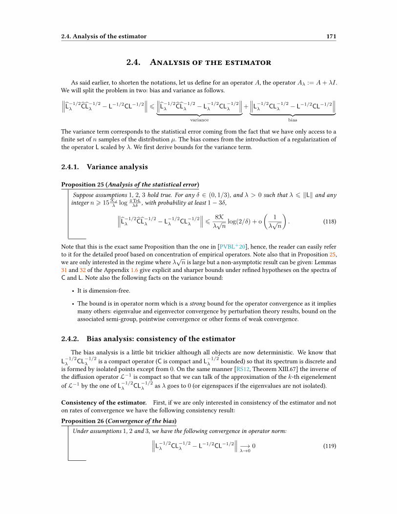
2.4. Analysis of the estimator 171
2.4. Analysis of the estimator
As said earlier, to shorten the notations, let us dene for an operator A, the operator Aλ := A+ λI .We will split the problem in two: bias and variance as follows.∥∥∥L−1/2λ CL
−1/2λ − L−1/2CL−1/2
∥∥∥ 6∥∥∥L−1/2λ CL
−1/2λ − L
−1/2λ CL
−1/2λ
∥∥∥︸ ︷︷ ︸variance
+∥∥∥L−1/2λ CL
−1/2λ − L−1/2CL−1/2
∥∥∥︸ ︷︷ ︸bias
The variance term corresponds to the statistical error coming from the fact that we have only access to anite set of n samples of the distribution µ. The bias comes from the introduction of a regularization ofthe operator L scaled by λ. We rst derive bounds for the variance term.
2.4.1. Variance analysis
Proposition 25 (Analysis of the statistical error)
Suppose assumptions 1, 2, 3 hold true. For any δ ∈ (0, 1/3), and λ > 0 such that λ 6 ‖L‖ and anyinteger n > 15Kd
λ log 4 TrLλδ , with probability at least 1− 3δ,∥∥∥L
−1/2λ CL
−1/2λ − L
−1/2λ CL
−1/2λ
∥∥∥ 68K
λ√n
log(2/δ) + o
(1
λ√n
). (118)
Note that this is the exact same Proposition than the one in [PVBL+20], hence, the reader can easily referto it for the detailed proof based on concentration of empirical operators. Note also that in Proposition 25,we are only interested in the regime where λ
√n is large but a non-asymptotic result can be given: Lemmas
31 and 32 of the Appendix 1.6 give explicit and sharper bounds under rened hypotheses on the spectra ofC and L. Note also the following facts on the variance bound:
• It is dimension-free.
• The bound is in operator norm which is a strong bound for the operator convergence as it impliesmany others: eigenvalue and eigenvector convergence by perturbation theory results, bound on theassociated semi-group, pointwise convergence or other forms of weak convergence.
2.4.2. Bias analysis: consistency of the estimator
The bias analysis is a little bit trickier although all objects are now deterministic. We know thatL−1/2λ CL
−1/2λ is a compact operator (C is compact and L
−1/2λ bounded) so that its spectrum is discrete and
is formed by isolated points except from 0. On the same manner [RS12, Theorem XIII.67] the inverse ofthe diusion operator L−1 is compact so that we can talk of the approximation of the k-th eigenelementof L−1 by the one of L
−1/2λ CL
−1/2λ as λ goes to 0 (or eigenspaces if the eigenvalues are not isolated).
Consistency of the estimator. First, if we are only interested in consistency of the estimator and noton rates of convergence we have the following consistency result:Proposition 26 (Convergence of the bias)
Under assumptions 1, 2 and 3, we have the following convergence in operator norm:∥∥∥L−1/2λ CL
−1/2λ − L−1/2CL−1/2
∥∥∥ −→λ→0
0 (119)

2.4. Analysis of the estimator 172
Note that this result was stated under the assumption that L−1/2CL−1/2 was compact in the previousSection 1. With the abstract framework developed in this section, we showed awlessly that L−1/2CL−1/2
was compact (Proposition 24), combining this new result with the proof of Proposition 13 of the previoussection, we show Proposition 26. Together with the convergence result of the variance above, this showsthat our estimate is statistically consistent when taking a sequence of regularizers such that λn → 0 andλn√n→ +∞.
2.4.3. Where this work stands: the bias analysis and the possibility of deriving
dimensionless rates of convergence.
For the whole story to be totally complete, and to highlight the dierences between our estimator andDiusion maps [CL06] (especially in high-dimension), we need to guarantee fast and explicit convergencerates. This is the case for the statistical variance term as shown in Proposition 25, but as said before,the bias term is a lot trickier and necessitates some deeper knowledge on the spectrum of the diusionoperator L. In this subsection, we will not show rigorous results as this is exactly where our currentreection lies. Yet, we will try to explain why deriving these explicit rates is a hard task and how it couldbe done in the future.
Convergence rates. Now, let us try to derive some rates of convergence for the spectrum of the biasedoperator to the true one. We will focus rst only on the top eigenvalue and eigenvector of the operator as wecan derive the same analysis with some min−max Courant-Fisher principle for the other eigenelements.
Let us denote by f∗ ∈ H1(µ) the rst eigenvector of the diusion operator to approximate and σ∗ > 0
its associated eigenvalue : Lf∗ = σ∗f∗. Similarly, let us denote fH the largest eigenvector of L−1/2λ CL
−1/2λ
and σH > 0 its associated eigenvalue. As eigenvectors are dened up to a multiplicative constant, we cannormalize them such that ‖f∗‖22 = ‖fH‖22 = 1, where the ‖ · ‖2 norm is the L2(µ) usual norm. Let usstress out that the whole story can be seen as the approximation property of the eigenfunctions of L byfunctions of the RKHS.
If f∗ belongs to the native RKHS space. As in the regression problem (either for kernel ridge regres-sion or stochastic gradient descent as described in Part III Section 2), if the function to be approximated,f∗, lies in the RKHS H, then the problem is easy and the rates of convergence are dimensionless! Moreprecisely we can show that:
|σH − σ∗| 6 λ‖f∗‖2H, (120)
Hence, if f∗ ∈ H, we have convergence of the biased operator at rate λ! The problem is that when µ haswhole support inRd then we expect the function f∗ to be regular but to not decrease at innity. For example,when µ is Gaussian, the eigenfunctions of the diusion operator L are the Hermite polynomials that do notbelong to generic RKHS such as Gaussian or Laplace. However, this case is also quite informative as whenµ has a compact support, and the potential is smooth enough (this is what is supposed in [HAL07, CL06]),then we can always take a Sobolev kernel and have f∗ ∈ H. In this case, to go further and really try to nothide the curse of dimensionality, one could try to write explicitly ‖f∗‖2H as a function of the dimension.This will depend on the tensorisation properties of the measure µ but we leave this for a future work.
If f∗ does not belong to the native RKHS space. If f∗ /∈ H, then it becomes complicated. The rstidea is to abstractly assume some approximation property of the function f∗ by the RKHS with respect tothe problem. It is exactly the purpose of the source condition in our earlier work: we formulate a generalassumption to quantify how we can really approach a function outside the RKHS (see Eq. (46) in the RKHSpart of the Introduction for a precise denition).
However, here, the function f∗ can be dened explicitly and has some interesting properties that wecould leverage: we know that it lies in H1(µ) and that being an eigenfunction of L, it has some strong

2.4. Analysis of the estimator 173
regularity. Hence, we can go deeper in the analysis and prefer a more constructive approach. Let us xε > 0, the idea is to build a function in H, namely fH such that:
(i) fH ∼ f∗ in H1(µ). Typically,∥∥∥fH − f∗∥∥∥2
H1(µ)6 ε.
(ii) ‖fH‖H is not too large. Typically,∥∥∥fH∥∥∥
H6 ε−δ , with δ > 0.
x
y f∗(x)
f(x) ∈ H
µ(x) = e−V (x)
Figure 20 – Schematic gure showing the way to approximate the rst eigenvector of the diusion operatorby a function in an RKHS. The example shows this in the case of a Gaussian measure in R for which therst eigenfunction is the monome f∗ : x→ x.
This is represented is Figure 20 and is often the way to derive bounds for general functional inequalitieswhen changing spaces of test functions, see [BGL14, p378] for such an example. In this case for theeigenvalue, we have a similar bound as previously:
|σH − σ∗| / λ‖fH‖2H, (121)
And for the eigenfunction bound, if ∠∗H is the acute angle between fH and the eigenspace associated witheigenvalue σ∗, then
sin (∠∗H) /2λ‖fH‖2H
dist(σ∗, spectrum), (122)
where dist(σ∗, spectrum) is the eigengap between the eigenspace associated to σ∗ and the rest of thespectrum.
?
? ?
2.5. Conclusion and further thoughts 174
What is proven and what remains to be: a battle for completeness. We hope tohave convinced the reader that the story behind the estimation of the whole diusion operatoris almost done. The fact that remains to be correctly stated is the approximation property of ourRKHS with respect to the eigenfunctions of the operator. To conclude this part, we really wouldlike to put emphasis that often in the learning RKHS literature, the approximation properties thatcould carry the curse of dimensionality is hidden through some technical assumption (e.g. sourcecondition). Here, as we have a strong prior on the function to be approximated, we would like totry to be as precise as possible and not rest on some technical assumption without proper intuitivemathematical content.
2.5. Conclusion and further thoughts
Comparison to Diusion maps. In this work, we tried to prove that we could estimate the eigenele-ments of the diusion operator. This construction relies on positive kernel methods on the contrary toolder methods relying on local averaging techniques. This could lead to ecient and robust estimation inhigher dimension in comparison to Diusion maps [CL06]. However, to really compare to this celebratedwork, further paths should be explored, and one of the most important is that Diusion maps can haveaccess to the geometric structure of the data with an appropriate reweighting. Is this possible to do thesame with our technique?
The kernel choice. Another discussion that we only sketched is the crucial choice of the kernel in sucha situation. As recalled throughout the Introduction, the art of kernel engineering is a central question toapply psd kernel methods. For this problem, the kernel should be respecting two guidelines: (i) it shouldhave a Mercer decomposition with explicit features (random or appropriately chosen features). Indeed, weneed to build the covariance matrix with respect to the derivative kernel L that can be very costly if wedo not have explicit features. More precisely if we approximate our kernel with M features we go fromsize O(nM) to O(n2d) matrix: this saves a huge cost. (ii) As explained in the last subsection, the RKHSshould be chosen to approximate well the eigenfunctions of the diusion operator in H1(µ). Remark thatthe weakness of the RKHS comes this time from the decreasing at innity and not from the regularity.This should enable dimensionless approach in most of the cases.
Tensorisation property. To go as deep as it can be, an important property of eigenelements of thediusion operator is its tensorisation nature: if µ is a tensor product measure over Rd then the eigen-functions will have also a tensorized form and lie in low-dimensional spaces. This should be taken intoaccount when designing the kernel: it should leverage this possible tensorisation property to exploit thelow-dimensional structure of the object.
Other works. A recent literature in applied probability aims at estimating the spectral gaps of MarkovChain given the rst n iterates of it [HKS15]. Our procedure seems to do exactly the same, and understand-ing the dierence between our algorithm and theirs is something we have to explore. This will require toadapt a bit our algorithm and change our i.i.d. assumption on the samples to a Markovian one.
?
? ?

This is a fucking blank sentence.
175

Part IV
Conclusion and future work
1. Summary of the thesis
In the course of this manuscript, we have investigated two topics. First, we focused on the convergenceproperties of the stochastic gradient descent algorithm in Hilbert spaces. Second, we have studieddimensionality-reduction techniques through the estimation of the Laplacian operator associated to thedata. In this context, we also have come up with a new algorithm to estimate this latter operator and explainthat leveraging this knowledge could lead to accelerate Monte Carlo Markov Chains in high-dimension.Note that for these two directions, even if my background and personal preferences has driven me moreto modelling and theoretical questions, I have also been concerned with the numerical eciency of thealgorithms involved and their implementation.
To summarize more precisely the contributions of this thesis, let us dive rst into the optimizationframework at stake when it comes to solve high-dimensional supervised learning problems. In supervisedlearning, stochastic gradient methods are ubiquitous, both from the practical side, as a simple algorithmthat can learn from a single or a few passes over the data, and from the theoretical side, as it leads tooptimal rates for estimation problems in a variety of situations.
In this context, we rst showed that, under a margin assumption [AT07], for classication problems,the classication error of the averaged iterates of stochastic gradient descent converge exponentially fastto the best achievable error although the regression error had only a O(1/n) convergence rate, henceestablishing theoretically a largely observed behavior in practice.
One of the eorts in theoretical machine learning is to understand or improve the empirical rules ofpractitioners. However, until our second contribution, theory predicted that practitioners should stop thestochastic gradient descent iterations after having only seen once the whole data-set (∼ n iterations). Thesecond contribution of this thesis establishes some map on the hardness of a learning problem and showedthat for hard problems, it was necessary to stop stochastic gradient descent only after several passes overthe whole data-set reconciling on this aspect theory and practice. Stating optimality in the context of non-parametric regression requires both a source condition (which quanties the smoothness of the optimalprediction function) and a capacity condition (related to the eigenvalue decay of the covariance operators).
176

2. PERSPECTIVES 177
We show that multiple-pass averaging, combined with larger step sizes than traditional approaches, allowsto get this optimal behavior.
In a second direction, we worked on a new kernel-based algorithm for unsupervised learning. Thisproject was initiated by discussions with researchers in molecular dynamics (Tony Lelièvre and GabrielStoltz) to nd reaction coordinates in molecular systems which are central objects to simulate ecientlyand understand such systems. This project gave birth to a new practical algorithm that could have a largearea of applications. Indeed, based on a variational formulation of the underlying diusion operator thatgenerated the samples, we designed a dimensionality-reduction algorithm. One of the main result of thisproject is that we estimated with a kernel-based method (thus avoiding the curse of dimensionality andhard parameter tuning as in previous approaches [CL06]) the innitesimal operator of the overdampedLangevin diusion (or general Laplacian). The eigenelements of such an operator are the cornerstone ofclustering or dimensionality reduction techniques.
?
? ?
2. Perspectives
We have already largely developed in the introduction possible future works, by putting emphasis oninteresting unexplored directions. Among them, we have already spoken of my personal interest for thecontinuous dynamics behind SGD iterations in subsection 2.2.2, the art of engineering kernels that canmimic the expressivity of neural networks in subsection 3.3.2, or the link between statistical physics andMachine Learning in subsection 4.1.2. In this perspective part, even if it is a crucial point and a possiblefuture direction in my academic career, I will not dwell into the kernel topic. I refer to 3.3.2 for detaildiscussions on it.
To expose clearly the future works that I will be probably conducting during the following months, letus divide them in the two directions taken during this thesis.
Stochastic gradient descent. Let us explain the questions triggered by our contribution on this aspect.
1. Optimality for classication problems. In the second work on stochastic gradient descent, the funda-mental question was optimality of SGD, whereas we only showed “fast rates” for the classicationerror in the rst work. A natural idea would be to merge these two works wondering if we canreach optimality with SGD for classication problems under low noise conditions.
2. Continuous-time SGD dynamics. The Langevin dynamics seems very related to stochastic gradientdescent with additive noise as we have seen in Section 2 of this introduction. In this same direction,understanding continuous versions of the algorithms often leads to a deeper comprehension of thebehavior of the systems. This could lead to the study of the continuous counterpart of the stochasticgradient descent algorithm [LT19]. Continuing further the discussion introduced in subsection 2.2.2is one of the rst questions I will be studying in the short-time future.
3. Noiseless setting. Lately, the community has been curious about the “noiseless setting” [BBG20,VBS19] where the only source of noise in the recursion is multiplicative. In this setting, there issome lack of knowledge, in particular concerning minimax rates or how the implicit bias of SGDcan lead to good generalization error. Digging in this direction seems to be promising to understandthe impact of the noise is ML models and the good generalization properties of SGD.

2. PERSPECTIVES 178
Estimation of Laplacian and dimensionality reduction. We distinguish here three possible exten-sions of our work:
1. Finishing current work ! The rst thing would obviously be to nish the work presented in Section 2of Part III. Showing its applicability in molecular dynamics and relevance in the statistics communityis the rst thing I will consider doing.
2. Approximation of the Laplace-Beltrami operator. We have developed a kernel method to build fromsamples the diusion operator associated with the measure that produced them. For data distributedaccording to a particular geometry, it seems possible to extend our procedure to construct anapproximation of the Laplace-Beltrami operator associated with the sub-manifold to which thesedata belong. The Laplace-Beltrami operator estimation is the cornerstone of geometric data analysisapproaches and clustering methods widely used in practice [VL07]. The construction of theseoperators from psd kernels would possibly allow to avoid the curse of dimensionality, on thecontrary of currently used local averaging methods [HAL07, CL06]. Showing the consistency ofsuch estimates of operators or of their spectral elements (eigenvectors and values) requires detailedknowledge of spectral approximation methods.
3. Acceleration of sampling procedures. As discussed in the introduction, one of the main problemsof sampling large dimensional non-strongly logarithmic concave measures is that the dynamicsused to sample the said measure can get stuck for a long time in localized modes of the distribution.This phenomenon is called metastability (see Section 4.3 for details). To speed up such samplingprocedures, one of the common techniques in molecular dynamics is to use importance samplingstrategies by biasing the target measure by a low-dimensional function representing the slowdirections of diusion (free energy associated with a reaction coordinate). The estimation of thesereaction coordinates therefore allows the use of acceleration methods for the sampling of multimodalmeasurements. If in this thesis, we implemented numerically the estimation of coordinates of linearand low-dimensional reactions in an idealized framework (mixture of three Gaussians in dimension2), the objective is to develop this procedure in more realistic cases corresponding to real molecularsystems (with applications in pharmacology) or to sample the a posteriori laws of the parameters ofGaussian mixtures within the framework of Bayesian inference [CLS12]. Two important obstaclesmust be removed for the practical application of the procedure: being able to estimate reactioncoordinates (i) in high dimension and (ii) that could potentially be non-linear.
Learning/statistical physics interaction. In the medium term, I would like to work on problems atthe interface between statistical physics, molecular dynamics and learning. Indeed, in addition to theapproaches based on the estimation of a diusion operator mentioned above, many links exist betweenstatistical learning and statistical physics. Moreover, even if the objectives of the two disciplines aredierent, the dynamics under study in statistical physics can be seen as the continuous counterpart ofthe stochastic gradient descent. The large dimension and the metastability of such dynamics, especiallyin the case of Bayesian inference in large dimension are important aspects common to both disciplinesand the acceleration techniques developed in molecular dynamics could be extensively used to solvelearning problems. More importantly, one active eld of study in statistical physics and Machine Learningis to try to accelerate the stochastic dynamics at hand. These techniques rely on changing it withoutaecting the invariant measure while accelerating the convergence to equilibrium. We could (i) studyKinetic versions of Langevin dynamics [MCC+19], (ii) add some drift term or (iii) some non-reversibilitythrough birth-and-death processes [LLN19]. How do these techniques transfer for stochastic optimizationpurposes ?
?? ?

This is a fucking blank sentence.
179

REFERENCES 180
References
[ADT20] Alnur Ali, Edgar Dobriban, and Ryan J Tibshirani. The implicit regularization of stochasticgradient ow for least squares. arXiv preprint arXiv:2003.07802, 2020.
[AF03] Robert A. Adams and John J.F. Fournier. Sobolev spaces, volume 140. Academic Press, 2003.
[AMP00] R. Aguech, E. Moulines, and P. Priouret. On a perturbation approach for the analysis ofstochastic tracking algorithms. SIAM J. Control and Optimization, 39(3):872–899, 2000.
[Aro50] Nachman Aronszajn. Theory of reproducing kernels. Transactions of the American mathe-matical society, 68(3):337–404, 1950.
[AT07] Jean-Yves Audibert and Alexandre B. Tsybakov. Fast learning rates for plug-in classiers.The Annals of statistics, 35(2):608–633, 2007.
[AZO14] Zeyuan Allen-Zhu and Lorenzo Orecchia. Linear coupling: An ultimate unication of gradientand mirror descent. arXiv preprint arXiv:1407.1537, 2014.
[Bac14] Francis Bach. Adaptivity of averaged stochastic gradient descent to local strong convexityfor logistic regression. Journal of Machine Learning Research, 15(19):595–627, 2014.
[Bac17] Francis Bach. On the equivalence between kernel quadrature rules and random featureexpansions. Journal of Machine Learning Research, 18(21):1–38, 2017.
[BB08] Léon Bottou and Olivier Bousquet. The tradeos of large scale learning. In Advances inneural information processing systems, pages 161–168, 2008.
[BBG20] Raphaël Berthier, Francis Bach, and Pierre Gaillard. Tight nonparametric convergence ratesfor stochastic gradient descent under the noiseless linear model, 2020.
[BBM05] Peter L. Bartlett, Olivier Bousquet, and Shahar Mendelson. Local rademacher complexities.Ann. Statist., 33(4):1497–1537, 08 2005.
[BBV04] Stephen Boyd, Stephen P Boyd, and Lieven Vandenberghe. Convex optimization. Cambridgeuniversity press, 2004.
[BCN18] Léon Bottou, Frank E Curtis, and Jorge Nocedal. Optimization methods for large-scalemachine learning. SIAM Review, 60(2):223–311, 2018.
[BGL14] Dominique Bakry, Ivan Gentil, and Michel Ledoux. Analysis andGeometry ofMarkov DiusionOperators. Springer, 2014.
[Bis95] Chris M Bishop. Training with noise is equivalent to tikhonov regularization. Neuralcomputation, 7(1):108–116, 1995.
[BJM06] Peter L. Bartlett, Michael I. Jordan, and Jon D. McAulie. Convexity, classication, and riskbounds. Journal of the American Statistical Association, 101(473):138–156, 2006.
[BK16] Gilles Blanchard and Nicole Krämer. Convergence rates of kernel conjugate gradient forrandom design regression. Analysis and Applications, 14(06):763–794, 2016.
[BLC05] L. Bottou and Y. Le Cun. On-line learning for very large data sets. Applied Stochastic Modelsin Business and Industry, 21(2):137–151, 2005.
[BLJ04] Francis R Bach, Gert RG Lanckriet, and Michael I Jordan. Multiple kernel learning, conicduality, and the smo algorithm. In Proceedings of the twenty-rst international conference onMachine learning, page 6, 2004.

REFERENCES 181
[BLS15] Sébastien Bubeck, Yin Tat Lee, and Mohit Singh. A geometric alternative to nesterov’saccelerated gradient descent. arXiv preprint arXiv:1506.08187, 2015.
[BM11] F. Bach and E. Moulines. Non-asymptotic analysis of stochastic approximation algorithmsfor machine learning. In Advances in Neural Information Processing Systems (NIPS), 2011.
[BM13] Francis Bach and Eric Moulines. Non-strongly-convex smooth stochastic approximationwith convergence rate O(1/n). In Advances in Neural Information Processing Systems (NIPS),pages 773–781, 2013.
[BM17] Gilles Blanchard and Nicole Mücke. Optimal rates for regularization of statistical inverselearning problems. Foundations of Computational Mathematics, pages 1–43, 2017.
[BMAS14] Nicolas Boumal, Bamdev Mishra, P.-A. Absil, and Rodolphe Sepulchre. Manopt, a Matlabtoolbox for optimization on manifolds. Journal of Machine Learning Research, 15:1455–1459,2014.
[Bob99] Sergey G. Bobkov. Isoperimetric and analytic inequalities for log-concave probability mea-sures. Ann. Probab., 27:1903–1921, 1999.
[Boy04] Stephen Boyd. Subgradient methods. 2004.
[BRH13] Nawaf Bou-Rabee and Martin Hairer. Nonasymptotic mixing of the mala algorithm. IMAJournal of Numerical Analysis, 33(1):80–110, 2013.
[CB20] Lenaic Chizat and Francis Bach. Implicit bias of gradient descent for wide two-layer neuralnetworks trained with the logistic loss. arXiv preprint arXiv:2002.04486, 2020.
[CBLK06] Ronald Coifman, Nadler Boaz, Stéphane Lafon, and Ioannis Kevrekidis. Diusion maps,spectral clustering and reaction coordinates of dynamical systems. Applied and ComputationalHarmonic Analysis, 21(12):113–127, 2006.
[CBR18] Carlo Ciliberto, Francis Bach, and Alessandro Rudi. Localized structured prediction. arXivpreprint arXiv:1806.02402, 2018.
[CCS+19] Pratik Chaudhari, Anna Choromanska, Stefano Soatto, Yann LeCun, Carlo Baldassi, Chris-tian Borgs, Jennifer Chayes, Levent Sagun, and Riccardo Zecchina. Entropy-sgd: Biasinggradient descent into wide valleys. Journal of Statistical Mechanics: Theory and Experiment,2019(12):124018, 2019.
[CDV07] Andrea Caponnetto and Ernesto De Vito. Optimal rates for the regularized least-squaresalgorithm. Foundations of Computational Mathematics, 7(3):331–368, 2007.
[CFG+20] Benjamin Charlier, Jean Feydy, Joan Alexis Glaunès, François-David Collin, and GhislainDurif. Kernel operations on the gpu, with autodi, without memory overows, 2020.
[Che81] Herman Cherno. A note on an inequality involving the normal distribution. Ann. Probab.,9(3):533–535, 1981.
[CL06] Ronald R. Coifman and Stéphane Lafon. Diusion maps. Applied and Computational HarmonicAnalysis, 21(1), 2006.
[CLS12] Nicolas Chopin, Tony Lelièvre, and Gabriel Stoltz. Free energy methods for Bayesian inference:ecient exploration of univariate Gaussian mixture posteriors. Statistics and Computing,22(4):897–916, 2012.
[CM10] Djalil Chafaï and Florent Malrieu. On ne properties of mixtures with respect to concentrationof measure and Sobolev type inequalities. Annales de l’Institut Henri Poincaré, Probabilités etStatistiques, 46:72–96, 2010.

REFERENCES 182
[Cra76] Charles R Crawford. A stable generalized eigenvalue problem. SIAM Journal on NumericalAnalysis, 13(6):854–860, 1976.
[CRR16] Carlo Ciliberto, Lorenzo Rosasco, and Alessandro Rudi. A consistent regularization approachfor structured prediction. In Advances in Neural Information Processing Systems, 2016.
[CRR18] Luigi Carratino, Alessandro Rudi, and Lorenzo Rosasco. Learning with sgd and randomfeatures. arXiv preprint arXiv:1807.06343, 2018.
[CRRP17] Carlo Ciliberto, Alessandro Rudi, Lorenzo Rosasco, and Massimiliano Pontil. Consistent mul-titask learning with nonlinear output relations. In Advances in Neural Information ProcessingSystems, pages 1986–1996, 2017.
[CT19] Richard Combes and Mikael Touati. Computationally ecient estimation of the spectralgap of a markov chain. Proceedings of the ACM on Measurement and Analysis of ComputingSystems, 3(1):7, 2019.
[Dal17] Arnak Dalalyan. Further and stronger analogy between sampling and optimization: Langevinmonte carlo and gradient descent. In Proceedings of the 2017 Conference on Learning Theory,volume 65 of Proceedings of Machine Learning Research, pages 678–689. PMLR, 07–10 Jul 2017.
[Dau92] Ingrid Daubechies. Ten lectures on wavelets. SIAM, 1992.
[DB15] A. Défossez and F. Bach. Constant step size least-mean-square: Bias-variance trade-os andoptimal sampling distributions. In Proc. AISTATS, 2015.
[DB16] Aymeric Dieuleveut and Francis Bach. Nonparametric stochastic approximation with largestep-sizes. The Annals of Statistics, 44(4):1363–1399, 2016.
[DBLJ14] Aaron Defazio, Francis Bach, and Simon Lacoste-Julien. SAGA: A fast incremental gradientmethod with support for non-strongly convex composite objectives. In Advances in NeuralInformation Processing Systems, 2014.
[DDB17] Aymeric Dieuleveut, Alain Durmus, and Francis Bach. Bridging the gap between constantstep size stochastic gradient descent and markov chains. arXiv preprint arXiv:1707.06386,2017.
[DFB17] Aymeric Dieuleveut, Nicolas Flammarion, and Francis Bach. Harder, better, faster, strongerconvergence rates for least-squares regression. Journal of Machine Learning Research, pages1–51, 2017.
[DGL13] Luc Devroye, László Györ, and Gábor Lugosi. A Probabilistic Theory of Pattern Recognition,volume 31. Springer Science & Business Media, 2013.
[Die17] Aymeric Dieuleuveut. Stochastic approximation in Hilbert spaces. PhD thesis, ENS - INRIA,2017.
[DM17] Alain Durmus and Eric Moulines. Nonasymptotic convergence analysis for the unadjustedLangevin algorithm. Annals of Applied Probability, 27(3):1551–1587, 2017.
[DM19] Alain Durmus and Eric Moulines. High-dimensional Bayesian inference via the unadjustedLangevin algorithm. Bernoulli, 25(4A):2854–2882, 2019.
[DRVZ17] Alain Durmus, Gareth O. Roberts, Gilles Vilmart, and Konstantinos C. Zygalakis. FastLangevin based algorithm for mcmc in high dimensions. Ann. Appl. Probab., 27(4):2195–2237,08 2017.

REFERENCES 183
[DVRT14] Ernesto De Vito, Lorenzo Rosasco, and Alessandro Toigo. Learning sets with separatingkernels. Applied and Computational Harmonic Analysis, 37(2):185–217, 2014.
[EAS98] Alan Edelman, Tomás A. Arias, and Steven T. Smith. The geometry of algorithms withorthogonality constraints. SIAM journal on Matrix Analysis and Applications, 20(2):303–353,1998.
[EK+10] Noureddine El Karoui et al. The spectrum of kernel random matrices. The Annals of Statistics,38(1):1–50, 2010.
[FBG07] Kenji Fukumizu, Francis Bach, and Arthur Gretton. Statistical consistency of kernel canonicalcorrelation analysis. Journal of Machine Learning Research, 8:361–383, 2007.
[FBJ04] Kenji Fukumizu, Francis Bach, and Michael I. Jordan. Dimensionality reduction for supervisedlearning with reproducing kernel Hilbert spaces. Journal of Machine Learning Research,5(Jan):73–99, 2004.
[FS01] Daan Frenkel and Berend Smit. Understanding Molecular Simulation: From Algorithms toApplications, volume 1. Elsevier, 2001.
[FS17] Simon Fischer and Ingo Steinwart. Sobolev norm learning rates for regularized least-squaresalgorithm. Technical Report 1702.07254, arXiv, 2017.
[FW98] Mark Iosifovich Freidlin and Alexander D Wentzell. Random perturbations. In Randomperturbations of dynamical systems, pages 15–43. Springer, 1998.
[G+] Andreas Griewank et al. On automatic dierentiation.
[Gan10] Klaus Gansberger. An idea on proving weighted Sobolev embeddings. arXiv:1007.3525., 2010.
[GBR+12] Arthur Gretton, Karsten M Borgwardt, Malte J Rasch, Bernhard Schölkopf, and AlexanderSmola. A kernel two-sample test. The Journal of Machine Learning Research, 13(1):723–773,2012.
[Gke19] Paraskevi Gkeka. Machine learning force eld and coarse-grained variables in moleculardynamics: application to materials and biological systems. Preprint, 2019.
[GL06] Dani Gamerman and Hedibert Lopes. Markov Chain Monte Carlo: Stochastic Simulation forBayesian Inference. Chapman and Hall/CRC, 2006.
[GOP15] Mert Gürbüzbalaban, Asu Ozdaglar, and Pablo Parrilo. Why random reshuing beatsstochastic gradient descent. Technical Report 1510.08560, arXiv, 2015.
[Goz10] Nathael Gozlan. Poincaré inequalities and dimension free concentration of measure. Ann.Inst. H. Poincaré Probab. Statist., 46(3):708–739, 2010.
[GRO+08] L Lo Gerfo, L Rosasco, F Odone, E De Vito, and A Verri. Spectral algorithms for supervisedlearning. Neural Computation, 20(7):1873–1897, 2008.
[GRS95] Walter Gilks, Sylvia Richardson, and David Spiegelhalter. Markov Chain Monte Carlo inPractice. Chapman and Hall/CRC, 1995.
[GT01] David Gilbarg and Neil S. Trudinger. Elliptic Partial Dierential Equations of Second Order.Springer Berlin Heidelberg, 2001.
[Gu13] Chong Gu. Smoothing spline ANOVAmodels, volume 297. Springer Science & Business Media,2013.

REFERENCES 184
[HAL07] Matthias Hein, Jean-Yves Audibert, and Ulrike von Luxburg. Graph laplacians and theirconvergence on random neighborhood graphs. Journal of Machine Learning Research, pages1325–1368, 2007.
[HKS15] Daniel Hsu, Aryeh Kontorovich, and Csaba Szepesvári. Mixing time estimation in reversiblemarkov chains from a single sample path. In Advances in neural information processingsystems, pages 1459–1467, 2015.
[HN92] Robert Hecht-Nielsen. Theory of the backpropagation neural network. In Neural networksfor perception, pages 65–93. Elsevier, 1992.
[HN05] Bernard Heler and Francis Nier. Hypoelliptic estimates and spectral theory for Fokker-Planckoperators and Witten Laplacians. Lecture Notes in Mathematics, 1862, 2005.
[Hot33] Harold Hotelling. Analysis of a complex of statistical variables into principal components.Journal of educational psychology, 24(6):417, 1933.
[HRS16] Moritz Hardt, Ben Recht, and Yoram Singer. Train faster, generalize better: Stability ofstochastic gradient descent. In International Conference on Machine Learning, 2016.
[HTF09] Trevor Hastie, Robert Tibshirani, and Jerome Friedman. The elements of statistical learning:data mining, inference, and prediction. Springer Science & Business Media, 2009.
[IL67] Alekse Grigorevich Ivakhnenko and Valentin Grigorevich Lapa. Cybernetics and forecastingtechniques. 1967.
[JGH18] Arthur Jacot, Franck Gabriel, and Clément Hongler. Neural tangent kernel: Convergenceand generalization in neural networks. In Advances in neural information processing systems,pages 8571–8580, 2018.
[JK17] Prateek Jain and Purushottam Kar. Non-convex optimization for machine learning. Founda-tions and Trends in Machine Learning, 10(3-4):142–336, 2017.
[JKK+16] Prateek Jain, Sham M. Kakade, Rahul Kidambi, Praneeth Netrapalli, and Aaron Sidford.Parallelizing stochastic approximation through mini-batching and tail-averaging. TechnicalReport 1610.03774, arXiv, 2016.
[JNN19] Prateek Jain, Dheeraj Nagaraj, and Praneeth Netrapalli. Making the last iterate of sgdinformation theoretically optimal. In Conference on Learning Theory, pages 1752–1755, 2019.
[JZ13] Rie Johnson and Tong Zhang. Accelerating stochastic gradient descent using predictivevariance reduction. In Advances in Neural Information Processing Systems, 2013.
[KB05] Vladimir Koltchinskii and Olexandra Beznosova. Exponential convergence rates in classica-tion. In International Conference on Computational Learning Theory. Springer, 2005.
[KP13] Peter E Kloeden and Eckhard Platen. Numerical solution of stochastic dierential equations,volume 23. Springer Science & Business Media, 2013.
[KT09] Sham M. Kakade and Ambuj Tewari. On the generalization ability of online strongly convexprogramming algorithms. In Advances in Neural Information Processing Systems, 2009.
[Lan12] Guanghui Lan. An optimal method for stochastic composite optimization. MathematicalProgramming, 133(1-2):365–397, 2012.
[LBH15] Yann LeCun, Yoshua Bengio, and Georey Hinton. Deep learning. nature, 521(7553):436–444,2015.

REFERENCES 185
[Led14] Michel Ledoux. Concentration of measure and logarithmic Sobolev inequalities. Séminairede Probas XXXIII, pages 120–216, 2014.
[Lel09] Tony Lelièvre. A general two-scale criteria for logarithmic Sobolev inequalities. Journal ofFunctional Analysis, 256(7):2211 – 2221, 2009.
[Lel13] Tony Lelièvre. Two mathematical tools to analyze metastable stochastic processes. InNumerical Mathematics and Advanced Applications 2011, pages 791–810, Berlin, Heidelberg,2013. Springer.
[Lel15] Tony Lelièvre. Accelerated dynamics: Mathematical foundations and algorithmic improve-ments. The European Physical Journal Special Topics, 224(12):2429–2444, 2015.
[LJSB12] Simon Lacoste-Julien, Mark Schmidt, and Francis Bach. A simpler approach to obtainingan o (1/t) convergence rate for the projected stochastic subgradient method. arXiv preprintarXiv:1212.2002, 2012.
[LLN19] Yulong Lu, Jianfeng Lu, and James Nolen. Accelerating Langevin sampling with birth-death.arXiv preprint arXiv:1905.09863, 2019.
[LM+16] Guillaume Lecué, Shahar Mendelson, et al. Performance of empirical risk minimization inlinear aggregation. Bernoulli, 22(3):1520–1534, 2016.
[LP16] David Levin and Yuval Peres. Estimating the spectral gap of a reversible markov chain froma short trajectory. arXiv preprint 1612.05330, 2016.
[LR17] Junhong Lin and Lorenzo Rosasco. Optimal rates for multi-pass stochastic gradient methods.Journal of Machine Learning Research, 18(97):1–47, 2017.
[LRRC18] Junhong Lin, Alessandro Rudi, Lorenzo Rosasco, and Volkan Cevher. Optimal rates for spectralalgorithms with least-squares regression over hilbert spaces. Applied and ComputationalHarmonic Analysis, 2018.
[LRS08] Tony Lelièvre, Mathias Rousset, and Gabriel Stoltz. Long-time convergence of an adaptivebiasing force method. Nonlinearity, 21(6):1155, 2008.
[LS16] Tony Lelièvre and Gabriel Stoltz. Partial dierential equations and stochastic methods inmolecular dynamics. Acta Numerica, 25:681–880, 2016.
[LT19] Qianxiao Li and Cheng Tai. Stochastic modied equations and dynamics of stochastic gradientalgorithms I: Mathematical foundations. J. Mach. Learn. Res., 20:40–1, 2019.
[MCC+19] Yi-An Ma, Niladri Chatterji, Xiang Cheng, Nicolas Flammarion, Peter Bartlett, andMichael I Jordan. Is there an analog of Nesterov acceleration for MCMC? arXiv preprintarXiv:1902.00996, 2019.
[MCJ+18] Yi-An Ma, Yuansi Chen, Chi Jin, Nicolas Flammarion, and Michael I. Jordan. Sampling can befaster than optimization. arXiv preprint arXiv:1612.05330, 2018.
[MCRR20] Giacomo Meanti, Luigi Carratino, Lorenzo Rosasco, and Alessandro Rudi. Kernel methodsthrough the roof: handling billions of points eciently. 2020.
[MFSS17] K Muandet, K Fukumizu, B Sriperumbudur, and B Schölkopf. Kernel mean embedding ofdistributions: A review and beyond. Foundations and Trends in Machine Learning, 10(1-2):1–144, 2017.
[MHB17] Stephan Mandt, Matthew D. Homan, and David M. Blei. Stochastic gradient descent asapproximate Bayesian inference. J. Mach. Learn. Res., 18(1):4873–4907, January 2017.

REFERENCES 186
[MKHS14] Julien Mairal, Piotr Koniusz, Zaid Harchaoui, and Cordelia Schmid. Convolutional kernelnetworks. In Advances in neural information processing systems, pages 2627–2635, 2014.
[MM19] Song Mei and Andrea Montanari. The generalization error of random features regression:Precise asymptotics and double descent curve. arXiv preprint arXiv:1908.05355, 2019.
[MS14] Georg Menz and André Schlichting. Poincaré and logarithmic Sobolev inequalities bydecomposition of the energy landscape. Ann. Probab., 42(5):1809–1884, 09 2014.
[MSS+99] Sebastian Mika, Bernhard Schölkopf, Alex J Smola, Klaus-Robert Müller, Matthias Scholz,and Gunnar Rätsch. Kernel pca and de-noising in feature spaces. In Advances in neuralinformation processing systems, pages 536–542, 1999.
[MT99] Enno Mammen and Alexandre Tsybakov. Smooth discrimination analysis. The Annals ofStatistics, 27(6):1808–1829, 1999.
[MT12] Sean P. Meyn and Richard L. Tweedie. Markov Chains and Stochastic Stability. SpringerScience & Business Media, 2012.
[MT20] Per-Gunnar Martinsson and Joel Tropp. Randomized numerical linear algebra: Foundations& algorithms. arXiv preprint arXiv:2002.01387, 2020.
[Mur12] Kevin P. Murphy. Machine Learning: a Probabilistic Perspective. MIT Press, 2012.
[MXZ06] Charles A Micchelli, Yuesheng Xu, and Haizhang Zhang. Universal kernels. Journal ofMachine Learning Research, 7(Dec):2651–2667, 2006.
[Nad64] Elizbar A Nadaraya. On estimating regression. Theory of Probability & Its Applications,9(1):141–142, 1964.
[Nes83] Yurii Nesterov. A method for unconstrained convex minimization problem with the rate ofconvergence o (1/kˆ 2). In Doklady an ussr, volume 269, pages 543–547, 1983.
[Nes12] Yu Nesterov. Eciency of coordinate descent methods on huge-scale optimization problems.SIAM Journal on Optimization, 22(2):341–362, 2012.
[NJLS09] A. Nemirovski, A. Juditsky, G. Lan, and A. Shapiro. Robust stochastic approximation approachto stochastic programming. SIAM Journal on Optimization, 19(4):1574–1609, 2009.
[NV08] Y. Nesterov and J. P. Vial. Condence level solutions for stochastic programming. Automatica,44(6):1559–1568, 2008.
[NY83] A. S. Nemirovski and D. B. Yudin. Problem complexity and method eciency in optimization.John Wiley, 1983.
[OBLJ17] Anton Osokin, Francis Bach, and Simon Lacoste-Julien. On structured prediction theory withcalibrated convex surrogate losses. In Advances in Neural Information Processing Systems,2017.
[Opf06] Roland Opfer. Multiscale kernels. Advances in computational mathematics, 25(4):357–380,2006.
[OR07] Felix Otto and Maria G. Rezniko. A new criterion for the logarithmic Sobolev inequalityand two applications. Journal of Functional Analysis, 243(1):121–157, 2007.
[Pea01] Karl Pearson. Liii. on lines and planes of closest t to systems of points in space. The London,Edinburgh, and Dublin Philosophical Magazine and Journal of Science, 2(11):559–572, 1901.

REFERENCES 187
[P86] Georg Ch Pug. Stochastic minimization with constant step-size: asymptotic laws. SIAMJournal on Control and Optimization, 24(4):655–666, 1986.
[PGC+17] Adam Paszke, Sam Gross, Soumith Chintala, Gregory Chanan, Edward Yang, Zachary DeVito,Zeming Lin, Alban Desmaison, Luca Antiga, and Adam Lerer. Automatic dierentiation inpytorch. 2017.
[Pin94] Iosif Pinelis. Optimum bounds for the distributions of martingales in banach spaces. TheAnnals of Probability, pages 1679–1706, 1994.
[PJ92] B. T. Polyak and A. B. Juditsky. Acceleration of stochastic approximation by averaging. SIAMJournal on Control and Optimization, 30(4):838–855, 1992.
[Pol64] Boris T Polyak. Some methods of speeding up the convergence of iteration methods. USSRComputational Mathematics and Mathematical Physics, 4(5):1–17, 1964.
[PVBL+20] Loucas Pillaud-Vivien, Francis Bach, Tony Lelièvre, Alessandro Rudi, and Gabriel Stoltz.Statistical estimation of the Poincaré constant and application to sampling multimodaldistributions. In International Conference on Articial Intelligence and Statistics, pages 2753–2763, 2020.
[PVRB18] Loucas Pillaud-Vivien, Alessandro Rudi, and Francis Bach. Exponential convergence of testingerror for stochastic gradient methods. In Proceedings of the 31st Conference On LearningTheory, volume 75, pages 250–296, 2018.
[QHK+19] Qian Qin, James P Hobert, Kshitij Khare, et al. Estimating the spectral gap of a trace-classmarkov operator. Electronic Journal of Statistics, 13(1):1790–1822, 2019.
[RBV10] Lorenzo Rosasco, Mikhail Belkin, and Ernesto De Vito. On learning with integral operators.Journal of Machine Learning Research, 11(Feb):905–934, 2010.
[RCDVR14] Alessandro Rudi, Guillermo D Canas, Ernesto De Vito, and Lorenzo Rosasco. Learning setsand subspaces. Regularization, Optimization, Kernels, and Support Vector Machines, pages337–357, 2014.
[RCR13] Alessandro Rudi, Guillermo D Canas, and Lorenzo Rosasco. On the sample complexity ofsubspace learning. In Advances in Neural Information Processing Systems, pages 2067–2075,2013.
[RCR15] Alessandro Rudi, Raaello Camoriano, and Lorenzo Rosasco. Less is more: Nyström computa-tional regularization. In Advances in Neural Information Processing Systems, pages 1657–1665,2015.
[RCR17] Alessandro Rudi, Luigi Carratino, and Lorenzo Rosasco. Falkon: An optimal large scale kernelmethod. In Advances in Neural Information Processing Systems, pages 3888–3898, 2017.
[RLM95] Kannan Ravindran, Lovasz Laszlo, and Simonovits Miklos. Isoperimetric problems for convexbodies and a localization lemma. Discrete Comput. Geom., 13(3):541–559, 1995.
[RM51] H. Robbins and S. Monro. A stochastic approximation method. Ann. Math. Statistics, 22:400–407, 1951.
[Rob07] Christian Robert. The Bayesian Choice: from Decision-theoretic Foundations to ComputationalImplementation. Springer Science & Business Media, 2007.
[RR08] Ali Rahimi and Benjamin Recht. Random features for large-scale kernel machines. InAdvances in neural information processing systems, pages 1177–1184, 2008.

REFERENCES 188
[RR17] Alessandro Rudi and Lorenzo Rosasco. Generalization properties of learning with randomfeatures. In Advances in Neural Information Processing Systems, pages 3218–3228, 2017.
[RRT17] Maxim Raginsky, Alexander Rakhlin, and Matus Telgarsky. Non-convex learning via stochas-tic gradient Langevin dynamics: a nonasymptotic analysis. In Satyen Kale and Ohad Shamir,editors, Proceedings of the 2017 Conference on Learning Theory, volume 65 of Proceedingsof Machine Learning Research, pages 1674–1703, Amsterdam, Netherlands, 07–10 Jul 2017.PMLR.
[RS12] Michael Reed and Barry Simon. Methods of ModernMathematical Physics: Functional Analysis,volume IV. Elsevier, 2012.
[RSB12] Nicolas L. Roux, Mark Schmidt, and Francis Bach. A stochastic gradient method with anexponential convergence rate for nite training sets. In Advances in Neural InformationProcessing Systems (NIPS), 2012.
[RSS12] Alexander Rakhlin, Ohad Shamir, and Karthik Sridharan. Making gradient descent optimalfor strongly convex stochastic optimization. In Proceedings of the 29th International Coferenceon International Conference on Machine Learning, pages 1571–1578, 2012.
[RT14] Peter Richtárik and Martin Takáč. Iteration complexity of randomized block-coordinatedescent methods for minimizing a composite function. Mathematical Programming, 144(1-2):1–38, 2014.
[RV15] Lorenzo Rosasco and Silvia Villa. Learning with incremental iterative regularization. InAdvances in Neural Information Processing Systems, pages 1630–1638, 2015.
[RZMC11] Mary A. Rohrdanz, Wenwei Zheng, Mauro Maggioni, and Cecilia Clementi. Determinationof reaction coordinates via locally scaled diusion map. The Journal of Chemical Physics,134(12):124116, 2011.
[Sal98] Ernesto Salinelli. Nonlinear principal components i. absolutely continuous random variableswith positive bounded densities. Ann. Statist., 26(2):596–616, 04 1998.
[SBC16] Weijie Su, Stephen Boyd, and Emmanuel J Candes. A dierential equation for modelingnesterov’s accelerated gradient method: theory and insights. The Journal of Machine LearningResearch, 17(1):5312–5354, 2016.
[SC08] Ingo Steinwart and Andreas Christmann. Support vector machines. Springer Science &Business Media, 2008.
[SD16] Aman Sinha and John C Duchi. Learning kernels with random features. In Advances inNeural Information Processing Systems, pages 1298–1306, 2016.
[SGSS07] Alex Smola, Arthur Gretton, Le Song, and Bernhard Schölkopf. A hilbert space embeddingfor distributions. In International Conference on Algorithmic Learning Theory, pages 13–31.Springer, 2007.
[Sha11] Ohad Shamir. Making gradient descent optimal for strongly convex stochastic optimization.CoRR, abs/1109.5647, 2011.
[Sha16] Ohad Shamir. Without-replacement sampling for stochastic gradient methods. In Advancesin Neural Information Processing Systems 29, pages 46–54, 2016.
[SHN+18] Daniel Soudry, Elad Hoer, Mor Shpigel Nacson, Suriya Gunasekar, and Nathan Srebro. Theimplicit bias of gradient descent on separable data. The Journal of Machine Learning Research,19(1):2822–2878, 2018.

REFERENCES 189
[SHS06] Ingo Steinwart, Don Hush, and Clint Scovel. An explicit description of the reproducing kernelhilbert spaces of gaussian rbf kernels. IEEE Transactions on Information Theory, 52(10):4635–4643, 2006.
[SHS09] Ingo Steinwart, Don R. Hush, and Clint Scovel. Optimal rates for regularized least squaresregression. In Proc. COLT, 2009.
[SL13] Mark Schmidt and Nicolas Le Roux. Fast convergence of stochastic gradient descent under astrong growth condition. Technical Report 1308.6370, arXiv, 2013.
[Sol98] Mikhail V Solodov. Incremental gradient algorithms with stepsizes bounded away from zero.Computational Optimization and Applications, 11(1):23–35, 1998.
[SRL10] Gabriel Stoltz, Mathias Rousset, and Tony Lelièvre. Free Energy Computations: A Mathemati-cal Perspective. World Scientic, 2010.
[SS00] Alex J Smola and Bernhard Schölkopf. Sparse greedy matrix approximation for machinelearning. 2000.
[SS02] B. Schölkopf and A. J. Smola. Learning with Kernels. MIT Press, 2002.
[SSBD14] Shai Shalev-Shwartz and Shai Ben-David. Understanding machine learning: From theory toalgorithms. Cambridge university press, 2014.
[SSSS07] S. Shalev-Shwartz, Y. Singer, and N. Srebro. Pegasos: Primal estimated sub-gradient solverfor svm. In Proceedings of the International Conference on Machine Learning (ICML), 2007.
[Sta17] Minsker Stanislav. On some extensions of Bernstein’s inequality for self-adjoint operators.Statistics and Probability Letters, 127:111–119, 2017.
[STC04] John Shawe-Taylor and Nello Cristianini. Kernel Methods for Pattern Analysis. CambridgeUniversity Press, 2004.
[STS16] Ingo Steinwart, Philipp Thomann, and Nico Schmid. Learning with hierarchical gaussiankernels. arXiv preprint arXiv:1612.00824, 2016.
[SV09] Thomas Strohmer and Roman Vershynin. A randomized kaczmarz algorithm with exponentialconvergence. Journal of Fourier Analysis and Applications, 15(2):262, 2009.
[SW06] Robert Schaback and Holger Wendland. Kernel techniques: from machine learning to meshlessmethods. Acta numerica, 15:543, 2006.
[Tal94] Michel Talagrand. Sharper bounds for gaussian and empirical processes. The Annals ofProbability, pages 28–76, 1994.
[TCKG05] B. Taskar, V. Chatalbashev, D. Koller, and C. Guestrin. Learning structured prediction models:A large margin approach. In Proceedings of the International Conference on Machine Learning(ICML), 2005.
[TKW16] James Townsend, Niklas Koep, and Sebastian Weichwald. Pymanopt: A python toolboxfor optimization on manifolds using automatic dierentiation. Journal of Machine LearningResearch, 17(137):1–5, 2016.
[Tro12a] Joel A Tropp. User-friendly tail bounds for sums of random matrices. Foundations of compu-tational mathematics, 12(4):389–434, 2012.
[Tro12b] Joel A. Tropp. User-friendly tools for random matrices: an introduction. NIPS Tutorials, 2012.

REFERENCES 190
[Tsy08] Alexandre B Tsybakov. Introduction to nonparametric estimation. Springer Science & BusinessMedia, 2008.
[Vap13] Vladimir Vapnik. The nature of statistical learning theory. Springer science & business media,2013.
[VBS19] Sharan Vaswani, Francis Bach, and Mark Schmidt. Fast and faster convergence of sgd for over-parameterized models and an accelerated perceptron. In The 22nd International Conferenceon Articial Intelligence and Statistics, pages 1195–1204, 2019.
[VDVW96] AW Van Der Vaart and JA Wellner. Weak convergence and empirical processes: Withapplications to statistics. Springer, 58:59, 1996.
[Vil09] Cédric Villani. Hypocoercivity. American Mathematical Soc., 2009.
[VL07] Ulrike Von Luxburg. A tutorial on spectral clustering. Statistics and computing, 17(4):395–416,2007.
[VLA87] Peter JM Van Laarhoven and Emile HL Aarts. Simulated annealing. In Simulated annealing:Theory and applications, pages 7–15. Springer, 1987.
[Wah90] G. Wahba. Spline Models for Observational Data. Society for Industrial and Applied Mathe-matics, 1990.
[Wai19] Martin J Wainwright. High-dimensional statistics: A non-asymptotic viewpoint, volume 48.Cambridge University Press, 2019.
[Wen95] Holger Wendland. Piecewise polynomial, positive denite and compactly supported radialfunctions of minimal degree. Advances in computational Mathematics, 4(1):389–396, 1995.
[Wen04] Holger Wendland. Scattered data approximation, volume 17. Cambridge university press,2004.
[Whi34] Hassler Whitney. Analytic extensions of dierentiable functions dened in closed sets.Transactions of the American Mathematical Society, 36:63–89, 1934.
[Wib19] Andre Wibisono. Proximal langevin algorithm: Rapid convergence under isoperimetry. arXivpreprint arXiv:1911.01469, 2019.
[WK19] Georey Wolfer and Aryeh Kontorovich. Estimating the mixing time of ergodic markovchains. arXiv preprint arXiv:1902.01224, 2019.
[Wri15] Stephen J Wright. Coordinate descent algorithms. Mathematical Programming, 151(1):3–34,2015.
[WT11] Max Welling and Yee W Teh. Bayesian learning via stochastic gradient Langevin dynamics. InProceedings of the 28th international conference onmachine learning (ICML-11), pages 681–688,2011.
[Xia10] L. Xiao. Dual averaging methods for regularized stochastic learning and online optimization.Journal of Machine Learning Research, 9:2543–2596, 2010.
[YP08] Yiming Ying and Massimiliano Pontil. Online gradient descent learning algorithms. Founda-tions of Computational Mathematics, 8(5):561–596, Oct 2008.
[YRC07] Yuan Yao, Lorenzo Rosasco, and Andrea Caponnetto. On early stopping in gradient descentlearning. Constructive Approximation, 26(2):289–315, 2007.

REFERENCES 191
[Yur95] Vadim Vladimirovich Yurinsky. Gaussian and Related Approximations for Distributions ofSums, pages 163–216. Springer Berlin Heidelberg, 1995.
[ZBH+16] Chiyuan Zhang, Samy Bengio, Moritz Hardt, Benjamin Recht, and Oriol Vinyals. Understand-ing deep learning requires rethinking generalization. Technical Report 1611.03530, arXiv,2016.
[Zha04] Tong Zhang. Statistical behavior and consistency of classication methods based on convexrisk minimization. Annals of Statistics, pages 56–85, 2004.
[Zho08] Ding-Xuan Zhou. Derivative reproducing properties for kernel methods in learning theory.Journal of Computational and Applied Mathematics, 220(1):456–463, 2008.