The Schur algorithm and reproducing kernel Hilbert …kaptan/Files/schur.pdf · Linear Algebra and its ... The Schur algorithm and reproducing kernel Hilbert spaces in the ... Pick

Linear Algebra and its Applications 342 (2002) 163–186www.elsevier.com/locate/laa

The Schur algorithm and reproducing kernelHilbert spaces in the ball�

Daniel Alpay a,∗, Vladimir Bolotnikov b,H. Turgay Kaptanoglu c

aDepartment of Mathematics, Ben-Gurion University of the Negev, P.O. Box 653,Beer-Sheva 84105, Israel

bDepartment of Mathematics, College of William and Mary, Williamsburg, VA 23187-8795, USAcMathematics Department, Middle East Technical University, Ankara 06531, Turkey

Received 13 January 2001; accepted 24 July 2001

Submitted by P. Fuhrmann

Abstract

Using reproducing kernel Hilbert spaces methods we develop a Schur-type algorithm for asubclass of the functions analytic and contractive in the ball. We also consider the Nevanlinna–Pick interpolation problem in that class. © 2002 Elsevier Science Inc. All rights reserved.

AMS classification: 47A57; 32A70

Keywords: Schur algorithm; Leech’s theorem; Unit ball

1. Introduction

A function s analytic in the open unit disk D is called a Schur function if it isbounded by 1 in modulus there: supz∈D |s(z)| � 1. Let s be such a function which isnot equal to a constant of modulus 1. Then for any a ∈ D, the function

s(z)− s(a)

[(z− a)/(1 − za∗)](1 − s(z)s(a)∗)(1.1)

� This research was supported by the Israel Science Foundation (Grant No. 322/00) and by the US–Israel Binational Science Foundation (BSF) (Grant No. 1999252), Jerusalem, Israel.∗ Corresponding author. Tel.: +972-7-646-1603; fax: +972-7-647-7648.

E-mail address: [email protected] (D. Alpay).

0024-3795/02/$ - see front matter � 2002 Elsevier Science Inc. All rights reserved.PII: S 0 0 2 4 - 3 7 9 5 ( 0 1 ) 0 0 4 4 8 - 7

164 D. Alpay et al. / Linear Algebra and its Applications 342 (2002) 163–186

is still a Schur function. This is the crucial step in Schur’s algorithm (see [29]) whichwas applied by Nevanlinna (see [22]) to solve interpolation problems.

The Schur algorithm has extensions and applications to various settings; let usmention in particular the case of functions that may have poles in the disk (see [15],and [13] for applications to number theory) and the case of upper triangular operators(see [16]). It was studied using reproducing kernel Hilbert spaces methods in [4]. Inthe present paper we study the Schur algorithm for Schur multipliers of the ball (thedefinition is given in Section 2) using the reproducing kernel approach. We followthe analysis of [4] suitably adapted to the present setting.

We first recall that positive kernels k(z,w) (in the sense of reproducing kernels)for which 1/k(z,w) has one positive square are called complete Nevanlinna–Pickkernels (see [18]) and have been characterized as those kernels for which the matrixversion of Pick’s theorem holds. This result originates with the work of Quiggin (see[23]), and quite a number of authors have studied these kernels; see for instance[1,10,12,18,20]. A particular example of such a kernel is given by the function

k(z,w) = 1

1 − 〈z,w〉 , (1.2)

where z = (z1, . . . , zN) and w = (w1, . . . , wN) vary in the ball

BN ={(z1, . . . , zN) ∈ CN

∣∣∣∣∣N∑1

|zj |2 < 1

}, (1.3)

and where

〈z,w〉 =N∑j=1

zjw∗j .

Much of the analysis in the Hardy space of the open unit disk D goes through tothe case of the reproducing kernel Hilbert space H(BN) of functions analytic in theball and with reproducing kernel (1.2) as is illustrated in the above-mentioned worksand in [8,9]. We recall that H(BN) is contractively included in the Hardy space ofthe ball. We also recall (see, e.g., [8]) that

H(BN) =

f (z1, z2, . . . , zN)

=∞∑n=0

∑(n1,n2,...,nN )∈NN

n1+n2+···+nN=n

an1,n2,...,nN zn11 z

n22 · · · znNN

(1.4)

D. Alpay et al. / Linear Algebra and its Applications 342 (2002) 163–186 165

with norm

‖f ‖H(BN) =√√√√√√

∞∑n=0

∑(n1,n2,...,nN )∈NN

n1+n2+···+nN=n

|an1,n2,...,nN |2(n!

n1!n2!···nN !) . (1.5)

These facts follow easily from the series expansion

1

1 − zw∗ =∞∑n=0

(zw∗)n

=∞∑n=0

∑(n1,n2,...,nN )∈NN

n1+n2+···+nN=n

n!n1!n2! · · · nN !

×(z1w∗1)n1(z2w

∗2)n2 · · · (zNw∗

N)nN .

The paper consists of nine sections besides the introduction. In Section 2 wereview Pick’s theorem and some results on the space H(BN). In Section 3 we provea version of Leech’s theorem in the setting of the ball, while Section 4 is devoted toreproducing kernel Hilbert spaces with reproducing kernels of the form[Ip − S(z)S(w)∗]/[1 − 〈z,w〉]. In Section 5 we study certain linear fractional trans-formations, while in Section 6 we prove a structure theorem for a family ofone-dimensional reproducing kernel Hilbert spaces. The Schur algorithm is present-ed in Section 7. In Section 8 we consider a general family of finite-dimensionalspaces of rational functions in the ball, while Section 9 deals with the Nevanlinna–Pick interpolation problem solved using Potapov’s method of fundamental matrixinequalities. In Section 10 we consider interpolation in the space H(BN).

Finally a word on notation. For H a Hilbert space, the symbol Hp×q will denotethe Hilbert space of p × q matrices F = (F�j ) with entries in H and with normdefined by

‖F‖2Hp×q =

∑�,j

‖F�j‖2H.

When q = 1, we will also use the notation Hp for Hp×1.The symbol S stands for the sphere{

(z1, . . . , zN) ∈ CN

∣∣∣∣∣N∑1

|zj |2 = 1

},

while (ν+(M), ν−(M), ν0(M)) is the signature of a hermitian matrix M , that is, thenumber of strictly positive, strictly negative and zero eigenvalues (counting multi-plicities), respectively.


2. Pick’s theorem and some preliminaries

A function S : BN → Cp×q is called a Schur multiplier if the operator MS ofmultiplication by S on the left given by

F �→ SF

is a contraction from (H(BN))q into (H(BN))p. When N = 1, Schur multipliers areexactly the Cp×q -valued functions analytic and contractive in the disk. For S a Schurmultiplier and ξ ∈ Cq , one has

M∗S

(ξ

1 − 〈z,w〉)

= S(w)∗ξ1 − 〈z,w〉 .

It follows that an equivalent characterization of a Schur multiplier is that the kernel

KS(z,w) = Ip − S(z)S(w)∗

1 − 〈z,w〉 (2.1)

is positive in BN . The proofs are as in the case N = 1. See, e.g., [4, Example 1, p.95] and [5, Section 3.2].

It follows that a Schur multiplier has contractive values in the ball (i.e., a Schurfunction). On the other hand, there are Schur functions which are not Schur multipli-ers. Examples are given in [8]. We now recall the results of [8] where a whole familyof Schur functions that are not Schur multipliers are constructed using the followingidea due to Rudin (see [26, p. 164]). Define numbers cj via 1 − √

1 − t =∑j cj tj ,

where |t | < 1. Then all cj > 0, and

pm(z1, . . . , zN) = z1 + c1z22 + c2z

42 + · · · + cmz

2m2

are Schur functions. Now ‖1‖H(BN ) = 1 and so the norm of the operator of multipli-cation by pm on H(BN) is at least ‖pm‖H(BN ). But in view of (1.5),

‖pm‖2H(BN) = ‖z1‖2

H(BN) + c21‖z2

2‖2H(BN) + · · · + c2

m‖z2m2 ‖2

H(BN )

= 1 + c21 + · · · + c2

m > 1.

Thus the norm of the operator of multiplication by pm on H(BN) is strictly biggerthan 1. The case m = 1 of these examples reduces to the example of Misra [21,Example 4.4, p. 834], who first saw the difference between the two classes usingdifferent methods. Another family of Schur functions which are not Schur multipliersconsist of the inner functions of the ball (see [7]).

We consider the following tangential Nevanlinna–Pick problem, which we callNP:

Given points w(1), . . . , w(m) ∈ BN and given vectors ξ1, . . . , ξm ∈ Cp andη1, . . . , ηm ∈ Cq, find the necessary and sufficient condition for a Cp×q -valuedSchur multiplier to exist such that


S(w(�))∗ξ� = η�, � = 1, . . . , m, (2.2)

and describe the set of all solutions.

The following result is due to Pick in the case of the disk and in the scalar case.In the case of the ball, the characterization of kernels for which Pick’s theorem holdsis due, as already mentioned, to Quiggin. For the case of matrix-valued functions werefer to [12, Theorem 4.1, p. 107].

Theorem 2.1. Problem NP has a solution if and only the m×m hermitian matrix

K =(

ξ∗� ξj − η∗

�ηj

1 − 〈w(�), w(j)〉)m�,j=1

(2.3)

is positive semidefinite.

We need the following results, taken from the preprint [8] (see also [9]).

Proposition 2.2. Let a ∈ BN . Then the C1×N -valued function

ba(z) = (1 − 〈a, a〉)1/21 − 〈z, a〉 (z1 − a1 · · · zN − aN)(IN − a∗a)−1/2 (2.4)

satisfies

1 − ba(z)ba(w)∗

1 − 〈z,w〉 = 1 − 〈a, a〉(1 − 〈z, a〉)(1 − 〈a,w〉) , z, w ∈ BN. (2.5)

In particular,

ba(z)ba(z)∗ < 1 if z ∈ BN and ba(z)ba(z)

∗ = 1 if z ∈ S. (2.6)

Lastly, ba belongs to H(BN)1×N and the entries of ba(z) are multipliers of H(BN).

Formula (2.5) appears in Rudin’s book on the ball; see [26, Theorem 2.2.2, p. 26](with an apparently different choice of ba but in fact, up to a sign, the same; see [9]).It expresses the fact that the one-dimensional vector space spanned by the functionz �→ 1/[1 − 〈z, a〉] endowed with the metric of H(BN) has reproducing kernel ofthe form [1 − ba(z)ba(w)

∗]/[1 − 〈z,w〉].

3. Leech’s theorem

We will need the following result that relates factorization and positivity, whichwas first proved in the setting of the disk by Leech; see [19] and [24, p. 107].

Theorem 3.1. Let A and B be two analytic functions from BN to Ck×p and Ck×q,respectively, and assume that the kernel


A(z)A(w)∗ − B(z)B(w)∗

1 − 〈z,w〉is positive in BN . Then there exists a Schur multiplier S : BN → Cp×q such thatB = AS.

Proof. Pick up an integer M and M points w(1), . . . , w(M) ∈ BN and M vectorsc1, . . . , cM ∈ Ck . The M ×M hermitian matrix with �, j entry equal to

(c∗�A(w(�)))(c∗jA(w(j)))∗ − (c∗�B(w(�)))(c∗jB(w(j)))∗

1 − 〈w(�), w(j)〉is positive semidefinite. Since Pick’s theorem holds in the space H(BN) there existsa Schur multiplier SM,c1,...,cM,w

(1),...,w(M)(z) that depends on the given interpolationdata and is such that(

SM,c1,...,cM,w(1),...,w(M)(w

(�)))∗ (

c∗�A(w(�)))∗ =

(c∗�B(w(�))

)∗.

We let M increase to infinity and the w� in such a way that {w1, w2, . . .} becomes adense set of the ball. The functions SM,c1,...,cM,w

(1),...,w(M) are in particular boundedby 1 in modulus in the ball, and we can use Montel’s theorem to find an analyticfunction S such that, maybe via a subsequence,

S(z) = limM→∞ SM,c1,...,cM,w

(1),...,w(M)(z).

The function S satisfies B(z) = A(z)S(z) on a dense set and, hence, everywherein the ball by continuity. Furthermore, it is a Schur multiplier. Indeed, set for sim-plicity SM = SM,c1,...,cM,w

(1),...,w(M) and take points v(1), . . . , v(t) ∈ BN and vectorsd1, . . . , dt ∈ Ck . The t × t hermitian matrix with �j entry equal to

d∗� dj − d∗

� SM(v(�))SM(v

(j))∗dj1 − 〈v(�), v(j)〉

is positive semidefinite. Letting M → ∞ we get that the same conclusion holds forS, and hence S is a Schur multiplier of the ball. �

4. H(S) spaces

We will denote by H(S) the reproducing kernel Hilbert space of Cp-valuedfunctions analytic in the ball and with reproducing kernel (2.1). As in the caseN = 1,it follows from the decomposition

Ip

1 − 〈z,w〉 = Ip − S(z)S(w)∗

1 − 〈z,w〉 + S(z)S(w)∗

1 − 〈z,w〉 (4.1)


that the space H(S) is contractively included in (H(BN))p and that

H(S) ={F ∈ (H(BN))p

∣∣∣ supu∈(H(BN))q

‖F + Su‖2(H(BN ))p

−‖u‖2(H(BN ))q < ∞

}. (4.2)

See [14] for the disk case.

Proposition 4.1. Let S be a Cp×q -valued Schur multiplier of the ball. The corre-sponding space H(S) is reduced to {0} if and only if S is constant and coisometric.

Proof. This is just the corollary of Theorem 4.3 in [4], proved there forN = 1. Theproof goes through here and relies on the fact that the set N of vectors of the form(

c

S(z)∗c

), z ∈ BN, c ∈ Cp,

is a neutral subspace of Cp+q endowed with the inner product [u, v]CJ

def.= v∗Ju,where u, v ∈ Cp+q (i.e., [u, v]CJ = 0 for all u, v ∈ N). �

The spaces H(S) can be used to solve interpolation problems as in the caseN = 1. In the present work, we illustrate this point in Proposition 7.4. TheNevanlinna–Pick interpolation problem in Section 9 is solved using Potapov’smethod and not the reproducing kernel method.

The general theory of H(S) spaces for N > 1 will be investigated in a futurepublication.

5. Linear fractional transformations

Let

J = Jpqdef.=(Ip 00 −Iq

). (5.1)

A matrix � ∈ C(p2+q)×(p1+q) is called (Jp1q, Jp2q)-contractive if

�Jp1q�∗ � Jp2q . (5.2)

Lemma 5.1. Let � be (Jp1q, Jp2q)-contractive and let

� =(θ11 θ12θ21 θ22

):(

Cp1

Cq

)→(

Cp2

Cq

)(5.3)

be its decomposition into four blocks of indicated sizes. Then

det θ22 �= 0, ‖θ−122 θ21‖ < 1,


and the map

X �→ T�(X)def.= (θ11X + θ12)(θ21X + θ22)

−1 (5.4)

sends the unit ball of Cp2×q into the unit ball of Cp1×q . Finally,

�∗Jp2q� � Jp1q . (5.5)

Proof. First we note that under assumptions of the lemma, � is a contractionbetween two Pontryagin spaces with the same negativity index, and (5.5) expressesthe classical result that the adjoint of a contraction between Pontryagin spaces of thesame negativity index is still a contraction; see [3, Corollary 1.3.5, p. 26] for a proofand references.

Upon multiplying inequality (5.2) by the matrix(0q×p2 Iq

)on the left and by

its adjoint on the right and making use of the block decomposition (5.3), we get

θ21θ∗21 − θ22θ

∗22 � −Iq .

Therefore θ22 is invertible, and rewriting the last inequality in the following equiva-lent form

Iq − θ−122 θ21θ

∗21θ

−∗22 � θ−1

22 θ−∗22 ,

we conclude that ‖θ22−1θ21‖ < 1. Therefore the matrix

(θ21X + θ22) = θ22(θ−122 θ21X + Iq)

is invertible for every X ∈ Cp2×q with ‖X‖ � 1, which means that the linear frac-tional transformation T�(X) is well defined on the unit ball of Cp2×q . Finally, it isreadily seen that

Ip1 − T�(X)∗T�(X)

= −(θ21X + θ22)−∗(X∗Iq)�∗Jp2q�

(X

Iq

)(θ21X + θ22)

−1,

and since, by (5.5),

−(X∗Iq)�∗Jp2q�

(X

Iq

)� (X∗Iq)Jp1q

(X

Iq

)= Iq −X∗X,

we conclude from the two last relations that ‖T�(X)‖ � 1 whenever ‖X‖ � 1. Thiscompletes the proof. �

Lemma 5.2. Let �1 ∈ C(p1+q)×(p2+q) and �2 ∈ C(p2+q)×(p3+q) and assume that

�1Jp1q�∗1 � Jp2q, �2Jp2q�

∗2 � Jp3q .

Then T�1�2 sends the unit ball of Cp3×q into the unit ball of Cp1×q and the semi-group property

T�1�2(X) = T�1

(T�2(X)

)(5.6)

holds.

The proof is straightforward and is omitted.


6. A one-dimensional structure theorem

First a definition and a lemma. Let J ∈ Cn×n be a signature matrix, that is, amatrix which is both self-adjoint and unitary. We will denote by HJ (BN) the space(H(BN))n endowed with the indefinite inner product

[F,G]HJ (BN) = 〈F, JG〉H(BN) . (6.1)

The space HJ (BN) is a Krein space.

Lemma 6.1. Let J ∈ Cn×n be a signature matrix and let c ∈ Cn be such thatc∗Jc > 0. Let

M = J − cc∗

c∗Jc.

Then,1. kerM = span {Jc},2. ν+(M) = ν+(J )− 1,3. ν−(M) = ν−(J ).

Proof. Without loss of generality, we assume that J =(Ip 00 −Iq

)and q > 0. When

J = Ip,

M = Ip − cc∗

c∗cis an orthogonal projection and the conclusions of the lemma are easily derived;details are left to the reader.

We will also assume that c∗Jc = 1 (this amounts to replacing c by c/√c∗Jc).

We write c = (c1c2), where c1 ∈ Cp and c2 ∈ Cq . Using formula(

α β

γ δ

)=(Ip βδ−1

0 Iq

)(α − βδ−1γ 0

0 δ

)(Ip 0δ−1γ Iq

),

we conclude that the signature of the matrixM is equal to the signature of the matrix(Ip − c1(1 − c∗2(Iq + c2c

∗2)

−1c2)c∗1 0

0 −(Iq + c2c∗2)

).

Taking into account that c∗Jc = 1 (that is, c∗1c1 = 1 + c∗2c2), we can rewrite theupper left top block as

Ip − c1(1 − c∗2(Iq + c2c∗2)

−1c2)c∗1 = Ip − c1c

∗1

c∗1c1.

The conclusions follow since

rank

(Ip − c1c

∗1

c∗1c1

)= p − 1 and ker

(Ip − c1c

∗1

c∗1c1

)= span {c1} . �


Theorem 6.2. Let J ∈ Cn×n be a signature matrix and let c0 ∈ Cn be such thatc∗0Jc0 > 0. Let w0 ∈ BN . Then the one-dimensional space M spanned by thefunction f (z) = c0/[1 − 〈z,w0〉] endowed with the HJ (BN) inner product is areproducing kernel Hilbert space with reproducing kernel of the form

J − �(z)J�(w)∗

1 − 〈z,w〉 , (6.2)

where J ∈ C(n+N−1)×(n+N−1) is a signature matrix satisfying

ν+(J ) = ν+(J )+N − 1, ν−(J ) = ν−(J ),

and where the function � is Cm×(n+N−1)-valued and satisfies

�(z)J�(z) = J, z ∈ S. (6.3)

Proof. By the previous lemma, we can write

J − c0c∗0

c∗0Jc0= αJ1α

∗, (6.4)

where α ∈ Cn×(n−1) (remark that rank (J − c0c∗0/c

∗0Jc0) = n− 1), and J1 is an

(n− 1)× (n− 1) signature matrix such that

ν+(J1) = ν+(J )− 1, ν−(J1) = ν−(J ). (6.5)

Moreover, M is one-dimensional, and by a well-known formula (see, e.g.,[17, p. 24]), its reproducing kernel is given by

K(z,w) = f (z)(〈f, f 〉HJ (BN)

)−1f (w)∗

= c0c∗0

(1 − 〈z,w0〉)(1 − 〈w0, w〉)1 − 〈w0, w0〉c∗0Jc0

.

Making use of the function bw0 defined via (2.4) and of relation (2.5), we get

K(z,w) = c01 − bw0(z)bw0(w)

∗

1 − 〈z,w〉c∗0

c∗0Jc0

= J − (J − c0c∗0/c

∗0Jc0)+ c0bw0(z)bw0(w)

∗c∗0/c∗0Jc0

1 − 〈z,w〉 ,

which, in view of (6.4) and (6.5), is of the form (6.2) with

�(z) =(α

c0bw0 (z)√c∗0Jc0

)and J =

(J1 00 IN

). (6.6)

Further, on the sphere we have bw0(z)bw0(z)∗ = 1, and so for z ∈ S we have

�(z)J�(z) = α∗J1α + c0c∗0

c∗0Jc0= J. �


Corollary 6.3. Let � be as in Theorem 6.2 and assume that

J = Jpq and J = Jp+N−1,q .

Let � =(θ11 θ12θ21 θ22

)be the block decomposition of � with θ11 being Cp×(p+N−1)-

valued. Then det θ22(z) �≡ 0 in BN and

‖θ22(z)−1θ21(z)‖ < 1, z ∈ BN. (6.7)

Proof. From (6.3) it follows that

θ21(z)θ21(z)∗ − θ22(z)θ22(z)

∗ = −Iq, z ∈ S.

Hence θ22(z)∗ has a zero kernel, and the result then follows since θ22 is Cq×q -valued.

The rest is as in the more classical case where � is square. �

7. The Schur algorithm

The Schur algorithm associates to a function analytic and contractive in the openunit disk D (a Schur function) a sequence, finite or infinite, of numbers in D, andwhen the sequence is finite, a supplementary number of modulus 1. This sequenceplays an important role in interpolation theory and in other topics such as filtering ofstationary processes. We show the existence of a similar sequence in the setting ofSchur multipliers of the ball. We begin with two preliminary lemmas.

Lemma 7.1. Let S be a Cp×q -valued Schur multiplier of the ball and assume thatthe reproducing kernel Hilbert space H(S) does not reduce to {0}. Then there exists(ξ0, w

(0)) ∈ Cp × BN such that

ξ∗0 ξ0 > ξ

∗0 S(w

(0))S(w(0))∗ξ0. (7.1)

Proof. As for the case N = 1, assume that ξ∗0 ξ0 = ξ∗

0 S(w(0))S(w(0))∗ξ0 for all

choices of ξ0 and w(0). Then, using the Cauchy–Schwartz inequality in the Hardyspace H(S) we have for any function f ∈ H(S)∣∣ξ∗

0 f (w(0))∣∣ = ∣∣〈f,KS(z,w(0))ξ0〉H(S)

∣∣� ‖f ‖H(S)‖K(z,w(0))ξ0‖H(S)

= ‖f ‖H(S)√ξ∗

0 ξ0 − ξ∗0 S(w

(0))S(w(0))∗ξ0

1 − 〈w(0), w(0)〉= 0,

and hence f ≡ 0. �

For the case N = 1 in the preceding lemma we refer to [4, Theorem 4.2, p. 108].


Lemma 7.2. Let (ξ0, w(0)) ∈ Cp × BN be such that (7.1) holds, and let

M = span

{(ξ0

S(w0)∗ξ0

)/1 − 〈z,w0〉

}

in the HJpq -inner product. Then the map F �→ (Ip −S) is an isometry from M

into H(S).

Proof. The proof is by construction. We have

‖f ‖2HJpq (BN)

= ξ∗0 ξ0 − ξ∗

0 S(w(0))S(w(0))∗ξ0

1 − 〈w(0), w(0)〉= ‖KS(z,w(0))ξ0‖2

H(S)

= ∥∥(Ip −S) f (z)∥∥2H(S)

. �

Theorem 7.3. Let S be a Cp×q -valued Schur multiplier of the ball and let (ξ0, w(0))

∈ Cp × BN be such that ξ∗0 ξ0 > ξ

∗0 S(w

(0))S(w(0))∗ξ0. Let c0 =(

ξ0S(w(0))∗ξ0

)and let

� be as in Theorem 6.2. Let � =(θ11 θ12θ21 θ22

)be the block decomposition of � with

θ11 being Cp×(p+N−1)-valued. Then there exists a C(p+N−1)×q -valued Schur multi-plier S0 such that

S(z) = (θ11(z)S0(z)+ θ12(z))(θ12(z)S0(z)+ θ22(z))−1. (7.2)

Proof. By Lemma 7.2, the kernel(Ip −S(z))�(z)J�(w)∗

(Ip

−S(w)∗)

1 − 〈z,w〉is positive in BN . Using the above-mentioned block decomposition of � and writing

J =(In+N−1 0

0 −Iq)

, we can rewrite this kernel as

[(θ11(z)− S(z)θ21(z))(θ11(w)− S(w)θ21(w))∗

−(θ12(z)− S(z)θ22(z))(θ12(w)− S(w)θ22(w))∗]/1 − 〈z,w〉.

Applying Theorem 3.1, we conclude that there is a C(p+N−1)×q -valued Schurmultiplier S0 such that

(θ11(z)− S(z)θ21(z)) = −S0(z)(θ12(z)− S(z)θ22(z)).

Thus,

S(z)(θ21(z)S0(z)+ θ22(z)) = θ11(z)S0(z)+ θ12(z).

In view of Corollary 6.3, we have det (θ21(z)S0(z)+ θ22(z)) �≡ 0 and so S =(θ11S0 + θ12)(θ21S0 + θ22)

−1. �


The process can be iterated; if the space H(S0) does not reduce to the zero space,there is a pair (ξ1, w

(1)) ∈ C(p+N−1) × BN such that ξ∗1 ξ1 > ξ

∗1 S0(w

(1))S0(w(1))∗ξ1.

We can then apply Theorem 6.2 to the space M1 ⊂ HJp+N−1,q (BN) spanned by thefunction(

ξ1

S0(w(1))∗ξ1

)1 − 〈z,w(1)〉 .

The reproducing kernel of M1 is of the form

Jp+N−1,q − �1(z)Jp+2(N−1),q�1(w)∗

1 − 〈z,w〉 ,

where �1 is C(p+(N−1)+q)×(p+2(N−1)+q)-valued.So we can characterize a Cp×q -valued Schur multiplier by a sequence, finite or

infinite, of pairs

(ξk, w(k)), where w(k) ∈ BN and ξ (k) ∈ C(p+k(N−1)).

Let �0,�1, . . . be the corresponding elementary factors obtained from Theorem6.2 (the function �k(z) is C(p+k(N−1)+q)×(p+(k+1)(N−1)+q)-valued). We have, aslong as the process can be iterated,

S(z) = T�0(z)···�k(z)(Sk+1(z)),

where Sk+1(z) is a C(p+(k+1)(N−1)+q)×q -valued Schur multiplier of the ball. Theprocess stops at rank k if and only if the space H(Sk+1) is equal to {0}, i.e., byProposition 4.1, if and only if the multiplier Sk+1(z) is constant and coisometric.

In the following proposition we study a relationship between the Schur algorithmand interpolation.

Proposition 7.4. In the notation of Theorem 7.3, set c0 = (ξ0η0), with ξ0 ∈ Cp and

η0 ∈ Cq . Then the linear fractional transformation S=(θ11S0 + θ12)(θ21S0 + θ22)−1

describes the set of all Schur multipliers S such that S(w(0))∗ξ0 = η0, where S0varies in the set of all C(p+N−1)×q -valued Schur multipliers.

Proof. Let S0 be a C(p+N−1)×q -valued Schur multiplier and let d ∈ Cq . By formula(6.6) for � and Proposition 2.2, the entries of � are multipliers of H(BN). Hence,the function

z �→(S0(z)

Iq

)d

belongs to (H(BN))(p+N−1) and so we have⟨�(z)

(S0(z)

Iq

)d,

c0

1 − 〈z,w(0)〉⟩

HJ (BN )= 0,


that is,

(ξ∗

0 −η∗0

)�(w(0))

(S0(w

(0))

Iq

)d = 0.

Since this equality holds for all d ∈ Cq we have

(ξ∗

0 −η∗0

)�(w(0))

(S0(w

(0))

Iq

)= 0,

and thus

ξ∗0 (θ11S0 + θ12)(w

(0)) = η∗0(θ21S0 + θ22)(w

(0)).

We have already noted that det (θ21S0 + θ22) �= 0 in the ball; therefore

ξ∗0 (T�(S0)) (w

(0)) = η0.

For the converse claim, let S be a Schur multiplier such that S(w(0))∗ξ0 = η0.The result follows directly from Theorem 7.3. �

Using this proposition one can solve recursively the interpolation problem NP. Wewill solve it in a different way in Section 9 using Potapov’s method of fundamentalmatrix inequalities.

8. A general structure theorem

The following result is a generalization of Theorem 6.2.

Theorem 8.1. Let A1, . . . , AN ∈ Cn×n be N matrices, let C ∈ C(p+q)×n, let J ∈C(p+q)×(p+q) be a signature matrix and set J =

(InN 0

0 J

). Let K ∈ Cn×n be a solu-

tion of the matrix equation

K −N∑j=1

A∗jKAj = C∗JC (8.1)

that is positive definite. Then the function

�(z) = (0, Ip+q)+ C

In −

N∑j=1

zjAj

−1

× K−1((z1In − A∗

1)K1/2, . . . , (zNIn − A∗

N)K1/2,−C∗J

)(8.2)


satisfies

J − �(z)J�(w)∗

1 − 〈z,w〉

= C

In −

N∑j=1

zjAj

−1

K−1

In −

N∑j=1

wjA∗j

−1

C∗ (8.3)

for every choice of z = (z1, . . . , zN) and w = (w1, . . . , wN) in BN .

Proof. By (8.2),

J − �(z)J�(w)∗ = C

In −

N∑j=1

zjAj

−1

K−1T (z,w)K−1

×In −

N∑j=1

wjA∗j

−1

C∗, (8.4)

where

T (z,w) =In −

N∑j=1

wjA∗j

K + K

In −

N∑j=1

zjAj

−N∑j=1

(zj I − A∗j )K(wj I − Aj)− C∗JC.

Making use of (8.1), we get

T (z,w) = 2K −N∑j=1

(zj wjK + A∗

jKAj)

− C∗JC = (1 − 〈z,w〉)K,

which together with (8.4) implies (8.3). �

When N = 1, such a result is the finite-dimensional version of the disk versionof a structure theorem of de Branges; see [6] for this case, and further discussion onthe history of the theorem, which involves the work of Rovnyak [25] and the workof Ball [11]. The matrix functions � obtained in these various works are square.The sizes for � in (8.2) are far from optimal. In view of Theorem 6.2, we think, but


cannot prove, that � should be C(p+q)×(p+q+n(N−1))-valued and therefore reducesto a C(p+q)×(p+q)-valued function when N = 1.

9. Interpolation for Schur multipliers

Interpolation problems in the Schur class of the ball have been studied by Ballet al. in [12]. Here, we present an alternative proof of some of their results usingPotapov’s method of fundamental matrix inequalities. We note that the matrixfunction � which is obtained is bigger than the one that one would obtain by solvingrecursively the interpolation problem using Proposition 7.4.

Theorem 9.1. Let S be a Cp×q -valued function analytic in BN . Then S is a solutionto Problem NP if and only if the kernel(

K �(w)∗�(z) KS(z,w)

)(9.1)

is positive on BN, where K is the matrix defined in (2.3), KS is the kernel from (2.1)and

�(z) =(ξ1 − S(z)η1

1 − 〈z,w(1)〉 · · · ξm − S(z)ηm

1 − 〈z,w(m)〉). (9.2)

Proof. We first suppose that S is a Schur multiplier and satisfies (2.3). Then thekernel KS is positive on BN and therefore the kernel

KS(z, w) =

KS(w

(1), w(1)) · · · KS(w(1), w(m)) KS(w

(1), w)...

......

KS(w(m), w(1)) · · · KS(w

(m), w(m)) KS(w(m), w)

KS(z,w(1)) · · · KS(z,w

(m)) KS(z,w)

is positive on BN . Let

T =ξ1 0

. . .0 ξm

. (9.3)

Then clearly(T 00 Ip

)KS(z, w)

(T ∗ 00 Ip

)� 0, z, w ∈ BN. (9.4)

Since also by (2.3) and (2.1),

ξ∗� K(w

(�), w(j))ξj = ξ∗� ξj − η∗

�ηj

1 − 〈w(�), w(j)〉 , K(z,w(j))ξj = ξj − S(z)ηj

1 − 〈z,w(j)〉 ,�, j = 1, . . . , m,


it follows that(T 00 Ip

)KS(z, w)

(T ∗ 00 Ip

)=(

K �(w)∗�(z) KS(z,w)

),

which, in view of (9.4), proves (9.1).Conversely, let S be a Cp×q -valued function analytic in BN for which the kernel

(9.1) is positive on BN . Then, in particular, the kernel KS(z,w) is positive on BN ,and thus, S is a Schur function. The positivity of the kernel (9.1) implies also (uponsetting w = z) that the following matrices are positive semidefinite:

ξ∗j ξj − η∗

j ηj

1 − 〈w(j), w(j)〉ξ∗j − η∗

j S(z)∗

1 − 〈w(j), z〉ξj − S(z)ηj

1 − 〈z,w(j)〉Ip − S(z)S(z)∗

1 − 〈z, z〉

� 0, j = 1, . . . , m.

Setting z = w(j) in the last inequality, we get(ξ∗j η∗

j

Ip S(w(j))

)(Ip 00 −Iq

)(ξj Ipηj S(w(j))∗

)� 0, j = 1, . . . , m.

The latter inequality means that the matrices

Mj =(ξ∗j η∗

j

Ip S(w(j))

)∈ C(p+1)×q

are Jpq -nonnegative, where Jpq is the signature matrix defined in (5.1). Thus therank of Mj is less than or equal to p. Due to the block Ip in Mj it follows thatrankMj = p. Thus, there exists gj ∈ C1×p such that (1 gj )M = 0, i.e., such that

(1 gj )

(ξ∗j η∗

j

Ip S(w(j))

)= 0, j = 1, . . . , m.

But then gj = −ξ∗j and η∗

j = −gjS(w(j)) = ξ∗j S(w

(j)) for j = 1, . . . , m, which areequivalent to (2.3). �

Theorem 9.2. Let the Pick matrix K defined by (2.3) be positive definite, let

B =(ξ1 · · · ξmη1 · · · ηm

), Aj =

w(1)j 0

. . .

0 w(m)j

,

j = 1, . . . , N, (9.5)

where w(j) = (w(j)

1 , . . . , w(j)N ) ∈ BN are the interpolating points, and let �(z) be

the C(p+q)×(mN+p+q)-valued function constructed via (8.2). Furthermore, let

� =(θ11 θ12θ21 θ22

):(

CmN+pCq

)→(

Cp

Cq

)(9.6)


be the block decomposition of � into four blocks. Then the set of all solutions toProblem NP is parametrized by the linear fractional transformation

S(z) = (θ11(z)σ (z)+ θ12(z)) (θ21(z)σ (z)+ θ22(z))−1 , (9.7)

where the parameter σ varies on the set of all C(mN+p)×q -valued Schur multipliersin BN .

Proof. First we note that the matrices K, B andAj defined in (2.3) and (9.5) satisfythe Stein equation (8.1) and therefore, by Theorem 8.1, the function � defined via(8.2) satisfies (8.3) for every choice of z and w in BN . Using the same arguments asin the proof of Theorem 7.3, we conclude that the matrix

θ21(z)σ (z)+ θ22(z) = θ22(z)(θ22(z)−1θ21(z)σ (z)+ Iq)

is invertible whenever ‖σ(z)‖ � 1. In particular, this matrix will be invertible atevery point z ∈ BN if σ is a Schur multiplier.

Next we note that the function � in (9.2) can be expressed in terms of (9.5) as

�(z) = (Ip − S(z))C

Im −

N∑j=1

zjAj

−1

. (9.8)

By Theorem 9.1, S is a solution to Problem NP if and only if the kernel (9.1) ispositive on BN , or, equivalently (since K > 0), if and only if

KS(z,w)− �(z)K−1�(w)∗ � 0, z, w ∈ BN.

Taking advantage of (9.8) and of the representation

KS(z,w) = (Ip,−S(z)) Jpq

1 − 〈z,w〉(

Ip−S(w)∗

),

we rewrite the last inequality as

(Ip − S(z))

Jpq

1 − 〈z,w〉 − C

Im −

N∑j=1

zjAj

−1

× K−1

Im −

N∑j=1

wjA∗j

−1

C∗

(

Ip−S(w)∗

)� 0.

Making use of (8.3) we represent the last inequality as

(Ip − S(z))�(z)J�(w)∗

1 − 〈z,w〉(

Ip−S(w)∗

)� 0,

J = JmN+p,q =(ImN+p 0

0 −Iq). (9.9)


Set

(p(z)− q(z)) = (θ11(z)− S(z)θ21(z), θ12(z)− S(z)θ22(z))

= (Ip − S(z))�(z). (9.10)

Then inequality (9.9) is equivalent to

(p(z)− q(z))JmN+p,q

1 − 〈z,w〉(p(w)∗

−q(w)∗)

= p(z)p(w)∗ − q(z)q(w)∗

1 − 〈z,w〉 � 0.

By Leech’s theorem (Theorem 3.1), the last inequality is equivalent to the existenceof a C(mN+p)×q -valued Schur multiplier σ(z) such that q(z) = p(z)σ (z). Substitut-ing this factorization into (9.10) we get

p(z)(ImN+p − σ(z)

) = (Ip − S(z))�(z).

Upon multiplying both sides of this equality by the matrix(

σ(z)

ImN+p

)on the right, we

arrive at

(Ip − S(z))

(θ11(z) θ12(z)

θ21(z) θ22(z)

)(σ(z)

ImN+p

)= 0,

which is the same as

S(z) (θ21(z)σ (z)+ θ22(z)) = (θ11(z)σ (z)+ θ12(z))

and is equivalent to the representation (9.7). �

10. Interpolation for H(BN) functions

In this section we consider the left-sided Nevanlinna–Pick interpolation problemfor H(BN) functionsH that are contractive multipliers from Cq to Hp(BN). ThatHis a contractive multiplier means that the kernel

KH(z,w) = Ip

1 − 〈z,w〉 −H(z)H(w)∗ (10.1)

is positive on BN . We denote by M(H(BN)) the set of all contractive multipliersfrom Cq to Hp(BN). We note that the components of a multiplier are in H(BN).

Proposition 10.1. Let

H(z1, z2, . . . , zN) =∞∑n=0

∑(n1,n2,...,nN )∈NN

n1+n2+···+nN=n

an1,n2,...,nN zn11 z

n22 · · · znNN

be in H(BN)p×q with an1,n2,...,nN ∈ Cp×q . Then H is a contractive multiplier fromCq into Hp(BN) if and only if


∞∑n=0

∑(n1,n2,...,nN )∈NN

n1+n2+···+nN=n

a∗n1,n2,...,nN

an1,n2,...,nN

n!n1!n2! · · · nN ! � Iq . (10.2)

Proof. It suffices to write that, for every ξ ∈ Cq , the function z �→ H(z)ξ belongsto (H(BN))p and

‖H(z)ξ‖2(H(BN))p � ξ∗ξ.

In view of (1.5) we obtain the result. �

Problem 10.2. Given points w(1), . . . , w(m) ∈ BN and given vectors a1, . . . , am ∈Cp and c1, . . . , cm ∈ Cq, find all functions H ∈ M(H(BN)) such that

a∗�H(w

(�)) = c∗� , � = 1, . . . , m. (10.3)

We follow the strategy of [2] and first prove a representation theorem for functionssuch that the kernel (10.1) is positive in terms of Schur functions. Such representa-tions were first found by Sarason in the case of N = 1 and scalar functions; see[27,28].

Theorem 10.3. A Cp×q -valued function H analytic in BN belongs to M(H(BN))if and only if it can be written as

H(z) = S0(z)(Iq − z1S1(z)− · · · − zNSN(z)

)−1 (10.4)

for some C(p+Nq)×q -valued Schur multiplier

S(z) =

S0(z)

S1(z)...

SN(z)

. (10.5)

Proof. Let H admit a representation of the form (10.4) with a Schur multiplier Sdefined in (10.5). Setting

A(z) = (Ip z1H(z) · · · zNH(z))

(10.6)

we conclude from (10.4) and (10.5) that

H(z) = A(z)S(z), (10.7)

which allows us to represent the kernel in (10.1) as

KH(z,w) = A(z)Ip − S(z)S(w)∗

1 − 〈z,w〉 A(w)∗.

Since S is a Schur multiplier, the last kernel is positive in BN , and thenH ∈ M(H(BN)).


Conversely, let H be in M(H(BN)). Then the kernel KH is positive and substi-tuting (10.6) into (10.1), we get

KH(z,w) = A(z)A(w)∗ −H(z)H(w)∗

1 − 〈z,w〉 � 0, z, w ∈ BN.

By Theorem 9.2, there exists a Schur multiplier S such that (10.7) holds. Finally, weget from (10.7) that

H(z) = S0(z)+ z1H(z)S1(z)+ · · · + zNH(z)SN(z),

which implies (10.4). �

Lemma 10.4. Let H and S be functions defined by (10.4) and (10.5). Then H sat-isfies (10.3) if and only if S satisfies the following interpolation conditions:(

a∗� w

(�)1 c∗� · · · w

(�)N c

∗�

)S(w(�)) = c∗� , � = 1, . . . , m. (10.8)

Proof. Let H satisfy (10.3). Then for A(z) defined in (10.6) we have

a∗�A(w

(�)) =(a∗� w

(�)1 c∗� · · · w

(�)N c

∗�

), � = 1, . . . , m.

Multiplying (10.7) evaluated at z = w(�) by a∗� on the left and taking into account

the last equalities we get (10.8).Conversely, let S satisfy (10.8). Substituting the decomposition (10.5) into (10.8)

we get

a∗� S0(w

(�))+ w(�)1 c∗�S1(w

(�))+ · · · + w(�)N c

∗�SN(w

(�)) = c∗� ,or, equivalently,

a∗� S0(w

(�))(Iq − w

(�)1 S1(w

(�))− · · · − w(�)N SN(w

(�)))−1 = c∗� ,

which coincides with (10.3) on account of (10.4). �

Combining Theorems 9.2 and 10.3 we can get a description of all solutions H toProblem 10.2. In the statement below, C denotes the matrix

C =

a1 a2 · · · am

w(1)1 c1 w

(2)1 c2 · · · w

(m)1 cm

......

...

w(1)N c1 w

(2)N c2 · · · w

(m)N cm

c1 c2 · · · cm

. (10.9)

Theorem 10.5. Let the matrix K given by (2.3) be positive definite. Then the set ofall solutions to Problem 10.2 is parametrized by the linear fractional transformation

(�11(z)σ (z)+ �12(z))(�21(z)σ (z)+ �22(z))−1, (10.10)


where

�(z) =(

�11(z) �12(z)

�21(z) �22(z)

)

=(Ip 0 0 0 00 −z1Iq · · · −zNIq Iq

)

+( a1

1−〈z,w(1)〉 · · · am1−〈z,w(m)〉

c1 · · · cm

)K−1

×((z1Im − A∗

1)K1/2 · · · (zNIm − A∗

N)K1/2 − C∗J

)(10.11)

and σ is an arbitrary Cp×q -valued Schur multiplier.

Proof. Let � be the C(p+(N+1)q)×(p+(N+1)q+Nm)-valued function defined via (8.2)with K, Aj and C as in (2.3), (9.5) and (10.9), respectively. Furthermore, let

� =

θ00 θ01θ10 θ11...

...

θN+1,0 θN+1,1

:

(CmN+qN+p

Cq

)→

Cp

Cq

...

Cq

be its decomposition in conformity with (10.9). By Theorem 9.2, all the C(p+Nq)×q -valued Schur multipliers satisfying conditions (10.8) are parametrized by the linearfractional transformation (9.7):

S0(z)

S1(z)...

SN(z)

=

θ00(z)σ (z)+ θ01(z)

θ10(z)σ (z)+ θ11(z)...

θN0(z)σ (z)+ θN1(z)

(θN+1,0(z)σ (z)+ θN+1,1(z)

)−1,

where the parameter σ varies on the class of Cp×q -valued Schur multipliers. Uponsubstituting linear fractional expressions for S0, . . . , SN into (10.4), we get

H(z) = [θ00(z)σ (z)+ θ01(z)][θN+1,0(z)σ (z)+ θN+1,1(z)]−1

× [Iq − z1(θ10(z)σ (z)+ θ11(z))(θN+1,0(z)σ (z)+ θN+1,1(z))−1

− · · · − zN(θN0(z)σ (z)+ θN1(z))(θN+1,0(z)σ (z)

+ θN+1,1(z))−1]−1

= [θ00(z)σ (z)+ θ01(z)][θN+1,0(z)σ (z)+ θN+1,1(z)

−z1(θ10(z)σ (z)+ θ11(z))− · · · − zN(θN0(z)σ (z)+ θN1(z))]−1

= (�11(z)σ (z)+ �12(z))(�21(z)σ (z)+ �22(z))−1,


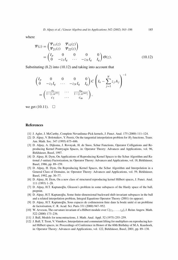
where

�(z) =(

�11(z) �12(z)

�21(z) �22(z)

)

=(Ip 0 0 0 00 −z1Iq · · · −zNIq Iq

)�(z). (10.12)

Substituting (8.2) into (10.12) and taking into account that

(Ip 0 0 0 00 −z1Iq · · · −zNIq Iq

)C

In −

N∑j=1

zjAj

−1

=( a1

1−〈z,w(1)〉 · · · am1−〈z,w(m)〉

c1 · · · cm

),

we get (10.11). �

References

[1] J. Agler, J. McCarthy, Complete Nevanlinna–Pick kernels, J. Funct. Anal. 175 (2000) 111–124.[2] D. Alpay, V. Bolotnikov, Y. Peretz, On the tangential interpolation problem forH2 functions, Trans.

Am. Math. Soc. 347 (1995) 675–686.[3] D. Alpay, A. Dijksma, J. Rovnyak, H. de Snoo, Schur Functions, Operator Colligations and Re-

producing Kernel Pontryagin Spaces, in: Operator Theory: Advances and Applications, vol. 96,Birkhäuser, Basel, 1997.

[4] D. Alpay, H. Dym, On Applications of Reproducing Kernel Spaces to the Schur Algorithm and Ra-tional J -unitary Factorization, in: Operator Theory: Advances and Applications, vol. 18, Birkhäuser,Basel, 1986, pp. 89–159.

[5] D. Alpay, H. Dym, On Reproducing Kernel Spaces, the Schur Algorithm and Interpolation in aGeneral Class of Domains, in: Operator Theory: Advances and Applications, vol. 59, Birkhäuser,Basel, 1992, pp. 30–77.

[6] D. Alpay, H. Dym, On a new class of structured reproducing kernel Hilbert spaces, J. Funct. Anal.111 (1993) 1–28.

[7] D. Alpay, H.T. Kaptanoglu, Gleason’s problem in some subspaces of the Hardy space of the ball,preprint.

[8] D. Alpay, H.T. Kaptanoglu, Some finite-dimensional backward shift-invariant subspaces in the balland a related interpolation problem, Integral Equations Operator Theory (2001) (to appear).

[9] D. Alpay, H.T. Kaptanoglu, Sous espaces de codimension finie dans la boule unité et un problèmede factorisation, C. R. Acad. Sci. Paris 331 (2000) 947–952.

[10] W. Arveson, The curvature invariant of a Hilbert module over C[z1, . . . , zd ], J. Reine Angew. Math.522 (2000) 173–236.

[11] J. Ball, Models for noncontractions, J. Math. Anal. Appl. 52 (1975) 255–259.[12] J. Ball, T. Trent, V. Vinnikov, Interpolation and commutant lifting for multipliers on reproducing ker-

nel Hilbert spaces, in: Proceedings of Conference in Honor of the 60th Birthday of M.A. Kaashoek,in: Operator Theory: Advances and Applications, vol. 122, Birkhäuser, Basel, 2001, pp. 89–138.


[13] M.-J. Bertin, A. Decomps-Guilloux, M. Grandet-Hugot, M. Pathiaux-Delefosse, J.-P. Schreiber,Pisot and Salem Numbers, Birkhäuser, Basel, 1992 (with a preface by David W. Boyd).

[14] L. de Branges, J. Rovnyak, Square Summable Power Series, Holt, Rinehart & Winston, New York,1966.

[15] C. Chamfy, Fonctions méromorphes sur le cercle unité et leurs séries de Taylor, Ann. Inst. Fourier8 (1958) 211–251.

[16] E. Deprettere, P. Dewilde, The Generalized Schur Algorithm, in: Operator Theory: Advances andApplications, vol. 29, Birkhäuser, Basel, 1988, pp. 97–115.

[17] H. Dym, J Contractive Matrix Functions, Reproducing Kernel Hilbert Spaces and Interpolation,Published for the Conference Board of the Mathematical Sciences, Washington, DC, 1989.

[18] D. Greene, S. Richter, C. Sundberg, The structure of inner multipliers on spaces with completeNevanlinna–Pick kernels, preprint.

[19] R. Leech, Factorization of analytic functions and operator inequalities, unpublished manuscript,available at: http://www.people.virginia.edu/∼jlr5m/papers/leech.ps.

[20] S. McCullough, T.T. Trent, Invariant subspaces and Nevanlinna–Pick kernels, preprint.[21] G. Misra, Pick–Nevanlinna interpolation theorem and multiplication operators on functional Hilbert

spaces, Integral Equations Operator Theory 14 (6) (1991) 825–836.[22] R. Nevanlinna, Über beschränkte Funktionen, die in gegebenen Punkten vorgeschriebene Werte

annehmen, Ann. Acad. Sci. Fenn. 1 (1919) 1–71.[23] P. Quiggin, For which reproducing kernel Hilbert spaces is Pick’s theorem true?, Integral Equations

Operator Theory 16 (1993) 244–266.[24] M. Rosenblum, J. Rovnyak, Hardy Classes and Operator Theory, Birkhäuser, Basel, 1985.[25] J. Rovnyak, Characterization of spaces H(M), unpublished manuscript, available at:

http://www.people.virginia.edu/∼jlr5m/papers/HM.ps.[26] W. Rudin, Function Theory in the Unit Ball of Cn, Springer, Berlin, 1980.[27] D. Sarason, Exposed Points in H 1, I, in: Operator Theory: Advances and Applications, vol. 41,

Birkhäuser, Basel, 1989, pp. 485–496.[28] D. Sarason, Exposed Points in H 1, II, in: Operator Theory: Advances and Applications, vol. 48,

Birkhäuser, Basel, 1990, pp. 333–347.[29] I. Schur, Über die Potenzreihen, die im Innern des Einheitkreises beschränkten sind, I, J. Reine

Angew. Math. 147 (1917) 205–232. I. Schur Methods in Operator Theory and Signal Processing, in:Operator Theory: Advances and Applications, vol. 18, Birkhäuser, Basel, 1986 (English translation).

Documents

The Schur algorithm and reproducing kernel Hilbert …kaptan/Files/schur.pdf · Linear Algebra and its ... The Schur algorithm and reproducing kernel Hilbert spaces in the ... Pick