Jz

NASA-CR-ZO1052 _-_

Research Institute for Advanced Computer ScienceNASA Ames Research Center

Learning In Networks

Wray L. Buntine

RIACS Technical Report 95.08April 1995

Invited paper 50th Session of the International Statistical Institute, Beijing, China, August, 1995

https://ntrs.nasa.gov/search.jsp?R=19960026758 2018-09-11T03:00:12+00:00Z

Learning In Networks

Wray L. Buntine

The Research Institute for Advanced Computer Science is operated by Universities Space ResearchAssociation, The American City Building, Suite 212, Columbia, MD 21044 (410) 730-2656

Work reported herein was supported by NASA via Contract NAS 2-13721 between NASA and theUniversities Space Research Association (USRA). Work performed at the Research Institute for AdvancedComputer Science (RIACS), NASA Ames Research Center, Moffett Field, CA 94035-1000

DRAFT Invited paperfor 50th Sessionof the InternationalStatisticalInstitute, Beijing, China,August,1995.

LEARNING IN NETWORKS

Wray L. Buntine

RIACS at NASA Ames Research Center

Mail Stop 269-2

Moffett Field, CA 94035-1000, USA

wray©kronos, arc. nasa. gov

Abstract

Intelligent systems require software incorporating probabilistic reasoning, and often

times learning. Networks provide a framework and methodology for creating this kind

of software. This paper introduces network models based on chain graphs with deter-

ministic nodes. Chain graphs are defined as a hierarchical combination of Bayesian and

Markov networks. To model learning, plates on chain graphs are introduced to model

independent samples. The paper concludes by discussing various operations that can

be performed on chain graphs with plates as a simplification process or to generate

learning algorithms.

Un systeme intelligent doit necessairement inclure un module de raisonement prob-

abiliste et meme bien souvent des mechanismes d'apprentissage. Les reseaux offrent un

cadre et une methodologie pour creer de tels logiciels. Ce papier introduit des modeles

de reseaux bases sur les graphes en chaine avec noeuds deterministes. Un graphe en

chaine est defini comme etant une combinaison hierarchique de reseaux Bayesiens et de

reseaux de Markov. Afin de modeliser l'apprentissage, j'introduit des couches dans ces

graphes en chaines pour modeliser des echantillons independants. Le papier conclue en

discutant un certain nombre d'operations qui peuvent etre effectuees sur les graphes

en chaine afin de les simplifier ou pour generer des algorithmes d'apprentissage.

1 Introduction

This paper introduces a number of network models based on chain graphs. Chain graphs

are a graphical representation including Bayesian networks and Markov networks, which

can represent Markov chains and random Markov fields respectively. The paper also shows

how basic probability calculations including likelihood and Bayesian calculations can be

performed on network models, often times automatically. This collection of models and

tools is intended as a theoretical basis for software supporting probabilistic analysis. This

software perspective is the main driving force for this research, so I spend some time below

introducing it.

Computer scientistsand programmersincreasinglydevelopcomplex softwaresolutionsto intelligent taskssuchas expert systems,speechand natural languageunderstanding,vi-sion, knowledgediscovery,automatic text indexing, robotics, imagematching and indexing,imageclustering and classification, systemsmonitoring, health managementand diagnosis,scientific instrumentation, applied physics,and so forth. Thesetasks involve a high degreeof uncertainty, and henceembeddedprobabilistic reasoning(Heckerman,Mamdani, & Well-man, 1995). Often times, the techniquesneedadaptation using learning from data as well.The needfor a probabilistic approachin someapplications is not obvious from the outset.Considernatural languageunderstanding,usefulfor documentsummarization,classification,and translation. In early artificial intelligence,deterministic grammarswere usedand onlymore recentlyhaveprobabilistic methods takena major role. As another example,only justrecently havecomputer scientistscometo realizethat probabilities canbean important toolfor debuggingsoftware(Burnell & Horvitz, 1995).

Softwarefor intelligent systemsis sufficiently complexthat prototype-refinementcyclesare used rather than a single design-implementationstage. This style of implementationrequires three different skill sets: computer programming, the applications background,and probabilistic techniques. Thesecan only be routinely practiced together in industryif methodologiesand softwareare availablewhich the practitioner cangraspwithout under-going an eight year combinedPhD program. Becauseof a shortagefor computer scientistsof tools and training in the third skill set, probabilistic techniques,many new engineeringand computational styles have arisen to fill the perceivedvoid. Thesenew styles includeneural networks, fuzzy logic, genetic programming, machine learning, and non-monotonicreasoning,somehaving shownsignificant application successes.While many of us believethat computational probabilistic methods well suite intelligent tasks for a variety of appli-cations, the necessarymethodologiesand softwareare not now availablefor engineersanddevelopers.There is an enormousdifferencebetween

• a hand-workedsolution to a oneoff problem in intelligent reasoning,

• a methodological framework for computational probabilistic methods that engineersand other practitioners can be trained in, and

• an automated computationally efficient softwaresolution to a broadly defined familyof problems.

The motivation for this paper is that network methodsprovide the theoretical basisfor thispracticing methodologyand accompanyingefficientsoftware.Thereforenetwork methodsarea critical resourceif we wish to scaleup the production of embeddedprobability softwarefrom the subject of isolated researchto widespreadindustry practice.

As an exampleof this kind of development,my field of researchis data analysis, andI am one of many computer scientistsperforming this task for the reasonsoutlined above.Unfortunately, most of the tasks I seedo not fit into oneof the standard statistical recipes,suchasclustering or non-linear regression,for which excellent softwareis available. Similarnon-standardexamplesfrom medicineare describedin (Gilks, Clayton, Spiegelhalter,Best,

2

McNeil, Sharpies,& Kirby, 1993). Aviation safety data is relational rather than tabularbecauseit has groups of pilots and groupsof aircraft in a singleevent (Kraft & Buntine,1993). Analyzing high resolution spectral data requiresone-dimensionalsuper-resolutiontoestimate the responsefunction for the instrument. Superresolution on this problem is an in-tegrated combination of registration, scaling,and onedimensionalcurve-fitting. Subsequentspectral analysisrequiresprinciple componentsanalysiswheresomenon-orthogonalmetalliccomponentswereobtainedseparatelyfrom ananalytic modelof physicalchemistry (Buntine,Kraft, Whitaker, Cooper,Powers,& Wallace, 1993).Theseproblemsareall non-trivial vari-ations of well known techniques,and thereforerequiresomeadditional programming--evenin a statistically savvy languagesuchasS (Becket, Chambers,& Wilks, 1988).Our budgetin generaldoesnot allow for it. The analysiswaseither not doneor kludged together in anunsatisfactory fashionusing existing tools.

Perhapsthis observation--that data analysisproblemsin generaloften requirenew algo-rithms or carefulmodification of existing algorithms--is well acceptedin statistics. However,

most available software does not support this flexible kind of analysis to the degree that it

could. Of course, one can argue that C or even assembler language can address these kinds

of statistical programming. When we look at the usual budgetary constraints and the back-

ground of the research programmer available for these tasks, most available software is not

adequate. An environment like S does not address the problem directly--many data analysis

algorithms for S are written in C and linked in at runtime. The promise of software sup-

port for data analysis is illustrated by the BUGS software for Bayesian analysis using Gibbs

sampling (Thomas, Spiegelhalter, & Gilks, 1992). This software is a program generator: it

allows a Gibbs sampler to be generated from a model specification.

Software application and support for probability methods is the kind of area that the

relatively new field of probabilistic networks is aimed at serving. The techniques used are

sometimes little more than clever repetition of Bayes theorem. While traditional statistics

grew out of the need to help experimental scientists become "objective" in their reporting

of results, this new field is more concerned with supporting the embedding of probabilistic

reasoning within a larger computational task. In contrast, traditional software developed

by statisticians, for instance, the environments SAS and S largely serve as frameworks to

help statisticians in their sought-after role of analyzing experimental results and other data.

Probabilistic networks are therefore a major paradigmatic shift in focus for the community

with a potentially broad impact: the production of intelligent systems for walking, talking,

seeing and doing, and broad computational support for scientists.

This paper is organized as follows. Chain graphs are motivated and defined in Section 2.

Chain graphs are defined as a composition of directed and undirected networks. Then

deterministic nodes in chain graphs are discussed in Section 3. Deterministic nodes are

important to model constructs such as the linear component of a generalized linear model,

or the sigmoid units of a neural network. Samples are represented on a network using the

notation of plates, described in Section 5. The paper closes by giving some examples of

operations on networks that can be used to simplify a problem, and generate software for

particular key tasks in a learning algorithm. This demonstrates my main point: networks

are a central technologyfor rapid prototyping of learning applications.

2 Probabilistic networks and chain graphs

Probabilistic networks are a notational device that allow one to abstract forms of probabilistic

reasoning without getting lost in the mathematical detail of the underlying equations. They

offer a framework whereby many forms of probabilistic reasoning can be combined and

performed on probabilistic models without careful hand programming. Efforts to date have

largely focused on first-order probabilistic inference, for instance found in expert systems and

diagnosis (Spiegelhalter, Dawid, Lauritzen, &: Cowell, 1993; Heckerman, 1991), and planning

and control (Dean _z Wellman, 1991). For instance, given a set of observations about a

patient, what are the posterior probabilities for different diseases? Should an additional

expensive diagnostic test be performed on the patient? This paper presents methods for

extending techniques on probabilistic networks to handle second-order or statistical problems

and learning, which are concerned with building or improving a probabilistic network from

a database of cases. Second-order inference on probabilistic networks was first suggested

by Lauritzen and Spiegelhalter (Lauritzen _ Spiegelhalter, 1988), and has subsequently

been developed by several groups (Shachter, Eddy, & Hasselblad, 1990; Gilks, Thomas, &

Spiegelhalter, 1993b; Dawid _ Lauritzen, 1993; Buntine, 1994).

This paper uses chain graphs (Wermuth _: Lauritzen, 1989) as a general probabilistic

network model. Chain graphs mix undirected and directed graphs (or networks) to give a

probabilistic representation that includes Markov random fields and various Markov models.

Chain graphs can represent many well known models as a special case including linear and

logistic regression, various forms of clustering, feed-forward neural networks and various

stochastic neural networks. This includes a large number of the more general network models

now available (Ripley, 1994). These many different models are formed by combining basic

nodes in the network representing for instance, Gaussian variables, wavelet basis functions,

or deterministic Sigmoid units. The framework of chain graphs offers a specification language

for defining probabilistic models, and thus the input to a computer program.

In this paper, I define a chain graph as a Bayesian (directed) network whose components

are Bayesian and Markov (undirected) networks. This form of definition allows the complex

independence properties and functional form of a chain graph (Frydenberg, 1990) to be

read off from knowledge of the simpler corresponding properties for directed and undirected

networks. It also allows nodes to be deterministic. First, consider directed and undirected

networks individually, as for instance introduced in (Pearl, 1988; Whittaker, 1990).

2.1 Directed networks

A Bayesian or directed network consists of a set of variables X and a directed graph defined

on it consisting of a node corresponding to each variable and a set of directed arcs. Nodes

in the graph and the variables they represent are used interchangeably. The graph is such

that it contains no directed cycles. In this paper, a directed network defines a particular

4

functional form for the probability distribution p(X) over the variables. Each variable is

written conditioned on its parents, where parents(z) is the set of variables with a directed

arc into x. The general form for this equation for a set of variables X is:

p(X) = 1"I P(xlparents(x))" (1)xEX

This functional form is the interpretation of a directed network used in this paper. The

lemma below shows that this definition is equivalent to a definition based in independence

statements (Lauritzen, Dawid, Larsen, & Leimer, 1990), related to (Pearl, 1988), with the

notation due to (Dawid, 1979).

Definition 1 A is independent of B given C, denoted A BIC, when p(A U BIC) =

p(AIC)p(BIC) for all instantiations of the variables A, B, C.

The following definitions are used here.

Definition 2 The ancestral set, ancestors(A), of a subset A of variables X is the transitive

closure of the relation, f(B) = BUparents(B). The moralized graph G TM of a directed graph

G is formed by making all arcs in G undirected and then connecting each two parents with a

common child in G by adding an additional undirected arc.

The particular independence statements are based on set separation in the moralized graph,

which is equivalent to another condition known as d-separation (Pearl, 1988):

Definition 3 The distribution p(X) satisfies the directed global Markov property relative

to the directed graph G if AlIBIS when S separates A and B in the graph H m where H is

the subgraph of G restricted to ancestors( A tO B tO S).

Lemma 1 Given a directed graph G on X, and A, B, S E X. The distribution p(X) satisfies

the directed global Markov property relative to G if and only if Equation (I) holds.

Given a directed graph, we can therefore read off both the functional decomposition of

Equation (1) and the independence properties easily.

2.2 Undirected networks

Similarly, a Markov or undirected network is an undirected graph on a set of variables

X representing a probability distribution p(X) over the variables. This is analogous to

Lemma 1, except that p(X) must now be strictly positive. The appropriate independence

conditions are based on set separation.

Definition 4 The distribution p(X) satisfies the global Markov property relative to the

undirected graph G if A-U-BIS when S separates A and B in the graph G.

The neighbors for a node x, denoted neighbors(x) are the set of variables directly connected

by an undirected arc to x. An important concept is the set of cliques on the graph.

5

Definition 5 The set of maximal cliques on G is Cliques(G) C 2 x contains all those sets

whose variables are fully connected in G, but none of their strict subsets.

Theorem 1 An undirected graph G is on variables in the set X. The distribution p(X)

is strictly positive in the domain X_xdomain(x). Then the distribution p(X) satisfies the

global Markov property if and only if p(X) satisfies the equation

p(X) : 1-I fc(c), (2)C6Cliques(G)

for some functions fc > O.

The proof follows directly from (Frydenberg, 1990; Buntine, 1994). A form of this theorem

for finite discrete domains is called the Hammersley-Clifford Theorem (Geman, 1990; Besag,

York, & Mollie, 1991). Again, Equation (2) is used as the interpretation of an undirectednetwork.

2.3 Conditional networks

Networks can also represent conditional probability distributions. Conditional networks are

represented by introducing shaded variables in the graph. Shaded variables are assumed to

have their values known, so the probability defined by the network is now conditional on

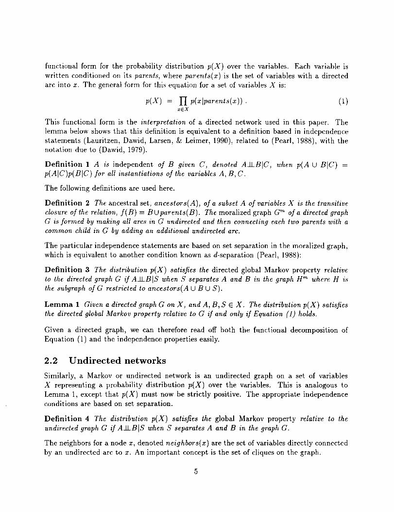
the shaded variables. Figure 1 shows two conditional versions of a simple medical problem

(Shachter & Heckerman, 1987). If the shading of nodes is ignored, the joint probability,

Figure 1: Two equivalent conditional models of the medical problem

p(Age, Occ, Clim, Dis, Syrup) for the two graphs (a) and (b) respectively is:

p( Age) p( OcclAge ) p( ClimlAge, Occ) p( DislAge, Occ, Clim ) p( SymplAge, Dis)

p( Age) p(Occ) p( C tim) p( DislAge, Occ, C lira) p( SymplAge , Dis ).

However, because four of the five nodes are shaded, this means their values are known.

The conditional distributions for p(DislAge , Oce, Clim, Syrup) computed from the above

are identical. When networks contain shaded variables, it is implicit that the distribution

being represented is conditioned on the shaded variables, and therefore, in some cases, some

arcs between shaded variables may be irrelevant.

6

2.4 Chain graphs

In general, a chain graph can be represented as a directed network whose components are

themselves conditional directed or undirected networks. A chain graph is a graph consisting

of mixed directed and undirected arcs, where there are no cycles (of directed and undirected

arcs) whose directed arcs are all in the one direction. The chain graph is first broken up into

component subgraphs as follows.

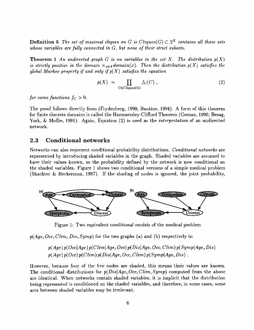
Definition 6 Given a chain graph G over some variables X. The chain components (Fry-

denberg, 1990) are a mutually exclusive and exhaustive partition of X where each element

of the partition is a maximal, connected, undirected subgraph in the chain graph G. The

component subgraphs are a coarser partition of the chain components, where each element

of the partition is a maximal, connected, undirected or directed (but not mixed) subgraph in

the chain graph G. Let chain-components(A) denote all nodes in the same chain componentas at least one variable in A.

Notice that a connected directed graph only has one component subgraph, the graph itself.

Likewise, an undirected graph has each of its connected subgraphs as component subgraphs.

This makes the component subgraphs a natural decomposition of the chain graph into its

maximal directed and undirected parts.

An example is given in Figure 2. Figure 2(a) shows the original chain graph. The chain

(al( (b)

Figure 2: Decomposing a chain graph into its component subgraphs

components of G are {a,b}, {c}, {d}, and {e,f,g,h}. The component subgraphs are formed

by merging c and d into a directed graph. Figure 2(b) shows the directed and undirected

components together with the Bayesian network on the right showing how they are pieced

together. These networks also include some known nodes, to represent conditional networks.

Informally, a chain graph over variables X with component subgraphs given by the set

T is interpreted first as the decomposition corresponding to:

p(X) = 1"I P(rlparents(r)) " (3)vET

The conditional probability p(rlparents(r)) for each component subgraph is now defined

using the corresponding conditional directed or undirected network.

This decompositioncanbe formalizedto givea definition for the interpretation of a chaingraph.

Definition 7 Given a chain graph G on variables X with no given nodes. Let U1,..., Uc

be the component subgraphs of G. Construct a matching set of subgraphs G1,...,Gc as

follows. Let Gi be the subgraph induced by G on Ui U parents(Ui). Then, make the variables

in parents(Ui) all be shaded in Gi and add extra arcs to make parents(Ui) into a clique

(see (Buntine, 1994, Laminas 2.1,2.2)for simplifications to these). Now construct a directed

graph GM whose nodes are U1,..., Uc and arcs connect Ui to Uj if a variable in Ui has a

child in Uj in the graph G. Then the chain graph G is defined to be equivalent to the set of

subgraphs G1, . . . , Gc together with the master graph GM.

One advantage of this formulation is that only undirected component subgraphs need have

the condition of positivity on their conditional distribution, required for Theorem 1 to hold.

Deterministic variables are common in neural networks, and network representations of lo-

gistic or linear regression. Thus, it is important to allow nodes that do not require the

condition of positivity. Some examples of networks with deterministic nodes are given later.

The global Markov property for chain graphs is identical to the directed global Markov

property. This requires that a chain graph be moralized.

Definition 8 The ancestral set for a chain graph, ancestors(A), of a subset A of variables

X is the transitive closure of the relation, f(S) = S U neighbors(B) U parents(B). The

moralized graph G m of a chain graph G is formed by making all arcs in G undirected and

then connecting each two parents with an undirected arc if they both have a child occurring

in the same chain component of G.

The corresponding relationship between independence and the functional form of the prob-

ability distribution then follows directly from Lemma 1 and Theorem 1.

Theorem 2 A chain graph G is on variables in the set X. For every U C X an undi-

rected chain component of G with cardinality greater than I, the conditional distribution

p(Ulparents(U)) is strictly positive in the domain X,_evdomain(x ). Then the distribution

p(X) satisfies the global Markov property for chain graphs if and only if p(Z) satisfies Equa-

tions (1) and (2) for each of its subgraphs and master graph.

3 Deterministic nodes in chain graphs

The previous definitions of a chain graph have been carefully set up to allow nodes to

represent deterministic variables. Consider linear regression where the Gaussian error has a

standard deviation that itself is a function of the inputs, a form of heterogeneous regression.

The probabilistic model of Figure 3(a) gives this model built up from simple nodes that

would be readily available in our network-based software toolkit. Notice how similar this is

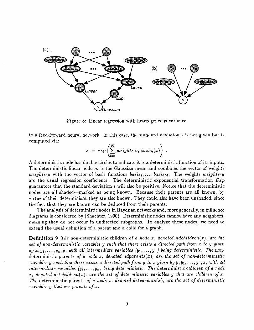
ussian

Figure 3: Linear regression with heterogeneous variance

to a feed-forward neural network. In this case, the standard deviation s is not given but is

computed via:

s = exp weights-ai basisi(x

A deterministic node has double circles to indicate it is a deterministic function of its inputs.

The deterministic linear node rn is the Gaussian mean and combines the vector of weights

weights-# with the vector of basis functions basisl,..., basisM. The weights weights-#

are the usual regression coefficients. The deterministic exponential transformation Exp

guarantees that the standard deviation s will also be positive. Notice that the deterministic

nodes are all shaded--marked as being known. Because their parents are all known, by

virtue of their determinism, they are also known. They could also have been unshaded, since

the fact that they are known can be deduced from their parents.

The analysis of deterministic nodes in Bayesian networks and, more generally, in influence

diagrams is considered by (Shachter, 1990). Deterministic nodes cannot have any neighbors,

meaning they do not occur in undirected subgraphs. To analyze these nodes, we need to

extend the usual definition of a parent and a child for a graph.

Definition 9 The non-deterministic children of a node x, denoted ndchildren(x), are the

set of non-deterministic variables y such that there exists a directed path from x to y given

by x, yl, . . . , y,_ , Y, with all intermediate variables (yl , . . . , y,_) being deterministic. The non-

deterministic parents of a node x, denoted ndparents(x), are the set of non-deterministic

variables y such that there exists a directed path from y to x given by y, yl,..., yn, x, with all

intermediate variables (yl,..., y,_) being deterministic. The deterministic children of a node

x, denoted detchildren(x), are the set of deterministic variables y that are children of x.

The deterministic parents of a node x, denoted detparents(x), are the set of deterministic

variables y that are parents of x.

For instance, in the model in Figure 3(a), the only non-deterministic child of xl is y, and

the deterministic children of xl is basis1,..., basisM. Also notice that for a graph with no

deterministic nodes, ndparents(x) = parents(x) for all nodes x in the graph.

Deterministic nodes can be removed from a graph by rewriting the equations represented

into the remaining variables of the graph. This goes as follows:

Lemma 2 A chain graph G with nodes X has deterministic nodes Y C X and known nodes

K, where K N Y = O. The chain graph G t is created by adding to G a directed arc from

every node to its non-deterministic children, and by deleting the deterministic nodes Y. The

probability models p(X - YIK) satisfying graphs G and G' are equivalent.

An application of this lemma to the chain graph in Figure 3(a) is given in Figure 3(b). You

may observe that for this chain graph, not only is K A Y :p 0, so the conditions of the

lemma do not hold, but in fact K = Y. As noted early, we can equally well mark all the

deterministic nodes unshaded because their non-deterministic parents are all shaded, so this

problem is side stepped.

An important notion used in partitioning graphical models into independent subsets is

the Markov blanket (Pearl, 1988). I use the term Markov boundary here. The Markov

boundary defines the region of local dependence for a node. To split a graphical model

into its independent subgraphs, we then take the transitive closure of the Markov boundary

relation. We introduce an extension here that applies to chain graphs with deterministicnodes.

Definition 10 We have a chain graph G. The Markov boundary of a node u is all neighbors,

non-deterministic parents, non-deterministic children, and non-deterministic parents of the

children and their chain components:

Markov-boundary(u) = neighbors(u) U ndparents(u) t2 ndchildren(u)

tO ndparents( chain-components( ndchildren( u ) )) .

The Markov boundary of a set U is the union of the Markov boundaries for its elements

minus itself.

Markov-boundary(U) = [.J Markov-boundary(u) - U .uEU

From Theorem 2 and Lemma 2 it follows that U is independent of the other non-deterministic

variables in the graph G given its Markov boundary.

Lemma 3 For a chain graph G on variables X, with deterministic nodes D such that U fq

D=0,

U 21_(X - D) lMarkov-boundary(U ) .

What happens when some of the non-deterministic variables in the graph are shaded? Again

from Theorem 2 it follows that the shaded nodes are merely removed from the Markov

boundary.

10

4 Some probabilistic models for unsupervised learn-

ing

las:

Figure 4: Unsupervised learning models

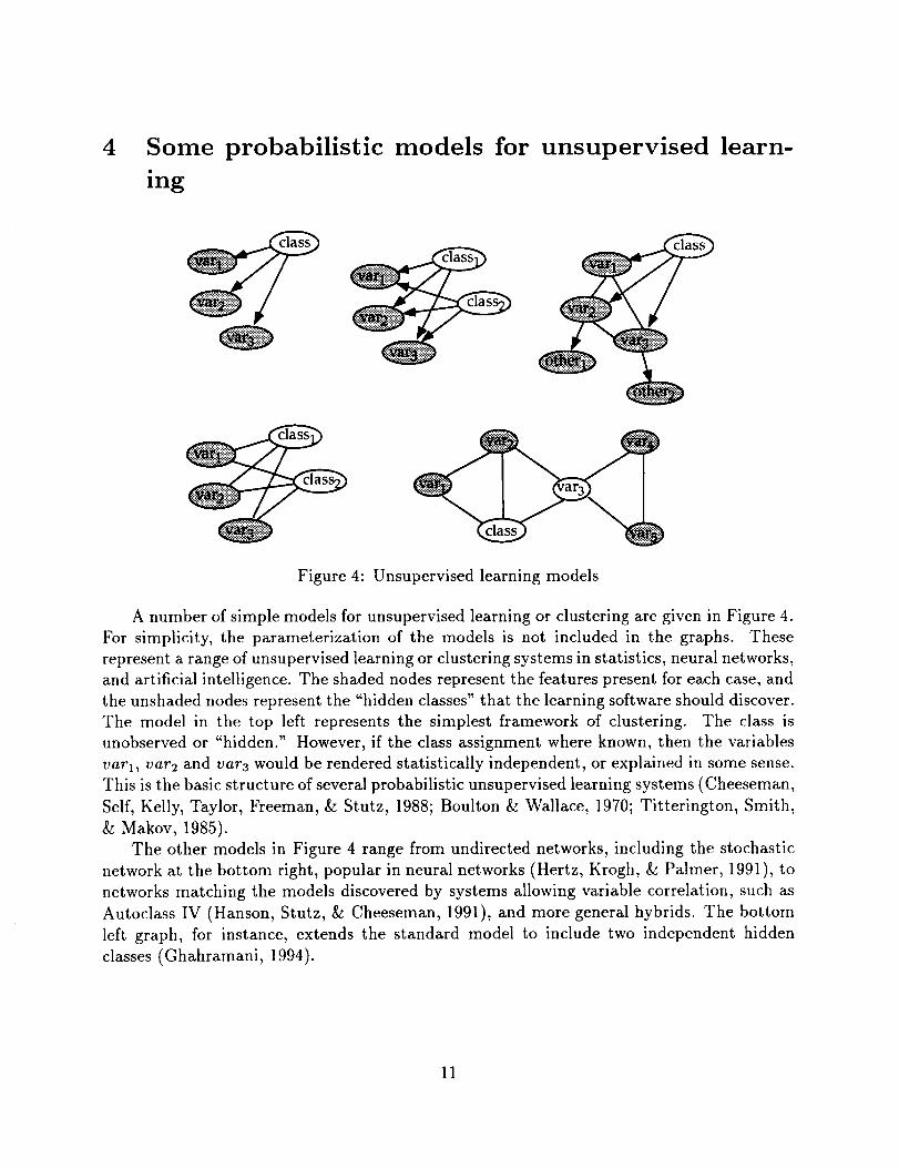
A number of simple models for unsupervised learning or clustering are given in Figure 4.

For simplicity, the parameterization of the models is not included in the graphs. These

represent a range of unsupervised learning or clustering systems in statistics, neural networks,

and artificial intelligence. The shaded nodes represent the features present for each case, and

the unshaded nodes represent the "hidden classes" that the learning software should discover.

The model in the top left represents the simplest framework of clustering. The class is

unobserved or "hidden." However, if the class assignment where known, then the variables

vat1, vat2 and vara would be rendered statistically independent, or explained in some sense.

This is the basic structure of several probabilistic unsupervised learning systems (Cheeseman,

Self, Kelly, Taylor, Freeman, _ Stutz, 1988; Boulton _z Wallace, 1970; Titterington, Smith,

_z Makov, 1985).

The other models in Figure 4 range from undirected networks, including the stochastic

network at the bottom right, popular in neural networks (Hertz, Krogh, _z Palmer, 1991), to

networks matching the models discovered by systems allowing variable correlation, such as

Autoclass IV (Hanson, Stutz, & Cheeseman, 1991), and more general hybrids. The bottom

left graph, for instance, extends the standard model to include two independent hidden

classes (Ghahramani, 1994).

11

5 Chain graphs with plates

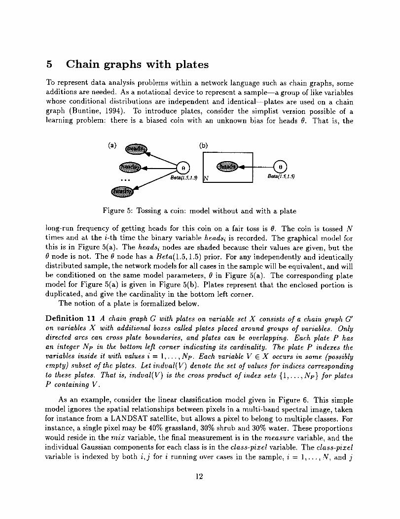
To represent data analysis problems within a network language such as chain graphs, some

additions are needed. As a notational device to represent a sample--a group of like variables

whose conditional distributions are independent and identical--plates are used on a chain

graph (Buntine, 1994). To introduce plates, consider the simplist version possible of a

learning problem: there is a biased coin with an unknown bias for heads 0. That is, the

(a) _ (b)

Figure 5: Tossing a coin: model without and with a plate

long-run frequency of getting heads for this coin on a fair toss is 0. The coin is tossed N

times and at the i-th time the binary variable headsi is recorded. The graphical model for

this is in Figure 5(a). The headsi nodes are shaded because their values are given, but the

0 node is not. The 0 node has a Beta(1.5, 1.5) prior. For any independently and identically

distributed sample, the network models for all cases in the sample will be equivalent, and will

be conditioned on the same model parameters, 0 in Figure 5(a). The corresponding plate

model for Figure 5(a) is given in Figure 5(b). Plates represent that the enclosed portion is

duplicated, and give the cardinality in the bottom left corner.

The notion of a plate is formalized below.

Definition 11 A chain graph G with plates on variable set X consists of a chain graph G'

on variables X with additional boxes called plates placed around groups of variables. Only

directed arcs can cross plate boundaries, and plates can be overlapping. Each plate P has

an integer Np in the bottom left corner indicating its cardinality. The plate P indexes the

variables inside it with values i = 1,..., Np. Each variable V E X occurs in some (possibly

empty) subset of the plates. Let indval(V) denote the set of values for indices corresponding

to these plates. That is, indval(V) is the cross product of index sets {1,..., Np} for plates

P containing V.

As an example, consider the linear classification model given in Figure 6. This simple

model ignores the spatial relationships between pixels in a multi-band spectral image, taken

for instance from a LANDSAT satellite, but allows a pixel to belong to multiple classes. For

instance, a single pixel may be 40% grassland, 30% shrub and 30% water. These proportions

would reside in the mix variable, the final measurement is in the measure variable, and the

individual Gaussian components for each class is in the class-pixel variable. The class-pixel

variable is indexed by both i,j for i running over cases in the sample, i = 1,..., N, and j

12

Dirichlet .. [

_.___mear Gaussian

N

Figure 6: Linear classification model for images

running over classes, j = 1,..., C. Whereas the class means/t are only indexed by j and

the mix is only indexed by i.

5.1 Expanding plates

A graph with plates can be expanded to remove the plates. Figure 5(a) is an expanded form

of Figure 5(b). Given a chain graph with plates G on variables X, construct the expanded

graph as follows:

• For each variable V E X, add a node for Vi for each i E indvar(V).

• For each undirected arc between variables U and V, add an undirected arc between Ui

and V_ for i • indvar(V) = indvar(U).

• For each directed arc between variables U and V, add a directed arc between Ui and

Vj for i • indvar(U) and j • indvar(V) where i and j have identical values for index

components from the same plate if the arc remains inside that plate.

The parents for indexed variables in a graph with plates are the parents in the expanded

graph.

A graph with plates is interpreted using the following product form. The probability

function for the master graph of the chain graph G _ without plates with chain componentsT is

p(XIG') = I'[ p(rlparents(r)),'rET

then for the chain graph G with plates this becomes:

p(XIG) = l'I II p(rilparents(ri)).rET iEindval(_)

(4)

This is given by the expanded version of the graph. Notice these products are over the chain

components and not the component subgraphs--variables in a directed subgraph may occur

in different plates, however, since undirected arcs do not cross plate boundaries, all variables

in the one chain component have identical index sets.

13

5.2 Independence and chain graphs with plates

Testing for independence on chain graphs with plates involves expanding the plates. In

some cases, this can be simplified to an operation on the underlying graph or some simplederivative of it.

For the purposes of modeling learning, however, a critical operation is the partitioning of

a network with plates into its independent subgraphs--each will then be its own independent

learning problem. Given variables X with variables K known (and thus shaded on the graph),

we wish to find the finest partition X1,..., Xm of X - K such that X1 _U_X2-O_ ... _0_XmlK.

By Lemma 3, this problem reduces to finding the finest partition whose elements have empty

Markov boundary. This problem further simplifies because this need only be done for the

graph with plates, not its expanded graph described above. This procedure (Buntine, 1994)

goes as follows. Given a chain graph G with plates on variables X with known variables K.

. Compute the element-wise Markov boundary relation for the graph G ignoring the

plates, and thus compute the finest partition X1,..., Xm. Remember the nodes in K

should be deleted from the computation.

. For each Xi in the partition reproduce its relevant portion of the graph. This means

including any known variables from K n Markov-boundary(Xi) and reproducing all

arcs and plates relevant to these variables.

. The resulting set of graphs is not now the finest partition, but a plate representation

of it. Some sets X_ may have their Markov boundary solely inside a plate, and thus the

plate represents a set of identical but independent subgraphs. This is easily checked

using the Markov boundary.

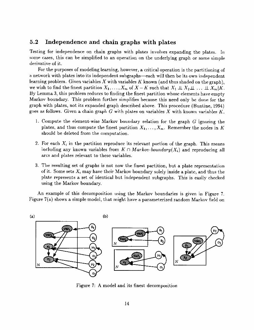
An example of this decomposition using the Markov boundaries is given in Figure 7.

Figure 7(a) shows a simple model, that might have a parameterized random Markov field on

(a) (b)

®N

®

N

Figure 7: A model and its finest decomposition

14

the variablesvarl and var2, and Gaussians on the variables xl and x2. Its decomposition

using the strategy just described is given in Figure 7(b). For instance, in Figure 7(a), the

Markov boundary of {01,02} is the empty set. Therefore, these variables occur in a distinct

subgraph. They cannot be further divided, however, because the Markov boundary of {01}

isAn important gain made by doing a decomposition is that learning can now procede

independently for each of subgraphs. For instance, in Figure 7(b) the Bayes factor (Kass

& Raftery, 1993) for this model versus a null model will take the form of a product over

the subgraphs. In some cases, this allows the search for a MAP model to be improved

considerably (Heckerman, Geiger, & Chickering, 1994), due to an incremental decomposition

(Buntine, 1994).

6 Some useful operations on chain graphs with plates

By defining various operations on chain graphs with plates, such as conditioning and differ-

entiation, useful algorithms can be pieced together for standard statistical procedures such

as maximum likelihood or maximum a posteriori calculations, or the expectation maximiza-

tion algorithm. Chain graphs with plates represent a specification language for data analysis

problems and operations on chain graphs with plates represent the useful subroutines of a

statistical inference system.

In this section, some example subroutines on probabilistic networks are given. Their

intended use is as follows. We would have a software toolkit with various useful network pieces

such as multivariate Gaussians, mixture models, linear modules, and so forth. We plug these

pieces together for a particular novel problem, and then with a few commands, we can split

the problem up into its independent components, reformulate the problem using conjugate

distributions if they exist, and then generate routines for calculating derivatives useful for

MAP calculations or the Laplace approximation (Kass _: Raftery, 1993), or generate sampling

routines for a Gibbs sampler or some other Markov chain Monte Carlo sampler (Neal, 1994,

1993; Gilks et al., 1993b).

6.1 Analysis with conjugate distributions

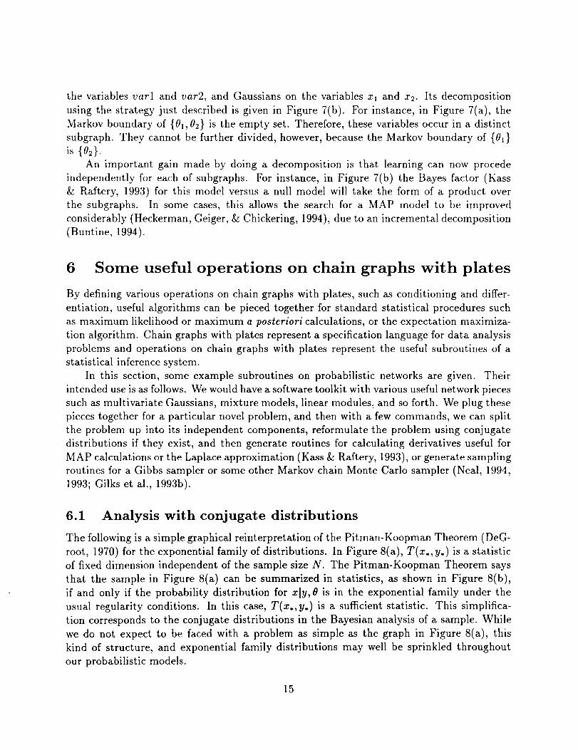
The following is a simple graphical reinterpretation of the Pitman-Koopman Theorem (DeG-

root, 1970) for the exponential family of distributions. In Figure 8(a), T(x., y.) is a statistic

of fixed dimension independent of the sample size N. The Pitman-Koopman Theorem says

that the sample in Figure 8(a) can be summarized in statistics, as shown in Figure 8(b),

if and only if the probability distribution for zig , 0 is in the exponential family under the

usual regularity conditions. In this case, T(x.,y.) is a sufficient statistic. This simplifica-

tion corresponds to the conjugate distributions in the Bayesian analysis of a sample. While

we do not expect to be faced with a problem as simple as the graph in Figure 8(a), this

kind of structure, and exponential family distributions may well be sprinkled throughout

our probabilistic models.

15

(a) (b)

Figure 8: The generalized graph for plate removal

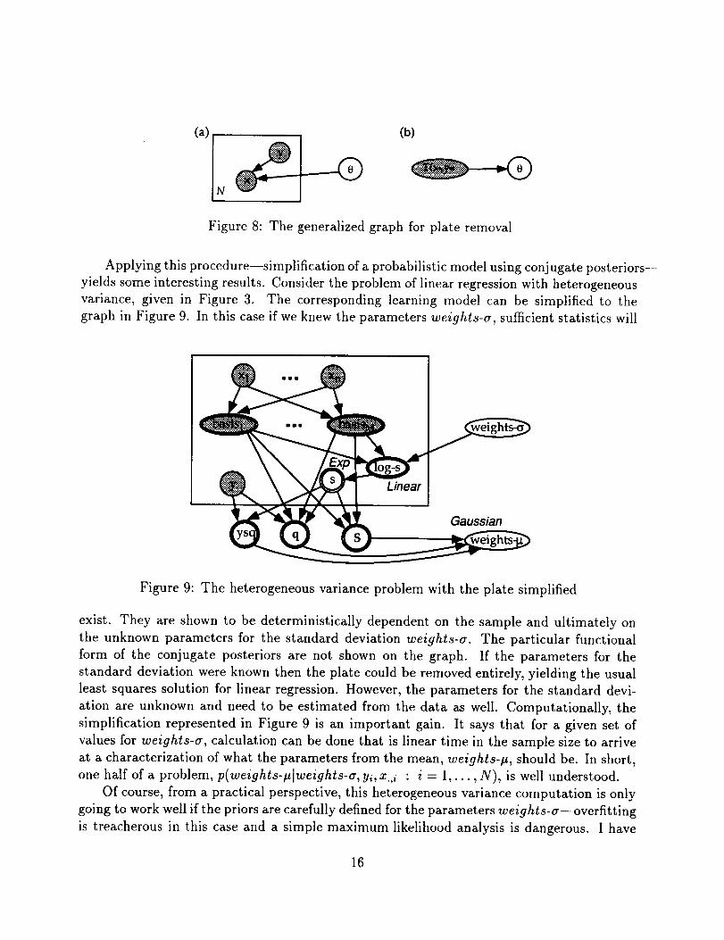
Applying this procedure--simplification of a probabilistic model using conjugate posteriors--

yields some interesting results. Consider the problem of linear regression with heterogeneous

variance, given in Figure 3. The corresponding learning model can be simplified to the

graph in Figure 9. In this case if we knew the parameters weights-a, sufficient statistics will

Gaussian

Figure 9: The heterogeneous variance problem with the plate simplified

exist. They are shown to be deterministically dependent on the sample and ultimately on

the unknown parameters for the standard deviation weights-a. The particular functional

form of the conjugate posteriors are not shown on the graph. If the parameters for the

standard deviation were known then the plate could be removed entirely, yielding the usual

least squares solution for linear regression. However, the parameters for the standard devi-

ation are unknown and need to be estimated from the data as well. Computationally, the

simplification represented in Figure 9 is an important gain. It says that for a given set of

values for weights-a, calculation can be done that is linear time in the sample size to arrive

at a characterization of what the parameters from the mean, weights-#, should be. In short,

one half of a problem, p(weights-#lweights-a , y_, x.,i : i = 1,..., N), is well understood.

Of course, from a practical perspective, this heterogeneous variance computation is only

going to work well if the priors are carefully defined for the parameters weights-a--overfitting

is treacherous in this case and a simple maximum likelihood analysis is dangerous. I have

16

ignored this important point for the purposes of illustration. The benefit of the network

approach is that we can spend more of our time concentrating on getting the priors right,

because part of the effort of algorithm construction will be simplified for us.

6.2 Derivatives of probabilistic networks

An important operation on networks is the calculation of derivatives of parameters. This is

useful after conditioning on the known data to do approximate inference. Numerical opti-

mization (Gill, Murray, & Wright, 1981) using derivatives can be done to search for MAP

values of parameters, or to apply the Laplace approximation to estimate moments. To use

a gradient descent, conjugate gradient or Levenberg-Marquardt approach requires calcula-

tion of first derivatives. To use a Newton-Raphson approach requires calculation of second

derivatives, as well. While this could be done numerically by difference approximations, more

accurate calculations exist. Methods for symbolically differentiating networks of functions,

and piecing together the results to produce global derivatives are well understood (Griewank

& Corliss, 1991). For instance, software is available for taking a function defined in Fortran,

C++ code, or some other language, to produce a second function that computes the exact

derivative. These problems are also well understood for feed-forward networks (Werbos,

McAvoy, & Su, 1992; Buntine & Weigend, 1994), and graphical models with plates only add

some additional complexity. The basic results are discussed in this section and some simple

examples given to highlight special characteristics arising from their use with chain graphs.

Deterministic nodes form islands of determinism within the uncertainty represented by

the network. Partial derivatives within each island can be calculated via recursive use of

the chain rule, for instance, by forward or backward propagation of derivatives through the

equations. For instance, consider Figure 9. There is a single island of determinism here, all

variables except the weights. Forward propagation for this network gives:

Oysq N Oysq Osi

Oweights-a - _ Osi Oweights-a"i----1

Notice that o_e°f_ts _ = 0. These equations recurse forward from _ 0_.o_-s, to eventually- owetgh_s-a

compute the partial derivative for ysq, q and S. In contrast, backward propagation would

propagate derivatives of ysq with respect to different variables backwards. For each island

of determinism, the important variables are the output variables, and their derivatives are

required.

This is nothing more than the chain rule for differentiation, but it is important to notice

the network structure of the computation. When partial derivatives are computed over net-

works, there are local and global partial derivatives that can be different. Local derivatives

are computed for input-output variables local to a node, whereas global derivatives are com-

puted for the entire network. The network structure shows how to combine local derivatives

to form global derivatives. In general, the partial derivative for an index variable Oi is thesum of

17

• the local partial derivative at the node containing 0_,

• the partial derivatives for each child of 0i that is also a non-deterministic child, and

• combinations of (global) partial derivatives for deterministic children found by back-

ward or forward propagation of derivatives.

Therefore, network-based software can be implemented to calculate derivatives of chain

graphs.

7 Conclusion

Networks with a library of useful nodes and generators for routines can provide the soft-

ware environment for creating reliable learning software quickly. This applies to both the

maximum likelihood and Bayesian frameworks for statistical inference. Software for process-

ing networks based on chain graphs should supersede the technologies of generalized linear

models (McCullagh & Nelder, 1989), and many algorithms from neural networks. Of course,

this does not simplify the critical tasks of modelling and choosing appropriate priors for a

problem. These two tasks might be said to be an art form. However, they would become

much easier to handle if underlying, routine, software support was available.

BIBLIOGRAPHY

Becker, R., Chambers, J., & Wilks, A. (1988). The New S Language. Wadsworth &

Brooks/Cole, Pacific Grove, California.

Besag, J., York, J., & Mollie, A. (1991). Bayesian image restoration with two applications

in spatial statistics. Ann. Inst. Statist. Math., 43(1), 1-59.

Boulton, D., & Wallace, C. (1970). A program for numerical classification. The Computer

Journal, 13(1), 63-69.

Buntine, W. (1994). Operations for learning with graphical models. Journal of Artificial

Intelligence Research, 2, 159-225.

Buntine, W., Kraft, R., Whitaker, K., Cooper, A., Powers, W., & Wallace, T. (1993).

OPAD data analysis. In AIAA/SAE/ASME/ASEE 29th Joint Propulsion Conference

Monterey, California.

Buntine, W., _ Weigend, A. (1994). Computing second derivatives in feed-forward networks:

a review. IEEE Transactions on Neural Networks, 5(3).

Burnell, L., & Horvitz, E. (1995). Structure and chance: Melding logic and probability for

software debugging. Communications of the ACM, 37(3).

Cheeseman, P., Self, M., Kelly, J., Taylor, W., Freeman, D., & Stutz, J. (1988). Bayesian

classification. In Seventh National Conference on Artificial Intelligence, pp. 607-611

Saint Paul, Minnesota. American Association for Artificial Intelligence.

18

Dawid, A. (1979). Conditional independencein statistical theory. SIAM Journal on Com-

puting, 41, 1-31.

Dawid, A., & Lauritzen, S. (1993). Hyper Markov laws in the statistical analysis of decom-

posable graphical models. Annals of Statistics, 21(3), 1272-1317.

Dean, T., & Wellman, M. (1991). Plannin 9 and Control. Morgan Kaufmann, San Mateo,California.

DeGroot, M. (1970). Optimal Statistical Decisions. McGraw-Hill.

Frydenberg, M. (1990). The chain graph Markov property. Scandinavian Journal of Statis-

tics, 17, 333-353.

Geman, D. (1990). Random fields and inverse problems in imaging. In Hennequin, P. (Ed.),l_cole d'Et_ de Probabilitgs de Saint-Flour XVIII- 1988. Springer-Verlag, Berlin. In

Lecture Notes in Mathematics, Volume 1427.

Ghahramani, Z. (1994). Factorial learning and the EM algorithm. In Tesauro, G., Touret-

zky, D., & Leen, T. (Eds.), Advances in Neural Information Processing Systems 7

(NIPS*93). Morgan Kaufmann.

Gilks, W., Clayton, D., Spiegelhalter, D., Best, N., McNeil, A., Sharpies, L., & Kirby, A.

(1993a). Modelling complexity: applications of Gibbs sampling in medicine. Journal

of the Royal Statistical Society B, 55, 39-102.

Gilks, W., Thomas, A., & Spiegelhalter, D. (1993b). A language and program for complex

Bayesian modelling. The Statistician, 43, 169-178.

Gill, P. E., Murray, W., & Wright, M. H. (1981). Practical Optimization. Academic Press,

San Diego.

Griewank, A., & Corliss, G. F. (Eds.). (1991). Automatic Differentiation of Algorithms:

Theory, Implementation, and Application, Breckenridge, Colorado. SIAM.

Hanson, R., Stutz, J., & Cheeseman, P. (1991). Bayesian classification with correlation and

inheritance. In IJCAI91 (Ed.), International Joint Conference on Artificial Intelligence

Sydney. Morgan Kaufmann.

Heckerman, D., Geiger, D., & Chickering, D. (1994). Learning Bayesian networks: The com-

bination of knowledge and statistical data. Technical report MSR-TR-94-09 (Revised),

Microsoft Research, Advanced Technology Division. To appear, Machine LearningJournal.

Heckerman, D., Mamdani, A., & Wellman, M. (1995). Real-world applications of Bayesian

networks: Introduction. Communications of the ACM, 38(3).

Heckerman, D. (1991). Probabilistic Similarity Networks. MIT Press.

Hertz, J., Krogh, A., & Palmer, R. (1991). Introduction to the Theory of Neural Computation.

Addison-Wesley.

Kass, R., & Raftery, A. (1993). Bayes factors and model uncertainty. Technical report

#571, Department of Statistics, Carnegie Mellon University, PA. To appear, Journal

of American Statistical Association.

Kraft, R., & Buntine, W. (1993). Initial exploration of the ASRS database. In Seventh

19

International Symposium on Aviation Psychology Columbus, Ohio.

Lauritzen, S., Dawid, A., Larsen, B., & Leimer, H.-G. (1990). Independence properties of

directed Markov fields. Networks, 20, 491-505.

Lauritzen, S., & Spiegelhalter, D. (1988). Local computations with probabilities on graphical

structures and their application to expert systems (with discussion). Journal of the

Royal Statistical Society B, 50(2), 240-265.

McCullagh, P., & Nelder, J. (1989). Generalized Linear Models (second edition). Chapmanand Hall, London.

Neal, R. M. (1994). Bayesian Learning for Neural Networks. Ph.D. thesis, University

of Toronto, Graduate Department of Computer Science. Available via FTP from

ftp ://cs. toronto, edu/pub/radford/thesis .ps.Z.

Neal, R. (1993). Probabilistic inference using Markov chain Monte Carlo methods. Technical

report CRG-TR-93-1, Dept. of Computer Science, University of Toronto.

Pearl, J. (1988). Probabilistic Reasoning in Intelligent Systems. Morgan Kaufmann.

Ripley, B. (1994). Network methods in statistics. In Kelly, F. (Ed.), Probability, Statistics

and Optimization, pp. 241-253. Wiley L; Sons, New York.

Shachter, R. (1990). An ordered examination of influence diagrams. Networks, 20, 535-563.

Shachter, R., Eddy, D., & Hasselblad, V. (1990). An influence diagram approach to medical

technology assessment. In Oliver, R., & Smith, J. (Eds.), Influence Diagrams, Belief

Nets and Decision Analysis, pp. 321-350. Wiley.

Shachter, R., & Heckerman, D. (1987). Thinking backwards for knowledge acquisition. AI

Magazine, 8(Fall), 55-61.

Spiegelhalter, D., Dawid, A., Lauritzen, S., & Cowell, R. (1993). Bayesian analysis in expert

systems. Statistical Science, 8(3), 219-283.

Thomas, A., Spiegelhalter, D., & Gilks, W. (1992). BUGS: A program to perform Bayesian

inference using Gibbs sampling. In Bernardo, J., Berger, J., Dawid, A., & Smith, A.

(Eds.), Bayesian Statistics 4, pp- 837-42. Oxford University Press.

Titterington, D., Smith, A., & Makov, U. (1985). Statistical Analysis of Finite Mixture

Distributions. John Wiley & Sons, Chichester.

Werbos, P. J., McAvoy, T., & Su, T. (1992). Neural networks, system identification, and

control in the chemical process industry. In White, D. A., & Sofge, D. A. (Eds.),

Handbook of Intelligent Control, pp. 283-356. Van Nostrand Reinhold.

Wermuth, N., & Lauritzen, S. (1989). On substantive research hypotheses, conditional

independence graphs and graphical chain models. Journal of the Royal Statistical

Society B, 5I (3).

Whittaker, J. (1990). Graphical Models in Applied Multivariate Statistics. Wiley.

20

RIACSMail Stop T041-5

NASA Ames Research Center

Moffett Field, CA 94035