Embed Size (px)
Citation preview

Learning Econometrics with GAUSS
by
Ching-Fan Chung
Institute of Economics, Academia Sinica
♠ · ♥ · ♦ · ♣

ii

Contents
1 Introduction 11.1 Getting Started with GAUSS . . . . . . . . . . . . . . . . . . . . . . . . . . . . . . . . . .2
1.1.1 Executing DOS Commands in GAUSS . . . . . . . . . . . . . . . . . . . . . . . .31.1.2 Some GAUSS Keystrokes . . . . . . . . . . . . . . . . . . . . . . . . . . . . . . .31.1.3 A Note on Computer Memory . . . . . . . . . . . . . . . . . . . . . . . . . . . . .4
1.2 The GAUSS Editor . . . . . . . . . . . . . . . . . . . . . . . . . . . . . . . . . . . . . . .41.3 GAUSS Statements . . . . . . . . . . . . . . . . . . . . . . . . . . . . . . . . . . . . . . .5
1.3.1 Some Syntax Rules . . . . . . . . . . . . . . . . . . . . . . . . . . . . . . . . . . .61.3.2 Two Types of Errors . . . . . . . . . . . . . . . . . . . . . . . . . . . . . . . . . .6
2 Data Input and Output 92.1 ASCII Files . . . . . . . . . . . . . . . . . . . . . . . . . . . . . . . . . . . . . . . . . . .9
2.1.1 ASCII Data Files . . . . . . . . . . . . . . . . . . . . . . . . . . . . . . . . . . . .102.1.2 ASCII Output Files . . . . . . . . . . . . . . . . . . . . . . . . . . . . . . . . . . .112.1.3 Other Commands Related to ASCII Output Files . . . . . . . . . . . . . . . . . . .122.1.4 An Example . . . . . . . . . . . . . . . . . . . . . . . . . . . . . . . . . . . . . .13
2.2 Matrix Files . . . . . . . . . . . . . . . . . . . . . . . . . . . . . . . . . . . . . . . . . . .15
3 Basic Algebraic Operations 173.1 Arithmetic Operators . . . . . . . . . . . . . . . . . . . . . . . . . . . . . . . . . . . . . .173.2 Element-by-Element Operations . . . . . . . . . . . . . . . . . . . . . . . . . . . . . . . .173.3 Other Arithmetic Operators . . . . . . . . . . . . . . . . . . . . . . . . . . . . . . . . . . .183.4 Priority of the Arithmetic Operators . . . . . . . . . . . . . . . . . . . . . . . . . . . . . .193.5 Matrix Concatenation and Indexing Matrices . . . . . . . . . . . . . . . . . . . . . . . . .20
4 GAUSS Commands 234.1 Special Matrices . . . . . . . . . . . . . . . . . . . . . . . . . . . . . . . . . . . . . . . . .234.2 Simple Statistical Commands . . . . . . . . . . . . . . . . . . . . . . . . . . . . . . . . . .234.3 Simple Mathematical Commands . . . . . . . . . . . . . . . . . . . . . . . . . . . . . . . .244.4 Matrix Manipulation . . . . . . . . . . . . . . . . . . . . . . . . . . . . . . . . . . . . . .244.5 Basic Control Commands . . . . . . . . . . . . . . . . . . . . . . . . . . . . . . . . . . . .254.6 Some Examples . . . . . . . . . . . . . . . . . . . . . . . . . . . . . . . . . . . . . . . . .264.7 Character Matrices and Strings . . . . . . . . . . . . . . . . . . . . . . . . . . . . . . . . .34
4.7.1 Character Matrices . . . . . . . . . . . . . . . . . . . . . . . . . . . . . . . . . . .344.7.2 Strings . . . . . . . . . . . . . . . . . . . . . . . . . . . . . . . . . . . . . . . . .354.7.3 The Data Type . . . . . . . . . . . . . . . . . . . . . . . . . . . . . . . . . . . . .364.7.4 Three Useful GAUSS Commands . . . . . . . . . . . . . . . . . . . . . . . . . . .36
5 GAUSS Program for Linear Regression 415.1 A Brief Review . . . . . . . . . . . . . . . . . . . . . . . . . . . . . . . . . . . . . . . . .41
5.1.1 The Ordinary Least Squares Estimation . . . . . . . . . . . . . . . . . . . . . . . .415.1.2 Analysis of Variance . . . . . . . . . . . . . . . . . . . . . . . . . . . . . . . . . .425.1.3 Durbin-Watson Test Statistic . . . . . . . . . . . . . . . . . . . . . . . . . . . . . .43
5.2 The Program . . . . . . . . . . . . . . . . . . . . . . . . . . . . . . . . . . . . . . . . . .445.3 The ‘ols’ Command . . . . . . . . . . . . . . . . . . . . . . . . . . . . . . . . . . . . . .48
iii

iv CONTENTS
5.4 Linear Restrictions . . . . . . . . . . . . . . . . . . . . . . . . . . . . . . . . . . . . . . .535.5 Chow Test for Structural Changes . . . . . . . . . . . . . . . . . . . . . . . . . . . . . . .55
6 Relational Operators and Logic Operators 596.1 Relational Operators . . . . . . . . . . . . . . . . . . . . . . . . . . . . . . . . . . . . . .596.2 Logic Operators . . . . . . . . . . . . . . . . . . . . . . . . . . . . . . . . . . . . . . . . .606.3 Conditional Statements . . . . . . . . . . . . . . . . . . . . . . . . . . . . . . . . . . . . .606.4 Row-Selectors: the ‘selif’ and ‘delif’ Commands . . . . . . . . . . . . . . . . . . . . .626.5 Dummy Variables in Linear Regression Models . . . . . . . . . . . . . . . . . . . . . . . .62
6.5.1 Binary Dummy Variables . . . . . . . . . . . . . . . . . . . . . . . . . . . . . . . .626.5.2 The Polychotomous Case . . . . . . . . . . . . . . . . . . . . . . . . . . . . . . . .676.5.3 The Piecewise Linear Regression Model . . . . . . . . . . . . . . . . . . . . . . . .71
7 Iteration with Do-Loops 757.1 Do-loops . . . . . . . . . . . . . . . . . . . . . . . . . . . . . . . . . . . . . . . . . . . .757.2 Some Statistics Related to the OLS Estimation . . . . . . . . . . . . . . . . . . . . . . . . .80
7.2.1 The Heteroscedasticity Problem . . . . . . . . . . . . . . . . . . . . . . . . . . . .807.2.2 The Autocorrelation Problem . . . . . . . . . . . . . . . . . . . . . . . . . . . . .827.2.3 Structural Stability . . . . . . . . . . . . . . . . . . . . . . . . . . . . . . . . . . .85
8 GAUSS Procedures: Basics 878.1 Structural Programming . . . . . . . . . . . . . . . . . . . . . . . . . . . . . . . . . . . . .928.2 Accessing Global Variables Directly . . . . . . . . . . . . . . . . . . . . . . . . . . . . . .938.3 Calling Other Procedures in a Procedure . . . . . . . . . . . . . . . . . . . . . . . . . . . .948.4 String Inputs . . . . . . . . . . . . . . . . . . . . . . . . . . . . . . . . . . . . . . . . . . .968.5 Functions: Simplified Procedures . . . . . . . . . . . . . . . . . . . . . . . . . . . . . . . .988.6 Keywords: Specialized Procedures? . . . . . . . . . . . . . . . . . . . . . . . . . . . . . .99
9 GAUSS Procedures: The Library System and Compiling 1019.1 Autoloading and the Library Files . . . . . . . . . . . . . . . . . . . . . . . . . . . . . . .1019.2 The ‘GAUSS.LCG’ Library File for Extrinsic GAUSS Commands . . . . . . . . . . . . . . .1029.3 The ‘USER.LCG’ Library File for User-Defined Procedures . . . . . . . . . . . . . . . . . .1029.4 Other Library Files . . . . . . . . . . . . . . . . . . . . . . . . . . . . . . . . . . . . . . .1029.5 On-Line Help: Seeking Information as the Autoloader . . . . . . . . . . . . . . . . . . . .1039.6 Compiling? . . . . . . . . . . . . . . . . . . . . . . . . . . . . . . . . . . . . . . . . . . .1039.7 The External and Declare Commands . . . . . . . . . . . . . . . . . . . . . . . . . . . . .104
10 Nonlinear Optimization 10710.1 Newton’s Method . . . . . . . . . . . . . . . . . . . . . . . . . . . . . . . . . . . . . . . .107
10.1.1 The Computation of Gradients . . . . . . . . . . . . . . . . . . . . . . . . . . . . .10810.1.2 The Computation of Hessian . . . . . . . . . . . . . . . . . . . . . . . . . . . . . .10910.1.3 Quasi-Newton Method . . . . . . . . . . . . . . . . . . . . . . . . . . . . . . . . .10910.1.4 Newton’s Method for Maximum Likelihood Estimation . . . . . . . . . . . . . . . .11010.1.5 The Computation of the Step Length . . . . . . . . . . . . . . . . . . . . . . . . . .111
10.2 A GAUSS Program for Nonlinear Minimization: NLOPT . . . . . . . . . . . . . . . . . . .11110.2.1 Changing Options . . . . . . . . . . . . . . . . . . . . . . . . . . . . . . . . . . .115

CONTENTS v
10.2.2 Analytic Gradients and Analytic Hessian . . . . . . . . . . . . . . . . . . . . . . .11610.2.3 Imposing Restrictions . . . . . . . . . . . . . . . . . . . . . . . . . . . . . . . . .12010.2.4 Additional Options . . . . . . . . . . . . . . . . . . . . . . . . . . . . . . . . . . .12310.2.5 Run-Time Option Switching . . . . . . . . . . . . . . . . . . . . . . . . . . . . . .12310.2.6 Global Variable List . . . . . . . . . . . . . . . . . . . . . . . . . . . . . . . . . .125
A Drawing Graphs for the Simple Linear Regression Model 300
B GAUSS Data Set (GDS) Files 311B.1 Writing Data to a New GAUSS Data Set . . . . . . . . . . . . . . . . . . . . . . . . . . . .311B.2 Reading the GAUSS Data Set . . . . . . . . . . . . . . . . . . . . . . . . . . . . . . . . . .314
B.2.1 Using Variable Names . . . . . . . . . . . . . . . . . . . . . . . . . . . . . . . . .315B.3 Reading and Processing Data with Do-Loops . . . . . . . . . . . . . . . . . . . . . . . . .315
B.3.1 The ‘readr’ and the ‘writer’ Commands and Do-Loop . . . . . . . . . . . . . . .317B.3.2 The ‘seekr’ Command . . . . . . . . . . . . . . . . . . . . . . . . . . . . . . . . .318
B.4 GAUSS Commands That Are Related to GDS Files . . . . . . . . . . . . . . . . . . . . . .318B.4.1 Sorting the GDS File . . . . . . . . . . . . . . . . . . . . . . . . . . . . . . . . . .319B.4.2 The ‘ols’ Command and the GDS File . . . . . . . . . . . . . . . . . . . . . . . .319
B.5 Revising GDS Files . . . . . . . . . . . . . . . . . . . . . . . . . . . . . . . . . . . . . . .320B.6 Reading and Writing Small GDS Files . . . . . . . . . . . . . . . . . . . . . . . . . . . . .320B.7 The ATOG Program? . . . . . . . . . . . . . . . . . . . . . . . . . . . . . . . . . . . . . .321
B.7.1 The Structure of the Source ASCII file . . . . . . . . . . . . . . . . . . . . . . . . .322

vi CONTENTS

Chapter 1Introduction
GAUSS is a computer programming language. We use it to write programs, i.e., collections of commands.Each command in a GAUSS program directs a computer to do one mathematical or statistical operation.The main difference between the GAUSS language and the other statistics packages is that using GAUSSrequires us to know more about the mathematical derivation underlying each statistical procedure becausewe have to translate it into GAUSS language. The advantage of using a programming language is themaximum flexibility it allows for. There is virtually no limit in what we can do with GAUSS. The maindifference between GAUSS and other programming languages, such as Fortran, C, Pascal, etc. is that thebasic elements for mathematical operations in GAUSS are matrices. This is a powerful feature that can saveus from many programming details and allow us to concentrate more on statistics and econometrics.
Let’s use an example to explain this feature. Consider the following equation:
1 y = X*b + e; /* 1.1 */
If we see equation/* 1.1*/ in an econometrics class, then it is quite natural to associate it with the follow-ing “handwritten” equation:
y = Xβββ + εεε. (1.1)
It is almost like our instinct to think ‘y’ in equation/* 1.1 */ as a column vector, containing observationson the dependent variable, ‘X’ a matrix, containing observations on some explanatory variables, ‘b’ a columnof parameters, and ‘e’ of course a column of error terms.1 In other words, we will interpret equation/* 1.1 */ just like we interpret equation (1.1). The only difference is simply the style: equation (1.1) is ina more elaborated font where Greek letterβββ is used, while equation/* 1.1 */ is written in plain Englishletters. Perhaps we are not so sure about why there is an asterisk ‘*’ between ‘X’ and ‘b’ in /* 1.1 */.But we might just guess that it means matrix multiplication. We may also wonder why in/* 1.1 */ thereis a semicolon after ‘e’ and why the equation number is written in a strange way like/* 1.1 */. Theseand many other questions about styles will be explained fully in the next two chapters. But no matter howstrange we may feel about the expression in/* 1.1 */, the important thing is that we can always guessits meaning while those unusual details generally do not bother us very much. In fact, the interpretationof /* 1.1 */ is so natural that we may wish computers can understand it just like we do. Fortunately,computers do understand it, but only in GAUSS.
GAUSS is a computer language in which expressions are very close to their hand-written counterparts.As a result, GAUSS minimizes our effort to translate a handwritten mathematical expression to a form thatcomputers can understand. To appreciate how much trouble GAUSS has saved us from, we have to knowthe nature of computers. Other than the capability of doing some basic arithmetic in high speed, computersactually are very dumb. We have taken education for years to become what we are now. Computers never
1Whenever elements of a GAUSS program, such as ‘y’, ‘ X’, ‘ b’, ‘ e’, appear in the text, they will be in a special font, that differsfrom the standard text font, and enclosed by single quote ‘ and ’.
1

2 CHAPTER 1. INTRODUCTION
really “learn” anything. Just imagine how difficult it would be to explain things like vectors and matrices toa kindergarten kid. By the same token, to explain the meaning of econometric equations in matrix form tocomputers is not an easy job. For instance, computers need to be informed that a letter like ‘y’ should beunderstood as a mathematical item called vector that follows certain rules. Nevertheless, GAUSS saves usall these troubles. When we write equation/* 1.1 */ in GAUSS, computers will understand it just like theway we want them to.
This book is written for a person who has little knowledge about computer programming to get on withGAUSS as quickly as possible. Every thing in GAUSS is explained from scratch. However, some knowledgeabout DOS, the basic operation system of the IBM-compatible computers, is assumed. GAUSS has gonethrough several editions. The edition we discuss here is GAUSS-386i version 3.2.
1.1 Getting Started with GAUSS
The procedure of using GAUSS is as follows: we first type our GAUSS program in a text file and then submitthis file to a personal computer for processing. Once the computer fully understands what we want to doin the GAUSS program, the program is executed. This process is calledto have a computer run a GAUSSprogram in the edit mode. (There is an alternative way of running a GAUSS program called running it inthe command mode, which is seldom used when the GAUSS program contains more than five statements.)
To type the GAUSS program into a text file, we need a wordprocessor (e.g., WordPerfect, Word, AMI,etc.) or an editor (e.g., the DOS editor, the GAUSS editor, etc.). No matter which wordprocessor or editorwe use, we have to make sure the file we create is a plain ASCII file without anyformatting codes. Word-processor users are especially cautioned here. Almost all wordprocessors embed formatting codes in filesthey create. These formatting codes explain why files created by one wordprocessor cannot be read directlyby other wordprocessors. However, almost all wordprocessors, under some special directions, can createASCII files. So we can use any wordprocessor to write GAUSS programs if we know how to get rid ofthose formatting codes and leave a plain ASCII file. Editors work like scaled-down wordprocessors. Butin general the files created by editors are plain ASCII files. Boththe DOS editorandthe GAUSS editorarequite good for the purpose of typing GAUSS programs and each can be learned in less than half an hour. TheGAUSS editor will be briefly introduced in the next section. (However, for those people who do not want touse the GAUSS editor, that section may be skipped without affecting the continuity of the discussion.)
Once we have finished typing the GAUSS program in an ASCII file with a file name, say,prg.1, wethen submit it for execution. To do this, first we have to go intothe GAUSS environmentfrom the DOSenvironment. That is, under DOS, we type
1 gaussi
after the DOS prompt ‘>’ and press the ‘Enter’ key. A few seconds later, some information about thestatus of GAUSS, such as the size of usable memory, will appear on the screen and we are in the GAUSSenvironment. The GAUSS prompt ‘>>’ will show up on the screen waiting for us to type GAUSS commands.In GAUSS terminology, the GAUSS environment we are in is referred to as the GAUSS command mode.We can directly type GAUSS statements on the screen and execute them (a procedure that is called runningGAUSS in the command mode). But this is not most convenient way to use GAUSS. We should insteadtype a GAUSS program in an ASCII file first and then submit it for execution in the edit mode, as briefly
1.1. GETTING STARTED WITH GAUSS 3
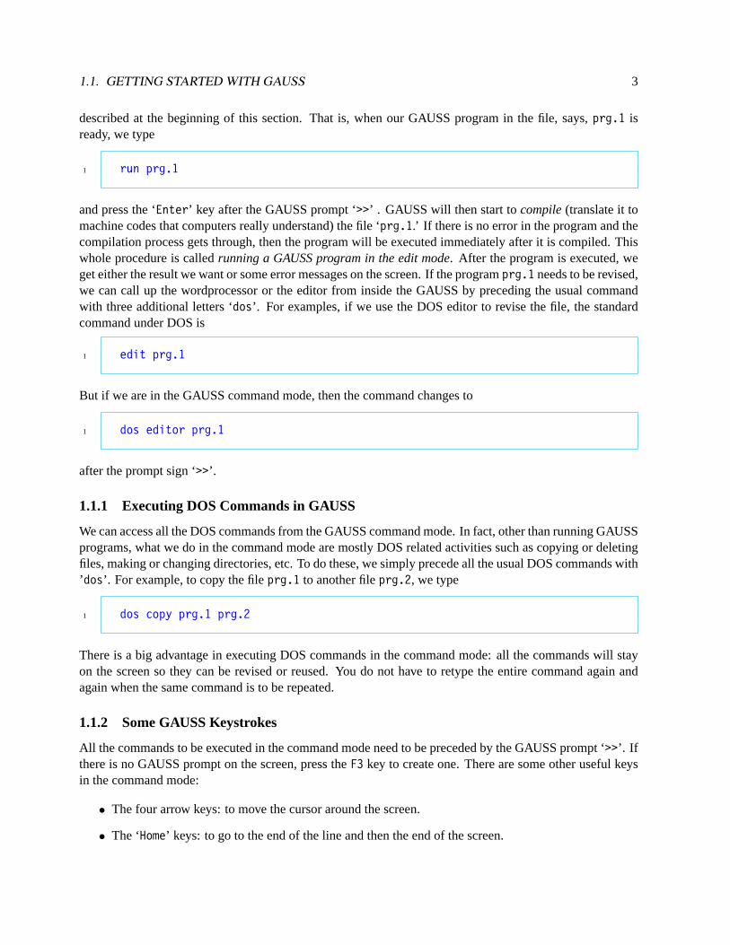
described at the beginning of this section. That is, when our GAUSS program in the file, says,prg.1 isready, we type
1 run prg.1
and press the ‘Enter’ key after the GAUSS prompt ‘>>’ . GAUSS will then start tocompile(translate it tomachine codes that computers really understand) the file ‘prg.1.’ If there is no error in the program and thecompilation process gets through, then the program will be executed immediately after it is compiled. Thiswhole procedure is calledrunning a GAUSS program in the edit mode. After the program is executed, weget either the result we want or some error messages on the screen. If the programprg.1 needs to be revised,we can call up the wordprocessor or the editor from inside the GAUSS by preceding the usual commandwith three additional letters ‘dos’. For examples, if we use the DOS editor to revise the file, the standardcommand under DOS is
1 edit prg.1
But if we are in the GAUSS command mode, then the command changes to
1 dos editor prg.1
after the prompt sign ‘>>’.
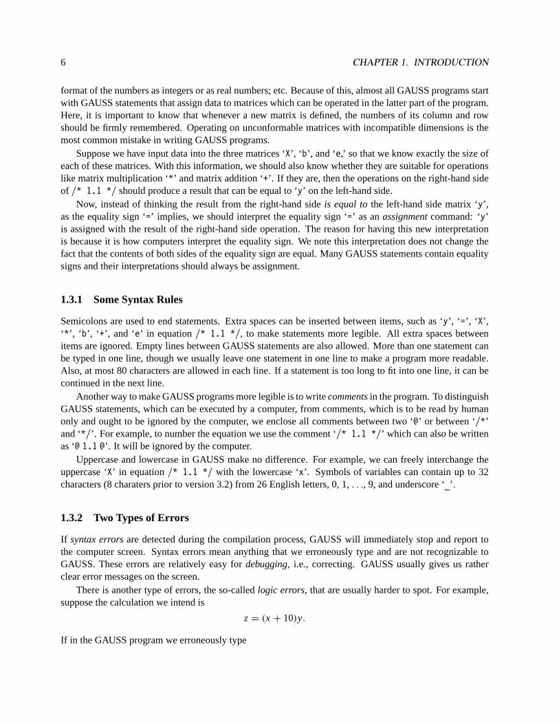
1.1.1 Executing DOS Commands in GAUSS
We can access all the DOS commands from the GAUSS command mode. In fact, other than running GAUSSprograms, what we do in the command mode are mostly DOS related activities such as copying or deletingfiles, making or changing directories, etc. To do these, we simply precede all the usual DOS commands with’dos’. For example, to copy the fileprg.1 to another fileprg.2, we type
1 dos copy prg.1 prg.2
There is a big advantage in executing DOS commands in the command mode: all the commands will stayon the screen so they can be revised or reused. You do not have to retype the entire command again andagain when the same command is to be repeated.
1.1.2 Some GAUSS Keystrokes
All the commands to be executed in the command mode need to be preceded by the GAUSS prompt ‘>>’. Ifthere is no GAUSS prompt on the screen, press theF3 key to create one. There are some other useful keysin the command mode:
• The four arrow keys: to move the cursor around the screen.
• The ‘Home’ keys: to go to the end of the line and then the end of the screen.

4 CHAPTER 1. INTRODUCTION
• The ‘Backspace’ key: to delete a character to the left.
• The ‘Del’ key: to delete a character.
• The ‘Escape’ key: to exit form the command mode and go back to DOS.
• F1: to recall the previous screen.
• Ctrl-F2: to execute the file that was last run.
• Ctrl-Enter (pressing the ‘Ctrl’ and ‘Enter’ keys simultaneously): to add a blank line.
• Ctrl-Home: to clear the screen.
• Ctrl-N: to add a blank line.
• Alt-D: to delete a line.
• Alt-H: to access the On-Line Help, which provides a fairly detailed description of all GAUSS com-mands. The use of On-Line Help is quite self-explanatory. After Alt-H is pressed, a help screen willbe displayed. Pressing ‘H’ again will give us the prompt ‘Help On:’ at the bottom of the screen. It isfrom this prompt we can access all other On-Line Help information. More about On-Line Help willbe discussed in sections 4.5 and 9.5.
1.1.3 A Note on Computer Memory
GAUSS can automatically access all the memory in the computer. 4MB memory is the minimum require-ment for GAUSS-386 version 3.2. Occasionally, the “insufficient memory” problem may occur. Other thanadding more memory chips to the computer, an easier remedy is use another version of GAUSS: GAUSS-386VM. The letters “VM” means it can transform the hard disk space toVirtual Memory- a kind of simulatedmemory. The disadvantage of using virtual memory is that computation slows down considerably.
1.2 The GAUSS Editor
This section presents a brief explanation of the GAUSS editor. It is a part of the GAUSS that is used totyped and revise the GAUSS program in an ASCII file. Although we may use a wordprocessor or someother editor like the DOS editor for such tasks, the advantage of using GAUSS editor is that the GAUSSprogram can be submitted for execution directly from inside the GAUSS editor. The commands describedhere are not complete but will get almost all your editing jobs done. To use the GAUSS editor to edit anASCII file, say,prg.0 in the command mode, we type
1 edit prg.0
and press the ‘Enter’ key after the GAUSS prompt ‘>>’ . The content of the file ‘prg.0’, if any, will appearon the screen ready for editing. All the keys for the command mode described in the previous section stillwork inside the GAUSS editor and there are many more. Let’s first consider an important feature of theGAUSS editor – blocking. Multi-line text in a file can beblockedfor special uses. To block off a section

1.3. GAUSS STATEMENTS 5
of text, press Alt-L at both ends. The blocked text will then be highlighted. The blocked text can be copiedor moved to other places in the file. To do this, either press the ‘+’ key in the numeric keypad tocopytheblocked text to scrap (which is a temporary storage place outside the file), or press the ‘-’ key in the numerickeypad tomovethe blocked text to scrap. After the scrap is filled with some data, then move the cursorto another place and press the ‘Ins’ key to retrieve the blocked text from the scrap. As such the blockedtext can be copied or moved to any place in the file. The blocked text can be further manipulated by thefollowing keystrokes:
• Alt-W: to copy the blocked text to another file.
• Ctrl-X: to execute the blocked text.
• Alt-P: to print the blocked text.
• The ‘Del’ key: to delete the blocked text.
Text can be searched and replaced using the GAUSS editor:
• F5: for searching.
• F6: for searching and replacing.
After we finish editing, there are three ways to exit the GAUSS editor and go back to the command mode:
• Alt-X: a menu of options will show up for selection.
• F1: to save the file and exit.
• F2: to save the file and then execute it.
While in the command mode after editing a file, there are several keys related to the GAUSS editor:
• Shift-F1: to directly go back to the last edited file for additional editing.
• Shift-F2: to execute the last edited file again automatically.
• Ctrl-F1: to edit the last run file automatically, given that a file has just been run.
• Ctrl-F3: to edit the last output file automatically, given that a file has just been run which produces anoutput file.
These keystrokes may be difficult to remember at first. But just a few exercises can change such feelingcompletely.
1.3 GAUSS Statements
Equation/* 1.1 */ in page 1 is a typical GAUSS statement which contains an equality sign. It is theGAUSS counterpart of the handwritten equation (1.1). When we write down an equation like (1.1) onscratch paper, the exact values ofy, X, βββ, andεεε do not really concern us. However, when we type equation/* 1.1 */ in a GAUSS program, we need to be very specific about the values in the matrices ‘y’, ‘ X’, ‘ b’,and ‘e’ as to what exactly are contained in each matrix: how many variables, how many observations, the
6 CHAPTER 1. INTRODUCTION
format of the numbers as integers or as real numbers; etc. Because of this, almost all GAUSS programs startwith GAUSS statements that assign data to matrices which can be operated in the latter part of the program.Here, it is important to know that whenever a new matrix is defined, the numbers of its column and rowshould be firmly remembered. Operating on unconformable matrices with incompatible dimensions is themost common mistake in writing GAUSS programs.
Suppose we have input data into the three matrices ‘X’, ‘ b’, and ‘e,’ so that we know exactly the size ofeach of these matrices. With this information, we should also know whether they are suitable for operationslike matrix multiplication ‘*’ and matrix addition ‘+’. If they are, then the operations on the right-hand sideof /* 1.1 */ should produce a result that can be equal to ‘y’ on the left-hand side.
Now, instead of thinking the result from the right-hand sideis equal tothe left-hand side matrix ‘y’,as the equality sign ‘=’ implies, we should interpret the equality sign ‘=’ as anassignmentcommand: ‘y’is assigned with the result of the right-hand side operation. The reason for having this new interpretationis because it is how computers interpret the equality sign. We note this interpretation does not change thefact that the contents of both sides of the equality sign are equal. Many GAUSS statements contain equalitysigns and their interpretations should always be assignment.
1.3.1 Some Syntax Rules
Semicolons are used to end statements. Extra spaces can be inserted between items, such as ‘y’, ‘ =’, ‘ X’,‘*’, ‘ b’, ‘ +’, and ‘e’ in equation/* 1.1 */, to make statements more legible. All extra spaces betweenitems are ignored. Empty lines between GAUSS statements are also allowed. More than one statement canbe typed in one line, though we usually leave one statement in one line to make a program more readable.Also, at most 80 characters are allowed in each line. If a statement is too long to fit into one line, it can becontinued in the next line.
Another way to make GAUSS programs more legible is to writecommentsin the program. To distinguishGAUSS statements, which can be executed by a computer, from comments, which is to be read by humanonly and ought to be ignored by the computer, we enclose all comments between two ‘@’ or between ‘/*’and ‘*/’. For example, to number the equation we use the comment ‘/* 1.1 */’ which can also be writtenas ‘@ 1.1 @’. It will be ignored by the computer.
Uppercase and lowercase in GAUSS make no difference. For example, we can freely interchange theuppercase ‘X’ in equation/* 1.1 */ with the lowercase ‘x’. Symbols of variables can contain up to 32characters (8 charaters prior to version 3.2) from 26 English letters, 0, 1,. . ., 9, and underscore ‘_’.
1.3.2 Two Types of Errors
If syntax errorsare detected during the compilation process, GAUSS will immediately stop and report tothe computer screen. Syntax errors mean anything that we erroneously type and are not recognizable toGAUSS. These errors are relatively easy fordebugging, i.e., correcting. GAUSS usually gives us ratherclear error messages on the screen.
There is another type of errors, the so-calledlogic errors, that are usually harder to spot. For example,suppose the calculation we intend is
z = (x + 10)y.
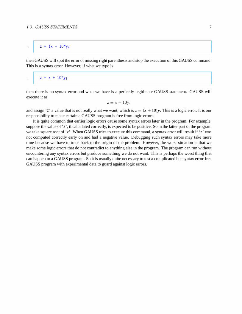
If in the GAUSS program we erroneously type
1.3. GAUSS STATEMENTS 7
1 z = (x + 10*y;
then GAUSS will spot the error of missing right parenthesis and stop the execution of this GAUSS command.This is a syntax error. However, if what we type is
1 z = x + 10*y;
then there is no syntax error and what we have is a perfectly legitimate GAUSS statement. GAUSS willexecute it as
z = x + 10y,
and assign ‘z’ a value that is not really what we want, which isz = (x + 10)y. This is a logic error. It is ourresponsibility to make certain a GAUSS program is free from logic errors.
It is quite common that earlier logic errors cause some syntax errors later in the program. For example,suppose the value of ‘z’, if calculated correctly, is expected to be positive. So in the latter part of the programwe take square root of ‘z’. When GAUSS tries to execute this command, a syntax error will result if ‘z’ wasnot computed correctly early on and had a negative value. Debugging such syntax errors may take moretime because we have to trace back to the origin of the problem. However, the worst situation is that wemake some logic errors that do not contradict to anything else in the program. The program can run withoutencountering any syntax errors but produce something we do not want. This is perhaps the worst thing thatcan happen to a GAUSS program. So it is usually quite necessary to test a complicated but syntax error-freeGAUSS program with experimental data to guard against logic errors.

8 CHAPTER 1. INTRODUCTION

Chapter 2Data Input and Output
Consider the definition of the error term in equation (1.1):
εεε = y − Xβββ. (2.1)
Suppose we have data on the dependent variabley and a few explanatory variablesX. The parameter vectorβββ is also known to us. If we want to compute the error vectorεεε, then we use the GAUSS command
1 e = y - X*b; /* 2.1 */
Let’s assume the data consist ofN observations and there areK explanatory variables. So the dimensionsof the matricesy, X, andβββ aren × 1, n × k, andk × 1, respectively. Suppose these data are recorded ona piece of paper, then the question is: how can we read these data into the matrices ‘y’, ‘ X’, and ‘b’ in aGAUSS program?
2.1 ASCII Files
The most straightforward way to read data into matrices is through the direct assignment statements asfollows:
1 y = {1, 3, 4.5, -4, 5};2
3 X = {1 4.2 6.1,4 1 3.9 2.7,5 1 2.4 0,6 1 -7.35 3.2,7 1 6.8 2.2};8
9 b = {2.1, 0.3, 2.2};
The numbers on the right-hand side are our hypothetical data. Note that we haven = 5 andk = 3 here. (Asmentioned earlier, keeping these dimensions in mind is important in writing GAUSS programs.) From thepattern the data is listed, it is easy to infer that commas separate rows, spaces separate columns, and all dataare enclosed in braces.
There is no difference between the second assignment statement for ‘X’ and the following one:
1 X = {1 4.2 6.1, 1 3.9 2.7, 1 2.4 0, 1 -7.35 3.2, 1 6.8 2.2};
9
10 CHAPTER 2. DATA INPUT AND OUTPUT
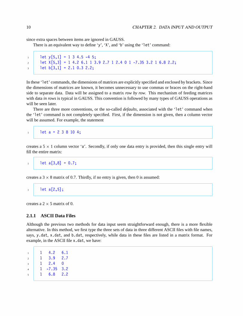
since extra spaces between items are ignored in GAUSS.There is an equivalent way to define ‘y’, ‘ X’, and ‘b’ using the ‘let’ command:
1 let y[5,1] = 1 3 4.5 -4 5;2 let X[5,3] = 1 4.2 6.1 1 3.9 2.7 1 2.4 0 1 -7.35 3.2 1 6.8 2.2;3 let b[3,1] = 2.1 0.3 2.2;
In these ‘let’ commands, the dimensions of matrices are explicitly specified and enclosed by brackets. Sincethe dimensions of matrices are known, it becomes unnecessary to use commas or braces on the right-handside to separate data. Data will be assigned to a matrixrow by row. This mechanism of feeding matriceswith datain rows is typical in GAUSS. This convention is followed by many types of GAUSS operations aswill be seen later.
There are three more conventions, or the so-calleddefaults, associated with the ‘let’ command whenthe ‘let’ command is not completely specified. First, if the dimension is not given, then a column vectorwill be assumed. For example, the statement
1 let a = 2 3 8 10 4;
creates a 5× 1 column vector ‘a’. Secondly, if only one data entry is provided, then this single entry willfill the entire matrix:
1 let a[3,8] = 0.7;
creates a 3× 8 matrix of 0.7. Thirdly, if no entry is given, then 0 is assumed:
1 let a[2,5];
creates a 2× 5 matrix of 0.
2.1.1 ASCII Data Files
Although the previous two methods for data input seem straightforward enough, there is a more flexiblealternative. In this method, we first type the three sets of data in three different ASCII files with file names,says,y.dat, x.dat, andb.dat, respectively, while data in these files are listed in a matrix format. Forexample, in the ASCII filex.dat, we have:
1 1 4.2 6.12 1 3.9 2.73 1 2.4 04 1 -7.35 3.25 1 6.8 2.2

2.1. ASCII FILES 11
Note that no commas or braces are included. Given the three ASCII data files, we use the following threeGAUSS commands to read data from them:
1 load y[5,1] = y.dat;2 load X[5,3] = x.dat;3 load b[3,1] = b.dat;
Again, the dimensions of matrices need to be explicitly specified in these ‘load’ commands. This data inputmethod is the most common one because we do not always type data ourselves but obtain some ASCII datafiles from somewhere else.
In most ASCII data files, data are displayed just like those in the abovex.dat example: different vari-ables are listed in columns, which are separated by spaces, and observations are listed along rows. However,as mentioned earlier, GAUSS has the automatic mechanism of feeding matrices in rows. So the data in theASCII file x.dat can actually be listed as
1 1 4.2 6.1 1 3.9 2.7 1 2.4 02 1 -7.35 3.2 1 6.8 2.2
As long as the dimension of ‘x’ in the ‘load’ command is correctly specified, data will be loaded into ‘x’correctly – one row by another.
2.1.2 ASCII Output Files
After data have been read into the matrices ‘y’, ‘ X’, and ‘b’, the assignment operation /* 2.1 */ can then beexecuted to create the error vector ‘e’. The question now is how we can access the resulting values in ‘e’,either to read them or to store them for later uses. Consider the following GAUSS statements:
1 output file = residual.out on;2 format /rd 10,4;3 print e;
The ‘output file’ command in the first lineopens(i.e., creates or retrieves) an ASCII file with the name‘residual.out’, which can be any file name with extension that follows the standard rule for file names.The file ‘residual.out’ can be a new file or an existing file. If ‘residual.out’ is an existing file withsome data already in it, then the subcommand ‘on’ causes new data, which we are about to produce, tobe appended onto the end of this file without affecting those existing data. An alternative subcommand is‘reset’ which resets the referred file so that all the existing data will be erased.
The ‘format’ command in the second line describes how the data should be listed in the output file. Itssecond subcommand ‘/rd’ means the listed data are to be right-justified and the third subcommand ‘10,4’means in total ten spaces are reserved for each entry which is rounded to four digits after the decimal point.The ‘10,4’ subcommand may be changed to suit different needs. A common one is ‘6,0’ which means tolist the values as integer numbers (without decimal points) over six spaces.
Although there are seven other alternatives, the ‘/rd’ subcommand is used most often. Another commonone is ‘/re’, with which the value 0.012345(= 1.2345× 10⁻²) will be listed as 1.2345E-2 (given the other

12 CHAPTER 2. DATA INPUT AND OUTPUT
subcommand is ‘6,4’). If left-justified listing is desired, change ‘r’ in the above subcommands to ‘l’.To find out more about the other possibilities, press Alt-H and then type ‘format’. On-Line Help for the‘format’ command will appear. (There we can find a third subcommand which is much less used.)
The ‘print’ command in the third line means to list all the elements of ‘e’. The results will be listedboth on the computer screen as well as in the output ASCII fileresidual.out using the format specified bythe ‘format’ command. The ‘print’ command can be abbreviated as
1 e;
That is, we simply type the name of the matrix, followed by a semicolon. This simplified print commandwill be used throughout this book.
A GAUSS program can contain more than one print command. All the printed matrices will be includedin the same output ASCII file and follow the format based on the ‘format’ command that is last executed.
Once the output ASCII file is created with data printed into it, we can use a word processor or an editorto view, revise, or print those data.
The data in the output ASCII file, like any ASCII data file, can also be read back into a matrix in aGAUSS program using the ‘load’ command as described earlier. For example, the entries listed in theASCII file residual.out can be loaded back to the matrix ‘e’ as follows:
1 load e[5,1] = residual.out;
Note that when an ASCII data file is loaded, we have to make sure the number of data entries in the ASCIIfile matches the matrix size specified in the ‘load’ command. Again, no matter how the data entries arelisted in the ASCII file, they will be read into the matrix row by row.
2.1.3 Other Commands Related to ASCII Output Files
Suppose we do not want the values in ‘e’ to be listed in any ASCII file and all we want is to read them onthe screen, then we just skip the ‘output file’ command.
If an output ASCII file is already opened, it can be ‘closed’ by
1 output off;
The output file can be reopened again to accept new output entries by
1 output on;
If we want to list results from several operations at several places in a long program, we can open an ASCIIfile at the beginning of the program and then close and reopen it as often as we want.
If an empty line is to be included in the output file between two printed matrices, then between the two‘print’ commands type:
1 print;
2.1. ASCII FILES 13
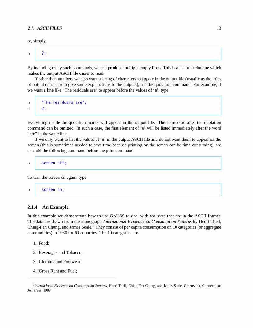
or, simply,
1 ?;
By including many such commands, we can produce multiple empty lines. This is a useful technique whichmakes the output ASCII file easier to read.
If other than numbers we also want a string of characters to appear in the output file (usually as the titlesof output entries or to give some explanations to the outputs), use the quotation command. For example, ifwe want a line like “The residuals are” to appear before the values of ‘e’, type
1 "The residuals are";2 e;
Everything inside the quotation marks will appear in the output file. The semicolon after the quotationcommand can be omitted. In such a case, the first element of ‘e’ will be listed immediately after the word“are” in the same line.
If we only want to list the values of ‘e’ in the output ASCII file and do not want them to appear on thescreen (this is sometimes needed to save time because printing on the screen can be time-consuming), wecan add the following command before the print command:
1 screen off;
To turn the screen on again, type
1 screen on;
2.1.4 An Example
In this example we demonstrate how to use GAUSS to deal with real data that are in the ASCII format.The data are drawn from the monographInternational Evidence on Consumption Patterns by Henri Theil,Ching-Fan Chung, and James Seale.1 They consist of per capita consumption on 10 categories (or aggregatecommodities) in 1980 for 60 countries. The 10 categories are
1. Food;
2. Beverages and Tobacco;
3. Clothing and Footwear;
4. Gross Rent and Fuel;
1International Evidence on Consumption Patterns, Henri Theil, Ching-Fan Chung, and James Seale, Greenwich, Connecticut:JAI Press, 1989.

14 CHAPTER 2. DATA INPUT AND OUTPUT
5. House Furnishings and Operations;
6. Medical Care;
7. Transport and Communications;
8. Recreation;
9. Education; and
10. Other.
The data are in three ASCII files whose names are ‘volume’, ‘ share’, and ‘totalexp’, respectively.Both ‘volume’ and ‘share’ files contain 60× 10 matrices. The 60 rows correspond to the observations onthe 60 countries and 10 columns for 10 categories.
The data in the file ‘volume’ are the volumes of per capita consumption (in terms of a set of stan-dardized measurement units). These volumes can be considered as thequantities qic, i = 1, . . . ,10 andc = 1, . . . ,60, of the 10 commodities.
If in addition to these quantities, we also haveprices pic, then we can define theexpenditureson these10 commodities simply by the productspicqic, from which we can also define thetotal expenditures:
mc =
10∑i =1
picqic, c = 1, . . . ,60.
The file ‘totalexp’ is a 60× 1 vector which contains the data on the 60 countries’ total expendituremc.Note that a country’s total expendituremc can also be referred to as it’s income.
Finally, we note thebudget sharesof the commodities are defined by
sic =picqic
mc, i = 1, . . . ,10, c = 1, . . . ,60.
The file ‘share’ contains the 60 observations on 10 budget shares.Suppose we want to read data from these three different ASCII files and then print them in a single ASCII
file calledall.out with some description. We use the editor to type the following GAUSS commands in anASCII file, say,try.1:
1 load q[60,10] = a:\data\volume;2 load s[60,10] = a:\data\share;3 load m[60,1] = a:\data\totalexp;4
5 output file = a:\all.out on;6
7 "The Quantities of 10 Commodities from 60 Countries:";?;8 format /rd 8,2;9 q;?;?;?;
10
11 "The Budget Shares of 10 Commodities from 60 Countries:";?;12 s;?;?;?;
2.2. MATRIX FILES 15
13
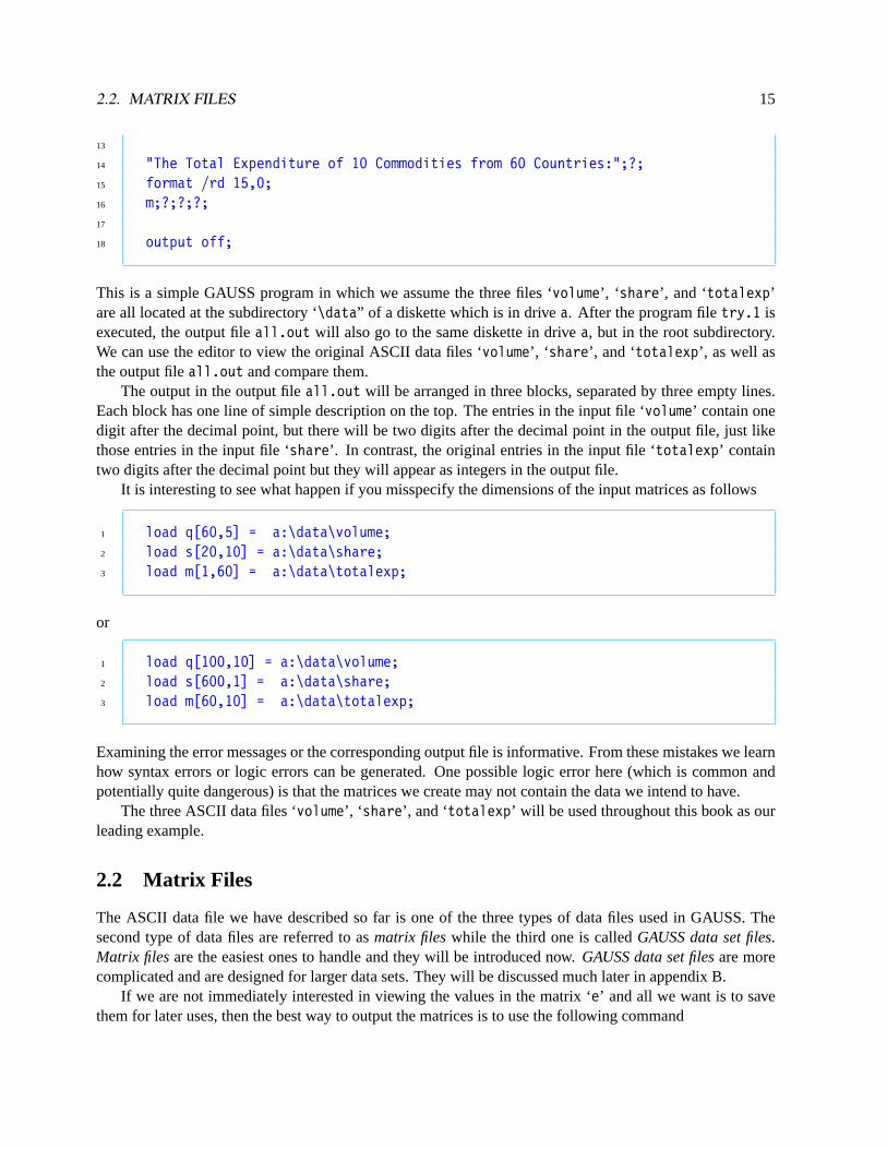
14 "The Total Expenditure of 10 Commodities from 60 Countries:";?;15 format /rd 15,0;16 m;?;?;?;17
18 output off;
This is a simple GAUSS program in which we assume the three files ‘volume’, ‘ share’, and ‘totalexp’are all located at the subdirectory ‘\data” of a diskette which is in drivea. After the program filetry.1 isexecuted, the output fileall.out will also go to the same diskette in drivea, but in the root subdirectory.We can use the editor to view the original ASCII data files ‘volume’, ‘ share’, and ‘totalexp’, as well asthe output fileall.out and compare them.
The output in the output fileall.out will be arranged in three blocks, separated by three empty lines.Each block has one line of simple description on the top. The entries in the input file ‘volume’ contain onedigit after the decimal point, but there will be two digits after the decimal point in the output file, just likethose entries in the input file ‘share’. In contrast, the original entries in the input file ‘totalexp’ containtwo digits after the decimal point but they will appear as integers in the output file.
It is interesting to see what happen if you misspecify the dimensions of the input matrices as follows
1 load q[60,5] = a:\data\volume;2 load s[20,10] = a:\data\share;3 load m[1,60] = a:\data\totalexp;
or
1 load q[100,10] = a:\data\volume;2 load s[600,1] = a:\data\share;3 load m[60,10] = a:\data\totalexp;
Examining the error messages or the corresponding output file is informative. From these mistakes we learnhow syntax errors or logic errors can be generated. One possible logic error here (which is common andpotentially quite dangerous) is that the matrices we create may not contain the data we intend to have.
The three ASCII data files ‘volume’, ‘ share’, and ‘totalexp’ will be used throughout this book as ourleading example.
2.2 Matrix Files
The ASCII data file we have described so far is one of the three types of data files used in GAUSS. Thesecond type of data files are referred to asmatrix fileswhile the third one is calledGAUSS data set files.Matrix filesare the easiest ones to handle and they will be introduced now.GAUSS data set filesare morecomplicated and are designed for larger data sets. They will be discussed much later in appendix B.
If we are not immediately interested in viewing the values in the matrix ‘e’ and all we want is to savethem for later uses, then the best way to output the matrices is to use the following command

16 CHAPTER 2. DATA INPUT AND OUTPUT
1 save e;
The data in ‘e’ will be saved as amatrix file with the file name ‘e.fmt’, where the extension ‘.fmt’ isautomatically attached to the matrix name. In the GAUSS program we do not need to specify the format ordimension for matrix files. Data will be automatically stored with the maximum precision.
The disadvantage of storing data in matrix files is that they cannot be viewed with a word processor oran editor. To find out what are inside a matrix file, we have to first load the matrix file back to a matrix in aGAUSS program and then print it on the screen or in an ASCII file. However, to load a matrix file is quiteeasy. For example, to load thee.fmt file back, just type
1 load e;
It is possible to change the name of the matrix file when it is saved. For example, the command
1 save res = e;
will save data in the matrix file ‘res.fmt’. The extension ‘.fmt’ is again automatically attached. So whenwe specify the file name in the ‘save’ command, no extension should be included. If the fileres.fmt is tobe loaded back to a matrix with the name ‘a’, type
1 load a = res;
Since it is not necessary to type the extension ‘.fmt’ or to specify the dimension of the matrix ‘a’, it is easierthan loading an ASCII data file.
Consider the following simple example:
1 load q[60,10] = a:\data\volume;2 load s[60,10] = a:\data\share;3 load m[60,1] = a:\data\totalexp;4
5 save a:\data\volume = q,6 a:\data\share = s,7 a:\data\totalexp = m;
After these commands being executed, the directorya:\data\share will then contain three more files:volume.fmt, share.fmt, andtotalexp.fmt. They are matrix files. They are different from the three orig-inal ASCII data files ‘volume’, ‘ share’, and ‘totalexp’, which do not have the ‘.fmt’ extension (althoughthe contents are the same).
Chapter 3Basic Algebraic Operations
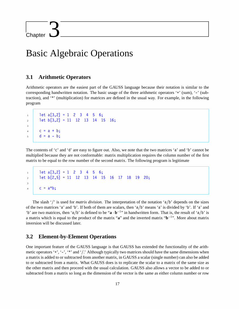
3.1 Arithmetic Operators
Arithmetic operators are the easiest part of the GAUSS language because their notation is similar to thecorresponding handwritten notation. The basic usage of the three arithmetic operators ‘+’ (sum), ‘-’ (sub-traction), and ‘*’ (multiplication) for matrices are defined in the usual way. For example, in the followingprogram
1 let a[3,2] = 1 2 3 4 5 6;2 let b[3,2] = 11 12 13 14 15 16;3
4 c = a + b;5 d = a - b;
The contents of ‘c’ and ‘d’ are easy to figure out. Also, we note that the two matrices ‘a’ and ‘b’ cannot bemultiplied because they are not conformable: matrix multiplication requires the column number of the firstmatrix to be equal to the row number of the second matrix. The following program is legitimate
1 let a[3,2] = 1 2 3 4 5 6;2 let b[2,5] = 11 12 13 14 15 16 17 18 19 20;3
4 c = a*b;
The slash ‘/’ is used formatrix division. The interpretation of the notation ‘a/b’ depends on the sizesof the two matrices ‘a’ and ‘b’. If both of them are scalars, then ‘a/b’ means ‘a’ is divided by ‘b’. If ‘ a’ and‘b’ are two matrices, then ‘a/b’ is defined to be “a · b−1” in handwritten form. That is, the result of ‘a/b’ isa matrix which is equal to the product of the matrix “a” and the inverted matrix “b−1”. More about matrixinversion will be discussed later.
3.2 Element-by-Element Operations
One important feature of the GAUSS language is that GAUSS has extended the functionality of the arith-metic operators ‘+’, ‘ -’, ‘ *’ and ‘/.’ Although typically two matrices should have the same dimensions whena matrix is added to or subtracted from another matrix, in GAUSS a scalar (single number) can also be addedto or subtracted from a matrix. What GAUSS does is to replicate the scalar to a matrix of the same size asthe other matrix and then proceed with the usual calculation. GAUSS also allows a vector to be added to orsubtracted from a matrix so long as the dimension of the vector is the same as either column number or row
17
18 CHAPTER 3. BASIC ALGEBRAIC OPERATIONS
number of the other matrix. What GAUSS does again is to replicate the vector to a conformable matrix. Forexample, suppose ‘a’ is a 1× 4 row vector and ‘b’ is a 6× 4 matrix. When computing ‘a + b’, GAUSSfirst replicates ‘a’ six times to form a 6× 4 matrix with six identical rows and then adds this matrix to ‘b’.
There are two new operators ‘.*’ and ‘./’ (i.e., ‘*’ and ‘/’ preceded by a dot) in GAUSS that arereferred to as element-by-element multiplication and element-by-element division, respectively. Given that‘a’ and ‘b’ are two matrices of the same dimensions, ‘a.*b’ means that each element of ‘a’ is multiplied bythe corresponding element in ‘b’ and ‘a./b’ means that each element of ‘a’ is divided by the correspondingelement in ‘b.’
Since the rule of element-by-element multiplication and element-by-element division about the dimen-sion work is the same as matrix addition, it is also possible for the two matrices under the element-by-element operation to have different dimensions: GAUSS simply expands the matrix of the smaller sizebefore operates on it.
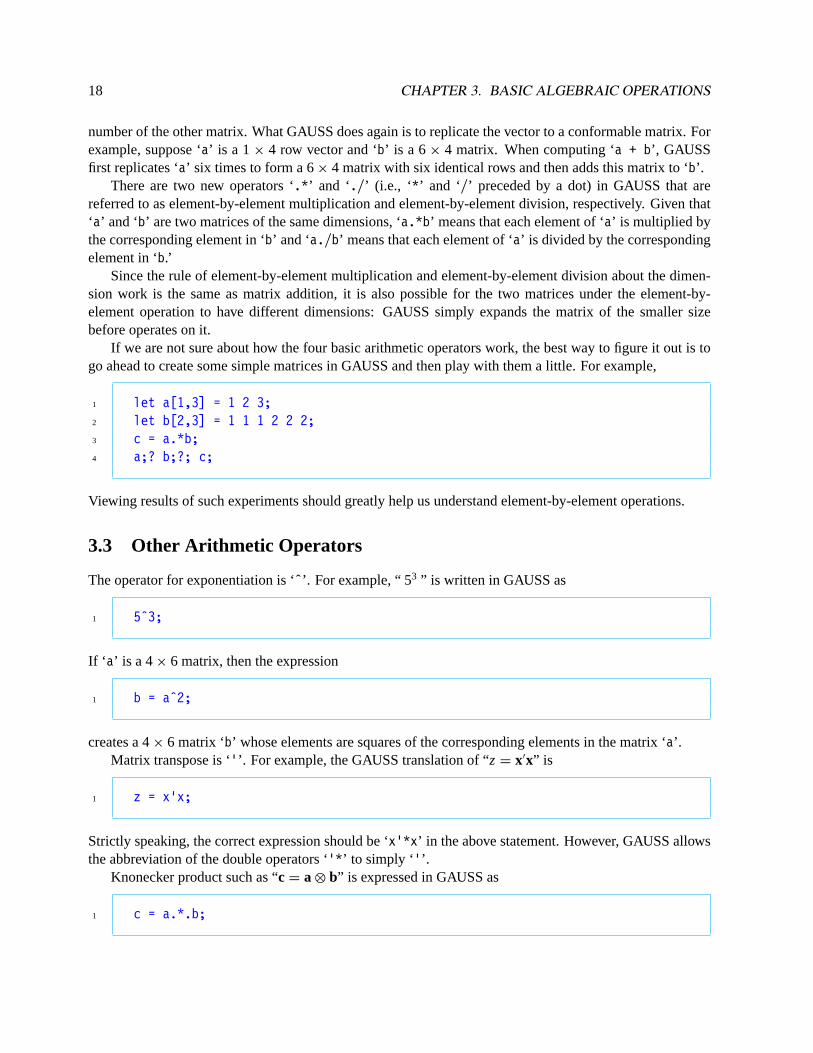
If we are not sure about how the four basic arithmetic operators work, the best way to figure it out is togo ahead to create some simple matrices in GAUSS and then play with them a little. For example,
1 let a[1,3] = 1 2 3;2 let b[2,3] = 1 1 1 2 2 2;3 c = a.*b;4 a;? b;?; c;
Viewing results of such experiments should greatly help us understand element-by-element operations.
3.3 Other Arithmetic Operators
The operator for exponentiation is ‘ˆ’. For example, “ 53 ” is written in GAUSS as
1 5ˆ3;
If ‘ a’ is a 4× 6 matrix, then the expression
1 b = aˆ2;
creates a 4× 6 matrix ‘b’ whose elements are squares of the corresponding elements in the matrix ‘a’.Matrix transpose is ‘’’. For example, the GAUSS translation of “z = x′x” is
1 z = x’x;
Strictly speaking, the correct expression should be ‘x’*x’ in the above statement. However, GAUSS allowsthe abbreviation of the double operators ‘’*’ to simply ‘’’.
Knonecker product such as “c = a ⊗ b” is expressed in GAUSS as
1 c = a.*.b;

3.4. PRIORITY OF THE ARITHMETIC OPERATORS 19
If the dimensions of the matrices ‘a’ and ‘b’ are m × n and p × q, respectively, then the resulting ‘c’ is ablocked matrix containingm × n blocks. The(i, j )-th block is a matrix of the dimensionp × q which isthe product of the(i, j )-th element in the matrix ‘a’ and the entire matrix ‘b’. So the dimension of ‘c’ ismp× nq.
3.4 Priority of the Arithmetic Operators
If more than one operator appear in the same expression, some operators will be performed prior to theothers. For example, matrix multiplication has higher priority than matrix addition: 2+ 3 · 4 is equal to2 + (3 · 4) instead of(2 + 3) · 4. Also, [(a + b)c]2 is different froma + b · c2 because the priority ofexponentiation operation is higher than both multiplication and addition. Here, we note that parentheses andbrackets help to rearrange the priority of the operations. Generally speaking, the usual priority rule we learnfrom high school algebra still applies to the GAUSS operation and it is not necessary to memorize any newrule.
Note that the GAUSS expression for computing [(a + b)c]2 is ‘((a + b)*c)ˆ2’. Since the brackets arenot used in GAUSS, we need two layers of parentheses here in the GAUSS expression. The best way toavoid trouble when we are not sure about the priority of some operators is to use parentheses generously.
An Example Given data on quantitiesqic, budget sharessic, and incomemc of 10 commodities in theASCII files ‘volume’, ‘ share’, and ‘totalexp’, we can compute the expenditureseic and pricespic, where
eic ≡ picqic = mcpicqic
mc≡ mcsic,
from which we can also compute the prices
pic =picqic
qic≡
eic
qic.
In the following GAUSS program we load the ASCII data files, compute the 10 expenditures and prices for60 countries, and then print the results in an output file named ‘comp.out’:
1 load q[60,10] = a:\data\volume;2 load s[60,10] = a:\data\share;3 load m[60,1] = a:\data\totalexp;4
5 e = m.*s;6 p = e./q;7
8 output file = comp.out reset;9 format /rd 8,2;
10
11 "The Expenditures of 10 Commodities:";?;12 e;?;?;13
14 "The Prices of 10 Commodities:";?;

20 CHAPTER 3. BASIC ALGEBRAIC OPERATIONS
15 p;?;?;16
17 output off;18
19 save q, p, m;
The output ASCII filecomp.out from this simple program will contain two 60× 10 matrices: the expen-ditures and the prices of the 10 commodities from 60 countries. The quantities, prices, and income arealso stored as matrix files with nameq.fmt, p.fmt, andm.fmt, respectively. Because we do not explicitlyspecify the subdirectory and drive names, all output files are located at the current subdirectory in drivec(which is the default).
Note that the 60× 10 matrices ‘e’ and ‘p’ of expenditures and prices are computed using the element-by-element multiplication and element-by-element division, respectively. In particular, we note that ‘m’ isonly a 60× 1 column vector while ‘s’ is a 60× 10 matrix. When they are multiplied, GAUSS first expands‘m’ to a 60× 10 matrix with identical columns and then multiplies it, element by element, to the matrix ‘s’.These examples show how convenient the element-by-element operations are.
3.5 Matrix Concatenation and Indexing Matrices
One of the most useful features of GAUSS is it allows us to manipulate matrices almost anyway we want.We can combine several matrices byconcatenationor extract part of a matrix byindexing.
If ‘ a’ is a 3× 4 matrix and ‘b’ is a 3× 2 matrix, then they can be concatenated horizontally to a 3× 6matrix as follows:
1 c = a˜b;
The first four columns of ‘c’ come from ‘a’ and the last two columns come from ‘b’. Similarly, two matrices‘d’ and ‘e’ with the same column numbers can be concatenated vertically as follows:
1 f = d|e;
If we want to extract the second and fourth rows of a matrix ‘a’ to form a new matrix ‘b’ of two rows,then we type
1 b = a[2 4,.];
The two numbers in the brackets before the comma are row indices and the numbers, if any, after the commaare column indices. In the above case, the column indices are replaced by a dot ‘.’ which means all columnsare selected. If we want to extract the third and fourth columns of a matrix ‘a’ to form a new matrix ‘b’ oftwo columns, then we type
1 b = a[.,3 4];

3.5. MATRIX CONCATENATION AND INDEXING MATRICES 21
If we want to extract the first, fourth and second rows, and the fifth column of a matrix ‘a’ to form a 3× 1matrix ‘b’, then we type
1 b = a[1 4 2,5];
Note that the indices can be in any order so that we can rearrange the elements of a matrix in any order wewant.
Let’s consider the problem of reading data to the matrices ‘y’ and ‘X’ of the equation/* 2.1 */. Sup-pose the data ‘y’ and ‘X’ are stored together in a 5× 4 matrix format in the ASCII file ‘all.dat’, wherethe first column of the matrix contains the data for ‘y’ and the last three columns are for ‘X’. We use thefollowing statements to read the data into ‘y’ and ‘X’:
1 load alldata[5,4] = all.dat;2
3 y = alldata[.,1];4 X = alldata[.,2:4];
When defining ‘X’, we use ‘2:4’ to denote the column indices ‘2 3 4’. The colon mark can be used toabbreviate consecutive indices.
An Example Suppose we are interested in the International Consumption data on Food and we want tolist quantities, prices, and budget shares, together with income in one ASCII filefood.out. Here we canuse the three matrix filesq.fmt, p.fmt, andy.fmt created earlier as the inputs.
1 load food_q = q, food_p = p, y;2
3 food_q = food_q[.,1];4 food_p = food_p[.,1];5 food_s = (food_q.*food_p)./y;6
7 out = food_q˜food_p˜food_s˜y;8
9 output file = food.out reset;10 format /rd 10,2;11
12 out;13
14 output off;
Note that when we load the matrix files ‘q’ and ‘p’, we change their names to ‘food_q’ and ‘food_p’,respectively. Since Food data are in the first column of these matrices, the matrix indexing technique isapplied to pick these columns. We also note that the resulting column vectors for Food data are againnamed as ‘food_q’ and ‘food_q’, respectively. Such reuse of the matrix names in assignment commands

22 CHAPTER 3. BASIC ALGEBRAIC OPERATIONS
is perfectly acceptable. However, we should know that after the execution of these commands, the original60× 10 matrices ‘food_q’ and ‘food_q’ will no longer exist (in the computer memory) because they havebeen completely replaced by 60× 1 column vectors of the Food data. The main reason for adopting sucha trick is to economize the number of matrices. Since each matrix occupies some computer memory, it isalways desirable to get rid of those matrices which are no longer needed to release the computer memoryfor other uses.
Another way to clear unwanted matrices is to directly set them to zero. For example, immediately afterthe ‘out’ matrix is defined we can have the following expressions:
1 food_q = 0;2 food_p = 0;3 food_s = 0;4 y = 0;
Here are a few interesting questions about the above program:
• What is the size of the matrix ‘out’?
• What is the format of the print-out in the output file ‘food.out’?
• How can we modify the above program so that the output contains data for the first ten and the lastten countries only?
The answer: first change ‘food_q[.,1]’ and ‘food_p[.,1]’ in the second and the third expressionsto ‘food_q[1:15 46:60,1]’ and ‘food_p[1:15 46:60,1]’, respectively, and then change ‘y’ in thefourth and fifth expressions to ‘y[1:15 46:60]’. Note that, since ‘y’ is a column, its second indexcan be omitted inside the brackets.
• How can we modify the above program to print out the results for a combined commodity of Foodand Beverages and Tobacco?
The answer: simply change ‘food_q[.,1]’ and ‘food_p[.,1]’ in the second and the third expres-sions to ‘food_q[.,1] + food_q[.,2]’ and ‘food_p[.,1] + food_p[.,2]’, respectively.
• Is it possible to print the matrix ‘out’ in a way that different columns have different formats?
The answer is no. To do this we need a special GAUSS command which will be discussed later.
Chapter 4GAUSS Commands
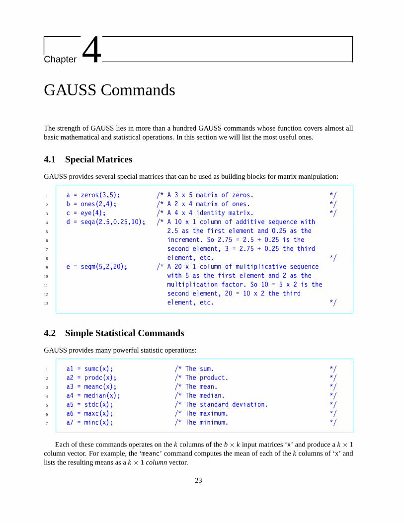
The strength of GAUSS lies in more than a hundred GAUSS commands whose function covers almost allbasic mathematical and statistical operations. In this section we will list the most useful ones.
4.1 Special Matrices
GAUSS provides several special matrices that can be used as building blocks for matrix manipulation:
1 a = zeros(3,5); /* A 3 x 5 matrix of zeros. */2 b = ones(2,4); /* A 2 x 4 matrix of ones. */3 c = eye(4); /* A 4 x 4 identity matrix. */4 d = seqa(2.5,0.25,10); /* A 10 x 1 column of additive sequence with5 2.5 as the first element and 0.25 as the6 increment. So 2.75 = 2.5 + 0.25 is the7 second element, 3 = 2.75 + 0.25 the third8 element, etc. */9 e = seqm(5,2,20); /* A 20 x 1 column of multiplicative sequence
10 with 5 as the first element and 2 as the11 multiplication factor. So 10 = 5 x 2 is the12 second element, 20 = 10 x 2 the third13 element, etc. */
4.2 Simple Statistical Commands
GAUSS provides many powerful statistic operations:
1 a1 = sumc(x); /* The sum. */2 a2 = prodc(x); /* The product. */3 a3 = meanc(x); /* The mean. */4 a4 = median(x); /* The median. */5 a5 = stdc(x); /* The standard deviation. */6 a6 = maxc(x); /* The maximum. */7 a7 = minc(x); /* The minimum. */
Each of these commands operates on thek columns of theb × k input matrices ‘x’ and produce ak × 1column vector. For example, the ‘meanc’ command computes the mean of each of thek columns of ‘x’ andlists the resulting means as ak × 1 columnvector.
23

24 CHAPTER 4. GAUSS COMMANDS
4.3 Simple Mathematical Commands
common mathematical operations are also easy to performed in GAUSS:
1 b1 = exp(x); /* The exponential function. */2 b2 = ln(x); /* The logarithmic function with the natural base. */3 b3 = log(x); /* The logarithmic function with base 10. */4 b4 = sqrt(x); /* The square root. */5 b5 = abs(x); /* The absolute value. */6
7 b6 = pi; /* The pi value 3.14159... */8 b7 = gamma(x); /* The gamma function. */9
10 b8 = sin(x); /* The sine function of x which is in radians. */11 b9 = cos(x); /* The cosine function of x which is in radians. */12 b10 = tan(x); /* The tangent function of x which is in radians. */13 b11 = arcsin(x); /* The inverse sine function. */14 b12 = arccos(x); /* The inverse cosine function. */15 b13 = atan(x); /* The inverse tangent function. */16
17 b14 = sortc(x,i); /* x is sorted based on the i-th column of x; i.e.,18 the rows of x are rearranged in the ascending19 order of the elements of the i-th column of x. */
The output matrices from these commands all have the same dimensions as their input matrices.
4.4 Matrix Manipulation
Many matrix operators are easy to implement in GAUSS:
1 r = rows(x); /* The row number of the matrix x. */2 c = cols(x); /* The column number of the matrix x. */3 d = det(x); /* The determinant of the square matrix x. */4 g = diag(x); /* Extracting the diagonal elements of the square5 matrix x as a column vector. */6 k = rank(x); /* The rank of an arbitrary matrix x. */7 v = rev(x); /* Reversing the order of rows of the matrix x */8 /* Column by column. */9 x1 = inv(x); /* The inverse of the nonsingular matrix x. */
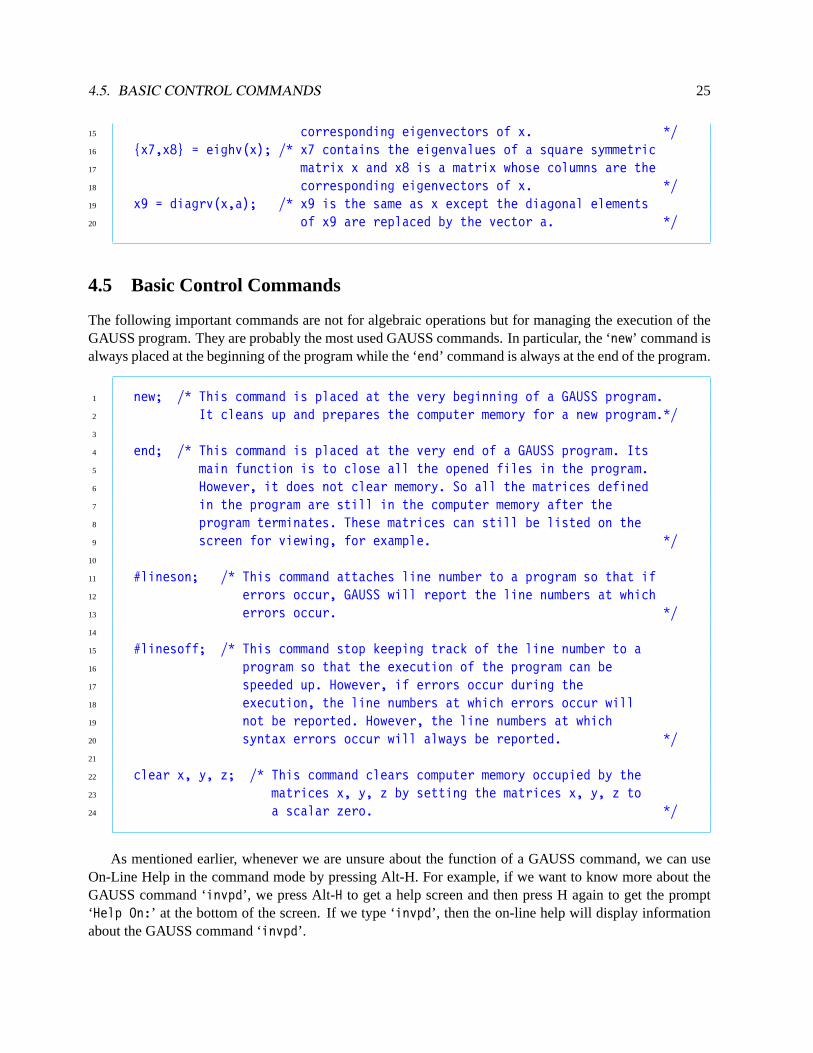
10 x2 = invpd(x); /* The inverse of the positive definite matrix x. */11 x3 = eig(x); /* The eigenvalues of a square matrix x. */12 x4 = eigh(x); /* The eigenvalues of a square symmetric matrix x. */13 {x5,x6} = eigv(x); /* x5 contains the eigenvalues of a square matrix x14 and x6is a matrix whose columns are the
4.5. BASIC CONTROL COMMANDS 25
15 corresponding eigenvectors of x. */16 {x7,x8} = eighv(x); /* x7 contains the eigenvalues of a square symmetric17 matrix x and x8 is a matrix whose columns are the18 corresponding eigenvectors of x. */19 x9 = diagrv(x,a); /* x9 is the same as x except the diagonal elements20 of x9 are replaced by the vector a. */
4.5 Basic Control Commands
The following important commands are not for algebraic operations but for managing the execution of theGAUSS program. They are probably the most used GAUSS commands. In particular, the ‘new’ command isalways placed at the beginning of the program while the ‘end’ command is always at the end of the program.
1 new; /* This command is placed at the very beginning of a GAUSS program.2 It cleans up and prepares the computer memory for a new program.*/3
4 end; /* This command is placed at the very end of a GAUSS program. Its5 main function is to close all the opened files in the program.6 However, it does not clear memory. So all the matrices defined7 in the program are still in the computer memory after the8 program terminates. These matrices can still be listed on the9 screen for viewing, for example. */
10
11 #lineson; /* This command attaches line number to a program so that if12 errors occur, GAUSS will report the line numbers at which13 errors occur. */14
15 #linesoff; /* This command stop keeping track of the line number to a16 program so that the execution of the program can be17 speeded up. However, if errors occur during the18 execution, the line numbers at which errors occur will19 not be reported. However, the line numbers at which20 syntax errors occur will always be reported. */21
22 clear x, y, z; /* This command clears computer memory occupied by the23 matrices x, y, z by setting the matrices x, y, z to24 a scalar zero. */
As mentioned earlier, whenever we are unsure about the function of a GAUSS command, we can useOn-Line Help in the command mode by pressing Alt-H. For example, if we want to know more about theGAUSS command ‘invpd’, we press Alt-H to get a help screen and then press H again to get the prompt‘Help On:’ at the bottom of the screen. If we type ‘invpd’, then the on-line help will display informationabout the GAUSS command ‘invpd’.
26 CHAPTER 4. GAUSS COMMANDS
4.6 Some Examples
It is possible to use GAUSS to verify many matrix algebra results and it is interesting to see how we canwrite GAUSS programs to do that.
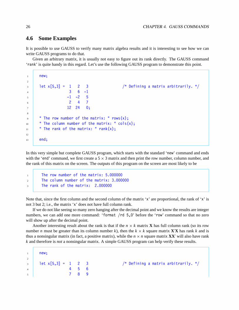
Given an arbitrary matrix, it is usually not easy to figure out its rank directly. The GAUSS command‘rank’ is quite handy in this regard. Let’s use the following GAUSS program to demonstrate this point.
1 new;2
3 let x[5,3] = 1 2 3 /* Defining a matrix arbitrarily. */4 3 6 -15 -1 -2 56 2 4 77 12 24 0;8
9 " The row number of the matrix: " rows(x);10 " The column number of the matrix: " cols(x);11 " The rank of the matrix: " rank(x);12
13 end;
In this very simple but complete GAUSS program, which starts with the standard ‘new’ command and endswith the ‘end’ command, we first create a 5× 3 matrix and then print the row number, column number, andthe rank of this matrix on the screen. The outputs of this program on the screen are most likely to be
1 The row number of the matrix: 5.0000002 The column number of the matrix: 3.0000003 The rank of the matrix: 2.000000
Note that, since the first column and the second column of the matrix ‘x’ are proportional, the rank of ‘x’ isnot 3 but 2; i.e., the matrix ‘x’ does not have full column rank.
If we do not like seeing so many zero hanging after the decimal point and we know the results are integernumbers, we can add one more command: ‘format /rd 5,0’ before the ‘row’ command so that no zerowill show up after the decimal point.
Another interesting result about the rank is that if then × k matrix X has full column rank (so its rownumbern must be greater than its column numberk), then thek × k square matrixX′X has rankk and isthus a nonsingular matrix (in fact, a positive matrix), while then × n square matrixXX ′ will also have rankk and therefore isnota nonsingular matrix. A simple GAUSS program can help verify these results.
1 new;2
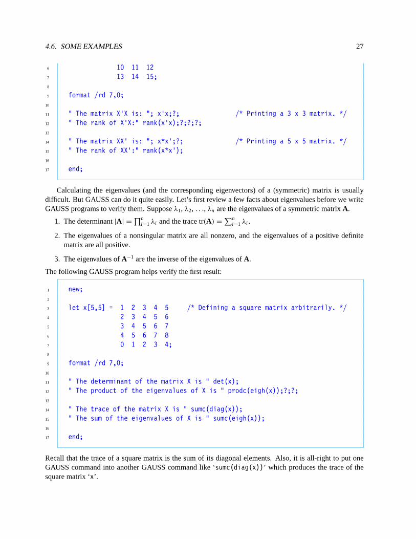
3 let x[5,3] = 1 2 3 /* Defining a matrix arbitrarily. */4 4 5 65 7 8 9
4.6. SOME EXAMPLES 27
6 10 11 127 13 14 15;8
9 format /rd 7,0;10
11 " The matrix X’X is: "; x’x;?; /* Printing a 3 x 3 matrix. */12 " The rank of X’X:" rank(x’x);?;?;?;13
14 " The matrix XX’ is: "; x*x’;?; /* Printing a 5 x 5 matrix. */15 " The rank of XX’:" rank(x*x’);16
17 end;
Calculating the eigenvalues (and the corresponding eigenvectors) of a (symmetric) matrix is usuallydifficult. But GAUSS can do it quite easily. Let’s first review a few facts about eigenvalues before we writeGAUSS programs to verify them. Supposeλ1, λ2, . . ., λn are the eigenvalues of a symmetric matrixA.
1. The determinant|A| =∏n
i =1 λi and the trace tr(A) =∑n
i =1 λi .
2. The eigenvalues of a nonsingular matrix are all nonzero, and the eigenvalues of a positive definitematrix are all positive.
3. The eigenvalues ofA−1 are the inverse of the eigenvalues ofA.
The following GAUSS program helps verify the first result:
1 new;2
3 let x[5,5] = 1 2 3 4 5 /* Defining a square matrix arbitrarily. */4 2 3 4 5 65 3 4 5 6 76 4 5 6 7 87 0 1 2 3 4;8
9 format /rd 7,0;10
11 " The determinant of the matrix X is " det(x);12 " The product of the eigenvalues of X is " prodc(eigh(x));?;?;13
14 " The trace of the matrix X is " sumc(diag(x));15 " The sum of the eigenvalues of X is " sumc(eigh(x));16
17 end;
Recall that the trace of a square matrix is the sum of its diagonal elements. Also, it is all-right to put oneGAUSS command into another GAUSS command like ‘sumc(diag(x))’ which produces the trace of thesquare matrix ‘x’.

28 CHAPTER 4. GAUSS COMMANDS
In the following program we will create a positive definite matrix using the fact that thek × k matrixX′X is always positive definite if then × k matrixX has full column rank.
1 new;2
3 let x[5,3] = 1 2 3 /* Defining a matrix of full column rank. */4 4 5 65 7 8 96 10 11 127 13 14 15;8
9 format /rd 10,6;10
11 " The eigenvalues of the positive definite matrix X’X and its inverse, ";12 " as well as the reciprocals of the latter:";13
14 eigh(x’x)˜eigh(invpd(x’x))˜(1./eigh(invpd(x’x)));15
16 end;
Since we use horizontal concatenation ‘˜’ to put together the three columns of results, a 3×3 matrix will beprinted and it should confirm that all the eigenvalues of ‘x’x’ are positive and that the eigenvalues of ‘x’x’and ‘invpd(x’x)’ are reciprocal.
Note that the last column is the result of element-by-element division ‘1./eigh(invpd(x’x))’. Thereason for an additional pair of parentheses to encircle this expression is to prevent the possibility that theconcatenation ‘’ may have higher priority in execution than the division, in which case the result would becompletely messed up. We should use parentheses generously to avoid any potential confusion of this kind.
Also note that we use the ‘invpd’ command, instead of the ‘inv’ command, to invert the matrix ‘x’x’because we know ‘x’x’ is positive definite. There are two advantages of using the ‘invpd’ command toinvert a positive definite matrices: First, the ‘invpd’ command can do the job more efficiently than ‘inv’,which is applicable to any nonsingular matrix. Secondly, if for whatever reason (e.g., ‘x’ does not havefull column rank) ‘x’x’ is not positive definite, GAUSS will not execute the ‘invpd(x’x)’ command andcomplain about it. This is good for detecting any potential problem of the program.
We now consider two results on the partitioned matrices. The first one involves an important formulafor inversion: [
A1 B
C A2
]−1
=
[X1 −A−1
1 BX2
−A−12 CX1 X2
],
whereX1 = (A1 − BA−1
2 C)−1 and X2 = (A2 − CA−11 B)−1,
andA1 andX1 are two square matrices of the same dimensions; andA2 andX2 are two square matrices ofthe same dimensions.
To write a GAUSS program to verify this result, we first define an arbitrary nonsingular 5× 5 matrix‘big_mac’, which consists of four blocks ‘a1’, ‘ b’, ‘ c’, and‘a2’.
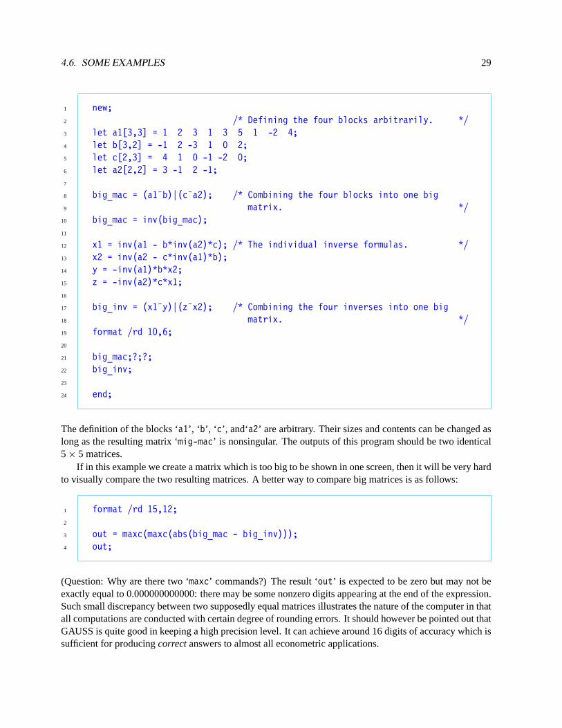
4.6. SOME EXAMPLES 29
1 new;2 /* Defining the four blocks arbitrarily. */3 let a1[3,3] = 1 2 3 1 3 5 1 -2 4;4 let b[3,2] = -1 2 -3 1 0 2;5 let c[2,3] = 4 1 0 -1 -2 0;6 let a2[2,2] = 3 -1 2 -1;7
8 big_mac = (a1˜b)|(c˜a2); /* Combining the four blocks into one big9 matrix. */
10 big_mac = inv(big_mac);11
12 x1 = inv(a1 - b*inv(a2)*c); /* The individual inverse formulas. */13 x2 = inv(a2 - c*inv(a1)*b);14 y = -inv(a1)*b*x2;15 z = -inv(a2)*c*x1;16
17 big_inv = (x1˜y)|(z˜x2); /* Combining the four inverses into one big18 matrix. */19 format /rd 10,6;20
21 big_mac;?;?;22 big_inv;23
24 end;
The definition of the blocks ‘a1’, ‘ b’, ‘ c’, and‘a2’ are arbitrary. Their sizes and contents can be changed aslong as the resulting matrix ‘mig-mac’ is nonsingular. The outputs of this program should be two identical5 × 5 matrices.
If in this example we create a matrix which is too big to be shown in one screen, then it will be very hardto visually compare the two resulting matrices. A better way to compare big matrices is as follows:
1 format /rd 15,12;2
3 out = maxc(maxc(abs(big_mac - big_inv)));4 out;
(Question: Why are there two ‘maxc’ commands?) The result ‘out’ is expected to be zero but may not beexactly equal to 0.000000000000: there may be some nonzero digits appearing at the end of the expression.Such small discrepancy between two supposedly equal matrices illustrates the nature of the computer in thatall computations are conducted with certain degree of rounding errors. It should however be pointed out thatGAUSS is quite good in keeping a high precision level. It can achieve around 16 digits of accuracy which issufficient for producingcorrectanswers to almost all econometric applications.

30 CHAPTER 4. GAUSS COMMANDS
Note that the above formula for the inverse of the partitioned matrix involves the inverses of the twodiagonal blocksA1 andA2. It is sometimes possible that one of them may not be invertible, say,A2, inwhich case we should replace the two sub-formulasX1 = (A1−BA−1
2 C)−1 and−A−12 CX1 by the equivalent
A−11 + A−1
1 BX2CA−11 and−X2CA−1
1 , respectively.Let’s now consider two formulas for the determinant of the partitioned matrix:∣∣∣∣∣A1 B
C A2
∣∣∣∣∣ = |A2|·|A1 − BA−12 C| = |A1|·|A2 − CA−1
1 B|.
The corresponding GAUSS program for checking the first equality is
1 new;2
3 let a1[3,3] = 1 2 3 1 3 5 1 -2 4;4 let b[3,2] = -1 2 -3 1 0 2;5 let c[2,3] = 4 1 0 -1 -2 0;6 let a2[2,2] = 3 -1 2 -1;7
8 one_det = det((a1˜b)|(c˜a2));9 two_det = det(a2)*det(a1 - b*inv(a2)*c);
10 out = abs(one_det - two_det);11
12 format /rd 15,12;13 out;14
15 end;
The above formulas for the partitioned matrices are very useful when we need the inverse or the de-terminant of a big matrix while the computer memory is not sufficient to handle it. These examples alsodemonstrate an important trick in dealing with the problem of insufficient memory: we can and should breakthe trouble-making matrix into smaller pieces and handle them piece by piece.
Let’s now use the International Consumption Data to construct additional examples. Given quantitiesqic
and budget sharessic for the commodityi in countryc, and the country c’s incomemc for the 60 countries,we can reorderqic andsic according to their income, either in ascending or descending order:
1 new;2
3 load q[60,10] = a:\data\volume; /* The quantities. */4 load s[60,10] = a:\data\share; /* The budget shares. */5 load m[60,1] = a:\data\totalexp; /* The total expenditure. */6
7 q = sortc(m˜q,1);8 s = sortc(m˜s,1);9

4.6. SOME EXAMPLES 31
10 output file = order.out on;11 format /rd 10,3;;12
13 " The Ordered Income and Quantities (in Ascending Order):";14 q;?;15 " The Ordered Income and Budget Shares (in Ascending Order):";16 s;?;?;?;17
18 " The Ordered Income and Quantities (in Descending Order):";19 rev(q);?;20 " The Ordered Income and Budget Shares (in Descending Order):";21 rev(s);22
23 end;
Four 60× 11 matrices will be printed into the ASCII file ‘order.out’. The first two matrices are orderedin the ascending order of the first column, which is the column of income. The last two matrices are inthe descending order of the income. It is interesting to see that the Food budget share increases as incomedecreases.
We can compute many summary statistics for the International Consumption Data. Specifically, wecan calculate the averages, sample medians, standard deviations, maxima, minima, and with a little morealgebra, the sample covariances and correlation coefficients.
Let’s concentrate on the sample covariances and correlation coefficients betweenmc and eachsic, i =
1, . . . ,10, which are
Cov(si ,m) =1
60
60∑c=1
(sic − si )(mc − m) and Corr(si ,m) =Cov(si ,m)√
Var(si ) ·
√Var(m)
,
respectively, wheresi andm are the sample averages andVar(si ) andVar(m) are the sample variances:
Var(si ) =1
60
60∑c=1
(sic − si )2 and Var(m) =
1
60
60∑c=1
(mc − m)2.
SupposeS is the 60× 10 matrix of data onsic, andm is the 60× 1 vector of data onmc. We can construct a60× 10 matrixS in which each column contains 60 identical numbers which are the sample averages of thebudget shares. Thus, the(i, c)-th element of the difference matrixD = S− S is preciselysic − si . We cansimilarly define a vectora whose typical element is the differencemc − m. Given these definitions, we thenhave
D′a = [ d1 d2 · · · d10 ]′a =
d′
1
d′
2
...
d′
10
a =
d′
1a
d′
2a
...
d′
10a
,

32 CHAPTER 4. GAUSS COMMANDS
which is a 10× 1 vector with thei th element being the sample covariance between thei th budget sharesi
and incomem:
d′
i a =
60∑c=1
dicac =
60∑c=1
(sic − si )(mc − m), i = 1, . . . ,10.
This formula can be adopted for efficiently computing the sample covariances in GAUSS. Given that ‘s’denotesS and ‘m’ denotesm in GAUSS, if we define
1 cov_sm = (s - meanc(s)’)’(m - meanc(m))./60;
then ‘cov_sm’ is a 10× 1 vector of sample covariances betweensic andmc, for i = 1, . . . ,10. Here, weshould note that ‘meanc(s)’ gives a 10× 1 vector of means and its dimension is not the same as ‘s’. But‘s - meanc(s)’’ will correctly produce the matrixD = S− S because the particular way GAUSS handlessubtraction of matrices of unequal sizes. This is a useful trick and it can be used in many occasions.
We can similarly compute the two sample variances ofsic andmc as follows:
1 varcov_s = (s - meanc(s)’)’(s - meanc(s)’)./60;2 var_s = diag(varcov_s);3 var_m = (m - meanc(m)’)’(m - meanc(m)’)./60;
Note that ‘varcov_s’ is a 10× 10 sample variance-covariance matrix ofsic, c = 1,2, . . . ,10, and itsdiagonal contains 10 sample variances. Also note that GAUSS provides us with a command ‘stdc’ whichcomputes the standard deviation (the square root of the sample variance). That is, the vectors ‘var_s’should be equal to ‘stdc(s)ˆ2’, and ‘var_m’ should be equal to ‘stdc(m)ˆ2’. Therefore, the correlationcoefficients can be computed by either
1 corr_sm = cov_sm./sqrt(var_s.*var_m);
where ‘var_s’ and ‘var_m’ are computed as above, or, equivalently,
1 corr_sm = cov_sm./(stdc(s).*stdc(m));
Note that the sizes of the matrices ‘cov_sm’, ‘ var_s’, ‘ var_m’, and ‘corr_sm’ are all 10.We now combine all these expressions in one GAUSS program to generate the basic summary statistics
for the International Consumption Data. Here, instead of looking at total expendituremc, we consider theln mc, the logarithmic transformation ofmc. The GAUSS command for the natural log transformation is‘ln’.
1 new;2
3 load q[60,10] = a:\data\volume;4 load s[60,10] = a:\data\share;5 load m[60,1] = a:\data\totalexp;

4.6. SOME EXAMPLES 33
6
7 m = ln(m); /* The log total expenditure. */8
9 p = (m.*s)./q; /* The prices. */10
11 mean_s = meanc(s); /* The averages. */12 mean_m = meanc(m);13 mean_p = meanc(p);14
15 std_s = stdc(s); /* The standard deviations. */16 std_m = stdc(m);17 std_p = stdc(p);18
19 /* The sample covariances between shares and log total expenditure. */20 cov_sm = (s - mean_s’)’(m - mean_m)./60;21
22 /* The sample correlations between shares and log total expenditure. */23 corr_sm = cov_sm./(std_s.*std_m);24
25 /* The sample covariances between prices and log total expenditure. */26 cov_pm = (p - mean_p’)’(m - mean_m)./60;27
28 /* The sample correlations between prices and log total expenditure. */29 corr_pm = cov_pm./(std_p.*std_m);30
31 /* Creating a vector of consecutive numbers from 1 to 10. */32 no = seqa(1,1,10);33
34 out_s = no˜mean_s˜std_s˜maxc(s)˜minc(s)˜median(s)˜cov_sm˜corr_sm;35 out_p = no˜mean_p˜std_p˜maxc(p)˜minc(p)˜median(p)˜cov_pm˜corr_pm;36 out_m = mean_m˜std_m˜maxc(m)˜minc(m)˜median(m);37
38 output file = summary on;39 format /rd 7,3;40
41 " The sample averages, standard deviations, maxima, minima, medians, "42 " of shares; and the sample covariances and the sample correlations "43 " between shares and log total expenditure:";44 out_s;?;?;45
46 " The sample averages, standard deviations, maxima, minima, medians, "47 " of prices; and the sample covariances and the sample correlations "48 " between prices and log total expenditure:";49 out_p;?;?;50

34 CHAPTER 4. GAUSS COMMANDS
51 " The sample averages, standard deviations, maxima, minima, and medians "52 " of the log total expenditure:";53 out_m;54
55 end;
The ‘no’ vector is constructed as a counting device to facilitate the reading of the outputs.Finally, it should be pointed out that there are GAUSS commands ‘vcx(s)’ and ‘corrx(s)’ which
compute the 10× 10 variance-covariance matrix and the correlation matrix, respectively, from the 60× 10data matrix ‘s’. The diagonal terms of ‘vcx(s)’ are sample variances while the off-diagonal elements aresample covariances. Also, the diagonal terms of ‘corrx(s)’ are all ones. The two matrices ‘cov_sm’ and‘corr_sm’ in the previous program will then be equal to the last columns (except the last elements) of theresulting matrices from ‘vcx(s˜m)’ and ‘corrx(s˜m)’, respectively.
4.7 Character Matrices and Strings
Other than numeric data, GAUSS also allows character data which may be presented in two forms: charactermatrices and strings.
4.7.1 Character Matrices
The most common form of the character matrix is the character vector, which are used mainly for storing avector of names for the purpose of identifying rows or columns of a numeric data matrix. For example, an1× k character row vector can be created and then concatenated to ann × k matrix of numbers so that eachcolumn ofn numbers can be associated with a character name. Consider a more specific example: Supposethe 60× 10 matrix ‘s’ contains 60 observations on 10 budget shares. We can store the names of the 10commodity into a 1×10 character vector, say, ‘varname’, and concatenate this row vertically to the numericmatrix ‘s’ as follows:
1 let varname[1,10] = Food B_T Cloth Rent House2 Medic Trans Recre Ed Other;3
4 s1 = varname|s;
Here, ‘s1’ is a 61× 10 mixed matrix in which the first row are characters and the rest are numbers.From this simple example we know the way characters are stored in a vector is quite similar to that
of a numeric matrix. However, there are a few more rules for handling character vectors: each elementof a character vector can contain up to eight characters only. The contents of the above character vector‘varname’ will all be uppercase, such as ‘FOOD’ instead of ‘Food’. If the cases of the characters are to bekept exactly as what they are typed, such as ‘Food’, then they need to be enclosed by quotation marks in the‘let’ command as follows:
1 let varname[1,10] = "Food" "B_T" "Cloth" "Rent" "House"2 "Medic" "Trans" "Recre" "Ed" "Other";
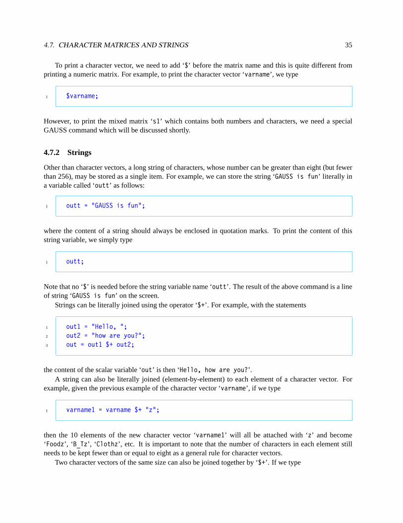
4.7. CHARACTER MATRICES AND STRINGS 35
To print a character vector, we need to add ‘$’ before the matrix name and this is quite different fromprinting a numeric matrix. For example, to print the character vector ‘varname’, we type
1 $varname;
However, to print the mixed matrix ‘s1’ which contains both numbers and characters, we need a specialGAUSS command which will be discussed shortly.
4.7.2 Strings
Other than character vectors, a long string of characters, whose number can be greater than eight (but fewerthan 256), may be stored as a single item. For example, we can store the string ‘GAUSS is fun’ literally ina variable called ‘outt’ as follows:
1 outt = "GAUSS is fun";
where the content of a string should always be enclosed in quotation marks. To print the content of thisstring variable, we simply type
1 outt;
Note that no ‘$’ is needed before the string variable name ‘outt’. The result of the above command is a lineof string ‘GAUSS is fun’ on the screen.
Strings can be literally joined using the operator ‘$+’. For example, with the statements
1 out1 = "Hello, ";2 out2 = "how are you?";3 out = out1 $+ out2;
the content of the scalar variable ‘out’ is then ‘Hello, how are you?’.A string can also be literally joined (element-by-element) to each element of a character vector. For
example, given the previous example of the character vector ‘varname’, if we type
1 varname1 = varname $+ "z";
then the 10 elements of the new character vector ‘varname1’ will all be attached with ‘z’ and become‘Foodz’, ‘ B_Tz’, ‘ Clothz’, etc. It is important to note that the number of characters in each element stillneeds to be kept fewer than or equal to eight as a general rule for character vectors.
Two character vectors of the same size can also be joined together by ‘$+’. If we type

36 CHAPTER 4. GAUSS COMMANDS
1 let a[3,1] = "GAUSS" "is" "fun";2 let b[3,1] = "So" "is" "Econ";3
4 c = a $+ b;
then ‘c’ is also a 3× 1 vector with the three elements: ‘GAUSSSo, isis, andfunEcon.
4.7.3 The Data Type
It is important to understand that strings, as opposed to other data formats such as numeric matrices orcharacter vectors, are a very uniquetypeof data. As a matter of fact, all data in GAUSS can be broadlyclassified as of eitherstring typeor matrix type, while both numeric matrices and character vectors belongto the matrix type. The difference between the string type and the matrix type can be best illustrated in thefollowing problematic statement which invokes the error message of ‘Type Mismatch’:
1 varname2 = "z" $+ varname;
where ‘varname’ is a 10× 1 character vector as defined above. The problem results from a rule in GAUSSthat thetypeof the right-hand side operation is decided by thetypeof the first item. In the above example,the first item ‘z’ on the right-hand side is a string, so the joint operation is considered to be an operationamong strings and every item at the right-hand side is expected to be a string. But since the second item isactually a matrix, the syntax error of mismatched type will show up. To fix this problem, we can adopt thefollowing trick:
1 varname2 = 0 $+ "z" $+ varname;
Here, the first item ‘0’ on the right-hand side is a number, which is always of the matrix type. So theentire operation on the right-hand side is considered a matrix operation and ‘z’ is treated as a matrix with asingle element instead of a string (the usual element-by-element rule is then applied to the ‘$+’ operations).After the characters are joined, the elements of the character vector ‘varname2’ become ‘zFood’, ‘ zB_T’,‘zCloth’, etc. Note that the value 0 itself will not be a part of the characters.
4.7.4 Three Useful GAUSS Commands
A couple of problems may arise when we try to combine numeric matrices with character vectors:
1. In many occasions we may want to combine a character vector and a numeric vector to create anothercharacter vector of which each entry mixes characters with numbers. But we note characters andnumbers are of different nature and we are not sure whether the character joint operator ‘$+’ can beapplied to combine characters and numbers.
2. When we print a character vector, we have to precede its variable name with a dollar sign ‘$’ in theprint command. It is then unclear how to print a matrix that contains both numbers and characters.

4.7. CHARACTER MATRICES AND STRINGS 37
To solve the first problem of jointing numbers with characters or with strings, we use the commands‘ftocv’ or ‘ ftos’ to convert numbers to characters or to strings, respectively. As to the problem of printinga mixed matrix containing both numbers and characters, we need the ‘printfm’ command. These threecommands will now be discussed in details.
1. The ‘ftocv’ command converts a numeric vector (or matrix) to a character vector. Given a vector‘a’ of real numbers, if we want to convert it to a character vector with each element containing 7characters in which 2 digits after the decimal point as well as the decimal point itself will all appearas characters, we type
1 b = ftocv(a,7,2);
The ‘b’ vector now is a character vector,even though its contents look like numbers, and can be joinedwith any other character vector. If a number is not large enough to fill the space of 7 characters,character 0 will be padded on the left. Also, if we do not want the decimal point and the digits after itto be converted, we replace 2 in the third input of the ‘ftocv’ command by 0.
Consider another example
1 name = 0 $+ "Var" $+ ftocv(seqa(0,1,21),1,0);
Here, a sequence of 21 consecutive integers starting from 1 are first generated by the ‘seqa(0,1,21)’command and then converted to a 21× 1 character vector by the ‘ftocv’ command. This charactervector is then joined to the string ‘Var’. The resulting ‘name’ is a 21× 1 character vector containingthe characters ‘Var1’, ‘ Var2’, . . . Note that the trick of ‘0 $+’ at the right-hand side is used to preventthe ‘Type Mismatch’ problem (see the previous subsection).
2. The ‘ftos’ command converts a scalar to a string. Given a real numbers ‘a’, if we want to convert itto a string of 15 characters in which 4 digits after the decimal point will be included, we type
1 b = ftos(a,"%*.*lf",15,4);
In comparison with the ‘ftocv’ command, we note the ‘ftos’ command has four inputs. The defini-tions of the first, third, and the fourth inputs are the same as the three inputs of the ‘ftocv’ command,respectively. The second input should be a string enclosed in quotation marks. The specific string‘%*.*lf’ here will direct GAUSS to right-justify the characters. If ‘a’ is not large enough to fill thespace of 15 characters, space (instead of character 0) will be padded on the left. Another commonspecification is ‘%-*.*lf’, which left-justifies the characters. Moreover, there is a simple way to addother characters literally before and after the character representation of the number: we put thesecharacters inside the quotation marks before and/or after ‘%*.*lf’. For example, if the value of ‘a’ is1234.567890123 and we type
1 b = ftos(a,"This Trial Produces %*.*lf, Which Are Characters.",12,4);

38 CHAPTER 4. GAUSS COMMANDS
then ‘b’ will be a string with the content:
1 This Trial Produces 1234.5678, Which Are Characters.
3. The ‘printfm’ command provides us with the full control on how to print data in a matrix wheresome columns are numbers and some are characters. In particular, different columns can be printed indifferent formats. Suppose we want to print an 10× 5 matrix ‘x’ in which the first column containscharacters and the rest all numbers, then we type:
1 indx = zeros(10,1)˜ones{10,4);2
3 let c[5,3] = "%*.*s" 10 104 "%*.*lf" 12 45 "%*.*lf" 8 26 "%-*.*lf" 10 37 "%-*.*lf" 6 0;8
9 ok = printfm(x,indx,c);
Here, the matrix ‘indx’ has the same dimension as ‘x’ and contains 1 and 0 only. When an element of‘x’ is a number, then the corresponding element in the ‘indx’ matrix must be the number 1, but if theelement of ‘x’ is a character, then the corresponding element in the ‘indx’ matrix must be the number0. It is possible to make ‘indx’ a 1 × 5 row vector containing the five numbers 0, 1, 1, 1, and 1. Insuch a case, the usual element-by-element operation will be applied.
As to the matrix ‘c’, its row number must be the same as thecolumnnumber of the data matrix ‘x’.This is because thei -th row in ‘c’ specifies the format for thei -th column of ‘x’. The first elementin each row of the ‘c’ matrix is a string. Its content usually is one of ‘%*.*lf’, ‘ %-*.*lf’, ‘ %*.*s’,‘%-*.*s’, where the first two are exactly the same as the second input of the ‘ftos’ command andtheir interpretations are also the same. Note that ‘%*.*lf’ can be abbreviated as ‘lf’. As to the lasttwo commands that contain the character ‘s’, they are for character printing.
The second and the third elements in each row of the ‘c’ matrix specify the number of spaces reservedfor printing and the number of digits after the decimal point, respectively. They work like what thesecond and the third inputs of the ‘ftocv’ command.
It is possible for some column of the ‘x’ matrix to have both numbers and characters at the same time.In such cases the corresponding rows in the ‘c’ matrix should still be either ‘%*.*lf’ or ‘ %-*.*lf’.When characters are encountered in printing the column, GAUSS will print them appropriately (aslong as the 0-1 specifications in the second input matrix ‘indx’ are correct).
The output of the ‘printfm’ command ‘ok’ is either 1 or 0, depending on whether printing is success-ful or not. If this information is not needed, we can type
1 call printfm(x,indx,c);

4.7. CHARACTER MATRICES AND STRINGS 39
Note that the command ‘?;’ should be included after the above command. Otherwise, the next thingto be printed will immediately follow the last line of ‘x’, instead of starting from a new line.

40 CHAPTER 4. GAUSS COMMANDS

Chapter 5GAUSS Program for Linear Regression
In this chapter we will write a GAUSS program for the Ordinary Least Squares (OLS) estimation of a linearregression model after a brief review of the linear regression theory. A full discussion of such a theory canbe found in any intermediate econometrics textbook.
5.1 A Brief Review
Givenn observations on the dependent variableyi andk explanatory variables (regressors)x1i , . . . , xki , weconsider the following linear regression model
yi = β1x1i + β2x2i + · · · + βkxki + εi , i = 1, , . . . , n,
which can be expressed compactly in matrix form:
yn×1
= Xn×k
βββk×1
+ εεεn×1
or
y1
y1
...
yn
=
x11 x21 · · · xk1
x12 x22 · · · xk2
......
...
x1n x2n · · · xkn
β1
β2
...
βk
+
ε1
ε2
...
εn
,
whereβ1, β2, . . ., βk arek regression coefficients andεi are the random disturbance terms. Four assumptionsare usually made about the disturbance terms (1) E(εεε) = 0; (2) Var(εεε) = σ 2In, whereIn is ann × n identitymatrix; (3)εi is normally distributed; and (4)X is nonstochastic and is of full column rank, i.e., rank(X) = k.Note that the second assumption implies the disturbance terms are homoscedastic and unautocorrelated. Itis also common to assume that one of the explanatory variables is a constant term. So one column of thematrixX (usually the first column) is a column of ones.
5.1.1 The Ordinary Least Squares Estimation
The OLS estimator of the parameterβββ is defined as
b = (X′X)−1X′y, (5.1)
whereX′X is invertible (and positive definite) becauseX is assumed to be of full column rank. It can also beshown that the OLS estimatorb is the BLUE (best linear unbiased estimator) andb ∼ N (βββ, σ 2(X′X)−1).The result thatb is normally distributed is due to the normality assumption on the disturbance terms.
Given the residualse = y − Xb, (5.2)
41

42 CHAPTER 5. GAUSS PROGRAM FOR LINEAR REGRESSION
the unbiased estimator of the disturbance varianceσ 2 is
s2=
1
n − ke′e. (5.3)
The variance-covariance matrix of the OLS estimator Var(b) = σ 2(X′X)−1 can be estimated by
Var(b) = s2(X′X)−1. (5.4)
The square root of thej -th diagonal element of (5.4)
s.e.(b j ) =
√s2(X′X)−1
j j , for j = 1, . . . , k., (5.5)
is the standard errors of thej -th OLS estimatorb j and the corresponding t-ratio is
t j =b j
s.e.(b j ). (5.6)
If the true value ofβ j is zero, thent j has a t-distribution withn − k degrees of freedom. This result can beused to test the hypothesis
H0: β j = 0 against H1: β j 6= 0,
and to construct the confidence interval forb j atα level which is
b j ± tα/2(n − k)× s.e.(b j ), (5.7)
wheretα/2(n − k) is theα/2 level critical value from the t-distribution withn − k degrees of freedom.
5.1.2 Analysis of Variance
The total sample variations in the dependent variable is usually measured by the Total Sum of Squares(TSS):
TSS=
n∑i =1
(yi − y)2 = (y − y·1n)′(y − y·1n). (5.8)
where1n is an n-dimensional column of ones. We note that TSS is simply the sample variance ofyi
multiplied by the sample size. Based on the linear regression model we can decompose the TSS into twoparts: the part of variations that can bepredictedor explainedby a linear combination of explanatoryvariables is called the Explained Sum of Squares (ESS), while the other part is called the Residual Sumof Squares (RSS). The RSS is generally easier to compute because it equals
RSS=
n∑i =1
e2i = e′e, (5.9)
which measures the variations in the residuals. ESS can be calculated by subtraction:
ESS= TSS− RSS. (5.10)
A little more algebra can yield some other expressions for ESS. Here, let’s concentrate on its interpretation.

5.1. A BRIEF REVIEW 43
The linear regression model is based on the idea that the variations in the dependent variableyi dependslinearly on those of explanatory variablesx1i , x1i , . . ., xki . Hence, the performance of a linear regressionmodel can be measured by the proportion of the variations in the dependent variables that can beexplainedbythe variations in the linear combination of explanatory variables. Such a proportion is called the coefficientof determination or simply R2:
R2=
ESS
TSS= 1 −
RSS
TSS. (5.11)
It is the most common measure of the goodness-of-fit of a linear regression model. Its value lies between 0and 1 and the larger its value the better. However, there is a problem with the R2 measure: its value can beincreased superficially by including even the most irrelevant explanatory variable into the model. To avoidthis problem, we can modify R2 by making the number of explanatory variables as a counterweight. Moreprecisely, we have the following definition of the adjusted R2:
R2
= 1 −RSS/(n − k)
TSS/(n − 1)= 1 −
n − 1
n − k(1 − R2), (5.12)
whose value can decrease when we add into the model an explanatory variable that has very little contribu-tion in explaining the dependent variable.
Based on ESS and RSS, let’s define the following two ratios which are called Explained Mean Square(EMS) and Residual Mean Square (RMS):
EMS =1
k − 1ESS and RMS=
1
n − kRSS.
Note that RMS is the same ass2 defined in(5.3).Given the normality assumption (the third assumption) on the disturbance terms, it can be shown that
the RSS/σ 2 has aχ2 distribution withn − k degrees of freedom. Furthermore, when the first explanatoryvariable is a constant term, then the ESS/σ 2 has aχ2 distribution withk − 1 degrees of freedom, and isindependent of the RSS/σ 2 if the coefficientsβ2, . . . , βk are all zero. As a result, the ratio
F =EMS
RMS, (5.13)
has anF-distribution withk − 1 andn − k degrees of freedom and can be used to test the hypothesis
H0: β2 = 0, · · · , βk = 0 against H1: β2 6= 0, · · · , βk 6= 0.
We can present all these results in a table:
5.1.3 Durbin-Watson Test Statistic
As mentioned earlier, the third assumption underlying the linear regression model implies the absence ofautocorrelation among the disturbance terms. But for time-series data this assumption usually fails to holdand it is quite common that the disturbance terms follow a first-order autoregressive, or the AR(1), process,which is defined by
εi = ρ εi −1 + ui ,
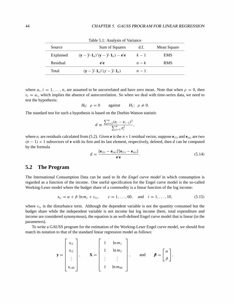
44 CHAPTER 5. GAUSS PROGRAM FOR LINEAR REGRESSION
Table 5.1: Analysis of Variance
Source Sum of Squares d.f. Mean Square
Explained (y − y·1n)′(y − y·1n)− e′e k − 1 EMS
Residual e′e n − k RMS
Total (y − y·1n)′(y − y·1n) n − 1
whereui , i = 1, . . . ,n, are assumed to be uncorrelated and have zero mean. Note that whenρ = 0, thenεi = ui , which implies the absence of autocorrelation. So when we deal with time-series data, we need totest the hypothesis:
H0: ρ = 0 against H1: ρ 6= 0.
The standard test for such a hypothesis is based on the Durbin-Watson statistic
d ≡
∑ni =2(ei − ei −1)
2∑ni =1 e2
i
,
whereei are residuals calculated from (5.2). Givene is then×1 residual vector, supposee(1) ande(n) are two(n − 1)× 1 subvectors ofe with its first and its last element, respectively, deleted, thend can be computedby the formula
d =[e(1) − e(n)]′[e(1) − e(n)]
e′e. (5.14)
5.2 The Program
The International Consumption Data can be used to fitthe Engel curve modelin which consumption isregarded as a function of the income. One useful specification for the Engel curve model is the so-calledWorking-Leser model where the budget share of a commodity is a linear function of the log income:
sic = α + β ·ln mc + εic, c = 1, . . . ,60, and i = 1, . . . ,10, (5.15)
whereεic is the disturbance term. Although the dependent variable is not the quantity consumed but thebudget share while the independent variable is not income but log income (here, total expenditure andincome are considered synonymous), the equation is an well-defined Engel curve model that is linear (in theparameters).
To write a GAUSS program for the estimation of the Working-Leser Engel curve model, we should firstmatch its notation to that of the standard linear regression model as follows:
y =
si 1
si 2
...
si,60
, X =
1 lnm1
1 lnm2
......
1 lnm60
, and βββ =
[α
β
].

5.2. THE PROGRAM 45
In the following GAUSS program the Food consumption data are used to estimate the Working-LeserEngel curve model. The first section of the program illustrates how the Food consumption data can beloaded into the appropriate matrices for computation. This GAUSS program produces standard output forthe linear regression estimation. Generally, we need to change the first four statements only and the rest canbe left as they are.
1 new;2
3 /*************************************************************************4 * Reading and Organizing the Data Set *5 *************************************************************************/6
7 load share[60,10] = a:\data\share;8 load totalexp[60,1] = a:\data\totalexp;9
10 y = share[.,1]; /* Forming the vector of the dependent11 variable which contains the budget share12 for Food. */13
14 x = ones(60,1)˜ln(totalexp); /* Forming the matrix for the two15 explanatory variables: the constant term16 and log income. */17
18 clear share, totalexp; /* Clearing the matrices that are no longer19 needed. */20
21 output file = ols.out reset; /* Defining the output file name as ols.out.*/22
23 /************************************************************************24 * Regression Estimation *25 ************************************************************************/26
27 n = rows(y); /* The sample size. */28 k = cols(x); /* The number of explanatory variables. */29
30 b = invpd(x’x)*x’y; /* (5.1) */31 e = y - x*b; /* (5.2) */32 s2 = e’e/(n-k); /* (5.3) */33 vb = s2.*invpd(x’x); /* (5.4) */34 seb = sqrt(diag(vb)); /* (5.5) */35 tb = b./seb; /* (5.6) */36
37 tss = (y - meanc(y))’(y - meanc(y)); /* (5.8) */38 rss = e’e; /* (5.9) */39 ess = tss - rss; /* (5.10) */
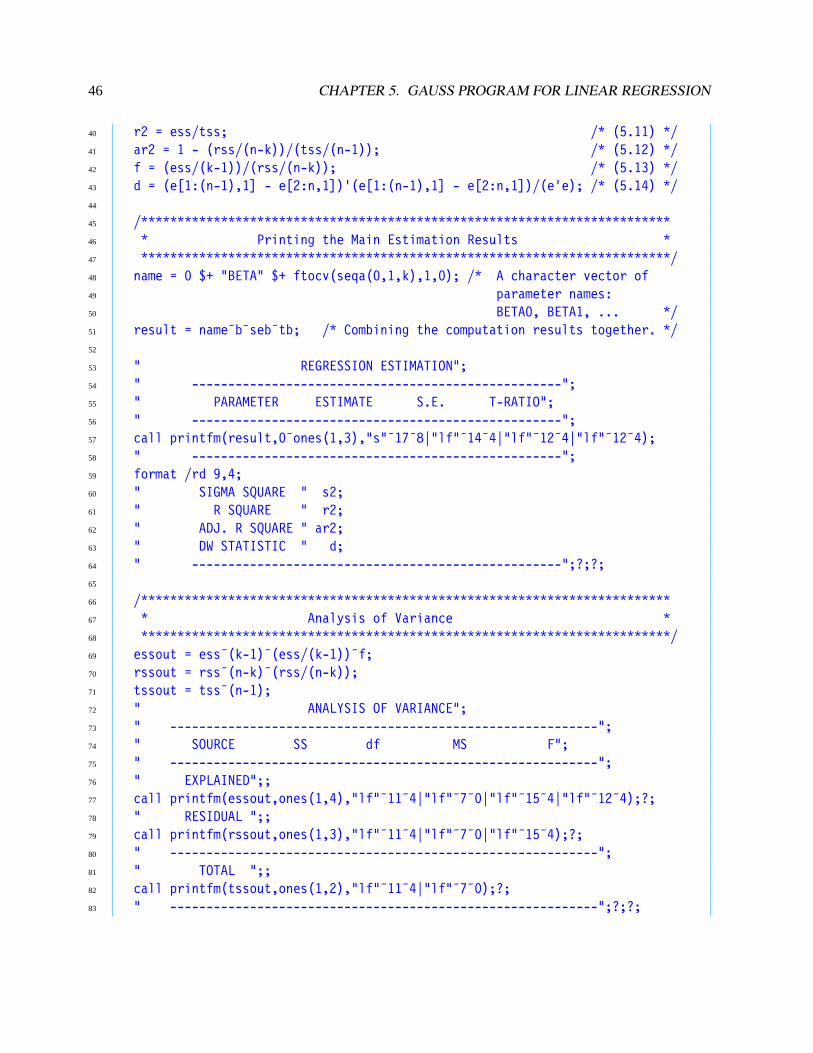
46 CHAPTER 5. GAUSS PROGRAM FOR LINEAR REGRESSION
40 r2 = ess/tss; /* (5.11) */41 ar2 = 1 - (rss/(n-k))/(tss/(n-1)); /* (5.12) */42 f = (ess/(k-1))/(rss/(n-k)); /* (5.13) */43 d = (e[1:(n-1),1] - e[2:n,1])’(e[1:(n-1),1] - e[2:n,1])/(e’e); /* (5.14) */44
45 /*************************************************************************46 * Printing the Main Estimation Results *47 *************************************************************************/48 name = 0 $+ "BETA" $+ ftocv(seqa(0,1,k),1,0); /* A character vector of49 parameter names:50 BETA0, BETA1, ... */51 result = name˜b˜seb˜tb; /* Combining the computation results together. */52
53 " REGRESSION ESTIMATION";54 " ---------------------------------------------------";55 " PARAMETER ESTIMATE S.E. T-RATIO";56 " ---------------------------------------------------";57 call printfm(result,0˜ones(1,3),"s"˜17˜8|"lf"˜14˜4|"lf"˜12˜4|"lf"˜12˜4);58 " ---------------------------------------------------";59 format /rd 9,4;60 " SIGMA SQUARE " s2;61 " R SQUARE " r2;62 " ADJ. R SQUARE " ar2;63 " DW STATISTIC " d;64 " ---------------------------------------------------";?;?;65
66 /*************************************************************************67 * Analysis of Variance *68 *************************************************************************/69 essout = ess˜(k-1)˜(ess/(k-1))˜f;70 rssout = rss˜(n-k)˜(rss/(n-k));71 tssout = tss˜(n-1);72 " ANALYSIS OF VARIANCE";73 " -----------------------------------------------------------";74 " SOURCE SS df MS F";75 " -----------------------------------------------------------";76 " EXPLAINED";;77 call printfm(essout,ones(1,4),"lf"˜11˜4|"lf"˜7˜0|"lf"˜15˜4|"lf"˜12˜4);?;78 " RESIDUAL ";;79 call printfm(rssout,ones(1,3),"lf"˜11˜4|"lf"˜7˜0|"lf"˜15˜4);?;80 " -----------------------------------------------------------";81 " TOTAL ";;82 call printfm(tssout,ones(1,2),"lf"˜11˜4|"lf"˜7˜0);?;83 " -----------------------------------------------------------";?;?;

5.2. THE PROGRAM 47
84 end;
The estimation results will be printed on the screen and into the ASCII file ‘ols.out’. Since there are morethan one screenful of the results, we have to use the editor to go into the output fileols.out to view thecomplete results.
An important feature of the above GAUSS program is that the OLS estimation is conducted in a way thatis independent of the data it processes. In other words, all we have to do for different applications is to loadthe appropriate data into the matrices ‘y’ and ‘x’, while the main body of the program can be used repeatedlywithout any modification. This structure of the program demonstrates the power of GAUSS programming.Once a program proves to work well, all the future applications can be made with minimum revisions. Toillustrate this point, let’s consider another OLS estimation based on the International Consumption Data, inwhich we extend the Engel curve model by including price terms to get the followingdemand model:
sic = β1 + β2 ln mc + β3 ln p1c + · · · + β12 ln p10,c + εic, c = 1, . . . ,60, (5.16)
where lnpic, i = 1, . . . ,10, are the log prices of the 10 commodities. In such a linear demand model thematrix X includes 12 columns of data: the constant term, the log income, and the 10 log prices. The vectorβββ contains 12 regression coefficients.
X =
1 lnm1 ln p11 · · · ln p10,1
1 lnm2 ln p12 · · · ln p10,2
......
......
1 lnm60 ln p1,60 · · · ln p10,60
and βββ =
β1
β2
...
β12
.
To estimate such a linear regression model, all we have to do is to rewrite the first part of the above programas follows:
1 load q[60,10] = a:\data\volume;2 load s[60,10] = a:\data\share;3 load m[60,1] = a:\data\totalexp;4
5 p = (m.*s)./q; /* Deriving the prices. */6 y = s[.,1];7 x = ones(60,1)˜ln(m)˜ln(p);
These estimations of the Engel curve model and the demand model should demonstrate the flexibility andpower of the GAUSS programming.
There is a question about the above program we might ask: except the print-out in the ASCII output file,the program does not seem to save any of the resulting matrices. Obviously, a potentially useful modificationof the program is to save some matrices, such as the regression coefficient estimates ‘b’, in matrix files usingthe ‘save’ command.
One of reasons for saving the regression coefficient estimates is that we may want to run the programrepeatedly for all 10 commodities and then compare the 10 sets of regression coefficient estimates. Such a

48 CHAPTER 5. GAUSS PROGRAM FOR LINEAR REGRESSION
comparison is particularly interesting because in a system of 10 demand equations we expect the followingresults: the sum of the 10 intercept estimates (b0) is equal to one, the sum of the 10 slope estimates for thelog income is zero, and the sum of the 10 slope estimates for every price is also zero. (Why?) If we save theregression coefficient estimates for all 10 commodities (be sure that they are 10 matrix files with differentfile names), then it is easy to write a small GAUSS program to verify the above results.
Another reason for saving the regression coefficient estimates stems from the fact that the goal of demandestimation is to obtain estimates of the income and price elasticities. Due to the particular functional formof the demand equation, we cannot read those elasticities directly from the regression coefficientsβββ. Someadditional computation using GAUSS is necessary. Recall that the definition of the income elasticity is
η =∂ ln q
∂ ln m=
m
q·∂q
∂m,
whereq is the quantity demanded for a particular commodity andm is income. The regression coefficientβ2 of the log income term in our demand equation has the following partial derivative interpretation:
β2 =∂s
∂ ln m=∂(p·q/m)
∂ ln m,
wheres is the budget share andp is the price. With a little algebra we can show that
η = 1 +β2
s.
Note that in deriving this formula the pricep is considered exogenous and thus is not a function of income.Suppose the regression coefficient estimates for Food (i.e., ‘b’ in the previous program) has been saved
as the matrix filefood_est.fmt in the root subdirectory, the GAUSS program for the income elasticitycomputation is
1 new;2
3 load share[60,10] = a:\data\share;4 load b = a:\food_est;5 eta = 1 + b[2]./share[.,1];6
7 " The income elasticity estimates for 60 countries: "; eta;?;?;8 " The average income elasticity estimate: "; meanc(eta);9
10 end;
The computation results are only shown on the screen and not saved. Note that care must be taken about theindexing of ‘b’ and ‘share’ in the definition of ‘eta’. A similar program can also be written for the priceelasticity and it is left as an exercise.
5.3 The ‘ols’ Command
Although it is really quite straightforward to write a program for the OLS estimation, GAUSS also has acommand – the ‘ols’ command – for it (so the program we wrote earlier is in fact superfluous). In thissubsection we will examine what the ‘ols’ command does.
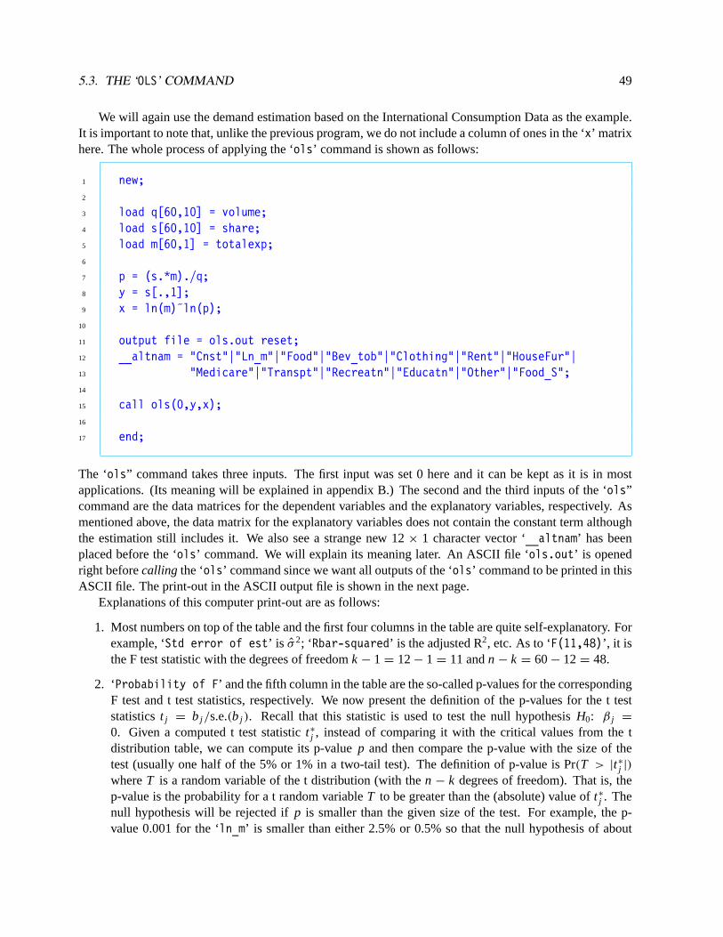
5.3. THE ‘OLS’ COMMAND 49
We will again use the demand estimation based on the International Consumption Data as the example.It is important to note that, unlike the previous program, we do not include a column of ones in the ‘x’ matrixhere. The whole process of applying the ‘ols’ command is shown as follows:
1 new;2
3 load q[60,10] = volume;4 load s[60,10] = share;5 load m[60,1] = totalexp;6
7 p = (s.*m)./q;8 y = s[.,1];9 x = ln(m)˜ln(p);
10
11 output file = ols.out reset;12 __altnam = "Cnst"|"Ln_m"|"Food"|"Bev_tob"|"Clothing"|"Rent"|"HouseFur"|13 "Medicare"|"Transpt"|"Recreatn"|"Educatn"|"Other"|"Food_S";14
15 call ols(0,y,x);16
17 end;
The ‘ols” command takes three inputs. The first input was set 0 here and it can be kept as it is in mostapplications. (Its meaning will be explained in appendix B.) The second and the third inputs of the ‘ols”command are the data matrices for the dependent variables and the explanatory variables, respectively. Asmentioned above, the data matrix for the explanatory variables does not contain the constant term althoughthe estimation still includes it. We also see a strange new 12× 1 character vector ‘__altnam’ has beenplaced before the ‘ols’ command. We will explain its meaning later. An ASCII file ‘ols.out’ is openedright beforecalling the ‘ols’ command since we want all outputs of the ‘ols’ command to be printed in thisASCII file. The print-out in the ASCII output file is shown in the next page.
Explanations of this computer print-out are as follows:
1. Most numbers on top of the table and the first four columns in the table are quite self-explanatory. Forexample, ‘Std error of est’ is σ 2; ‘Rbar-squared’ is the adjusted R2, etc. As to ‘F(11,48)’, it isthe F test statistic with the degrees of freedomk − 1 = 12− 1 = 11 andn − k = 60− 12 = 48.
2. ‘Probability of F’ and the fifth column in the table are the so-called p-values for the correspondingF test and t test statistics, respectively. We now present the definition of the p-values for the t teststatisticst j = b j /s.e.(b j ). Recall that this statistic is used to test the null hypothesisH0: β j =
0. Given a computed t test statistict∗
j , instead of comparing it with the critical values from the tdistribution table, we can compute its p-valuep and then compare the p-value with the size of thetest (usually one half of the 5% or 1% in a two-tail test). The definition of p-value is Pr(T > |t∗
j |)
whereT is a random variable of the t distribution (with then − k degrees of freedom). That is, thep-value is the probability for a t random variableT to be greater than the (absolute) value oft∗
j . Thenull hypothesis will be rejected ifp is smaller than the given size of the test. For example, the p-value 0.001 for the ‘ln_m’ is smaller than either 2.5% or 0.5% so that the null hypothesis of about

50 CHAPTER 5. GAUSS PROGRAM FOR LINEAR REGRESSION
1 Valid cases: 60 Dependent variable: Food_S2 Missing cases: 0 Deletion method: None3 Total SS: 10706.924 Degrees of freedom: 484 R-squared: 0.766 Rbar-squared: 0.7125 Residual SS: 2505.546 Std error of est: 7.2256 F(11,48): 14.283 Probability of F: 0.0007
8 Standard Prob Standardized Cor with9 Variable Estimate Error t-value >|t| Estimate Dep Var
10 -----------------------------------------------------------------------------11 Cnst 50.848501 10.763414 4.724198 0.000 --- ---12 Ln_m -8.797151 2.566394 -3.427826 0.001 -1.626372 -0.29204513 Food 1.686658 5.044760 0.334339 0.740 0.277730 0.07597114 Bev_tob 5.236882 3.612661 1.449591 0.154 0.828485 0.17312915 Clothing 1.507999 3.872228 0.389440 0.699 0.251680 0.06041116 Rent 0.926101 2.551713 0.362933 0.718 0.153014 0.08770217 HouseFur 4.350814 3.660329 1.188640 0.240 0.738807 0.01416218 Medicare -1.606652 3.176194 -0.505842 0.615 -0.276045 0.00208919 Transpt -4.483241 3.197497 -1.402110 0.167 -0.745650 0.06992220 Recreatn 6.517217 3.680082 1.770943 0.083 1.075507 0.07865921 Educatn -3.036182 3.312132 -0.916685 0.364 -0.533106 -0.14405622 Other -1.396618 4.391565 -0.318023 0.752 -0.224140 0.094973

5.3. THE ‘OLS’ COMMAND 51
the regression coefficient for the log income will be rejected in a two-tail test (i.e., the effect of logincome is significant). The definition and the use of the p-value for the F test are similar.
There are a number of GAUSS commands which can also be used to evaluate the p-values for thevarious test statistic with different distributions. For example, to evaluate the p-values of an F teststatistic 14.283 computed from the previous program, we use
1 p_value = cdffc(14.283,11,48);
In this ‘cdffc’ command, the first input is the computed F-test statistic, the second and the third inputsare the two degrees of freedom. The more precise definition of the ‘cdffc’ command is that it givesone minus the value of the cumulative F distribution function at 14.283. Other than F-distribution, wehave the following GAUSS command for other distributions:
1 p = cdfnc(z); /* For the normal distribution. */2 p = cdftc(t,df); /* For the t distribution. The second input is3 the degree of freedom. */4 p = cdfchic(t,df); /* For the chi-square distribution. The second5 input is the degree of freedom. */
Obviously, if we apply the ‘cdftc’ command to the absolute value of the t-ratio for log income: -3.427826: i.e., ‘cdftc(3.427876,48)’, the resulting p-value should be 0.001, as shown in the fifthcolumn of the above table.
3. The numbers in the last two columns of the table are two new statistics we haven’t considered yet. Thelast column gives the estimated correlation coefficient between the dependent variableYi and each ofthe explanatory variablesX j i , which is defined as∑n
i =1(Yj i − Yj )(X j i − X j )√∑ni =1(Yi − Y)2·
∑ni =1(X j i − X j )2
.
Given the OLS estimateb j for the j -th regression coefficient, the standardized estimate in the sixthcolumn is defined by
b j
√∑ni =1(X j i − X j )2∑n
i =1(Yi − Y)2.
4. The above tabulated estimation results are not the only output from the ‘ols’ procedure. In fact,eleven additional output matrices are also produced. They are suppressed in the above examples, butcan be retrieved if we type
1 {vnam,mmt,b,stb,vb,seb,s2,cor,r2,e,d} = ols(0,y,x);

52 CHAPTER 5. GAUSS PROGRAM FOR LINEAR REGRESSION
Here in front of the ‘ols’ command we have 11 matrix names enclosed in braces and an equality sign.Besides the printed results in the output ASCII file, those 11 output matrices are also the computationoutputs of the ‘ols’ command.
Among the 11 output matrices the following seven are something we are familiar with: ‘b’ (the OLSestimateb), ‘vb’ (the estimated variance-covariance matrix ofb), ‘seb’ (the standard errors ofb), ‘s2’(σ 2), ‘r2’ (R2), ‘e’ (the residuale = y−Xb), and ‘d’ (the Durbin-Watson statistic). The output vector‘stb’ contains the standardized OLS estimates for those non-constant explanatory variables which hasjust been defined above. The output vector ‘vnam’ contains the variable names, including those for theconstant term (the first element) and the dependent variable (the last element). The matrix ‘mmt’ givesthe cross-product (i.e., [X y ]′[ X y ]) and ‘cor’ contains the correlation coefficient matrix for thenon-constant explanatory variables and the dependent variable (which is included as the last variable).In general the residual vector ‘e’ and the scalar ‘d’ for the Durbin-Watson statistic are 0 unless wereset theswitch ‘_olsres’ from its default value 0 to 1 before executing the ‘ols’ command. Theexplanation ofswitchwill be given below.
Besides the print-out in the output ASCII file, why do we need those 11 output matrices? The reasonis that we may use those matrices for additional computation. For example, the residual vector ‘e’may be used to compute additional test statistics. This computation can proceed directly after the‘ols’ command in the same program.
5. We now go back to the explanation of the new expression ‘__altnam’ in the program. The ‘ols”command offers sixswitches(their formal names areglobal variableswhich will be discussed morefully in section 8.2) with which we can control some aspects of the OLS estimation. These switchesare simply matrix variables whose values are to be set by us. The ‘ols” command will check thevalues of these switches before implementing its calculation. These switches all have default valueswhich can usually be left as they are. Nevertheless, we can easily change those aspects of the ‘ols’command that are controlled by the switches by assigning different values to the switches. Here, wewill discuss three switches only: the matrix variables ‘__con’, ‘ __altnam’, and ‘_olsres’. Note thatthe names of the first two variables are prefixed with two underlines. This unique form distinguishesthem from other variable names. Let’s now consider the meanings of these two switches:
(1) The switch ‘__con’:If we do not want to include the constant term in the OLS estimation, then we should set theswitch ‘__con’ to 0 before calling the ‘ols’ procedure. The default value of ‘__con’ is 1, withwhich the constant term will be included in the OLS estimation. In the above program theredefinition of the switch ‘__con’ is not included, so the estimation will include the constantterm (even if the data matrix ‘x’ does not contain a column for the constant term.)
(2) The switch ‘__altnam’:If we want to give specific names to the explanatory variables and the dependent variable, weneed to assign a character vector of names to the switch ‘__altnam’, where the first one shouldalways be the name for the constant term if it is included and the last one should be the namefor the dependent variable. This is exactly how we did in the above program. So the namefor the constant term is ‘Cnst’, the name for the log income variable is ‘Ln_m’, etc. The namefor the dependent variable, specified as the last character, is ‘Food_S’. Note that the size of the‘__altnam’ vector is 13× 1. If the switch ‘__altnam’ is not included in the program, then thedefault names for the explanatory variables are ‘CONSTANT’, ‘ X1’, ‘ X2’, ‘ X3’, . . .
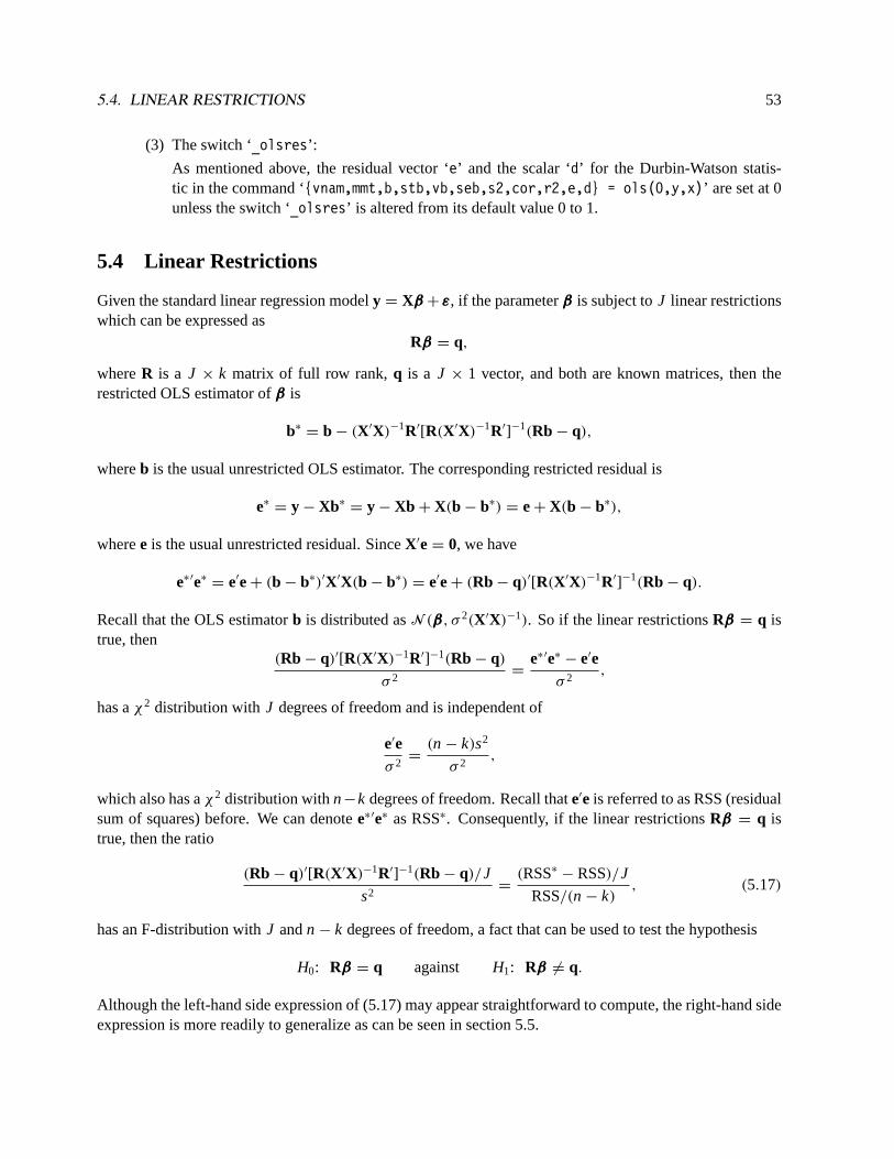
5.4. LINEAR RESTRICTIONS 53
(3) The switch ‘_olsres’:
As mentioned above, the residual vector ‘e’ and the scalar ‘d’ for the Durbin-Watson statis-tic in the command ‘{vnam,mmt,b,stb,vb,seb,s2,cor,r2,e,d} = ols(0,y,x)’ are set at 0unless the switch ‘_olsres’ is altered from its default value 0 to 1.
5.4 Linear Restrictions
Given the standard linear regression modely = Xβββ+ εεε, if the parameterβββ is subject toJ linear restrictionswhich can be expressed as
Rβββ = q,
whereR is a J × k matrix of full row rank,q is a J × 1 vector, and both are known matrices, then therestricted OLS estimator ofβββ is
b∗= b − (X′X)−1R′[R(X′X)−1R′]−1(Rb − q),
whereb is the usual unrestricted OLS estimator. The corresponding restricted residual is
e∗= y − Xb∗
= y − Xb + X(b − b∗) = e+ X(b − b∗),
wheree is the usual unrestricted residual. SinceX′e = 0, we have
e∗′e∗= e′e+ (b − b∗)′X′X(b − b∗) = e′e+ (Rb − q)′[R(X′X)−1R′]−1(Rb − q).
Recall that the OLS estimatorb is distributed asN (βββ, σ 2(X′X)−1). So if the linear restrictionsRβββ = q istrue, then
(Rb − q)′[R(X′X)−1R′]−1(Rb − q)σ 2
=e∗′e∗
− e′eσ 2
,
has aχ2 distribution withJ degrees of freedom and is independent of
e′eσ 2
=(n − k)s2
σ 2,
which also has aχ2 distribution withn−k degrees of freedom. Recall thate′e is referred to as RSS (residualsum of squares) before. We can denotee∗′e∗ as RSS∗. Consequently, if the linear restrictionsRβββ = q istrue, then the ratio
(Rb − q)′[R(X′X)−1R′]−1(Rb − q)/J
s2=(RSS∗
− RSS)/J
RSS/(n − k), (5.17)
has an F-distribution withJ andn − k degrees of freedom, a fact that can be used to test the hypothesis
H0: Rβββ = q against H1: Rβββ 6= q.
Although the left-hand side expression of (5.17) may appear straightforward to compute, the right-hand sideexpression is more readily to generalize as can be seen in section 5.5.

54 CHAPTER 5. GAUSS PROGRAM FOR LINEAR REGRESSION
An Example The difference between an Engel curve model (5.15) and a demand model (5.16) is that thelatter includes prices. Which of the two models is more suitable for the International Consumption Datadepends on how important the price effects are. The F test is needed to decide whether the price effects arejointly significant. To conduct such a test, we start with the demand model which can be represented by thegeneral notationy = Xβββ + εεε, with X including a constant term, log income, and ten log prices. Among thetwelve elements ofβββ, what we try to decide is whether the last ten (the coefficients for the log prices) areequal to zero or not. In other words, the hypothesis is whether the ten price coefficients are equal to zeroor not. Formally, this null hypothesis can be expressed as a set of ten linear restrictions on the regressioncoefficient vectorβββ as follows:
Rβββ =
0 0 1 0 0 · · · 0
0 0 0 1 0 · · · 0
0 0 0 0 1 · · · 0...
......
......
. . ....
0 0 0 0 0 · · · 1
β1
β2
β3
...
β12
= [ 0 0 I10 ] ·βββ =
β3
β4
β5
...
β12
= 0.
whereI10 is a 10× 10 identity matrix and0 is a 10× 1 vector of zeros. Given this setup, then it is fairlystraightforward to write a program to test the significance of the price effects:
1 new;2
3 load q[60,10] = volume;4 load s[60,10] = share;5 load m[60,1] = totalexp;6
7 p = (m.*s)./q;8
9 y = s[.,1];10 x = ones(60,1)˜ln(m˜p);11 n = rows(y);12 k = cols(y);13
14 e = y - x*invpd(x’x)*x’y;15 s2 = e’e/(n-k);16 r = zeros(10,2)˜eye(10);17 f = (r*b)’invpd(r*invpd(x’x)*r’)*r*b/(10*s2);18 pv = cdffc(f,10,n-k);19
20 output file = test.out on;21 format /rd 8,4;22 " The F test statistic is " f;;" with a p-value " pv;23
24 end;
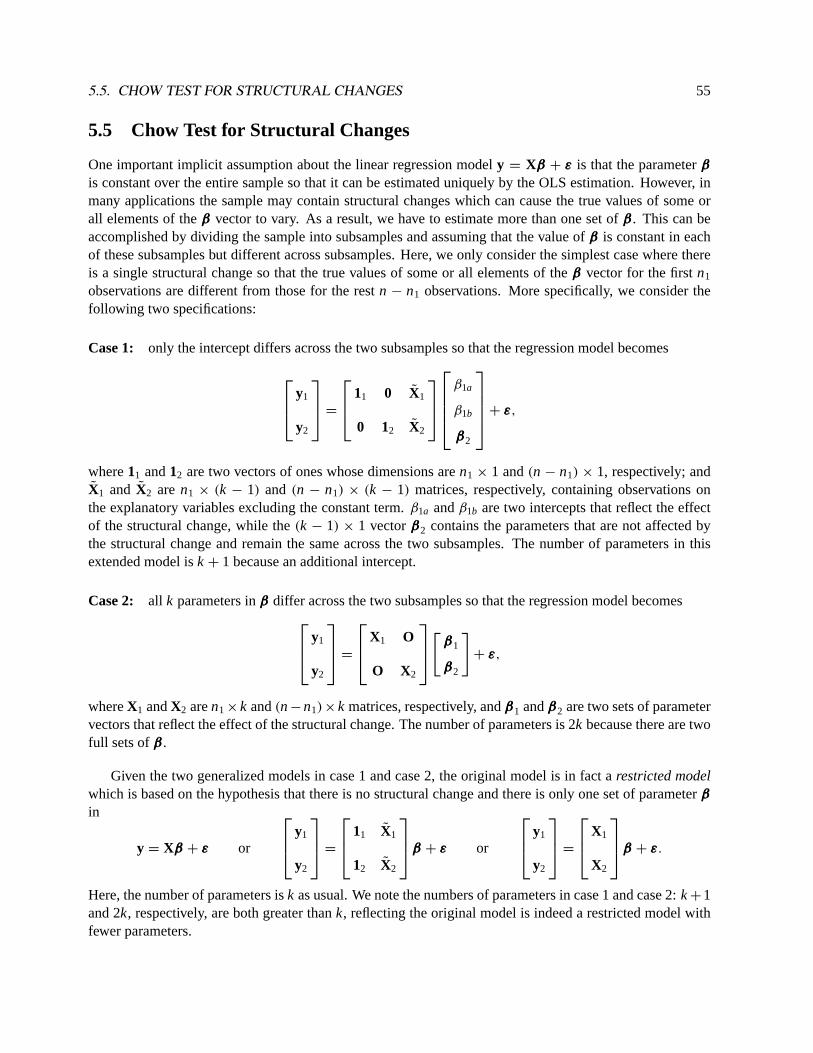
5.5. CHOW TEST FOR STRUCTURAL CHANGES 55
5.5 Chow Test for Structural Changes
One important implicit assumption about the linear regression modely = Xβββ + εεε is that the parameterβββis constant over the entire sample so that it can be estimated uniquely by the OLS estimation. However, inmany applications the sample may contain structural changes which can cause the true values of some orall elements of theβββ vector to vary. As a result, we have to estimate more than one set ofβββ. This can beaccomplished by dividing the sample into subsamples and assuming that the value ofβββ is constant in eachof these subsamples but different across subsamples. Here, we only consider the simplest case where thereis a single structural change so that the true values of some or all elements of theβββ vector for the firstn1
observations are different from those for the restn − n1 observations. More specifically, we consider thefollowing two specifications:
Case 1: only the intercept differs across the two subsamples so that the regression model becomes
y1
y2
=
11 0 X1
0 12 X2
β1a
β1b
βββ2
+ εεε,
where11 and12 are two vectors of ones whose dimensions aren1 × 1 and(n − n1) × 1, respectively; andX1 and X2 are n1 × (k − 1) and (n − n1) × (k − 1) matrices, respectively, containing observations onthe explanatory variables excluding the constant term.β1a andβ1b are two intercepts that reflect the effectof the structural change, while the(k − 1) × 1 vectorβββ2 contains the parameters that are not affected bythe structural change and remain the same across the two subsamples. The number of parameters in thisextended model isk + 1 because an additional intercept.
Case 2: all k parameters inβββ differ across the two subsamples so that the regression model becomes y1
y2
=
X1 O
O X2
[βββ1
βββ2
]+ εεε,
whereX1 andX2 aren1 ×k and(n−n1)×k matrices, respectively, andβββ1 andβββ2 are two sets of parametervectors that reflect the effect of the structural change. The number of parameters is 2k because there are twofull sets ofβββ.
Given the two generalized models in case 1 and case 2, the original model is in fact arestricted modelwhich is based on the hypothesis that there is no structural change and there is only one set of parameterβββ
in
y = Xβββ + εεε or
y1
y2
=
11 X1
12 X2
βββ + εεε or
y1
y2
=
X1
X2
βββ + εεε.
Here, the number of parameters isk as usual. We note the numbers of parameters in case 1 and case 2:k+1and 2k, respectively, are both greater thank, reflecting the original model is indeed a restricted model withfewer parameters.

56 CHAPTER 5. GAUSS PROGRAM FOR LINEAR REGRESSION
We can fit the model of no structural change, as opposed to case 1 and case 2 structural changes, into theframework of the general linear restrictions. Given the case 1 structural change, theunrestrictedparametervector containsβ1a, β1b, andβββ2, while theR matrix corresponding to the restricted model of no structuralchange is a 1× (k + 1) vector [1−1 0′], where0 is ak × 1 vector of zeros. So the restrictionRβββ = q canbe written as
[1 −1 0′
]β1a
β1b
βββ2
= 0.
Similarly, in case 2 the restricted model of no structural change imposes the following restriction on theparameter vector: [
I k −I k
] [βββ1
βββ2
]= 0,
whereI k is ak × k identity matrix.The above expressions of theR matrix can be used to formulate statistics for testing the null hypothesis
of no structural change against the alternative hypothesis of case 1 and case 2, respectively. However, aneasier way to construct the test statistics is based on residuals and the corresponding RSS from each of thethree models. Let RSS be the residual sum of squares from the restricted model (i.e., the original model)and RSS1 and RSS2 from the case 1 model and the case 2 model, respectively.
1. The F-test statistic against case 1 structural change is
F1 =(RSS− RSS1)/1
RSS1/(n − k − 1),
with degrees of freedom 1 andn − k − 1.
2. The F-test statistic against case 2 structural change is
F2 =(RSS− RSS2)/k
RSS2/(n − 2k),
with degrees of freedomk andn − 2k.
3. Finally, we note case 1 is in fact a special case of case 2. So we can test case 1 against case 2 usingthe following test statistic:
F =(RSS1 − RSS2)/(k − 1)
RSS2/(n − 2k).
The degrees of freedom arek − 1 andn − 2k.
These F-tests, particularlyF2, are usually referred to as the Chow test. The GAUSS program for Chowtests is quite straightforward. What needs to be done is simply the calculation of three types of residuals andthe corresponding RSS, as well as the degrees of freedom. From equations (5.2) and (5.9) we know RSS isdefined by
RSS= e′e = (y − Xb)′(y − Xb) = y′y − y′X(X′X)−1X′y.

5.5. CHOW TEST FOR STRUCTURAL CHANGES 57
Also, each RSS is associated with a particular degree of freedom, which is equal to the sample size (i.e., therow number of theX matrix) minus the number of parameters (i.e., the column number of theX matrix).Furthermore, by a closer inspection of each of the Chow test statistics, we find that the denominator isan RSS divided by its associated degree of freedom, while the numerator is the difference between twoRSS’s, divided by the difference between the two associated degrees of freedom. This general pattern helpssimplifying the GAUSS program.
Given then × k matrix of the explanatory variables ‘x’ from the original model (i.e., the restrictedmodel), in which the first ‘n1’ observations belong to the first subsample and the rest ‘n - n1’ observationsbelong to the second subsample, we have to carefully organize then × (k + 1) andn × 2k matrices ‘x1’ and‘x2’ for the two unrestricted models – case 1 and case 2, respectively. Once the three matrices of explanatoryvariables for the three models are defined, then we can use the same formulas to compute the RSS and theassociated degrees of freedom for the three models, followed by the corresponding Chow test statistics, ‘f1’,“f2’, and ‘f’. The p-values of these test statistics can also be computed easily.
1 /* The expanded matrix of explanatory variables for the case 1 model. */2 x1 = (ones(n1,1)˜zeros(n1,1)˜x[1:n1,2:k])|3 (zeros(n-n1,1)˜ones(n-n1,1)˜x[(n1+1):n,2:k]);4
5 /* The expanded matrix of explanatory variables for the case 2 model. */6 x2 = (x[1:n1,.]˜zeros(n1,k))|(zeros(n-n1,k)˜x[(n1+1):n,.]);7
8 rss = y’y - y’x*invpd(x’x)*x’y; /* RSS from the restricted model. */9 df = rows(x) - cols(x); /* The degree of freedom of ‘rss’. */
10
11 rss1 = y’y - y’x1*invpd(x1’x1)*x1’y; /* RSS from the case 1 model. */12 df1 = rows(x1) - cols(x1); /* The degree of freedom of ‘rss1’. */13
14 /* The F test statistic for testing case 1 against the restricted model. */15 f1 = ((rss - rss1)/(df1 - df)/(rss1/df1);16 /* The p-value of the test statistic. */17 pv1 = cdffc(f1,df1-df,df1);18
19 rss2 = y’y - y’x2*invpd(x2’x2)*x2’y; /* RSS from the case 2 model. */20 df2 = rows(x2) - cols(x2); /* The degree of freedom of ‘rss2’. */21 f2 = ((rss - rss2)/(df2 - df)/(rss2/df2);22 pv2 = cdffc(f2,df2-df,df2);23
24 /* The F test statistic for testing case 2 against case 1. */25 f = ((rss1 - rss2)/(df2 - df1)/(rss2/df2);26 pv = cdffc(f,df2-df1,df2);
Recall that the null hypothesis will be rejected if the p-value is smaller than the designated size (usually5% or 1%). The most interesting feature of the above program is the similarity among the three sets ofcommands for computing the three test statistics.

58 CHAPTER 5. GAUSS PROGRAM FOR LINEAR REGRESSION

Chapter 6Relational Operators and Logic Operators
Other than the usual arithmetic operators, there are relational and logic operators in GAUSS which produceresults that can have only two values: either “true” (recorded as the number 1) or “false” (recorded as thenumber 0).
6.1 Relational Operators
In GAUSS there are six relational operators. Each of these relational operators has two equivalent notation:
1. ‘<’ (or ‘ lt’), which means “smaller than”.
2. ‘<=’ (or ‘ le’), which means “smaller than or equal to”.
3. ‘==’ (or ‘ eq’), which means “equal to”.
4. ‘/=’ (or ‘ ne’), which means “not equal to”.
5. ‘>’ (or ‘ gt’), which means “greater than”.
6. ‘>=’ (or ‘ ge’), which means “greater than or equal to”.
Consider the example:
1 a = (x /= y);
If ‘ x’ and ‘y’ are two scalar variables with different values, then the right-hand side relational operation willbe true and the value of ‘a’ will be ‘ 1’. If ‘ x’ and ‘y’ have the same values, then the result on the right-handside relational operation is false and the value of ‘a’ will be ‘ 0’. Note that the relational operator for “equalto” consists of two equal signs ‘==’, which is very different in meaning from the single equal sign ‘=’.
If the relational operators are preceded by a dot ‘.’ then they become element-by-element operators. Forexample, if ‘x’ and ‘y’ are twon × 1 vectors and
1 a = (x ./= y);
then ‘a’ will be an n × 1 vector of 0 and 1, representing the results ofn relational operations between then corresponding elements of ‘x’ and ‘y’. Also, if the dimensions of ‘x’ and ‘y’ are not the same, then theusual rule for element-by-element operations will apply.
The relational operators, particularly ‘==’ and ‘/=’, can also be applied to character vectors or stringswith each operator preceded by ‘$’. For example,
59

60 CHAPTER 6. RELATIONAL OPERATORS AND LOGIC OPERATORS
1 a = ("old" $/= "young");2 b = (region .$== "SOUTH");
The value of ‘a’ is 1 since the relation on the right-hand side is always true. The dimension of ‘b’ will bethe same as that of the character vector ‘region’. Whether the value of an element of ‘b’ is 1 or 0 dependson whether the corresponding element in ‘region’ contains characters ‘SOUTH’ or not.
6.2 Logic Operators
There are five logic operators in GAUSS: ‘and’, ‘ or’, ‘ not’, ‘ xor’, and ‘eqv’. Among them the first threeare used most often.
1 a = (x and y);2 b = (x or y);3 c = not x;4 e = (x eqv y);5 f = (x xor y);
Here, the values in both scalars ‘x’ and ‘y’ must be either 0 and 1; that is, they themselves may be thetrue/false results of some relational or logical operations. The value of ‘a’ is 1 when both ‘x’ and ‘y’ are 1;‘a’ is 0 for all other cases. The value of ‘b’ is 0 when both ‘x’ and ‘y’ are 0; ‘b’ is 1 for all other cases. Thevalue of ‘c’ is just opposite to that of ‘x’: if ‘ x’ is 1, then ‘c’ is 0; and vice versa. The value of ‘e’ is 1 when‘x’ and ‘y’ are both 1 or both 0. The value of ‘f’ is 1 when ‘x’ and ‘y’ have opposite values. The logicaloperators can also be made as element-by-element operators if they are preceded by a dot ‘.’ So ‘.and’,‘.or’, ‘ .not’, ‘ .eqv’, and ‘.xor’ are all element-by-element logical operators.
6.3 Conditional Statements
The true/false results of relational or logic operations are usually used as conditions for determining whetherto execute a set of commands through the following design:
1 if (true/false statement A);2 expressions I;3 endif;4 expressions II;
If the ‘true/false statement A’ is true, then ‘expressions I’ will be executed, followed by‘expressions II’ after the ‘endif’ expression. If the ‘true/false statement A’ is false, then‘expressions I’ will be skipped and only ‘expressions II’ will be executed. Each ‘if’ command mustbe paired with an ‘endif’ command. Here is a simple example:
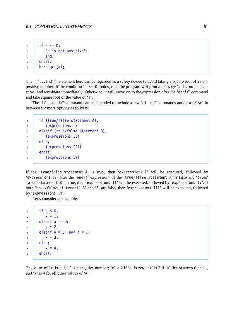
6.3. CONDITIONAL STATEMENTS 61
1 if a <= 0;2 "a is not positive";3 end;4 endif;5 b = sqrt(a);
The ‘if...endif’ statement here can be regarded as a safety device to avoid taking a square root of a non-positive number. If the condition ‘a <= 0’ holds, then the program will print a message ‘a is not posi-tive’ and terminate immediately. Otherwise, it will move on to the expression after the ‘endif’ commandand take square root of the value of ‘a’.
The ‘if...endif’ command can be extended to include a few ‘elseif’ commands and/or a ‘else’ inbetween for more options as follows:
1 if (true/false statement A);2 (expressions I)3 elseif (true/false statement B);4 (expressions II)5 else;6 (expressions III)7 endif;8 (expressions IV)
If the ‘true/false statement A’ is true, then ‘expressions I’ will be executed, followed by‘expressions IV’ after the ‘endif’ expression. If the ‘true/false statement A’ is false and ‘true/false statement B’ is true, then ‘expressions II’ will be executed, followed by ‘expressions IV’. Ifboth ‘true/false statement’ ‘ A’ and ‘B’ are false, then ‘expressions III’ will be executed, followedby ‘expressions IV’.
Let’s consider an example:
1 if a < 0;2 x = 1;3 elseif a == 0;4 x = 2;5 elseif a > 0 .and a < 1;6 x = 3;7 else;8 x = 4;9 endif;
The value of ‘x’ is 1 if ‘ a’ is a negative number; ‘x’ is 2 if ‘ a’ is zero; ‘x’ is 3 if ‘ a’ lies between 0 and 1,and ‘x’ is 4 for all other values of ‘a’.

62 CHAPTER 6. RELATIONAL OPERATORS AND LOGIC OPERATORS
6.4 Row-Selectors: the ‘selif’ and ‘ delif’ Commands
A useful technique for data rearrangement is to select rows (observations) from a data matrix based on thevalues of the corresponding elements of a column vector. For example, given the 60×10 matrix ‘s’ of budgetshare data on 10 commodities for 60 countries, we want to select those observations with the Food budgetshare (the first column) lying between 0.3 and 0.8. In other words, the process of selecting observations isbased on a relational operation on the single variable – the Food budget share. Situations like this can beeasily handled using the powerful ‘selif’ or ‘ delif’ commands:
1 e = (s[.,1] .>= 0.3 .and s[.,1] .<= 0.8);2 s1 = selif(s,e);
Here, ‘e’ is a 60× 1 vector of 1 and 0, representing the results of element-by-element relational operations.The ‘selif’ command will pick those rows of the ‘s’ matrix which correspond to all the “1” in the ‘e’vector, delete those rows of the ‘s’ matrix which correspond to all the “0” in the ‘e’ vector, and then form asmaller matrix ‘s1’. A similar command is
1 f = (s[.,1] .< 0.3 .or s[.,1] .> 0.8);2 s2 = delif(s,f);
where ‘f’ is again a 60× 1 vector of 1 and 0, representing the results of element-by-element relationaloperations which are exactly opposite to the ‘e’ vector before. The ‘delif’ command will delete those rowsof the ‘s’ matrix which correspond to all the “1” in the ‘e’ vector, and then form the resulting ‘s2’ matrix.Obviously, the two resulting matrices ‘s1’ and ‘s2’ are identical.
The two arguments of the ‘selif’ and ‘delif’ commands should have the same row number while thesecond argument must be a column vector of 0 and 1, which usually are the results of element-by-elementrelational operations.
6.5 Dummy Variables in Linear Regression Models
In this section we will first review how dummy variables work in a simple linear regression model:
yi = α + βxi + εi ,
we then suggest how dummy variables can be constructed in GAUSS. We will find that the element-by-element relational operators and logical operators are very useful in generating dummy variables.
6.5.1 Binary Dummy Variables
A dummy variable, say,di , is used to characterize two mutually exclusive categories. Based on which ofthe two categories an observationi belongs to, we assign a value, either 0 or 1, to the dummy variabledi . Including a dummy variable in a linear regression model allows us to examine how the differencebetween the two categories may affect the dependent variable. For example, the sampled countries of theInternational Consumption Data can be divided into two categories: North American/European and the
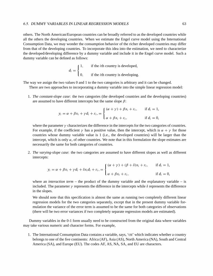
6.5. DUMMY VARIABLES IN LINEAR REGRESSION MODELS 63
others. The North American/European countries can be broadly referred to as the developed countries whileall the others the developing countries. When we estimate the Engel curve model using the InternationalConsumption Data, we may wonder the consumption behavior of the richer developed countries may differfrom that of the developing countries. To incorporate this idea into the estimation, we need to characterizethe developed/developing difference by a dummy variable and include it in the Engel curve model. Such adummy variable can be defined as follows:
di =
{1, if the i th country is developed,
0, if the i th country is developing.
The way we assign the two values 0 and 1 to the two categories is arbitrary and it can be changed.There are two approaches to incorporating a dummy variable into the simple linear regression model:
1. The constant-slope case: the two categories (the developed countries and the developing countries)are assumed to have different intercepts but the same slopeβ:
yi = α + βxi + γdi + εi ,=
{(α + γ )+ βxi + εi , if di = 1,
α + βxi + εi , if di = 0,
where the parameterγ characterizes the difference in the intercepts for the two categories of countries.For example, if the coefficientγ has a positive value, then the intercept, which isα + γ for thosecountries whose dummy variable value is 1 (i.e., the developed countries) will be larger than theintercept, which is onlyα, of other countries. We note that in this formulation the slope estimates arenecessarily the same for both categories of countries.
2. The varying-slope case: the two categories are assumed to have different slopes as well as differentintercepts:
yi = α + βxi + γdi + δxi di + εi ,=
{(α + γ )+ (β + δ)xi + εi , if di = 1,
α + βxi + εi , if di = 0,
where aninteraction term– the product of the dummy variable and the explanatory variable – isincluded. The parameterγ represents the difference in the intercepts whileδ represents the differencein the slopes.
We should note that this specification is almost the same as running two completely different linearregression models for the two categories separately, except that in the present dummy variable for-mulation the variance of the error term is assumed to be the same for both categories of observations(there will be two error variances if two completely separate regression models are estimated).
Dummy variables in the 0-1 form usually need to be constructed from the original data where variablesmay take various numeric and character forms. For example,
1. The International Consumption Data contains a variable, says, ‘ctt’ which indicates whether a countrybelongs to one of the five continents: Africa (AF), Asia (AS), North America (NA), South and CentralAmerica (SA), and Europe (EU). The codes AF, AS, NA, SA, and EU are characters.
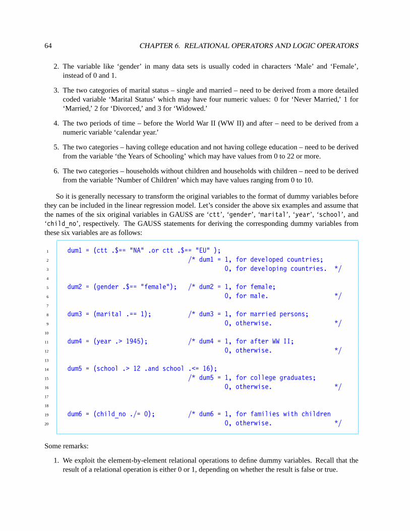
64 CHAPTER 6. RELATIONAL OPERATORS AND LOGIC OPERATORS
2. The variable like ‘gender’ in many data sets is usually coded in characters ‘Male’ and ‘Female’,instead of 0 and 1.
3. The two categories of marital status – single and married – need to be derived from a more detailedcoded variable ‘Marital Status’ which may have four numeric values: 0 for ‘Never Married,’ 1 for‘Married,’ 2 for ‘Divorced,’ and 3 for ‘Widowed.’
4. The two periods of time – before the World War II (WW II) and after – need to be derived from anumeric variable ‘calendar year.’
5. The two categories – having college education and not having college education – need to be derivedfrom the variable ‘the Years of Schooling’ which may have values from 0 to 22 or more.
6. The two categories – households without children and households with children – need to be derivedfrom the variable ‘Number of Children’ which may have values ranging from 0 to 10.
So it is generally necessary to transform the original variables to the format of dummy variables beforethey can be included in the linear regression model. Let’s consider the above six examples and assume thatthe names of the six original variables in GAUSS are ‘ctt’, ‘ gender’, ‘ marital’, ‘ year’, ‘ school’, and‘child_no’, respectively. The GAUSS statements for deriving the corresponding dummy variables fromthese six variables are as follows:
1 dum1 = (ctt .$== "NA" .or ctt .$== "EU" );2 /* dum1 = 1, for developed countries;3 0, for developing countries. */4
5 dum2 = (gender .$== "female"); /* dum2 = 1, for female;6 0, for male. */7
8 dum3 = (marital .== 1); /* dum3 = 1, for married persons;9 0, otherwise. */
10
11 dum4 = (year .> 1945); /* dum4 = 1, for after WW II;12 0, otherwise. */13
14 dum5 = (school .> 12 .and school .<= 16);15 /* dum5 = 1, for college graduates;16 0, otherwise. */17
18
19 dum6 = (child_no ./= 0); /* dum6 = 1, for families with children20 0, otherwise. */
Some remarks:
1. We exploit the element-by-element relational operations to define dummy variables. Recall that theresult of a relational operation is either 0 or 1, depending on whether the result is false or true.
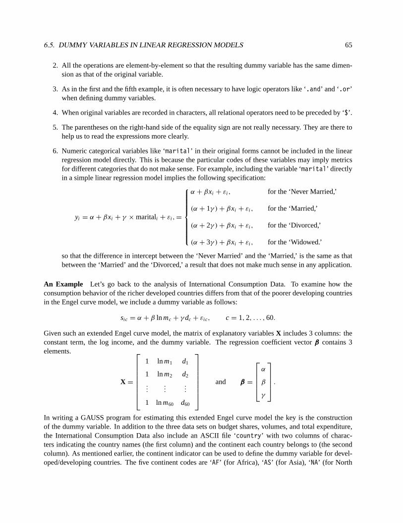
6.5. DUMMY VARIABLES IN LINEAR REGRESSION MODELS 65
2. All the operations are element-by-element so that the resulting dummy variable has the same dimen-sion as that of the original variable.
3. As in the first and the fifth example, it is often necessary to have logic operators like ‘.and’ and ‘.or’when defining dummy variables.
4. When original variables are recorded in characters, all relational operators need to be preceded by ‘$’.
5. The parentheses on the right-hand side of the equality sign are not really necessary. They are there tohelp us to read the expressions more clearly.
6. Numeric categorical variables like ‘marital’ in their original forms cannot be included in the linearregression model directly. This is because the particular codes of these variables may imply metricsfor different categories that do not make sense. For example, including the variable ‘marital’ directlyin a simple linear regression model implies the following specification:
yi = α + βxi + γ × maritali + εi ,=
α + βxi + εi , for the ‘Never Married,’
(α + 1γ )+ βxi + εi , for the ‘Married,’
(α + 2γ )+ βxi + εi , for the ‘Divorced,’
(α + 3γ )+ βxi + εi , for the ‘Widowed.’
so that the difference in intercept between the ‘Never Married’ and the ‘Married,’ is the same as thatbetween the ‘Married’ and the ‘Divorced,’ a result that does not make much sense in any application.
An Example Let’s go back to the analysis of International Consumption Data. To examine how theconsumption behavior of the richer developed countries differs from that of the poorer developing countriesin the Engel curve model, we include a dummy variable as follows:
sic = α + β ln mc + γdc + εic, c = 1,2, . . . ,60.
Given such an extended Engel curve model, the matrix of explanatory variablesX includes 3 columns: theconstant term, the log income, and the dummy variable. The regression coefficient vectorβββ contains 3elements.
X =
1 lnm1 d1
1 lnm2 d2
......
...
1 lnm60 d60
and βββ =
α
β
γ
.
In writing a GAUSS program for estimating this extended Engel curve model the key is the constructionof the dummy variable. In addition to the three data sets on budget shares, volumes, and total expenditure,the International Consumption Data also include an ASCII file ‘country’ with two columns of charac-ters indicating the country names (the first column) and the continent each country belongs to (the secondcolumn). As mentioned earlier, the continent indicator can be used to define the dummy variable for devel-oped/developing countries. The five continent codes are ‘AF’ (for Africa), ‘ AS’ (for Asia), ‘NA’ (for North
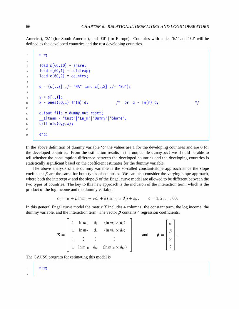
66 CHAPTER 6. RELATIONAL OPERATORS AND LOGIC OPERATORS
America), ‘SA’ (for South America), and ‘EU’ (for Europe). Countries with codes ‘NA’ and ‘EU’ will bedefined as the developed countries and the rest developing countries.
1 new;2
3 load s[60,10] = share;4 load m[60,1] = totalexp;5 load c[60,2] = country;6
7 d = (c[.,2] ./= "NA" .and c[.,2] ./= "EU");8
9 y = s[.,1];10 x = ones(60,1)˜ln(m)˜d; /* or x = ln(m)˜d; */11
12 output file = dummy.out reset;13 __altnam = "Cnst"|"Ln_m"|"Dummy"|"Share";14 call ols(0,y,x);15
16 end;
In the above definition of dummy variable ‘d’ the values are 1 for the developing countries and are 0 forthe developed countries. From the estimation results in the output filedummy.out we should be able totell whether the consumption difference between the developed countries and the developing countries isstatistically significant based on the coefficient estimates for the dummy variable.
The above analysis of the dummy variable is the so-called constant-slope approach since the slopecoefficientβ are the same for both types of countries. We can also consider the varying-slope approach,where both the interceptα and the slopeβ of the Engel curve model are allowed to be different between thetwo types of countries. The key to this new approach is the inclusion of the interaction term, which is theproduct of the log income and the dummy variable:
sic = α + β ln mc + γdc + δ (ln mc × dc)+ εic, c = 1,2, . . . ,60.
In this general Engel curve model the matrixX includes 4 columns: the constant term, the log income, thedummy variable, and the interaction term. The vectorβββ contains 4 regression coefficients.
X =
1 lnm1 d1 (ln m1 × d1)
1 lnm2 d2 (ln m2 × d2)
......
......
1 lnm60 d60 (ln m60 × d60)
and βββ =
α
β
γ
δ
.
The GAUSS program for estimating this model is
1 new;2

6.5. DUMMY VARIABLES IN LINEAR REGRESSION MODELS 67
3 load s[60,10] = share;4 load m[60,1] = totalexp;5 load c[60,2] = country;6
7 d = (c[.,2] ./= "NA" .and c[.,2] ./= "EU");8
9 y = s[.,1];10 x = ones(60,1)˜ln(m)˜d˜(ln(m).*d);11
12 output file = dummy.out on;13 __altnam = "Cnst"|"Ln_m"|"Dummy"|"Interact"|"Share";14 call ols(0,y,x);15
16 end;
Note that the construction of the interaction term ‘d.*ln(m)’ in the data matrix ‘x’ is quite easy because ofelement-by-element multiplication.
6.5.2 The Polychotomous Case
Variables like ‘ctt’ and ‘marital’ are referred to as polychotomous categorical variables because they havemore than two possible values. The way we have handled them is to construct dummy variables from them.However, information in these variables is usually more than what a single dummy variable can convey. Tofully reflect the information in a polychotomous categorical variable, we need to construct a set of dummyvariables. Furthermore, it is sometimes possible to derive a set of dummy variables from “continuous”variables like ‘year,’ ‘ school,’ and ‘child_no’.
Generalizing from the two approaches in the single dummy variable case, we have the following twoapproaches to including multiple dummy variables into a simple linear regression model:
1. The constant-slope case: It is very important to know that onlyJ −1 dummy variables are needed forthe J categories when the intercept term is included in the linear regression model. The specificationof the model is as follows:
yi = α + βxi +
J−1∑j =1
γ j d j i + εi ,
=
{(α + γ j )+ βxi + εi , if d j i = 1 anddki = 0, for all k 6= j , and j = 1, . . . , J − 1,
α + βxi + εi , if d j i = 0, for all j ,
where the category with alld j i = 0 is considered as thebase. γ j indicates the difference in theintercept between the base category and the category specified byd j i = 1 anddki = 0, for all k 6= j .
Consider the example of the four-category ‘marital’ variable. three dummy variables are needed tocarry all the information in ‘marital’ and they can be defined in GAUSS as follows:

68 CHAPTER 6. RELATIONAL OPERATORS AND LOGIC OPERATORS
1 m_dum1 = (marital .== 1);2 m_dum2 = (marital .== 2);3 m_dum3 = (marital .== 3);
Here, we note a variable ‘m_dum0’ which may be defined by ‘(marital .== 0)’ is deliberatelymissed because the category of the ‘Never Married’ is chosen as the base. For the ‘Never Married’ thevalues of the three dummy variables ‘m_dum1’, ‘ m_dum2’, and ‘m_dum3’ are all 0. As to the ‘Married,’the value of the dummy variable ‘m_dum1’ is 1 and the other two are 0. The specifications for othercategories are similar to that of the ‘Married.’
It is possible to use a single GAUSS statement to define ann × 3 matrix that includes all four dummyvariables ‘m_dum1’, ‘ m_dum2’, and ‘m_dum3’:
1 m_dum = (marital .== (1˜2˜3));
The resulting matrix ‘m_dum’ is equivalent to the horizontal concatenation of the four columns of‘m_dum1’, ‘ m_dum2’, and ‘m_dum3’ in the previous definition.
Let’s now consider another example of generating multiple dummy variables from thecontinuousvariable ‘school’. Suppose we want to create four dummy variables for the five categories: (1) somehigh school education; (2) high school graduates; (3) some college education; (4) college graduates;and (5) some postgraduate education; where the second category of high school graduates is taken asthe base. The GAUSS statements are
1 ed_dum1 = (school .<= 11);2 ed_dum3 = ((12 .< school) .and (school .<= 15));3 ed_dum4 = ((15 .< school) .and (school .<= 16));4 ed_dum5 = (16 .< school);
There seems no simple relational operations to create ann × 4 matrix that contains all four dummyvariables at one stroke. But there is a GAUSS command designed specifically for this purpose:
1 y = dummydn(x,e,j);
What this command does is following:
(1) Using elementse1, e2, . . ., of the second input ‘e’, which must be ak × 1 column of numbers inascending order, to partition the real line intok + 1 open-closed intervals:(−∞, e1], (e1, e2],. . . (ek−1, ek], (ek−1, ∞].
(2) Evaluating each element in the first input ‘x’, which is ann × 1 column, to determine which ofthe abovek + 1 open-closed intervals this element belongs to;

6.5. DUMMY VARIABLES IN LINEAR REGRESSION MODELS 69
(3) Creating ann × (k + 1) temporary matrix, say ‘z’, of dummy variables, each row contains a 1andk 0’s. Among thek + 1 element of thei -th row of ‘z’, which element is 1 depends on whichof the abovek + 1 open-closed intervals contains the value of thei -th element of ‘x’.
(4) The third input ‘j’, which must be an integer between 1 andk + 1, specifies the column to bedeleted from then × (k + 1) matrix ‘z’ in order to produce then × k output matrix ‘y’. Thedeleted column corresponds to the category that is designated as the base.
So in our example we should type
1 e = 11|12|15|16;2 ed_dum = dummydn(school,e,2);
The resultingn × 4 matrix ‘ed_dum’ is equivalent to the horizontal concatenation of the four columns‘ed_dum1’, ‘ ed_dum3’, ‘ ed_dum4’, and ‘ed_dum5’ in the earlier definition. Obviously, with the fourbreak points in the second input ‘e’ it is possible to create five categories from the input ‘school’,while the third input of the ‘dummydn’ command, which is 2 in our example, indicates which amongthe five categories is designated as the base so that the corresponding column will be deleted.
2. The varying-slope case: Again, J − 1 dummy variables are needed forJ categories and the modelbecomes
yi = α + βxi +
J−1∑j =1
γ j d j i +
J−1∑j =1
δ j xi d j i + εi ,
=
{(α + γ j )+ (β + δ j )xi + εi , if d j i = 1 anddki = 0, for all k 6= j , and j = 1, . . . , J − 1,
α + βxi + εi , if d j i = 0, for all j ,
where the category with alld j i = 0 is considered the base.γ j indicates the difference in the interceptandδ j indicates the difference in the slope between the base category and the category withd j i = 1anddki = 0, for all k 6= j .
In the previous example about the variable ‘school’ we have created ann × 4 matrix ‘ed_dum’ ofdummy variables. Now suppose we have a column of data ‘x0’ on the single continuous explanatoryvariablexi , then the new data matrix ‘x’ of all explanatory variables for the present varying-slope caseis formed by
1 x = ones(n,1)˜x0˜ed_dum˜(x0.*ed_dum);
The dimension of the matrix ‘x’ is n × 10.
As demonstrated by the example of generating multiple dummy variables from thecontinuousvariable‘school’, we note essentially any continuous variable can be transformed to a set of dummy variables.Doing so may be necessary in some applications because we are not always certain about whether the

70 CHAPTER 6. RELATIONAL OPERATORS AND LOGIC OPERATORS
regression coefficients of those continuous explanatory variables are constant over their entire ranges. In thenext subsection, we will explore another approach to the problem of non-constant regression coefficientswhich is based on another kind of categorization of the information from the continuous variables.
An Example Extending from the previous simple dummy variable analysis for the International Con-sumption data, we now study how the consumption behavior differs among the developed countries and thethree groups – the African, Asian, and South American countries – of the developing countries. That is, weare going to divide the 60 sampled countries into four categories. For four categories we need three dummyvariables, says,d1, d2, d3, whose exact definitions will depend on the choice of the base category. Here, wearbitrarily choose the developed countries as the base. The specific definitions of the dummy variables areas follows: For the developed countries the values of the three dummy variables are all zeros. The values ofd1, d2, andd3 for the African countries are 1, 0, and 0, respectively. For the Asian countries, the values are0, 1, and 0, respectively; and for the South American countries, the values are 0, 0, and 1, respectively.
We include the three dummy variables in the Engel curve model as follows:
sic = α + β ln mc + γ1d1c + γ2d2c + γ3d3c + εic, c = 1,2, . . . ,60.
In writing a GAUSS program for estimating this extended Engel curve model, the key is again the construc-tion of the dummy variable.
1 new;2
3 load s[60,10] = share;4 load m[60,1] = totalexp;5 load c[60,2] = country;6
7 d = (c[.,2] .== "AF"˜"AS"˜"SA");8
9 y = s[.,1];10 x = ones(60,1)˜ln(m)˜d;11
12 output file = dummy.out reset;13 __altnam = "Cnst"|"Ln_m"|"Africa"|"Asia"|"S._Amer."|"Share";14 call ols(0,y,x);15
16 end;
We should note that ‘d’ here is not a column but a 60× 3 matrix containing the 60 observations for the threedummy variablesd1, d2, andd3.
From the estimation results in the output filedummy.out we should be able to test the significance ofthe consumption difference between the base countries (i.e., the developed countries) and each group of thedeveloping countries, based on the coefficient estimates for the three dummy variables. However, to infer theconsumption difference between, says, African countries and Asian countries, we must get the differencebetween the coefficient estimates ofd1 and d2. That is, the coefficient estimates for the three dummyvariables only show the differences between the base countries and each group of developing countries.
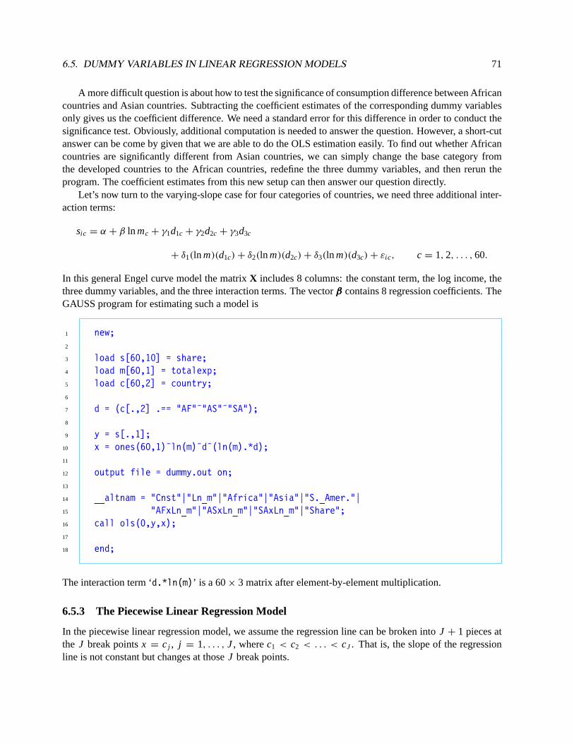
6.5. DUMMY VARIABLES IN LINEAR REGRESSION MODELS 71
A more difficult question is about how to test the significance of consumption difference between Africancountries and Asian countries. Subtracting the coefficient estimates of the corresponding dummy variablesonly gives us the coefficient difference. We need a standard error for this difference in order to conduct thesignificance test. Obviously, additional computation is needed to answer the question. However, a short-cutanswer can be come by given that we are able to do the OLS estimation easily. To find out whether Africancountries are significantly different from Asian countries, we can simply change the base category fromthe developed countries to the African countries, redefine the three dummy variables, and then rerun theprogram. The coefficient estimates from this new setup can then answer our question directly.
Let’s now turn to the varying-slope case for four categories of countries, we need three additional inter-action terms:
sic = α + β ln mc + γ1d1c + γ2d2c + γ3d3c
+ δ1(ln m)(d1c)+ δ2(ln m)(d2c)+ δ3(ln m)(d3c)+ εic, c = 1,2, . . . ,60.
In this general Engel curve model the matrixX includes 8 columns: the constant term, the log income, thethree dummy variables, and the three interaction terms. The vectorβββ contains 8 regression coefficients. TheGAUSS program for estimating such a model is
1 new;2
3 load s[60,10] = share;4 load m[60,1] = totalexp;5 load c[60,2] = country;6
7 d = (c[.,2] .== "AF"˜"AS"˜"SA");8
9 y = s[.,1];10 x = ones(60,1)˜ln(m)˜d˜(ln(m).*d);11
12 output file = dummy.out on;13
14 __altnam = "Cnst"|"Ln_m"|"Africa"|"Asia"|"S._Amer."|15 "AFxLn_m"|"ASxLn_m"|"SAxLn_m"|"Share";16 call ols(0,y,x);17
18 end;
The interaction term ‘d.*ln(m)’ is a 60× 3 matrix after element-by-element multiplication.
6.5.3 The Piecewise Linear Regression Model
In the piecewise linear regression model, we assume the regression line can be broken intoJ + 1 pieces atthe J break pointsx = c j , j = 1, . . . , J, wherec1 < c2 < . . . < cJ . That is, the slope of the regressionline is not constant but changes at thoseJ break points.

72 CHAPTER 6. RELATIONAL OPERATORS AND LOGIC OPERATORS
To construct a piecewise linear regression model, we need to defineJ dummy variables as follows:
d j i =
{1, for j ≤ k,
0, for j > k,if ck < xi ≤ ck+1, for k = 0, . . . , J,
wherec0 = −∞ andcJ+1 = ∞.Given a column vector of data ‘x0’ on the single explanatory variablexi and a column vector ‘c’ of J
break points, then × J matrix containing allJ dummy variablesd1i , d2i , . . ., dJ i can be created quite easilyin GAUSS as follows:
1 dum = (x0 .>= c’);
Here, if thei -th element of the vector ‘x0’ is greater than thej -th element but not greater than thej + 1-thelement of the vector ‘c’ , then the firstj elements in thei -th row of the matrix ‘dum’ are all 1’s and the lastJ − j elements are all 0’s.
1. If we assume the piecewise regression line is continuous, then
yi = α + βxi +
J∑j =1
γ j (xi − c j )d j i + εi ,
=
α + βxi + εi , if xi ≤ c1,(α −
k∑j =1
γ j c j
)+
(β +
k∑j =1
γ j
)xi + εi , if ck < xi ≤ ck+1, for k = 1, . . . , J.
Given the matrix ‘dum’ containing theJ dummy variablesd1i , d2i , . . ., dJ i , the matrix ‘x’ of allexplanatory variables for the present case is defined to be:
1 x = ones(n,1)˜x0˜((x0 - c’).*dum);
which is ann × (J + 2) matrix.
2. If we allow the piecewise regression line to be disconnected at thoseJ break points, then
yi = α + βxi +
J∑j =1
γ j (xi − c j )d j i +
J∑j =1
δ j d j i + εi ,
=
α + βxi + εi , if xi ≤ c1,(α −
k∑j =1
γ j c j +
k∑j =1
δ j
)+
(β +
k∑j =1
γ j
)xi + εi , if ck < xi ≤ ck+1, for k = 1, . . . , J,
where the parameterδ j indicates the distance between the adjacent two pieces at the break pointx = c j . Given the matrix ‘dum’, the matrix ‘x’ of all explanatory variables for the present case is

6.5. DUMMY VARIABLES IN LINEAR REGRESSION MODELS 73
1 x = ones(n,1)˜x0˜((x0 - c’).*dum)˜dum;
which is ann × (2J + 2) matrix.

74 CHAPTER 6. RELATIONAL OPERATORS AND LOGIC OPERATORS

Chapter 7Iteration with Do-Loops
When we implement econometric methods in GAUSS programming, a very common situation is that weneed to repeat similar computation with almost identical sets of GAUSS commands. The process of iteratingthe same set of commands can be done by a mechanism called do-loop in GAUSS. We will explain theconcept of a do-loop through a simple example.
7.1 Do-loops
Consider the product of two column-vectors, says, ‘a’ and ‘b’, both with 5 elements. It is defined to bethe sum of the five products of the corresponding elements in ‘a’ and ‘b’. Suppose we want to use thisdefinitional formula to compute the product ‘c’ of two vectors, then the most straightforward way to do it is
1 c = a[1]*b[1] + a[2]*b[2] + a[3]*b[3] + a[4]*b[4] + a[5]*b[5];
This computation involves adding terms repeatedly with a sequential indices running from 1 to 5. This kindof arithmetic can always be written in arecursivefashion as follows:
1 c = 0;2 c = c + a[1]*b[1];3 c = c + a[2]*b[2];4 c = c + a[3]*b[3];5 c = c + a[4]*b[4];6 c = c + a[5]*b[5];
We note that the last five expressions are identical except the indices running from 1 to 5. In GAUSS anygroup of recursive expressions can be replaced by a do-loop.
A do-loop starts with the command ‘do until’, followed by a condition (the so-calleddo-loop con-dition), then a set of commands to be repeated, and then ends with the ‘endo’ command. The GAUSSstatements between the ‘do until’ command and the ‘endo’ command will be executed repeatedly. Aftereach iteration the do-loop condition will be checked to decide whether to continue another round of iterationor to stop. Iteration will be continued as long as the do-loop conditionis not satisfied. For the previousexample, we can use the following do-loop representation:
1 c = 0;2 i = 1;3 do until i > 5;4 c = c + a[i]*b[i];
75

76 CHAPTER 7. ITERATION WITH DO-LOOPS
5 i = i + 1;6 endo;
There is another kind of do-loops that start with the command ‘do while’. Though the basic structureis the same as that of the ‘do until’ command, the GAUSS statements between the ‘do while’ commandand the ‘endo’ command will be executed repeatedly as long as the do-loop conditionis still satisfied. Withthis command, the previous example can be written as
1 c = 0;2 i = 1;3 do while i <= 5;4 c = c + a[i]*b[i];5 i = i + 1;6 endo;
Generally speaking, there are two kinds of do-loop conditions: one involves an index, such as ‘i’ inthe previous examples, whose value has to be initiated before the do-loop and will change sequentiallyinside the do-loop. Iteration will stop when the index attains a prescribed value. The second type of do-loopconditions involve the computation result directly from each iteration, in which case iteration will stop whenthe computation result satisfies a prescribed criterion. For example, the iteration terminates when a resultinside the do-loop becomes smaller than 0.00001.
Do-loops can be nested; i.e., a do-loop can be placed inside another do-loop. Let’s consider the exampleof multiplying a matrix with a vector:Ab = c, whereA is ann × m matrix,b anm × 1 column vector, andthe resultc is ann × 1 column vector. If we want to conduct this computation with do-loops, then nesteddo-loops are needed. Other than computing the sum ofm products for each row ofA which requires onedo-loop (the inner do-loop), we need another layer of do-loop (the outer do-loop) for then rows ofA. Giventhe matrix ‘a’ and the vector ‘b’, we compute the vector ‘c’ as follows:
1 c = zeros(n,1);2 i = 1;3 do until i > n;4 j = 1;5 do until j > m;6 c[i] = c[i] + a[i,j]*b[j];7 j = j + 1;8 endo;9 i = i + 1;
10 endo;
It is important to note that in the very first statement we define the dimension of the ‘c’ vector to “reserve”the space for the iteration results. Such a technique is needed whenever we need to retain results from eachiteration. An alternative way of retaining results from each iteration, without the knowledge of how muchspace to be reserved, is as follows:

7.1. DO-LOOPS 77
1 c = 0;2 i = 1;3 do until i > n;4 j = 1;5 temp = 0;6 do until j > m;7 temp = temp + a[i,j]*b[j];8 j = j + 1;9 endo;
10 c = c|temp;11 i = i + 1;12 endo;13 c = c[2:rows(c)];
Here, a scalar ‘c’ is initiated with the value 0 right before the do-loop. We use this ‘c’ as a base and we willattach the result form each iteration to it. Each time the inner do-loop for computing the sum ofm productsis completed, the result is attached to ‘c’. After all n computations are finished, we have a(n + 1) × 1column vector ‘c’ whose first element needs to be deleted as is done in the statement right after the ‘endo’command. Note that if the result from each iteration is a vector (instead of a scalar as in the above example),then a vector has to be initiated before the do-loop so that the resulting vector from each iteration can beproperly attached to this initial vector.
A General Principle in Using Do-loop Do-loop is a useful tool in many situations. As a matter of fact, allthe matrix operations, such as matrix multiplication in the previous examples, can be replaced by do-loops.However, in most matrix operations we should use the matrix operators instead of do-loops. This is becausematrix operators are easier to use and are executed with much more efficiency. A general principle forGAUSS programming is thatthe use of do-loops should be avoided unless there is absolutely no alternative.Replacing do-loops with ingenious matrix operations, if possible, always save us tremendous amount ofcomputing time.
An Example Our previous program for the demand estimation can deal with one commodity only. Weneed to rerun that program ten times for the ten commodities of the International Consumption Data. Here,by using do-loops we can easily conduct the estimations for all ten commodities in one program. In such aprogram it is then straightforward to collect all the regression coefficient estimates and perform additionalcomputations with them. In particular, we can compute income elasticities for all ten commodities and forall 60 countries in one stroke. We can also check whether the sum of the ten intercept estimates is equal toone and whether the sums of the ten sets of all other coefficient estimates are equal to zero.
1 new;2
3 load q[60,10] = volume;4 load s[60,10] = share;5 load m[60,1] = totalexp;

78 CHAPTER 7. ITERATION WITH DO-LOOPS
6
7 p = (s.*m)./q;8 x = ln(m)˜ln(p);9
10 output file = all.out reset;11
12 __altnam = "Cnst"|"Ln_m"|"Food"|"Bev_tob"|"Clothing"|"Rent"|"HouseFur"|13 "Medicare"|"Transpt"|"Recreatn"|"Educatn"|"Other"|"Food_S";14
15 bout = zeros(1,12); /* Initializing a row vector to which all the16 regression coefficient estimates from the17 do-loop can attach. */18
19 eout = zeros(60,1); /* Initializing a column vector to which all20 the elasticities estimates from the do-loop21 can attach. */22
23 i = 1; /* Initializing an index for counting. */24 do until i > 10; /* Do-loop will run ten times. */25
26 y = s[.,i]; /* The index i picks one commodity in turn. */27 {vnam,mmt,b,stb,vb,seb,s2,cor,r2,e,d} = ols(0,y,x);28 eta = 1 + b[2]./s[.,i]; /* The computation of the elasticities. */29 bout = bout|b’; /* Collecting the regression estimates row by row. */30 eout = eout˜eta; /* Collecting the elasticity estimates column by31 column. */32 i = i + 1;33 endo;34 bout = bout[2:rows(bout),.]; /* Deleting unwanted first row. */35 eout = eout[.,2:cols(eout)]; /* Deleting unwanted first column. */36
37 eout = seqa(1,1,60)˜eout; /* Attaching a column of counters. */38
39 " The income elasticities for the ten commodities and 60 countries:";?;40 call printfm(eout,ones(1,11),"*.*lf"˜4˜0|(ones(10,1).*("*.*lf"˜6˜3));?;?;41
42 " The sum of ten sets of regression coefficient estimates:";?;43 format /rd 15,8; sumc(bout);44
45 end;
Note that after the ‘eout’ matrix is generated toward the end of the program, a column of 60 consecutivenumbers 1,2,. . .,60, which serve as counters are generated and attached to the ‘eout’ matrix to facilitate itsreading. We then print these counters in the first column of ‘eout’ as integers while the rest 60× 10 matrixof elasticity estimates as real numbers. Because different columns of ‘eout’ are to be printed differently, we

7.1. DO-LOOPS 79
must use a ‘printfm’ command, in which the second argument, a row of 11 ones, indicates all 11 columnsof ‘eout’ are numbers (instead of characters). The third argument of the ‘printfm’ command is a 11× 3formatting matrix. The first row of the formatting matrix, ‘*.*lf˜4˜0’, is associated with the first column of‘eout’, which contains the counters, and the other 10 rows are all identically equal to ‘(*.*lf ˜6˜3)’ sincethe last ten columns of ‘eout’ are to be printed in the same format. Note that the way we construct the lastten rows of the formatting matrix is based on an element-by-element trick for duplication. This trick can bequite useful in many occasions.
Breaking Away from Do-loop Sometimes we need to break away from the do-loop before the do-loopcondition is satisfied by using a supplementary GAUSS statement ‘break’. For a trivial example, if we onlywant to add the first three product terms from the original 5-iteration do-loop condition, then we put an ‘if’statement inside the loop as follows:
1 c = 0;2 i = 1;3 do until i > 5;4 if i > 3;5 break;6 endif;7 c = c + a[i]*b[i];8 i = i + 1;9 endo;
When the ‘if’ condition is satisfied (i.e., after three iterations are completed and the index ‘i’ becomes 4),then the ‘break’ statement is executed and the program will jump out of the loop and go to the statementimmediately after the ‘endo’ statement.
There is another supplementary GAUSS statement – the ‘continue’ statement – that help bypass someof the statements inside the do-loop but still continue the do-loop iteration as illustrated by the followingexample in which the third product term is to be skipped from the summation:
1 c = 0;2 i = 1;3 do until i > 5;4 if i == 3;5 continue;6 endif;7 c = c + a[i]*b[i];8 i = i + 1;9 endo;
When the ‘if’ condition is satisfied (i.e., after two iterations are completed and the index ‘i’ becomes 3) sothat the ‘continue’ statement is executed, the program will skip the rest of the statements inside the loopand jump to the top of the loop to evaluate the do-loop condition to decide whether to continue the iteration.The above program is equivalent to

80 CHAPTER 7. ITERATION WITH DO-LOOPS
1 c = a[1]*b[1] + a[2]*b[2] + a[4]*b[4] + a[5]*b[5];
where the third product is omitted.
7.2 Some Statistics Related to the OLS Estimation
In this section we briefly introduce a few estimators and test statistics that are used to deal with some com-mon problems with the OLS Estimation when data cannot really satisfy the standard assumptions requiredby the linear regression model. We then present GAUSS programs for those estimators and test statistics. Inparticular, we demonstrate how do-loops are necessary in many of these programs.
7.2.1 The Heteroscedasticity Problem
Heteroscedasticity is a problem with a linear regression modely = Xβββ + εεε in that Var(yi ) = Var(εi ) = σ 2i
are not constant acrossi so that
Var(εεε) =
σ 21 0 · · · 0
0 σ 22 · · · 0
......
. . ....
0 0 · · · σ 2n
≡ 666.
Heteroscedasticity usually occurs to the cross-section data.
White’s Estimator: The main problem with the OLS estimatorb under heteroscedasticity is that itsvariance-covariance matrix becomes more complicated:
Var(b) = (X′X)−1X′666X(X′X)−1= (X′X)−1
(n∑
i =1
σ 2i xi x′
i
)(X′X)−1,
wherex′
i is thei th row of then × k matrix X. However, the above expression can be consistently estimatedby the so-called White’s heteroscedasticity-consistent estimator:
Var(b) = (X′X)−1
(n∑
i =1
e2i xi x′
i
)(X′X)−1,
whereei are the OLS residuals.Given then × k data matrix ‘x’ of the explanatory variables and then-vector of OLS residuals ‘e’,
White’s heteroscedasticity-consistent estimator can be calculated by the GAUSS statement:
1 w_vb = invpd(x’x)*x’diagrv(eye(n),e)*x*invpd(x’x);

7.2. SOME STATISTICS RELATED TO THE OLS ESTIMATION 81
where the GAUSS command ‘diagrv’ takes two inputs – the first input is a square matrix and the secondone is a column vector – and produces a square matrix that is the same as the first input except the diagonalelements are those of the second input. Recall that the GAUSS command ‘eye(n)’ gives ann × n identitymatrix.
It is easy to verify that, given anyn × 1 column vector ‘a’ and n × n matrix ‘b’, the expression‘a.*b’ yields the same result as that of ‘diagrv(eye(n),a)*b’. Consequently, White’s heteroscedasticity-consistent estimator can be calculated by the following alternative GAUSS program:
1 w_vb = invpd(x’x)*x’(e.*x)*invpd(x’x);
White’s Test for Heteroscedasticity Given R2 of the special regression of the squared OLS residualse2i
on all the explanatory variables and their squared and cross product terms, White’s Test is based on thestatistic
Sw = n·R2,
wheren is the sample size. Suppose the number of the explanatory variables in such a regression isk◦, thenthe test statistic Sw has aχ2(k◦ − 2) distribution under the null hypothesis ofno heteroscedasticity.
The GAUSS program for calculating White’s test statistic is somewhat complicated. Given the samplesize ‘n’, the n × k data matrix ‘x’ of the explanatory variables including the constant term, and then-vectorof OLS residuals ‘e’, we use
1 j = 1;2 do until j > k;3 x0 = x0˜(x[.,j].*x[.,j:k]);4 j = j + 1;5 endo;6
7 y0 = eˆ2;8 e0 = y0 - x0*invpd(x0’x0)*x0’y0;9 tss0 = (y0 - meanc(y0))’(y0 - meanc(y0));
10 rss0 = e0’e0;11 r2 = (tss0 - rss0)/tss0;12
13 s_w = n*r2;
Here, a do-loop is necessary in the construction of the ‘x0’ matrix which contains the data on all the ex-planatory variables in ‘x’ and their squared and cross product terms. The five statements after the do-looprepresent the standard procedure to compute R2 where the particular dependent variable ‘y0’ in this compu-tation is the squared OLS residuale2
i . White’s test statistic is in ‘s_w’. If the computed value of White’s teststatistic is greater than the(1 − α)% critical point from theχ2(k◦ − 2) distribution, wherek◦ is the columnnumber of ‘x0’, then the null hypothesis ofno heteroscedasticity will be rejected.

82 CHAPTER 7. ITERATION WITH DO-LOOPS
Breusch-Pagan’s Test for Heteroscedasticity If heteroscedasticity follows the form
σ 2i = σ 2
·h(z′
i γγγ ),
for some known functionh of some vectorzi of p observable variables which includes the constant termand can overlap withxi , then Breusch-Pagan’s test statistic is
SBP =(w − 1n)
′Z(Z′Z)−1Z′(w − 1n)
(w − 1n)′(w − 1n)/n.
where1n is n dimensional vector of ones,w andZ are then × 1 vector and then × p matrix containing allthe observations ofwi andzi , respectively. Here,wi are normalized squared residuals
wi =e2
i1n
∑nj =1 e2
j
.
SBP has theχ2(p − 1) distribution under the null hypothesis and the normality assumption.Given then × k data matrix ‘x’ of the explanatory variables, then × p data matrix ‘z’ of the variables
zi , and then-vector of OLS residuals ‘e’, the GAUSS program for calculating Breusch-Pagan’s test statisticis
1 w = eˆ2./meanc(eˆ2);2 s_bp = (w - 1)’z*invpd(z’z)*z’(w - 1)/((w - 1)’(w - 1)/n);
We note that although ‘w’ is an n-dimensional vector, we can still subtract a scalar 1 from it since GAUSSwill automatically expand 1 to ann-vector of ones which becomes conformable to ‘w’.
7.2.2 The Autocorrelation Problem
In a linear regression model for time-series data (here, we change the subscript fromi to t to emphasize thenature of data is time series):
yt = x′
tβββ + εt , t = 1, . . . ,n,
we usually expect nonzero covariances of the disturbances across time
Cov(ys, yt) = Cov(εs, εt) ≡ cst 6= 0, for some s, t = 1,2, . . . ,n.
Because of these nonzero covariances the OLS estimation has the problem that the variance of the OLSestimatorb changes from the formulaσ 2(X′X)−1 to
Var(b) = (X′X)−1
(n∑
s=1
n∑t=1
cstxsx′
t
)(X′X)−1,
wherex′
t is thet th row of then × k matrixX.
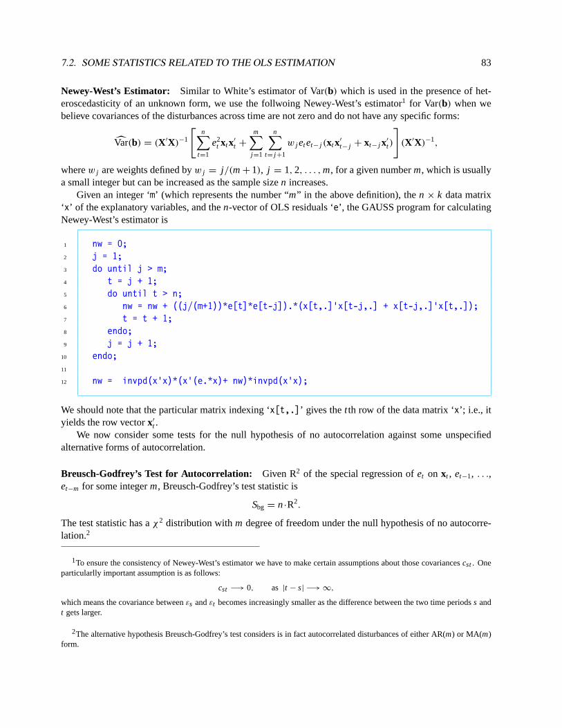
7.2. SOME STATISTICS RELATED TO THE OLS ESTIMATION 83
Newey-West’s Estimator: Similar to White’s estimator of Var(b) which is used in the presence of het-eroscedasticity of an unknown form, we use the follwoing Newey-West’s estimator1 for Var(b) when webelieve covariances of the disturbances across time are not zero and do not have any specific forms:
Var(b) = (X′X)−1
[n∑
t=1
e2t xtx′
t +
m∑j =1
n∑t= j +1
w j etet− j (xtx′
t− j + xt− j x′
t)
](X′X)−1,
wherew j are weights defined byw j = j/(m+ 1), j = 1,2, . . . ,m, for a given numberm, which is usuallya small integer but can be increased as the sample sizen increases.
Given an integer ‘m’ (which represents the number “m” in the above definition), then × k data matrix‘x’ of the explanatory variables, and then-vector of OLS residuals ‘e’, the GAUSS program for calculatingNewey-West’s estimator is
1 nw = 0;2 j = 1;3 do until j > m;4 t = j + 1;5 do until t > n;6 nw = nw + ((j/(m+1))*e[t]*e[t-j]).*(x[t,.]’x[t-j,.] + x[t-j,.]’x[t,.]);7 t = t + 1;8 endo;9 j = j + 1;
10 endo;11
12 nw = invpd(x’x)*(x’(e.*x)+ nw)*invpd(x’x);
We should note that the particular matrix indexing ‘x[t,.]’ gives thet th row of the data matrix ‘x’; i.e., ityields the row vectorx′
t .We now consider some tests for the null hypothesis of no autocorrelation against some unspecified
alternative forms of autocorrelation.
Breusch-Godfrey’s Test for Autocorrelation: Given R2 of the special regression ofet on xt , et−1, . . .,et−m for some integerm, Breusch-Godfrey’s test statistic is
Sbg = n·R2.
The test statistic has aχ2 distribution withm degree of freedom under the null hypothesis of no autocorre-lation.2
1To ensure the consistency of Newey-West’s estimator we have to make certain assumptions about those covariancescst. Oneparticularlly important assumption is as follows:
cst −→ 0, as |t − s| −→ ∞,
which means the covariance betweenεs andεt becomes increasingly smaller as the difference between the two time periodss andt gets larger.
2The alternative hypothesis Breusch-Godfrey’s test considers is in fact autocorrelated disturbances of either AR(m) or MA(m)form.

84 CHAPTER 7. ITERATION WITH DO-LOOPS
Given the sample size ‘n’, the n × k data matrix ‘x’ of the explanatory variables, and then-vector ofOLS residuals ‘e’, the GAUSS program for calculating Breusch-Godfrey’s test statistic is
1 x0 = x˜shiftr(ones(m,1)*e’,seqa(1,m),0)’;2 y0 = e;3
4 e0 = y0 - x0*invpd(x0’x0)*x0’y0;5 tss0 = (y0 - meanc(y0))’(y0 - meanc(y0));6 rss0 = e0’e0;7 r2 = (tss0 - rss0)/tss0;8
9 s_w = n*r2;
The most interesting part of the program is in the first line where then × (k + m) matrix of explanatoryvariables is constructed. There we use a new GAUSS command ‘shiftr’ which takes three inputs: the firstinput is anm × n matrix, say, ‘a’, the second input is anm × 1 column vector, say, ‘b’, and the third inputis either anm × 1 column vector or a scalar, say, ‘c’. What the command ‘shiftr’ does is to shift the rowsof the matrix ‘a’ horizontally. The number of steps shifted in each row is determined by the value in thecorresponding element in the vector ‘b’. If the number is positive, then the shift is to the right. Otherwise,the shift is to the left. For example, if the third element in ‘b’ is 5, then the third row of ‘a’ is shifted fivesteps to the right so that the last five numbers in that row will be lost while the first five numbers are all thenumber in the third element of the third input vector ‘c’. Going back to the above program, we see that thefirst input for the command ‘shiftr’ is an m × n matrix with the identical row ‘e’ and the second inputis a column vector of sequential integers from 1 tom. The output of that command is anm × n matrix asfollows:
0 e1 e2 e2 · · · em em+1 em+2 · · · en−1
0 0 e1 e2 · · · em−1 em em+1 · · · en−2
0 0 0 e1 · · · em−2 em−1 em · · · en−3
......
......
. . ....
......
...
0 0 0 0 · · · e1 e2 e2 · · · en−m
.
The first row is shifted to the right by one step (so that the last elementen is pushed off) while themth rowis shifted to the right bym steps. All the spaces left are filled with zero (which is specfied in the third inputof the ‘shiftr’ command.
Finally, we note that the output of the command ‘shiftr’ is transposed to ann × m matrix beforeconcatenated horizontally to then × k matrix ‘x’. It should be emphasized that the operation of transposehas higher priority than the operation of concatenation so that it is not necessary to add parentheses around‘shiftr(ones(m,1)*e’,seqa(1,m),0)’’.

7.2. SOME STATISTICS RELATED TO THE OLS ESTIMATION 85
Q Tests for Autocorrelation: Given the j th order sample autocorrelations from the OLS residuals:
ρ j =
n∑t= j +1
etet− j
n∑t=1
e2t
,
we have the following two test statistics for a given integerm:
1. Box-Pierce Q Statistic:
Q1 = nm∑
j =1
ρ 2j .
2. Ljung-Box Q Statistic:
Q2 = n(n + 2)m∑
j =1
ρ 2j
n − j.
Both statistics have aχ2 distribution withm degree of freedom under the null hypothesis of no autocorrela-tion.
Given the sample size ‘n’, an integer ‘m’, and then-vector of OLS residuals ‘e’, the GAUSS programfor calculating Q test statistics is
1 rho = (shiftr(ones(m,1)*e’,seqa(1,m),0)*e)./(e’e);2 q1 = n*(rho’rho);3 q2 = n*(n + 2)*(rho’(rho./(n - seqa(1,m))));
7.2.3 Structural Stability
When we use Chow tests for structural changes, one basic assumption is that we know exactly when thestructural changes occur so that we can divide the sample accordingly. But in many applications usingtime-series datawe may not know whether there are structural changes and, if there are, when they occur. Inother words we are not certain about the structural stability, or the constancy of the regression coefficientsβββ, over time. To test structural stability of a linear regression modely = Xβββ + εεε, we use the CUSUM testwhich is based on theone-step ahead prediction errors:
e◦
t ≡ yt − x′
tbt−1, t = k + 1, k + 2, . . . ,n,
whereyt andxt are thet-th observation on the dependent variable and thek regressors, respectively. Herex′
tbt−1 can be considered as apredictorof yt based on the previoust−1 observations withbt−1 being definedby
bt−1 = (X′
t−1Xt−1)−1X′
t−1yt−1,
whereyt−1 is a (t − 1) × 1 vector containing the firstt − 1 observations on the dependent variable whileXt−1 is a(t − 1)× k matrix containing the firstt − 1 observations on the explanatory variables: Obviously,bt−1 is feasible only when the rank ofXt−1 is equal to the number of explanatory variablesk, i.e., when its

86 CHAPTER 7. ITERATION WITH DO-LOOPS
row number is no less thank. So we can computebt−1, and therefore the recursive residualse◦
t , only fort = k + 1, k + 2, . . . ,n.
Let’s also define therescaled one-step ahead prediction errors:
wt ≡e◦
t√1 + x′
t(X′
t−1Xt−1)−1xt
, t = k + 1, k + 2, . . . ,n,
and their sample variance:
s2w ≡
1
n − k − 1
n∑t=k+1
(wt − w)2,
wherew ≡ (n − k)−1∑nt=k+1wt . The CUSUM test is based on the fact that, under the null hypothesis that
the regression coefficientsβββ are stable, the distribution of then − k statistics
C j ≡
j∑t=k+1
wt
sw, j = k + 1, k + 2, . . . ,n,
can be derived. In particular, we know the 90 %, 95 %, and 99 % critical values (denoted asψ0.05,ψ0.025, andψ0.005, respectively) of this distribution are 0.850, 0.948, and 1.143, respectively. To conduct the CUSUMtest at the(1 − α)% significance level, we check whether each point( j, C j ) lies inside the correspondingconfidence bound which is delimited by two straight lines that are symmetrical with respect to the horizontalaxis: one is the line connecting the two points:
(k, ψα/2
√n − k
)and
(n, 3ψα/2
√n − k
). The other is the
line connecting the two points:(k, −ψα/2
√n − k
)and
(n, −3ψα/2
√n − k
). The null hypothesis is rejected
if any of C j lies outside the corresponding confidence interval.Before writing a GAUSS program for calculating the CUSUM test statistics, we note that the computa-
tion repeatedly involves increasing matricesyt−1 andXt−1 and is hard to do in one stroke based on matrixalgebra technique only. So using do-loops appears the only way for the task. Now, given that then observa-tions on the dependent variable and thek regressors have been loaded into ‘y’ and ‘x’, respectively, then then − k CUSUM test statisticsC j can be computed by the following simple GAUSS program:
1 w = zeros(n-k,1);2 t = k+1;3 do until t > n;4 e = y[t] - x[t,.]*invpd(x[1:t-1,.]’x[1:t-1,.])*x[1:t-1,.]’y[1:t-1];5 w[t-k] = e/sqrt(1 + x[t,.]*invpd(x[1:t-1,.]’x[1:t-1,.])*x[t,.]’);6 t = t + 1;7 endo;8 s2 = (w - meanc(w))’(w - meanc(w))/(n-k-1);9 c = cumsumc(w./sqrt(s2));
‘c’ is an (n − k)× 1 vector containing the CUSUM test statisticsC j , for j = k + 1, k + 2, . . . ,n.In the above program we have used a new GAUSS command ‘cumsumc’. It takes one input which is
an(n − k) × 1 vector (of rescaled one-step ahead prediction errorswt ) and produced another vector of thesame size whose elements are the cumulative sums of the elements of the input vector. A similar GAUSScommand is ‘cumprodc’ which does cumulative products.
Finally, we note that to complete the testing procedure, we have to draw a graph for the confidencebound, which we will not do here.

Chapter 8GAUSS Procedures: Basics
Recall in section 5.5, the three parts of the GAUSS program for computing the three Chow test statisticsare almost identical. Each begins with the computation of two RSS (one for the restricted model and theother for the unrestricted model) and their respective degrees of freedom, then the test statistic and thecorresponding p-value. The only difference in these computations is the data that are used. We may wonderwhether there is a way in GAUSS to exploit the similarity in computations to save our programming chore.The answer is yes and the tool used for this purpose is called a procedure.
A procedure can be described in short as a group of GAUSS statements that is a self-contained unitresiding in the program that accepts inputs and produces outputs. Once a procedure is defined inside a pro-gram, it can be used or, in GAUSS terminology,calledrepeatedly with different inputs to produce differentoutputs. For example, the part of the program for each of the three Chow test statistics can be made as aprocedure. The inputs of such a procedure are three matrices: the vector of dependent variable, denoted as‘y’, the matrix of explanatory variables from the restricted model, denoted as ‘xr’, and the one from theunrestricted model, denoted as ‘xu’. The output is the p-value of the Chow test statistic. The procedure canbe formally written as follows:
1 proc (1) = chow(y,xr,xu);2
3 local rss_r, rss_u, df_r, df_u, f, p_value;4
5 rss_r = y’y - y’xr*invpd(xr’xr)*xr’y;6 df_r = rows(xr) - cols(xr);7
8 rss_u = y’y - y’xu*invpd(xu’xu)*xu’y;9 df_u = rows(xu) - cols(xu);
10
11 f = ((rss_r - rss_u)/(df_r - df_u))/12 (rss_u/df_u);13
14 p_value = cdffc(f,df_r-df_u,df_u);15
16 retp(p_value);17 endp;
Let’s take a look at the structure of this procedure, which can be broken into five components:
1. The first component starts with the GAUSS command ‘proc’ which initiates the definition of a proce-dure. The number in the first pair of parentheses indicates how many output matrices will be producedby this procedure. In our example there is one output – the p-value which is a scalar. The letters after
87

88 CHAPTER 8. GAUSS PROCEDURES: BASICS
the equality sign, such as ‘chow’, give the name of the procedure which follows the same naming rulefor variables. Whenever the procedure is needed, it will be called by this name. The arguments insidethe second pair of parentheses are inputs. In our example, there are three inputs ‘y’, ‘ xr’ and ‘xu’.
2. The second component starts with the GAUSS command ‘local’ followed by a list of variable names.All the variables used inside the procedure, except those input variables specified in the ‘proc’ state-ment (e.g., the three matrices ‘y’, ‘ xr’, and ‘xu’ in our example), are referred to as local variablesand should be listed in this ‘local’ statement. In general,all the variables that appear on the left-hand side of the GAUSS statements inside a procedure are local variables. In our example, six localvariables have been defined. The local statement may be omitted if no local variables are needed.
In contrast to the local variables inside a procedure, all variables defined and used outside proceduresare said to be global. The conceptual difference between local variables and global variables is quiteimportant and it will be elaborated further in section 8.2.
3. The third component is the main body of the procedure, which may contain any number of GAUSSexpressions that define the procedure. There are six expressions in our example.
4. The fourth component of the procedure is the ‘retp’ command that “returns” the output variablescreated by the procedure. Multiple output variables are possible and require multiple arguments in theparentheses. If there is no output variable to be returned, the ‘retp’ command may be omitted.
5. The last component is simply the ‘endp’ command that formally ends the definition of the procedures.
To use, or to call, the above procedure, we type the following command in the main program:
1 pv = chow(y,x1,x2);
where ‘x1’ and ‘x2’ are the matrices of explanatory variables from the restricted model and the unrestrictedmodel, respectively. Both of them and the vector of dependent variable ‘y’ should have been defined earlierin the main program.
The output is stored in the new matrix (here, it is a scalar) ‘pv’, which is the p-value for the Chow teststatistic. Note that the names of the input and output variables here are different from those used inside theprocedure. As a matter of fact, all local variables used inside a procedure are completely independent ofthe global variables used outside the procedure. Furthermore, the local names used inside a procedure canbe the same as some global names outside the procedure. GAUSS will understand they represent differentvariables. Also, all the global variables defined in a GAUSS program will remain in the memoryeven afterthe execution of the program is finished. But the local variables used inside a procedure will be erased fromthe memoryas soon as the execution of this procedure is completed.
It is possible for a procedure to have no output variable at all. In such a case the number inside thefirst pair of parentheses in the ‘proc’ command is ‘0’ and there is no need for the parentheses in the ‘retp’command. What this kind of procedures usually do is to make some computation and/or to print somethingon the screen (or into an ASCII output file). For example, the goal of the previous procedure ‘chow’ is tocompute the p-value of the Chow test statistic. The reason for deriving such a p-value is to eventually print itso that we can judge whether it is smaller than the designated size of the test, say, 5%, in which case the null

89
hypothesis of no structural change will be rejected. But we note GAUSS can also make such a judgment.What we really want is actually not the p-value per se but a decision of whether to reject the null. So we canrewrite the procedure in a way that it does not produce any matrix output but prints the testing decision.
1 proc (0) = chow_a(y,xr,xu);2
3 local rss_r, rss_u, df_r, df_u, f, p_value;4
5 rss_r = y’y - y’xr*invpd(xr’xr)*xr’y;6 df_r = rows(xr) - cols(xr);7
8 rss_u = y’y - y’xu*invpd(xu’xu)*xu’y;9 df_u = rows(xu) - cols(xu);
10
11 f = ((rss_r - rss_u)/(df_r - df_u))/12 (rss_u/df_u);13
14 p_value = cdffc(f,df_r-df_u,df_u);15
16 if p_value < 0.05;17 "The Null Hypothesis of No Structural Change Is Rejected!";18 else;19 "The Null Hypothesis of No Structural Change cannot be Rejected!";20 endif;21
22 endp;
Here, an ‘if...else...endif’ command is used to determine which testing result to be printed. Sincethere is no output variables, the number of output specified in the ‘proc’ command is set at 0, while the‘retp’ command is omitted. When such a procedure is needed, it is called by
1 call chow_a(y,x1,x2);
Let’s consider the case where the number of output variables is more than one. In such a case the callingstatement is a little different. Suppose in the original ‘chow’ procedure, besides the p-value, we also wantto output the test statistic ‘f’ and the two corresponding degrees of freedom, then we need the followingversion of the procedure that has four output variables:
1 proc (4) = chow_b(y,xr,xu);2
3 local rss_r, rss_u, df_r, df_u, f, p_value;4
5 rss_r = y’y - y’xr*invpd(xr’xr)*xr’y;6 df_r = rows(xr) - cols(xr);

90 CHAPTER 8. GAUSS PROCEDURES: BASICS
7
8 rss_u = y’y - y’xu*invpd(xu’xu)*xu’y;9 df_u = rows(xu) - cols(xu);
10
11 f = ((rss_r - rss_u)/(df_r - df_u))/12 (rss_u/df_u);13 p_value = cdffc(f,df_r-df_u,df_u);14
15 retp(f,df_r-df_u,df_u,p_value);16 endp;
The number of output specified in the ‘proc’ command is 4 and, correspondingly, there are four argumentsin the ‘retp’ command, among which we note the second argument itself is an expression. That is, thearguments of the ‘retp’ command can take the form of algebraic expressions. This extra flexibility helpscut the number of local variables needed in the procedure. To call the above procedure, we type
1 {t,df1,df2,pv} = chow_b(y,x1,x2);
Note that the four output variables ‘t’, ‘ df1’, ‘ df2’, and ‘pv’ are enclosed by a pair of braces. The structureof this statement is quite unique in GAUSS. It has more than one variableon the left-hand sideof the equalitysign.
Let’s now present a full example. Suppose in the estimation of the Engel curve model we are interestedin the difference between the developed and the developing countries. Since the data are not grouped intodeveloped and developing countries as the framework of the Chow test requires, we must rearrange thedata first. The original data needed are in the three ASCII files: ‘share’, ‘ totalexp’, and ‘country’. Inparticular, in the file ‘country’ there are two columns of characters: the first column contains the countries’names and the second one the continent codes: ‘AF’ (for Africa), ‘ AS’ (for Asia), ‘NA’ (for North America),‘SA’ (for South America), and ‘EU’ (for Europe). The continent codes are used to separate the developedcountries from the developing ones.
1 new;2
3 load s[60,10] = share;4 load m[60,1] = totalexp;5 load c[60,2] = country;6
7 y = s[.,1];8 x = ones(60,1)˜ln(m);9
10 /* Constructing an indicator for the developed countries. */11 ind = (c[.,2] .== "NA" .or c[.,2] .== "EU");12
13 /* Reorganizing the data matrices ‘y’ and ‘x’ with the data for the14 developed countries first, followed by the data for the developing

91
15 countries. */16 y = selif(y,ind)|delif(y,ind);17 x = selif(x,ind)|delif(x,ind);18
19 /* The number of the developed countries (the number of 1’s in the20 indicator.) */21 n1 = sumc(ind);22
23 /* The expanded matrix of explanatory variables for the case 1 model. */24 x1 = (ones(n1,1)˜zeros(n1,1)˜x[1:n1,2])|25 (zeros(n-n1,1)˜ones(n-n1,1)˜x[(n1+1):n,2]);26 /* The expanded matrix of explanatory variables for the case 2 model. */27 x2 = (x[1:n1,.]˜zeros(n1,2))|(zeros(n-n1,2)˜x[(n1+1):n,.]);28
29 format /rd 6,3;30
31 {test,df1,df2,pv} = chow_b(y,x,x1);32 " The Chow test statistic for testing the null hypothesis of";33 " no structural change against the case 1 model is " test;34 " The degrees of freedom are " df1;; " and " df2;35 " The corresponding p-value is " pv;36
37 {test,df1,df2,pv} = chow_b(y,x,x2);38 " The Chow test statistic for testing the null hypothesis of";39 " no structural change against the case 2 model is " test;40 " The degrees of freedom are " df1;; " and " df2;41 " The corresponding p-value is " pv;42
43 {test,df1,df2,pv} = chow_b(y,x1,x2);44 " The Chow test statistic for testing the null hypothesis of";45 " the case 1 model against the case 2 model is " test;46 " The degrees of freedom are " df1;; " and " df2;47 " The corresponding p-value is " pv;48
49 /*************************************************************************50 * The Definition of the Procedure ‘chow_b’. *51 *************************************************************************/52 proc (4) = chow_b(y,xr,xu);53
54 local rss_r, rss_u, df_r, df_u, f, p_value;55
56 rss_r = y’y - y’xr*invpd(xr’xr)*xr’y;57 df_r = rows(xr) - cols(xr);58
59 rss_u = y’y - y’xu*invpd(xu’xu)*xu’y;
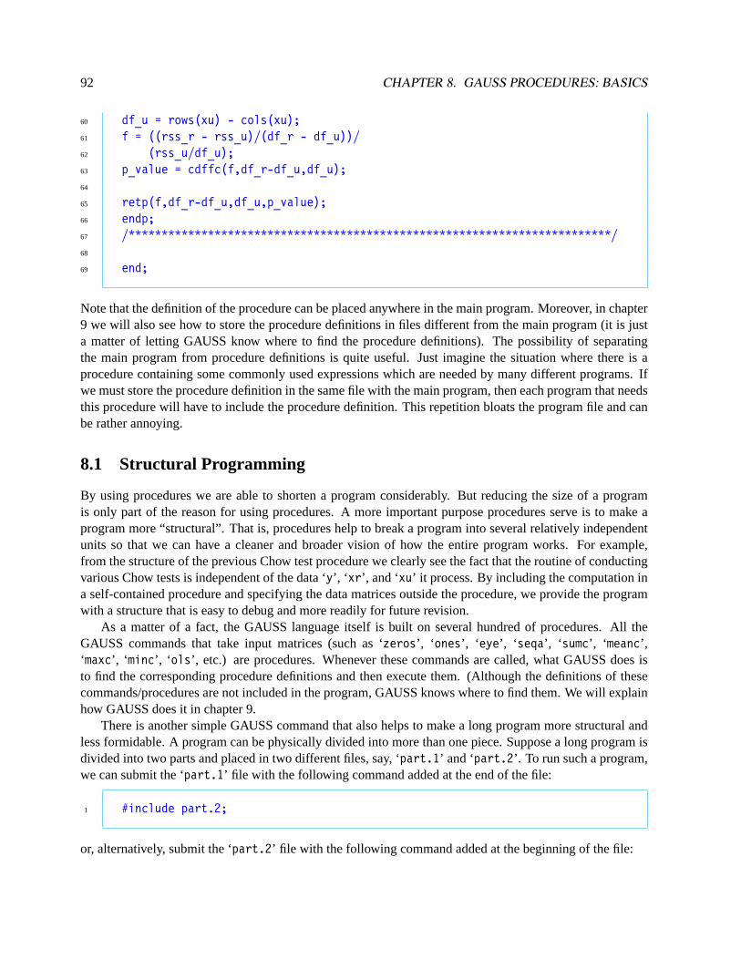
92 CHAPTER 8. GAUSS PROCEDURES: BASICS
60 df_u = rows(xu) - cols(xu);61 f = ((rss_r - rss_u)/(df_r - df_u))/62 (rss_u/df_u);63 p_value = cdffc(f,df_r-df_u,df_u);64
65 retp(f,df_r-df_u,df_u,p_value);66 endp;67 /*************************************************************************/68
69 end;
Note that the definition of the procedure can be placed anywhere in the main program. Moreover, in chapter9 we will also see how to store the procedure definitions in files different from the main program (it is justa matter of letting GAUSS know where to find the procedure definitions). The possibility of separatingthe main program from procedure definitions is quite useful. Just imagine the situation where there is aprocedure containing some commonly used expressions which are needed by many different programs. Ifwe must store the procedure definition in the same file with the main program, then each program that needsthis procedure will have to include the procedure definition. This repetition bloats the program file and canbe rather annoying.
8.1 Structural Programming
By using procedures we are able to shorten a program considerably. But reducing the size of a programis only part of the reason for using procedures. A more important purpose procedures serve is to make aprogram more “structural”. That is, procedures help to break a program into several relatively independentunits so that we can have a cleaner and broader vision of how the entire program works. For example,from the structure of the previous Chow test procedure we clearly see the fact that the routine of conductingvarious Chow tests is independent of the data ‘y’, ‘ xr’, and ‘xu’ it process. By including the computation ina self-contained procedure and specifying the data matrices outside the procedure, we provide the programwith a structure that is easy to debug and more readily for future revision.
As a matter of a fact, the GAUSS language itself is built on several hundred of procedures. All theGAUSS commands that take input matrices (such as ‘zeros’, ‘ ones’, ‘ eye’, ‘ seqa’, ‘ sumc’, ‘ meanc’,‘maxc’, ‘ minc’, ‘ ols’, etc.) are procedures. Whenever these commands are called, what GAUSS does isto find the corresponding procedure definitions and then execute them. (Although the definitions of thesecommands/procedures are not included in the program, GAUSS knows where to find them. We will explainhow GAUSS does it in chapter 9.
There is another simple GAUSS command that also helps to make a long program more structural andless formidable. A program can be physically divided into more than one piece. Suppose a long program isdivided into two parts and placed in two different files, say, ‘part.1’ and ‘part.2’. To run such a program,we can submit the ‘part.1’ file with the following command added at the end of the file:
1 #include part.2;
or, alternatively, submit the ‘part.2’ file with the following command added at the beginning of the file:

8.2. ACCESSING GLOBAL VARIABLES DIRECTLY 93
1 #include part.1;
When a file is ‘included’, it is literally plugged into the place where it is ‘included’. With this technique,it becomes possible to divide a long program into a few logically separable components and then ‘include’them back into one program.
8.2 Accessing Global Variables Directly
Earlier when we discussed the ‘local’ statement, we mentioned that variables used inside the proceduredefinition were either inputs specified in the ‘proc’ statement or local variables declared by the ‘local’statement. However, this statement is not exactly accurate. There is an important exception: all the globalvariables defined in the main program, but before the procedure is called, can be referred to and used insidethe procedure definitions, given that the names of global variables do not conflict with any of the localvariables.
For example, when we define ‘chow_b’ procedure, we do not really need to list the vector of dependentvariable ‘y’ in the ‘proc’ command. That is, the following expression in that example
1 proc (4) = chow_b(y,xr,xu);
can be simplified to
1 proc (4) = chow_b(xr,xu);
The program will still work as long as the global variable ‘y’ is properly defined before calling this newversion of the procedure. That is, the global variable ‘y’ can be referenced inside this new version of‘chow_b’ just like the input variables or local variables. However, it should be emphasized that if ‘y’ has notbeen suitably defined before the procedure is called, then an error message will ensue.
The possibility of accessing global variables directly from inside a procedure helps to reduce the numberof input variables necessarily specified in the ‘proc’ statement. But we should also note that such a practicemakes a procedure less self-contained and therefore causes potential problems. Unlike the inputs or the localvariables, which are explicitly specified in the ‘proc’ and the ‘local’ statements, the use of global variablesusually is not clearly indicated in the procedure definition. So it is very easy to forget defining those globalvariables properly before calling the procedure. It is not hard to imagine how much trouble may happen toa long program containing hundreds of global variables and dozens of procedures trying to access variousglobal variables. Nevertheless, in section 9.7 we will see there are some advanced commands in GAUSS(the ‘external’ and ‘declare’ commands) that help alleviate this difficulty.
Earlier when we discussed the ‘ols’ command in section 5.3, we mentioned the concept of “switches”and presented three of them: ‘__con’, ‘ __altnam’, and ‘_olsres’. We also indicated that the ‘ols’ com-mand, like many other GAUSS commands, was in fact a procedure. What we have been saying in thissection is that all the procedures, certainly including the ‘ols’ command, can access global variables. Whatwe called “switches” earlier are nothing but global variables which are accessed from inside the definition

94 CHAPTER 8. GAUSS PROCEDURES: BASICS
of the ‘ols’ procedure. The function of these global variables is, as mentioned before, to control someaspect of the OLS computation. These global variables have their default values, but can be redefined beforecalling the ‘ols’ procedure.
Here a technical question arises: as we indicated before, the global variables must be prepared properlyand explicitly before calling the procedure which accesses those global variables. But we also said that wedo not really need to include the explicit definitions of the global variables, such as ‘__con’, ‘ __altnam’,and ‘_olsres’, before we call the ‘ols’ procedure. How can this omission be allowed? Moreover, how arethe default values of those global variables are defined? These questions will be answered in section 9.7 .
The above analysis of the global variables for the ‘ols’ command should also demonstrate why theability of procedures to access the global variables is useful. If all those global variables, which allow usto conveniently control the execution of the ‘ols’ procedure, need to be defined as the input variables andlisted in the ‘proc’ statement, then every time we call the ‘ols’ command, we have to specify all of themexplicitly even though most of the time their values do not need to be changed. Repeatedly doing so can bequite annoying and prone to mistakes.
8.3 Calling Other Procedures in a Procedure
It is quite conceivable that the definition of a procedure may get too long to be comprehensible. So theremay be a need to make part of a long procedure another self-contained procedure. Dealing with this kindof multi-level procedures actually is quite easy in GAUSS. All we have to do is in the first procedure to (1)include the name of the second procedure in the ‘proc’ statement; and (2) declare this name as a procedurein the ‘local’ statement. With these minor modification in the first procedure and no special treatment atall in the second procedure, we can call the second procedure from inside the first procedure just like callingthe first procedure from the main program.
Let’s go back to the program of the three Chow tests. We will try to rewrite that program to demonstratehow the multi-level procedures can be used (although this change does not help simplify the program andappears unnecessary). Specifically, we will make the second part of that program a self-contained procedure,with the name ‘testing’, which calls the original procedure ‘chow_b’. That is, the main program, whichbecomes quite short, will call the procedure ‘testing’, while the procedure ‘testing’ will call the secondprocedure ‘chow_b’.
1 new;2
3 load s[60,10] = share;4 load m[60,1] = totalexp;5 load c[60,2] = country;6
7 y = s[.,1];8 x = ones(60,1)˜ln(m);9
10 ind = (c[.,2] .== "NA" .or c[.,2] .== "EU");11 n1 = sumc(ind);12
13 y = selif(y,ind)|delif(y,ind);
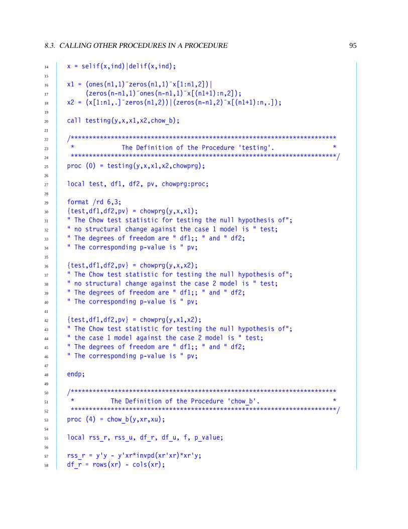
8.3. CALLING OTHER PROCEDURES IN A PROCEDURE 95
14 x = selif(x,ind)|delif(x,ind);15
16 x1 = (ones(n1,1)˜zeros(n1,1)˜x[1:n1,2])|17 (zeros(n-n1,1)˜ones(n-n1,1)˜x[(n1+1):n,2]);18 x2 = (x[1:n1,.]˜zeros(n1,2))|(zeros(n-n1,2)˜x[(n1+1):n,.]);19
20 call testing(y,x,x1,x2,chow_b);21
22 /*************************************************************************23 * The Definition of the Procedure ‘testing’. *24 *************************************************************************/25 proc (0) = testing(y,x,x1,x2,chowprg);26
27 local test, df1, df2, pv, chowprg:proc;28
29 format /rd 6,3;30 {test,df1,df2,pv} = chowprg(y,x,x1);31 " The Chow test statistic for testing the null hypothesis of";32 " no structural change against the case 1 model is " test;33 " The degrees of freedom are " df1;; " and " df2;34 " The corresponding p-value is " pv;35
36 {test,df1,df2,pv} = chowprg(y,x,x2);37 " The Chow test statistic for testing the null hypothesis of";38 " no structural change against the case 2 model is " test;39 " The degrees of freedom are " df1;; " and " df2;40 " The corresponding p-value is " pv;41
42 {test,df1,df2,pv} = chowprg(y,x1,x2);43 " The Chow test statistic for testing the null hypothesis of";44 " the case 1 model against the case 2 model is " test;45 " The degrees of freedom are " df1;; " and " df2;46 " The corresponding p-value is " pv;47
48 endp;49
50 /*************************************************************************51 * The Definition of the Procedure ‘chow_b’. *52 *************************************************************************/53 proc (4) = chow_b(y,xr,xu);54
55 local rss_r, rss_u, df_r, df_u, f, p_value;56
57 rss_r = y’y - y’xr*invpd(xr’xr)*xr’y;58 df_r = rows(xr) - cols(xr);

96 CHAPTER 8. GAUSS PROCEDURES: BASICS
59
60 rss_u = y’y - y’xu*invpd(xu’xu)*xu’y;61 df_u = rows(xu) - cols(xu);62 f = ((rss_r - rss_u)/(df_r - df_u))/63 (rss_u/df_u);64 p_value = cdffc(f,df_r-df_u,df_u);65
66 retp(f,df_r-df_u,df_u,p_value);67 endp;68
69 end;
Obviously, what the procedure ‘testing’ does is simply calling the second procedure ‘chow_b’ (using thelocal name ‘chowprg’) three times and printing the testing results. What the main program does is to preparethe four data matrices ‘y’, ‘ x’, ‘ x1’, and ‘x2’.
Note that the definition of the procedure ‘chow_b’ is not changed at all. Also, the way the secondprocedure ‘chow_b’ is referred to in the procedure ‘testing’ is somewhat strange. Three points need to bediscussed:
1. We have substituted another name ‘chowprg’ for the procedure name ‘chow_b’ everywhere inside theprocedure ‘testing’. This name change is not necessary. But it underlines the important fact that theprocedure name itself is nothing but a local reference inside the definition of the procedure ‘testing’.What is important is when the procedure ‘testing’ is called for execution, then the calling commandhas to correctly provide the procedure name, which is ‘chow_b’, for the local name ‘chowprg’, as isdone by the fifth input of the calling command ‘call testing(y,x,x1,x2,chow_b);’ in the mainprogram.
2. From point 1, we then understand why in the procedure ‘testing’ the name of the second procedure,designated by ‘chowprg’, must be listed in the ‘proc’ command just like any other input matrices. Itis because the procedure ‘testing’ will have to input this information from the main program.
3. Since ‘chowprg’ listed in the ‘proc’ command is not an ordinary matrix input but a procedure name,we need to explicitly indicate this fact in the ‘local’ statement with the subcommand ‘:prg’ follow-ing the procedure name. (This rule is a bit unusual because we may be inclined to think the ‘local’statement is for declaring the local variables only and should have nothing to do with the inputs listedin the ‘proc’ statement.)
8.4 String Inputs
In the previous section we have seen that, other than the matrices (both numeric and character ones), pro-cedure names can also be the inputs listed in the ‘proc’ command. In this section we will consider anothertype of inputs, the string inputs, and discuss why we need string inputs in a procedure.
Suppose in the previous program for the Chow tests we want to print the testing results in an ASCIIoutput file and we intend to do it inside the procedure ‘testing’. We could add the following commandimmediately after the ‘local’ command in the procedure ‘testing’:

8.4. STRING INPUTS 97
1 output file = test.out on;
But after a couple of trials we will notice the problem that no matter which data set we use for testing, allthe results will be printed into the same ASCII file ‘test.out’ and there is no control over the file name inthe main program. To solve this problem, we have to consider a new device in procedure definitions. Let’srewrite the first three expressions of the previous ‘testing’ procedure as follows:
1 proc (0) = testing(y,x,x1,x2,chowprg,outname);2
3 local test, df1, df2, pv, chowprg:proc;4
5 output file = ˆoutname on;6
7 format /rd 6,3;8
9 ...
The input list in the ‘proc’ command is increased by an additional item ‘outname’, which also appears asthe name of the ASCII output file, following a caret sign ‘ˆ’.
It is important to know that ‘outname’ in the ‘output file’ command is not the name of the outputfile. Instead, ‘outname’ is the name of a string variable that stores a string in it. It is thestring contentof thestring variable ‘outname’ that defines the name of the output file. The exact content of the string variable‘outname’ is provided by the main program so that the right to name the ASCII output file lies in the mainprogram.
The way the main program calls the ‘testing’ procedure is as follows:
1 filename = "food_s.out";2 call testing(y,x,x1,x2,chow_b,filename);
Here, ‘filename’ is a string variable. It contains a string ‘food_s.out’ which will be adopted as the nameof the ASCII output file when the procedure ‘testing’ is executed. The above expressions can be simplifiedfurther as
1 call testing(y,x,x1,x2,chow_b,"food_s.out");
The key to the use of the string variables in procedure definitions is the caret sign ‘ˆ’ before the stringvariable. We may interpret the caret sign as a reminder which says “Here Is a String Variable and Don’tConfuse the Variable Name with Its String Contents.”
Other common uses of the caret sign technique in procedure definitions include storing the string of pathused with the ‘load’ and ‘save’ commands in string variables. For example, suppose in the above procedureof Chow tests we want to save the testing result ‘test’ in a matrix file (instead of in an ASCII file), then we

98 CHAPTER 8. GAUSS PROCEDURES: BASICS
need to use a ‘save’ command followed by the name of the matrix file. Again, the name, as well as the path,of the matrix file can be specified by a string variable, say ‘outfile’. In such a procedure we may have thefollowing command:
1 save ˆoutfile = test;
while ‘outfile’, like ‘ outname’ in the previous example, should also be listed in the ‘proc’ command suchas
1 proc (0) = testing(y,x,x1,x2,chowprg,outfile);
To call this procedure in the main program, we need the commands
1 filespec = "c:\\mydir\\exp\\chow";2 call testing(y,x,x1,x2,chow_b,filespec);
After the program is executed, the computed Chow test statistic will be save as the matrix filechow.fmt inthe subdirectoryc:\mydir\exp. Note that in the specification of the string contents each backslash ‘\’ mustbe written as a double-backslash. The use of the string variable with the ‘load’ command is similar.
From the above discussions of the caret sign technique, we may arrive a conclusion that it is mainlyused to specify the source and the destination of data input/output inside a procedure. We will see otherapplications of this technique later.
8.5 Functions: Simplified Procedures
“Functions” in GAUSS can be viewed as a special kind of procedures in which the definition can be writtenin a single expression and there is only one output variable. Unlike a procedure definition which starts withthe somewhat complicated ‘proc () =’ command, the function definition starts with the simple command‘fn’. Also, the function definition does not need ‘retp’ and ‘endp’ commands to conclude the definitionsimply because the definition involves only one expression.
For example, in the previous sections the RSS has been computed many times while the computationinvolves a single expression only. So it is possible to make the RSS computation as a function:
1 fn rss(y,x) = y’y - y’x*invpd(x’x)*x’y;
This definition should be placed anywhere before the ‘rss’ function is called. The way of calling a functionis exactly the same as calling a procedure. In the following use of the ‘rss’ function, we call the functioninside a procedure definition. It is another possible version of the ‘chow’ procedure:
1 fn rss(y,x) = y’y - y’x*invpd(x’x)*x’y;2
3 proc (1) = chow_c(y,xr,xu);

8.6. KEYWORDS: SPECIALIZED PROCEDURES? 99
4
5 local rss_r, rss_u, df_r, df_u, f, p_value;6
7 df_r = rows(xr) - cols(xr);8 df_u = rows(xu) - cols(xu);9
10 f = ((rss(y,xr) - rss(y,xu))/(df_r - df_u))/11 (rss(y,xu)/df_u);12
13 p_value = cdffc(f,df_r-df_u,df_u);14
15 retp(pv);16 endp;
8.6 Keywords: Specialized Procedures?
In section 1.1.1 we mentioned that all the DOS commands can be accessed even under the GAUSS commandmode by using the ‘dos’ command. The example we used there was to copy a file ‘prg.1’ to another file‘prg.2’, which was achieved by the command
1 dos copy prg.1 prg.2;
Now we have a challenging question: How do we write a procedure that can save us from typing thesomewhat annoying command ‘dos’. A possible procedure may look like the following one where thetechnique of string variables is employed:
1 proc (0) = copy(string);2 string = "copy " $+ string;3 dos ˆstring;4 endp;
Here, we also use the ‘ˆ’ sign with the string variable ‘string’ after the ‘dos’ command. What this expres-sion does is to execute a DOS command which is specified by thecontentof the string variable ‘string’.
To call the above procedure we need to type
1 call copy("prg.1 prg.2");
So the use of the procedure makes the matter worse. The conclusion seems to be that it is impossible to useprocedures to simplify some tasks that are already quite simple but still not simple enough for frequent uses.Keywords come to the rescue in such situations.
Keywords are special procedures that accept only one input, which must be a string variable, and returnno output. The keyword definition corresponding to the above example is as follows:

100 CHAPTER 8. GAUSS PROCEDURES: BASICS
1 keyword copy(string);2 string = "copy " $+ string;3 dos ˆstring;4 endp;
Except that the first statement starts with ‘keyword’, the whole definition is identical to the correspondingprocedure. The power of the keywords lies in the way how they are called. To call the above keyword, wetype
1 copy prg.1 prg.2;
where we do not need to type ‘call’, the parentheses, and the quotation marks as in the procedure case. Thisis because all charactersafter the keyword (i.e., ‘copy’) and before the semicolon at the end of the statementare considered the string input for the corresponding keyword.
GAUSS itself provides keyword definitions for some frequently used DOS commands like ‘copy’,‘xcopy’, and ‘dir’. These keywords help us avoid typing the word ‘dos’ and make the execution of thesethree commands exactly the same as under DOS. Since these DOS commands are used so often that beingable to avoid typing the word ‘dos’ is indeed a blessing. The same technique can be used to simplify everyDOS command.
Let’s consider another example. The DOS command ‘cd’ for changing directory is also used quite oftenthough it is not made by GAUSS as a keyword yet. We can make ‘cd’ a keyword by the following definition:
1 keyword cd(string);2 string = "cd " $+ string;3 dos ˆstring;4 endp;

Chapter 9GAUSS Procedures: The Library System andCompiling
As mentioned before, GAUSS commands are nothing but ready-made procedures. To further analyze thisfeature of GAUSS commands, we divide GAUSS commands into two categories: intrinsic and extrinsicGAUSS command.
The intrinsic GAUSS commands are those which are written inmachine codes. They are not recogniz-able to us but can be executed much faster than the ordinary procedures written in GAUSS. Intrinsic GAUSScommands are intrinsically bundled with the GAUSS language itself.
As to the extrinsic GAUSS commands, they are simply procedures that are written in GAUSS and canbe understood by anyone who knows GAUSS. All extrinsic GAUSS commands are defined and containedin about 81 ASCII files, each of these files consists of the definitions of several procedures that performsimilar functions. GAUSS gives each of these files a name with the ‘.src’ extension and stores it in the‘c:\gauss\src’ subdirectory.
9.1 Autoloading and the Library Files
To execute extrinsic GAUSS commands or any procedures whose definitions are not defined in the mainprogram, GAUSS will follow a specific guideline to search for files in which the procedures are expected toreside. This feature of GAUSS is called “autoloading”. Whenever GAUSS spots a new name that has notyet been defined earlier in the program, GAUSS will immediately consider it as a procedure name and startthe autoloading process. To fully understand how GAUSS searches for the appropriate files for proceduredefinitions, we need to learn another feature of GAUSS: the library system.
A library in GAUSS means an ASCII file that contains a list of file names and each file name is followedby a list of indented procedure names as follows:
1 c:\dir1\file1.src2 pcname11 : proc3 pcname12 : proc4 ...5 c:\dir2\file2.src6 pcname21 : proc7 ...
where ‘pcname11’, ‘ pcname12’, ‘ pcname21’, . . ., are the names of some procedures. In the above listingthese procedure names are all indented and followed by the description ‘: proc’, which indicates the listednames are procedures. (Information about function and keyword definitions, like that of procedures, canalso be recorded in such library files. The descriptions will then be “:fn’ and ‘: keyword’, respectively.)
101

102 CHAPTER 9. GAUSS PROCEDURES: THE LIBRARY SYSTEM AND COMPILING
The above listing implies that the procedures ‘pcname11’, ‘ pcname12’, . . ., are contained in the file‘file1.src’ while procedures ‘pcname21’, ‘ pcname22’ , . . . , are contained in the file ‘file2.src’, etc.Obviously, one file can contain more than one procedure definition. A library file in GAUSS works just likea library: it provides information about the locations of procedures.
9.2 The ‘GAUSS.LCG’ Library File for Extrinsic GAUSS Commands
All library files must have the extension ‘.lcg’ and must be stored in the ‘c:\gauss\itemb’ subdirectory.There is a special library file ‘gauss.lcg’ that contains the file names of all 81 ‘.src’ files where
the definitions of all the extrinsic GAUSS commands are located. So this special library file has all theinformation for GAUSS to find the definitions of extrinsic GAUSS commands. In other words, when werun a program that contains extrinsic GAUSS commands , the “autoloader” (which executes the autoloadingprocess) will search through the library file ‘gauss.lcg’ to get the location information about the extrinsicGAUSS commands.
9.3 The ‘USER.LCG’ Library File for User-Defined Procedures
Once we understand how autoloading works for extrinsic GAUSS commands, it seems natural to raise thequestion that whether we can write our own procedures, store them in some ASCII files, and make themwork just like extrinsic GAUSS commands. The answer is yes. To do this, we just write procedures in afile and then catalog the file name in the special library file called ‘user.lcg’. That is, if our program callsprocedures which are not defined in the same program but whose locations are specified in the ‘user.lcg’library file, then autoloader will find the procedure definitions.
To apply this new method to the Chow test example in section 8.3, we can include the procedure defini-tions of the two procedures ‘testing’ and ‘chow_b’ in a file, say, ‘chowfile.1’, put this file in a subdirec-tory ‘c:\gauss\proc’, and then create the ASCII file ‘user.lcg’ in the ‘c:\gauss\itemb’ subdirectory toinclude the following two lines:
1 c:\gauss\proc\chowfile.12 testing : proc3 chow_b : proc
These steps may be conveniently referred to as the catalog process. Once such a catalog process is com-pleted, the definitions of the ‘testing’ and ‘chow_b’ procedures can be deleted from the main programand we have a much shorter and cleaner program. During the execution of this program, when GAUSSspots the name ‘testing’ which is not defined anywhere inside the program, then GAUSS will interpret‘testing’ as a procedure name and start the autoloading process. Eventually, the autoloader will get thelocation information from the library file ‘user.lcg’ and find the definition of the ‘testing’ procedure inthe file ‘chowfile.1’.
9.4 Other Library Files
It is possible to give a library file a name other than ‘user.lcg’, so long as the extension is ‘.lcg’ andthe library file is in the ‘c:\gauss\itemb’ subdirectory. If we want to use different library file, then it is

9.5. ON-LINE HELP: SEEKING INFORMATION AS THE AUTOLOADER 103
necessary to indicate the name of the new library file in our program or, in GAUSS terminology, to activatethe library file.
For example, if the name of the library file is, say, ‘my.lcg’, then our main program should include thefollowing line before the corresponding procedures are called:
1 library my;
The purpose of the ‘library’ command is to activate the library files for autoloader. Note that the extension‘.lcg’ of the library file ‘my.lcg’ is not needed in the ‘library’ command.1
9.5 On-Line Help: Seeking Information as the Autoloader
Earlier in section 1.1 we mentioned it is possible to access on-line help by pressingAlt-H. When a helpscreen is displayed, pressingH again will give us the prompt ‘Help On:’ at the bottom of the screen. Itis from this prompt we are able to get all On-Line Help information by typing the topic or the commandname. In particular, On-Line Help also allows us to view the definitions of all extrinsic commands andsome accompanying documentation. So in principle we ought to be able to learn all GAUSS commandsthrough On-Line Help, especially after we have already learned all the basics about GAUSS. Moreover, allthose procedure definitions we create (the so-called user-defined procedures) can also be accessed throughOn-Line Help just like the way we access the help on GAUSS commands, given that the autoloader knowswhere to find them. The searching path that On-Line Help follows is exactly the same as the path autoloaderuses to execute them in a program.
9.6 Compiling?
Recall that one reason for using procedures is to make programs more structural. Each procedure performsa particular function that is more or less independent of the rest of the program. When a program consists ofmany procedures, then our life will be easier if we can compile each procedure separately for syntax errorsbefore running the whole program.
To compile procedures individually, we have to place these procedures in separate files. Let’s considerthe earlier example of the ‘chow_b’ procedure:
1 proc (4) = chow_b(y,xr,xu);2
3 ...4
5 retp(f,df_r-df_u,df_u,p_value);6 endp;
Suppose this procedure definition alone is placed in the file ‘chowfile.2’ and we execute the command
1A ‘ library’ command is used in the graph-drawing program presented in the appendix A. There the name of the library file is‘pgraph.lcg’ which contains the location information about all graph-drawing procedures.

104 CHAPTER 9. GAUSS PROCEDURES: THE LIBRARY SYSTEM AND COMPILING
1 compile chowfile.2 cpd_chow
then the linear regression procedure in the ASCII file ‘chowfile.2’ will be compiled into machine codesand saved in the file ‘cpd_chow.gcg’. The second file name, i.e., ‘cpd_chow’, in the ‘compile’ commandshould not have extension because the extension ‘.gcg’ will be automatically added. Also, the second filename can be omitted, in which case the compiled file will have the same name ‘chowfile’ as the source filebut with the extension ‘.2’ replaced by ‘.gcg’.
The compiled procedures stored in ‘.gcg’ files can be executed much faster when they are called. Also,compiling procedures offers a way to hide the source codes from users to protect the copyright.
When a file is compiled, everything in the memory will be saved along with the compiled file, irrespec-tive whether those things are relevant to the compiled file or not. To prevent these extraneous things beingsaved, add the ‘new’ command at the beginning of the source file. Also, if line numbers for debugging arenot needed, add the ‘#linesoff’ command at the beginning of the source file. Without line numbers thesize of the compiled file can be reduced, sometimes substantially.
To call a compiled procedure, which is saved in the file, say, ‘cpd_chow.gcg’, we add the ‘use’ com-mand at the top of the calling program (the main program who calls these procedures). For example,
1 use cpd_chow;2 ...3 call chow_b(y,x1,x2);4 ...
Upon a compiled procedure is ‘used’, all previous variables and procedures existing in the memory willbe erased. So it is generally necessary to place the ‘use’ command at the very top of the program.
9.7 The External and Declare Commands
As has been mentioned earlier, it is possible for a procedure to directly access global variables from themain program. But if a procedure used global variables, then it cannot be compiled independently from themain program without causing the “undefined symbol” syntax error. This is because global variables aredefined by the main program and exist only when the main program is also compiled. To solve this problem,we need to “externalize” those global variables from the procedure definition by the ‘external’ commandand then provide them with some temporary values (just for the compiling purpose) through the ‘declare’command.
Let’s go back to the ‘chow_b’ procedure again. Suppose the original input variable ‘y’ is now deletedfrom the input list in the ‘proc’ statement so that it is considered a global variable in the procedure. If we tryto compile the file ‘chowfile.2’ that contains such a procedure, the error message of “undefined symbol”will result because the variable ‘y’ is used but has not been properly defined first. To avoid such a problem,we should add two more statements before the procedure definition:
1 external matrix y;2 declare matrix y != 0;

9.7. THE EXTERNAL AND DECLARE COMMANDS 105
3
4 proc (4) = chow_b(xr,xu);5
6 ...7
8 retp(f,df_r-df_u,df_u,p_value);9 endp;
The ‘external’ command is used to remind the GAUSS compiler of the variables that have been usedbut are neither the input variables (specified in the ‘proc’ statement) nor the local variables (specified by the‘local’ statement). The ‘external’ command is certainly a useful reminder to ourselves, too.
The ‘declare’ command is used to provide a global variable with an initial value for the compilingpurpose. This initial value is in fact temporary because it will usually be modified by the main program.Every variable that appears in the ‘external’ command should be initialized by a corresponding ‘declare’command.
The special notation ‘!=’ in the ‘declare’ statement means the initial value of the global variable isallowed to be modified by the main program. (The exclamation mark ‘!’ may be omitted there.) Thereare two alternatives which are less frequently used: ‘:=’ will result in an error message of “redefinition”whenever the main program tries to reset the value of the corresponding global variable. ‘?=’ does not allowthe initial value to be reset at all by the main program. Finally, we note all three forms of the equality signhave to be followed by a constant, either a number or a string in quotation marks. No expressions or variablenames are permitted after these equality signs.
Other than global matrices, the ‘external’ and ‘declare’ commands can also be used for global strings.Let’s consider an alternative version of the ‘testing’ procedure where an ASCII output file is opened insidethe procedure with the file name defined by aglobalstring variable ‘outname’:
1 proc (0) = testing(y,x,x1,x2,chowprg);2
3 ...4 output file = ˆoutname reset;5 ...6
7 endp;
Then before compiling the above procedure, the following ‘external’ and ‘declare’ commands must beadded before the procedure definition:
1 external string outname;2 declare string outname != "test.out";3
4 proc (0) = testing(y,x,x1,x2,chowprg);5
6 ...

106 CHAPTER 9. GAUSS PROCEDURES: THE LIBRARY SYSTEM AND COMPILING
7
8 endp;
where the string variable ‘outname’ for the name of the output file becomes global.If there a large numbe of global matrices and strings used in procedure definitions, it is better to place
all the ‘external’ commands in a separate file with a file name having the ‘.ext’ extension and all the‘declare’ commands in another file with a file name having the ‘.dec’ extension. When the correspondingprocedure is to be compiled, we can ‘include’ the ‘.ext’ file before the procedure. The ‘.dec’ file needsnot be ‘included’. It can be recorded in a library file so that they can be accessed just like the proceduredefinitions are.
Let’s consider the ‘chow_b’ procedure again. Suppose the following ‘external’ commands are in thefile ‘chowfile.ext’:
1 external matrix y;
and the following ‘declare’ commands are in the file ‘chowfile.dec’:
1 declare matrix y != 0;
then we add the ‘#include’ command at the beginning of the ‘chowfile.2’ file where the linear regressionprocedure ‘chow_b’ is defined:
1 #include chowfile.ext;2
3 proc (4) = chow_b(xu.xr);4
5 ...6
7 retp(f,df_r-df_u,df_u,p_value);8 endp;
while the library file ‘user.lcg’ should include the following information about the location of the file‘chowfile.dec’:
1 chowfile.dec2 y: matrix
Note that the second statement should be indented. Also, the description ‘matrix’ for ‘ y’ is new. The otherpossible descriptions were ‘proc’, ‘ fn’, ‘ keyword’, and ‘string’.
Let’s summarize the main points in this subsection: To compile an individual procedure, all the globalvariables used in the procedure definitions should be listed in the ‘external’ command and initialized bythe ‘declare’ command. The ‘external’ command must go with, or should at least be ‘included’ with,the procedure definition. But the ‘declare’ command can be placed in other file, as long as the autoloadercan find it.
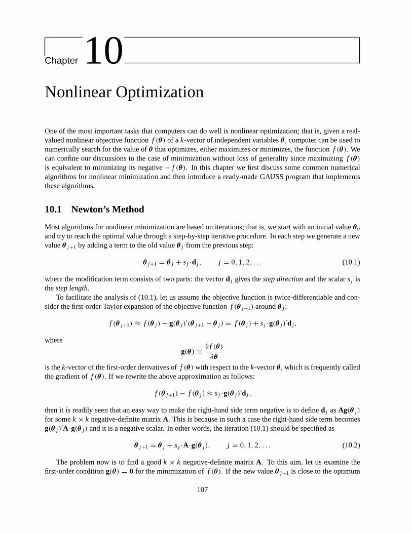
Chapter 10Nonlinear Optimization
One of the most important tasks that computers can do well is nonlinear optimization; that is, given a real-valued nonlinear objective functionf (θθθ) of ak-vector of independent variablesθθθ , computer can be used tonumerically search for the value ofθθθ that optimizes, either maximizes or minimizes, the functionf (θθθ). Wecan confine our discussions to the case of minimization without loss of generality since maximizingf (θθθ)is equivalent to minimizing its negative− f (θθθ). In this chapter we first discuss some common numericalalgorithms for nonlinear minimization and then introduce a ready-made GAUSS program that implementsthese algorithms.
10.1 Newton’s Method
Most algorithms for nonlinear minimization are based on iterations; that is, we start with an initial valueθθθ0
and try to reach the optimal value through a step-by-step iterative procedure. In each step we generate a newvalueθθθ j +1 by adding a term to the old valueθθθ j from the previous step:
θθθ j +1 = θθθ j + sj ·d j , j = 0,1,2, . . . (10.1)
where the modification term consists of two parts: the vectord j gives thestep directionand the scalarsj isthestep length.
To facilitate the analysis of (10.1), let us assume the objective function is twice-differentiable and con-sider the first-order Taylor expansion of the objective functionf (θθθ j +1) aroundθθθ j :
f (θθθ j +1) ≈ f (θθθ j )+ g(θθθ j )′(θθθ j +1 − θθθ j ) = f (θθθ j )+ sj ·g(θθθ j )
′d j ,
where
g(θθθ) ≡∂ f (θθθ)
∂θθθ
is thek-vector of the first-order derivatives off (θθθ) with respect to thek-vectorθθθ , which is frequently calledthe gradient off (θθθ). If we rewrite the above approximation as follows:
f (θθθ j +1)− f (θθθ j ) ≈ sj ·g(θθθ j )′d j ,
then it is readily seen that an easy way to make the right-hand side term negative is to defined j asAg(θθθ j )
for somek × k negative-definite matrixA. This is because in such a case the right-hand side term becomesg(θθθ j )
′A ·g(θθθ j ) and it is a negative scalar. In other words, the iteration (10.1) should be specified as
θθθ j +1 = θθθ j + sj ·A ·g(θθθ j ), j = 0,1,2, . . . (10.2)
The problem now is to find a goodk × k negative-definite matrixA. To this aim, let us examine thefirst-order conditiong(θθθ) = 0 for the minimization of f (θθθ). If the new valueθθθ j +1 is close to the optimum
107

108 CHAPTER 10. NONLINEAR OPTIMIZATION
so that it satisfies the first-order condition, then we have the following first-order Taylor expansion of thegradientg(θθθ j +1) aroundθθθ j :
g(θθθ j +1) ≈ g(θθθ j )+ H(θθθ j )(θθθ j +1 − θθθ j ) = 0, (10.3)
where
H(θθθ) ≡∂g(θθθ)
∂θθθ=∂2 f (θθθ)
∂θθθ∂θθθ ′
is thek×k matrix of the second-order derivatives off (θθθ) with respect to thek-vectorθθθ , which is frequentlycalled Hessian off (θθθ). We note thatH(θθθ j ) is necessarily positive definite whenθθθ j is sufficiently close tothe optimum. From (10.3) we solve forθθθ j +1 = θθθ j − H(θθθ j )
−1g(θθθ j ), which suggests a possible specificationfor (10.2) withsj = 1 andA = −H(θθθ j )
−1. If in (10.2) we allow a general step lengthsj and set the stepdirectiond j as−H(θθθ j )
−1g(θθθ j ), then the iteration formula becomes
θθθ j +1 = θθθ j − sj ·H(θθθ j )−1g(θθθ j ), j = 0,1,2, . . . , (10.4)
which is the basic formula forNewton’s Method. Obviously, to implement Newton’s method, we have torepeatedly compute the gradientg(θθθ j ), the inverted HessianH(θθθ j )
−1, as well as the step lengthsj . We shalldiscuss these computation problems in details shortly.
When applying Newton’s method to solve a nonlinear minimization problem, we iterate the formula(10.4) until convergence is reached. Convergence is usually based on one or more of the following threecriteria:
1. When the absolute value of the difference between successive results‖θθθ j +1 − θθθ j ‖ is smaller than adesired level (such as 10−7);
2. When the absolute value of the difference between successive functional values| f (θθθ j +1)− f (θθθ j )| issmaller than a desired level;
3. When the absolute value of the gradients‖g(θθθ j +1)‖ is smaller than a desired level.
10.1.1 The Computation of Gradients
It is quite often that deriving analytic gradients, i.e., the explicit mathematical expression forg(θθθ), is fairlydifficult and prone to errors, in which cases we need computers to numerically approximate the gradients.Suchnumerical gradientcan be computed based on two operational formulas for derivatives:
1. The forward-difference approximation: the i th element of the gradient vectorg(θθθ j ) is approximatedby
gi (θθθ j ) ≈f (θθθ j + ε ·ιιιi )− f (θθθ j )
ε, i = 1,2, . . . , k,
whereιιιi is ak-dimensional vector of zeros except that thei th element is one, whileε is a very smallscalar, such as 10−8. It should be pointed out that, given the value off (θθθ j ), the calculation of theentirek-dimensional gradient vectorg(θθθ j ) requiresk evaluations of the objective functionf (θθθ j +ε·ιιιi ),for i = 1,2, . . . , k.

10.1. NEWTON’S METHOD 109
2. The central-difference approximation: the i th element of the gradient vectorg(θθθ j ) is approximatedby
gi (θθθ j ) ≈f (θθθ j + ε ·ιιιi )− f (θθθ j − ε ·ιιιi )
2ε, i = 1,2, . . . , k.
Given the value off (θθθ j ), using this formula to calculate the gradient vectorg(θθθ j ) requires 2k eval-uations of the objective functionf (θθθ j + ε · ιιιi ) and f (θθθ j − ε · ιιιi ), for i = 1,2, . . . , k. Hence, thecentral-difference approximation requires two times computation time than the forward-differenceapproximation does. However, the central-difference approximation can only achieve slightly betteraccuracy.
Numerical gradients generally take much longer computation time than evaluating analytic gradients.Thus, it is usually advisable to provide the computer program with the analytic gradients when they areavailable.
10.1.2 The Computation of Hessian
Other than analytically deriving Hessian, we can also apply the same idea for numerical gradients to ap-proximate Hessian. For example, based on the forward-difference approximation we can use the followingformula for the(p,q)th element of the Hessian matrix:
hpq(θθθ j ) ≈f (θθθ j + ε ·ιιιp + ε ·ιιιq)− f (θθθ j + ε ·ιιιp)− f (θθθ j + ε ·ιιιq)+ f (θθθ j )
ε2, (10.5)
for p ≥ q = 1,2, . . . , k. Given the value off (θθθ j ), the calculation of numerical HessianH(θθθ j ), which isa symmetric matrix, requires at leastk(k + 1)/2 evaluations of the objective functionf (θθθ j + ε ·ιιιp + ε ·ιιιq)
as well ask evaluations off (θθθ j + ε ·ιιιp), for p,q = 1,2, . . . , k. Obviously, such computation, as well asthe inversion of the resulting Hessian which is needed in Newton’s formula (10.4), take considerable time.Moreover, the desired level of accuracy is usually hard to maintained with (10.5). If analytic gradientsg(θθθ j )
are available, then we can use a more accurate approximation as follows:
hpq(θθθ j ) ≈gp(θθθ j + ε ·ιιιq)− gp(θθθ j )
ε, (10.6)
for p ≥ q = 1,2, . . . , k. Such calculation requiresk(k + 1)/2 evaluations of the gradient functions and canproduce more accurate results than (10.5).
Since deriving analytic Hessian is generally quite cumbersome and evaluating numerical Hessian isextremely time-consuming, other approaches have been suggested. For example, it is possible to consideran abridged numerical Hessian in which all off-diagonal elements are set to zero:hpq(θθθ j ) = 0, for p 6= q.This special case of Newton’s method, which requires onlyk evaluations of the gradient functions, is referredto as thesteepest descent algorithm. In the next subsection we consider another class of algorithms, the so-calledQuasi-Newton Method, that circumvent almost all Hessian computation.
10.1.3 Quasi-Newton Method
The main idea of Quasi-Newton method is to avoid the tedious evaluations of Hessian and directly modify(or update) the successive inverted Hessian using gradients only. Specifically, we construct the new valueof inverted Hessian at the( j + 1)th step, denoted asH−1
1 , by modifying the previous valueH−1◦
at the j th

110 CHAPTER 10. NONLINEAR OPTIMIZATION
step using gradientsg(θθθ j ) andg(θθθ j +1). To see this, let us first define two vectorsu ≡ −H−1◦
g(θθθ j ) andv ≡ g(θθθ j +1)− g(θθθ j ). Two versions of updating formulas have been proposed.1
1. The Broyden-Fletcher-Goldfarb-Shanno (BFGS) update is:
H−11 = H−1
◦−
1
v′u
(H−1
◦vu′
+ uv′H−1◦
)+
v′H−1◦
v(v′u)2
·uu′+
1
v′u·uu′.
2. The Davidon-Fletcher-Powell (DFP) update is
H−11 = H−1
◦−
1
v′H−1◦
v·H−1
◦vv′H−1
◦+
1
v′u·uu′.
These two formulas can be further modified by multiplying the first three right-hand side terms of theBFGS update and the first two right-hand side terms of the DFP update, respectively, byv′u/v′H−1
◦v. The
resulting formulas are referred to as thescaled BFGS updateand thescaled DFP update, respectively.
10.1.4 Newton’s Method for Maximum Likelihood Estimation
In econometrics applications the need for nonlinear optimization is perhaps most apparent in deriving themaximum likelihood estimator (MLE). Given the samplex1, x2, . . ., xn which are assumed to be inde-pendently distributed with respective density functionsfi (xi |θθθ), whereθθθ is an unknownk-dimensionalparameter and the density functionsfi may not be identical, the MLE ofθθθ is derived by maximizing thelog-likelihood function with respect toθθθ :
ln L(θθθ) =
n∑i =1
ln fi (xi |θθθ).
This maximization is equivalent to minimizing the negative log-likelihood function− ln L(θθθ).Since the second-order derivative of the log-density function∂2 ln fi (xi |θθθ)/∂θθθ∂θθθ
′, as a function of therandom variablexi , is a random variable, the law of large numbers implies that, under certain regularityconditions, we have
1
n
∂2 ln L(θθθ)
∂θθθ∂θθθ ′−
1
nE
[∂2 ln L(θθθ)
∂θθθ∂θθθ ′
]=
1
n
n∑i =1
{∂2 ln fi (xi |θθθ)
∂θθθ∂θθθ ′− E
[∂2 ln fi (xi |θθθ)
∂θθθ∂θθθ ′
]}p
−→ 0,
as the sample sizen goes to infinity. Consequently, the Hessian matrix in (10.4), which in the presentcase is−∂2 ln L(θθθ)/∂θθθ∂θθθ ′, can be approximated by its expectation (which in the MLE theory is called theinformation matrix):
H(θθθ j ) ≈ −E
[∂2 ln L(θθθ j )
∂θθθ∂θθθ ′
]. (10.7)
Newton’s method with such an approximate Hessian is called themethod of scoring. Its usefulness lies onthe fact that taking expectation usually helps simplify the expression of Hessian.
1Both of these formulas forH−11 satisfy the equalityH−1
1 v = u or, equivalently,g(θθθ j ) − g(θθθ j +1) = H1H−1◦ g(θθθ j ). This
condition can be motivated by the following first-order Taylor expansion of gradientg(θθθ j ) aroundθθθ j +1: g(θθθ j ) = g(θθθ j +1) +
H1(θθθ j − θθθ j +1), while from (10.4) we haveθθθ j − θθθ j +1 = H−1◦ g(θθθ j ) (where the step lengthsj is set to one).

10.2. A GAUSS PROGRAM FOR NONLINEAR MINIMIZATION: NLOPT 111
There is one more approximation to the Hessian matrix of the log-likelihood function that is based onthe equality
−E
[∂2 ln fi (xi |θθθ)
∂θθθ∂θθθ ′
]= E
[∂ ln fi (xi |θθθ)
∂θθθ·∂ ln fi (xi |θθθ)
∂θθθ ′
].
Again, the law of large numbers implies that, under certain regularity conditions, we have
−1
n
∂2 ln L(θθθ)
∂θθθ∂θθθ ′−
1
n
n∑i =1
∂ ln fi (xi |θθθ)
∂θθθ·∂ ln fi (xi |θθθ)
∂θθθ ′
p−→ 0,
as the sample sizen goes to infinity. As a result, we have another approximation to the Hessian matrix:
H(θθθ j ) ≈
n∑i =1
∂ ln fi (xi |θθθ j )
∂θθθ·∂ ln fi (xi |θθθ j )
∂θθθ ′. (10.8)
Newton’s method with such an approximate Hessian is referred to as the Berndt-Hall-Hall-Hausman (BHHH)method.
Asymptotic Standard Errors for MLE: The asymptotic theory for the MLE indicates that for the MLEθθθ , we have
θθθA∼ N
(θθθ,
{−E
[∂2 ln L(θθθ)
∂θθθ∂θθθ ′
]}−1).
Hence, if we apply the method of scoring or the BHHH method, then the inverse of the Hessian matrix (10.7)or (10.8) after convergence is reached can be readily used as an approximate variance-covariance matrix forthe MLE (so that the square roots of its diagonal elements are standard errors). In other words, no furthercomputation is needed to obtain the standard errors of the MLE.
Finally, we should note that when quasi-Newton method is used to derive the MLE, the inverse of theapproximate Hessian, constructed either by the BFGS formula or by the DFP formula,cannotbe usedas an approximate variance-covariance matrix for the MLE. Hence, after convergence is arrived, it is stillnecessary to go one step further to numerically evaluate Hessian based on (10.5), (10.6), (10.7), or (10.8).
10.1.5 The Computation of the Step Length
Once the gradientg(θθθ j ) and HessianH(θθθ j ) (or its approximation) for the new step direction in (10.4) areobtained, the value of the objective function can be viewed as a function of the step lengthsj only. Thedetermination ofsj then becomes a one-dimensional minimization problem (which is sometimes called aline search problem). There are two popular line search methods: thebacktrack algorithmand thegoldensearch algorithm. Each method involves a particular trial-and-error search scheme. Here, without goinginto details, we only point out that the backtrack algorithm requires less computation while the goldensearch algorithm is more effective in finding a better step length. Finally, we note that settingsj = 1indiscriminately usually worsens instead improves the value of the objective function.
10.2 A GAUSS Program for Nonlinear Minimization: NLOPT
NLOPT is a self-contained GAUSS procedure for nonlinear minimization. Once the procedure is properlyinstalled, all a user needs to do is to write the (differentiable) objective function as a function of a vector ofindependent variables in the format of GAUSS procedure.

112 CHAPTER 10. NONLINEAR OPTIMIZATION
The source codes of the procedureNLOPT are stored in the file ‘NLOPT.GCG’. To use it, simply add thecommand ‘use nlopt;’ at the beginning of the file where you type your program and place the ‘NLOPT.GCG’file in the same subdirectory as your program file.
Consider a simple example of minimizing the following function of a single variable:
f (θ) = −3θ2e−θ3.
To solve this problem, we write a short program to call the procedureNLOPT :
1 new;2 use nlopt;3
4 proc ofn(t);5 local f;6 f = -3*(tˆ2)*exp(-tˆ3);7 retp(f);8 endp;9
10 start = 1;11
12 {parout,vof,gout,retcode} = nlopt(&ofn,start);13
14 end;
The first part of the program after the ‘use nlopt;’ command is the definition of procedure ‘ofn’ whichtakes one input ‘t’ and yields one output ‘f’. It is the place where we write the definition of the objectivefunction f (θθθ). The input is of course the vector of independent variables (i.e.,θθθ ) and the output is the valueof the objective function (i.e.,f ). In the above example there is only one independent variable and the valueof the objective function is also a scalar.
It should be pointed out that in cases where there are more than one independent variable in the vectorθθθ ,an important consideration in setting up the definition of the ‘ofn’ procedure is that the values of independentvariables should be made about the same magnitude. For example, suppose we are considering a functionof two independent variablesf (θ1, θ2). If the optimal value ofθ1 is 12345.67890 while that ofθ2 is 0.9876,then we should redefine the function asf (10000θ1, θ2) so that the function will be minimized with thesolution 1.234567890 and 0.9876 forθ1 andθ2, respectively. Doing this helps smoothing the convergenceof the iterations and increasing the accuracy of the solution.
Immediately after the procedure definition is the specification of the column vector ‘start’ (which is ascalar in the above example). This vector contains the initial values of the independent variableθθθ , which areneeded to start Newton’s iteration formula (10.4). Initial values are usually set by the user subjectively.
The procedureNLOPT is called by the ‘nlopt’ command which takes two inputs and produces fouroutputs. The two inputs are respectively the procedure ‘ofn’ and the vector ‘start’ which have just beendefined. Among the four outputs, the column vector ‘parout’ contains the solution; the scalar ‘vof’ givesthe minimized function value evaluated at ‘parout’; the column vector ‘gout’ is the gradient evaluated at‘parout’; and ‘retcode’ is a returned code indicating the program execution status. Returned codes areexplained in Table 1.
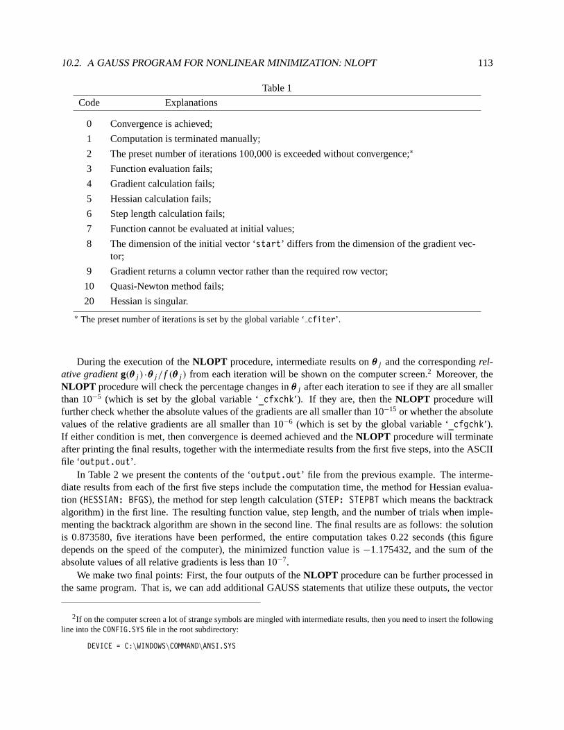
10.2. A GAUSS PROGRAM FOR NONLINEAR MINIMIZATION: NLOPT 113
Table 1
Code Explanations
0 Convergence is achieved;
1 Computation is terminated manually;
2 The preset number of iterations 100,000 is exceeded without convergence;∗
3 Function evaluation fails;
4 Gradient calculation fails;
5 Hessian calculation fails;
6 Step length calculation fails;
7 Function cannot be evaluated at initial values;
8 The dimension of the initial vector ‘start’ differs from the dimension of the gradient vec-tor;
9 Gradient returns a column vector rather than the required row vector;
10 Quasi-Newton method fails;
20 Hessian is singular.
∗ The preset number of iterations is set by the global variable ‘cfiter’.
During the execution of theNLOPT procedure, intermediate results onθθθ j and the correspondingrel-ative gradientg(θθθ j ) ·θθθ j / f (θθθ j ) from each iteration will be shown on the computer screen.2 Moreover, theNLOPT procedure will check the percentage changes inθθθ j after each iteration to see if they are all smallerthan 10−5 (which is set by the global variable ‘_cfxchk’). If they are, then theNLOPT procedure willfurther check whether the absolute values of the gradients are all smaller than 10−15 or whether the absolutevalues of the relative gradients are all smaller than 10−6 (which is set by the global variable ‘_cfgchk’).If either condition is met, then convergence is deemed achieved and theNLOPT procedure will terminateafter printing the final results, together with the intermediate results from the first five steps, into the ASCIIfile ‘output.out’.
In Table 2 we present the contents of the ‘output.out’ file from the previous example. The interme-diate results from each of the first five steps include the computation time, the method for Hessian evalua-tion (HESSIAN: BFGS), the method for step length calculation (STEP: STEPBT which means the backtrackalgorithm) in the first line. The resulting function value, step length, and the number of trials when imple-menting the backtrack algorithm are shown in the second line. The final results are as follows: the solutionis 0.873580, five iterations have been performed, the entire computation takes 0.22 seconds (this figuredepends on the speed of the computer), the minimized function value is−1.175432, and the sum of theabsolute values of all relative gradients is less than 10−7.
We make two final points: First, the four outputs of theNLOPT procedure can be further processed inthe same program. That is, we can add additional GAUSS statements that utilize these outputs, the vector
2If on the computer screen a lot of strange symbols are mingled with intermediate results, then you need to insert the followingline into theCONFIG.SYS file in the root subdirectory:
DEVICE = C:\WINDOWS\COMMAND\ANSI.SYS

114 CHAPTER 10. NONLINEAR OPTIMIZATION
‘parout’ in particular, after the ‘nlopt’ command. Secondly, we should understand there is no guaranteethat the result we obtain from theNLOPT procedure is always theglobalminimum of the objective function.To guard against the possibility of getting a local minimum, all we can do is to try different starting valuesand see whether we always reach the same solution. If there are more than one solution, we wish to get theglobal one among those local solutions.
10.2.1 Changing Options
In the previous example, theNLOPT procedure is executed in its standard form. The computation methodsused there consist of the forward-difference approximation for numerical gradients, the BFGS version ofquasi-Newton method for Hessian updates (where the identity matrix is used as the initial value for Hessian),and the backtrack algorithm for the step length. Each of these specifications can be changed and manyalternative options are available. To make changes, we simply assign one or more of the following globalvariables (switches) with different values before calling theNLOPT procedure:3
1. The global variable ‘_cfgdmd’ determines the algorithm for calculating numerical gradients. Possiblevalues are:
0: The central-difference approximation;
1: The forward-difference approximation (the default);
2: The Richardson extrapolation method.
2. The global variable ‘_cfhsmd’ determines Hessian updating algorithm. Possible values are:
1: Quasi-Newton method – the BFGS algorithm (the default);
2: Quasi-Newton method – the scaled BFGS algorithm;
3: Quasi-Newton method – the DFP algorithm;
4: Quasi-Newton method – the scaled DFP algorithm;
5: Newton’s method with numerical/analytic Hessian (Hessian is evaluated either numerically bythe forward-difference approximation or analytically by user’s definition);
6: The steepest descent algorithm;
3. The global variable ‘_cfstep’ determines the algorithm for calculating the step length. Possiblevalues are:
1: The step length is fixed at one;
2: The backtrack method (the default);
3: The golden search method;
4: The Brent method.
3Besides the various computation methods for numerical gradients, Hessian, and step length that have been described in theprevious section, we note that there is one more method for numerical gradients: the Richardson extrapolation method, and onemore for the step length: the Brent method. However, both methods are rarely used and will note be discussed here.

10.2. A GAUSS PROGRAM FOR NONLINEAR MINIMIZATION: NLOPT 115
Table 2: The Contents of theoutput.out File
1 *************************************************************************2 ITER:1 TIME:0.00 SEC. HESSIAN: BFGS STEP: STEPBT3 FUNCTION: -1.103638 STEP LENGTH: 0.000 BACKSTEPS: 04 *************************************************************************5 1 1.00000 1.0000006 *************************************************************************7 ITER:2 TIME:0.00 SEC. HESSIAN: BFGS STEP: STEPBT8 FUNCTION: -1.106689 STEP LENGTH: 0.250 BACKSTEPS: 19 *************************************************************************
10 1 0.75000 0.73437511 *************************************************************************12 ITER:3 TIME:0.00 SEC. HESSIAN: BFGS STEP: STEPBT13 FUNCTION: -1.175431 STEP LENGTH: 1.000 BACKSTEPS: 014 *************************************************************************15 1 0.87386 0.00189816 *************************************************************************17 ITER:4 TIME:0.00 SEC. HESSIAN: BFGS STEP: STEPBT18 FUNCTION: -1.175432 STEP LENGTH: 1.000 BACKSTEPS: 019 *************************************************************************20 1 0.87357 0.00010221 *************************************************************************22 ITER:5 TIME:0.00 SEC. HESSIAN: BFGS STEP: STEPBT23 FUNCTION: -1.175432 STEP LENGTH: 1.000 BACKSTEPS: 024 *************************************************************************25 1 0.87358 0.00000026 *************************************************************************27
28 *************************************************************************29 PARAMETER ESTIMATE PARAMETER ESTIMATE30 *************************************************************************31 PAR. 01 0.87358032 *************************************************************************33
34 NORMAL CONVERGENCE IS ACHIEVED35
36 FINAL RESULTS37 *************************************************38 ITERATION: 539 TIME: 0.22 SECONDS40 FUNCTION: -1.17543241 REL. GRAD.: 0.000000042 *************************************************
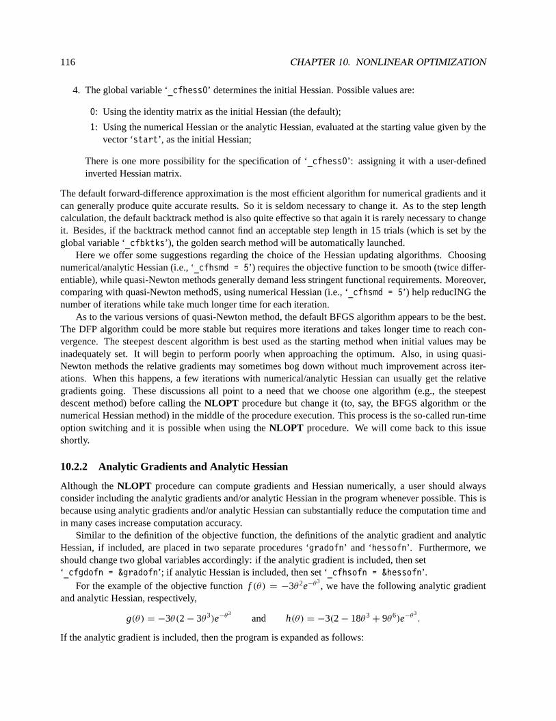
116 CHAPTER 10. NONLINEAR OPTIMIZATION
4. The global variable ‘_cfhess0’ determines the initial Hessian. Possible values are:
0: Using the identity matrix as the initial Hessian (the default);
1: Using the numerical Hessian or the analytic Hessian, evaluated at the starting value given by thevector ‘start’, as the initial Hessian;
There is one more possibility for the specification of ‘_cfhess0’: assigning it with a user-definedinverted Hessian matrix.
The default forward-difference approximation is the most efficient algorithm for numerical gradients and itcan generally produce quite accurate results. So it is seldom necessary to change it. As to the step lengthcalculation, the default backtrack method is also quite effective so that again it is rarely necessary to changeit. Besides, if the backtrack method cannot find an acceptable step length in 15 trials (which is set by theglobal variable ‘_cfbktks’), the golden search method will be automatically launched.
Here we offer some suggestions regarding the choice of the Hessian updating algorithms. Choosingnumerical/analytic Hessian (i.e., ‘_cfhsmd = 5’) requires the objective function to be smooth (twice differ-entiable), while quasi-Newton methods generally demand less stringent functional requirements. Moreover,comparing with quasi-Newton methodS, using numerical Hessian (i.e., ‘_cfhsmd = 5’) help reducING thenumber of iterations while take much longer time for each iteration.
As to the various versions of quasi-Newton method, the default BFGS algorithm appears to be the best.The DFP algorithm could be more stable but requires more iterations and takes longer time to reach con-vergence. The steepest descent algorithm is best used as the starting method when initial values may beinadequately set. It will begin to perform poorly when approaching the optimum. Also, in using quasi-Newton methods the relative gradients may sometimes bog down without much improvement across iter-ations. When this happens, a few iterations with numerical/analytic Hessian can usually get the relativegradients going. These discussions all point to a need that we choose one algorithm (e.g., the steepestdescent method) before calling theNLOPT procedure but change it (to, say, the BFGS algorithm or thenumerical Hessian method) in the middle of the procedure execution. This process is the so-called run-timeoption switching and it is possible when using theNLOPT procedure. We will come back to this issueshortly.
10.2.2 Analytic Gradients and Analytic Hessian
Although theNLOPT procedure can compute gradients and Hessian numerically, a user should alwaysconsider including the analytic gradients and/or analytic Hessian in the program whenever possible. This isbecause using analytic gradients and/or analytic Hessian can substantially reduce the computation time andin many cases increase computation accuracy.
Similar to the definition of the objective function, the definitions of the analytic gradient and analyticHessian, if included, are placed in two separate procedures ‘gradofn’ and ‘hessofn’. Furthermore, weshould change two global variables accordingly: if the analytic gradient is included, then set‘_cfgdofn = &gradofn’; if analytic Hessian is included, then set ‘_cfhsofn = &hessofn’.
For the example of the objective functionf (θ) = −3θ2e−θ3, we have the following analytic gradient
and analytic Hessian, respectively,
g(θ) = −3θ(2 − 3θ3)e−θ3and h(θ) = −3(2 − 18θ3
+ 9θ6)e−θ3.
If the analytic gradient is included, then the program is expanded as follows:
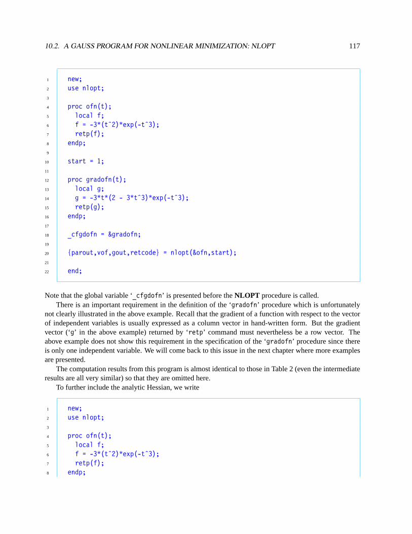
10.2. A GAUSS PROGRAM FOR NONLINEAR MINIMIZATION: NLOPT 117
1 new;2 use nlopt;3
4 proc ofn(t);5 local f;6 f = -3*(tˆ2)*exp(-tˆ3);7 retp(f);8 endp;9
10 start = 1;11
12 proc gradofn(t);13 local g;14 g = -3*t*(2 - 3*tˆ3)*exp(-tˆ3);15 retp(g);16 endp;17
18 _cfgdofn = &gradofn;19
20 {parout,vof,gout,retcode} = nlopt(&ofn,start);21
22 end;
Note that the global variable ‘_cfgdofn’ is presented before theNLOPT procedure is called.There is an important requirement in the definition of the ‘gradofn’ procedure which is unfortunately
not clearly illustrated in the above example. Recall that the gradient of a function with respect to the vectorof independent variables is usually expressed as a column vector in hand-written form. But the gradientvector (‘g’ in the above example) returned by ‘retp’ command must nevertheless be a row vector. Theabove example does not show this requirement in the specification of the ‘gradofn’ procedure since thereis only one independent variable. We will come back to this issue in the next chapter where more examplesare presented.
The computation results from this program is almost identical to those in Table 2 (even the intermediateresults are all very similar) so that they are omitted here.
To further include the analytic Hessian, we write
1 new;2 use nlopt;3
4 proc ofn(t);5 local f;6 f = -3*(tˆ2)*exp(-tˆ3);7 retp(f);8 endp;

118 CHAPTER 10. NONLINEAR OPTIMIZATION
9
10 start = 1;11
12 proc gradofn(t);13 local g;14 g = -3*t*(2 - 3*tˆ3)*exp(-tˆ3);15 retp(g);16 endp;17
18 _cfgdofn = &gradofn;19
20 proc hessofn(t);21 local g;22 g = -3*(2- 18*tˆ3 + 9*tˆ6)*exp(-tˆ3);23 retp(g);24 endp;25
26 _cfhsofn = &hessofn;27 _cfhsmd = 5;28
29 {parout,vof,gout,retcode} = nlopt(&ofn,start);30
31 end;
In addition to the procedure ‘_gradofn’ and the global variable ‘_cfgdofn’, we present the procedure‘_hessofn’ and the global variable ‘_cfhsofn’ before calling theNLOPT procedure. We also change thevalue of the global variable ‘_cfhsmd’ in order to pick Newton’s method so that the analytic Hessian definedin the ‘_hessofn’ procedure can be fully utilized. The output file are shown in Table 3. The final resultsare the same as in Table 2 but the intermediate results are not. In particular, the function values, the variablevalues, and the corresponding relative gradients in steps 3 and 4 are quite different.
Deriving analytic gradients and including them as a part of the program are strongly encouraged. Butin many cases trying to do the same for analytic Hessian can be much more difficult, if not completely in-tractable. So the best strategy in most applications appears to be including analytic gradients in the programand then applying one of the quasi-Newton methods that use gradients to approximate the inverted Hessian.
This strategy is also applicable to most MLE applications. As mentioned in subsection 10.1.4, in additionto the MLE themselves we often need to compute the corresponding asymptotic variance-covariance matrix,which can be approximated by the inverted Hessian. But the approximated inverted Hessian generated by thequasi-Newton method cannot be used for this purpose. So it is necessary to go one step further to evaluateHessian numerically using the formula (10.6). To do this, we simply change the value of the global variable‘_cfmlese’ to 1 by the following statement before calling theNLOPT procedure:
1 _cfmlese = 1;
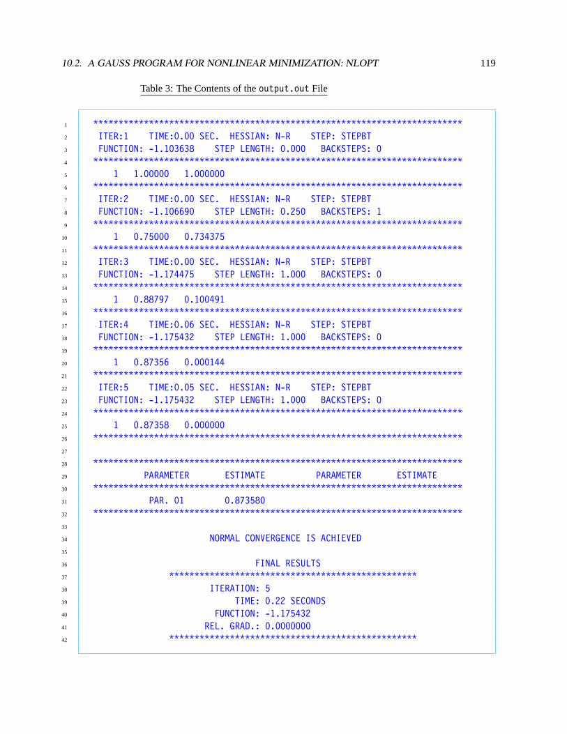
10.2. A GAUSS PROGRAM FOR NONLINEAR MINIMIZATION: NLOPT 119
Table 3: The Contents of theoutput.out File
1 *************************************************************************2 ITER:1 TIME:0.00 SEC. HESSIAN: N-R STEP: STEPBT3 FUNCTION: -1.103638 STEP LENGTH: 0.000 BACKSTEPS: 04 *************************************************************************5 1 1.00000 1.0000006 *************************************************************************7 ITER:2 TIME:0.00 SEC. HESSIAN: N-R STEP: STEPBT8 FUNCTION: -1.106690 STEP LENGTH: 0.250 BACKSTEPS: 19 *************************************************************************
10 1 0.75000 0.73437511 *************************************************************************12 ITER:3 TIME:0.00 SEC. HESSIAN: N-R STEP: STEPBT13 FUNCTION: -1.174475 STEP LENGTH: 1.000 BACKSTEPS: 014 *************************************************************************15 1 0.88797 0.10049116 *************************************************************************17 ITER:4 TIME:0.06 SEC. HESSIAN: N-R STEP: STEPBT18 FUNCTION: -1.175432 STEP LENGTH: 1.000 BACKSTEPS: 019 *************************************************************************20 1 0.87356 0.00014421 *************************************************************************22 ITER:5 TIME:0.05 SEC. HESSIAN: N-R STEP: STEPBT23 FUNCTION: -1.175432 STEP LENGTH: 1.000 BACKSTEPS: 024 *************************************************************************25 1 0.87358 0.00000026 *************************************************************************27
28 *************************************************************************29 PARAMETER ESTIMATE PARAMETER ESTIMATE30 *************************************************************************31 PAR. 01 0.87358032 *************************************************************************33
34 NORMAL CONVERGENCE IS ACHIEVED35
36 FINAL RESULTS37 *************************************************38 ITERATION: 539 TIME: 0.22 SECONDS40 FUNCTION: -1.17543241 REL. GRAD.: 0.000000042 *************************************************

120 CHAPTER 10. NONLINEAR OPTIMIZATION
The resulting inverse of the numerical Hessian4 will go to the the global variable ‘_cfhess1’ which can thenbe further processed. For example, after setting the global variable ‘_cfmlese’ to 1 and calling theNLOPTprocedure to calculate the MLE, the standard errors of the resulting MLE can be computed (and assigned tovariable ‘se’) by the following statement:
1 se = sqrt(diag(_cfhess1));
10.2.3 Imposing Restrictions
In this subsection we explain how to impose some common restrictions on the value of an independentvariable, say,θ1 when using theNLOPT procedure to minimize the objective functionf (θ1, θθθ2), whereθθθ2
is the subvector of other variables. We consider three types of restrictions:5
1. θ1 ∈ (0, ∞);
2. θ1 ∈ (0, 1);
3. θ1 ∈ (−1, 1).
The approach we adopt here is based on a transformation of the original variable under restriction to someunrestricted new variable. The idea is to change the restricted minimization problem to an unrestricted oneso that we can apply theNLOPT procedure as usual.
In the first case where the value of the independent variableθ1 is restricted to be positive, we considerthe following one-to-one transformation from the original variableθ1 to the new oneδ:
θ1 = k(δ) ≡ eδ ∈ (0, ∞). (10.9)
We note that the new variableδ = ln θ1 is completely unrestricted. In the second case where the valueof the independent variableθ1 is restricted to be between 0 and 1, we consider the following one-to-onetransformation:
θ1 = k′(δ) ≡1
e−δ + 1∈ (0, 1), (10.10)
whereδ = ln[θ1/(1 − θ1)] can assume any value and is therefore unrestricted. In the third case wherethe value of the independent variableθ1 is restricted to be between−1 and 1, we consider the followingone-to-one transformation:
θ1 = k′′(δ) ≡eδ − 1
eδ + 1∈ (−1, 1), (10.11)
whereδ = ln[(1 + θ1)/(1 − θ1)] is necessarily unrestricted. We note that in each of these three cases, wecan rewrite the objective functionf (θ1, θθθ1) of the original variable as a function of the unrestricted newvariable. For example, for the first case we havef (δ, θθθ2) ≡ f
[k(δ), θθθ2
].
4If the analytic gradient is not included in the program, then the formula (10.5) will be used. In such a case the computation willtake substantially more time and generate much less accurate results.
5The upper bound of the second type of restriction as well as the absolute value of the two bounds of the third type of restrictioncan be extended from 1 to any positive number.
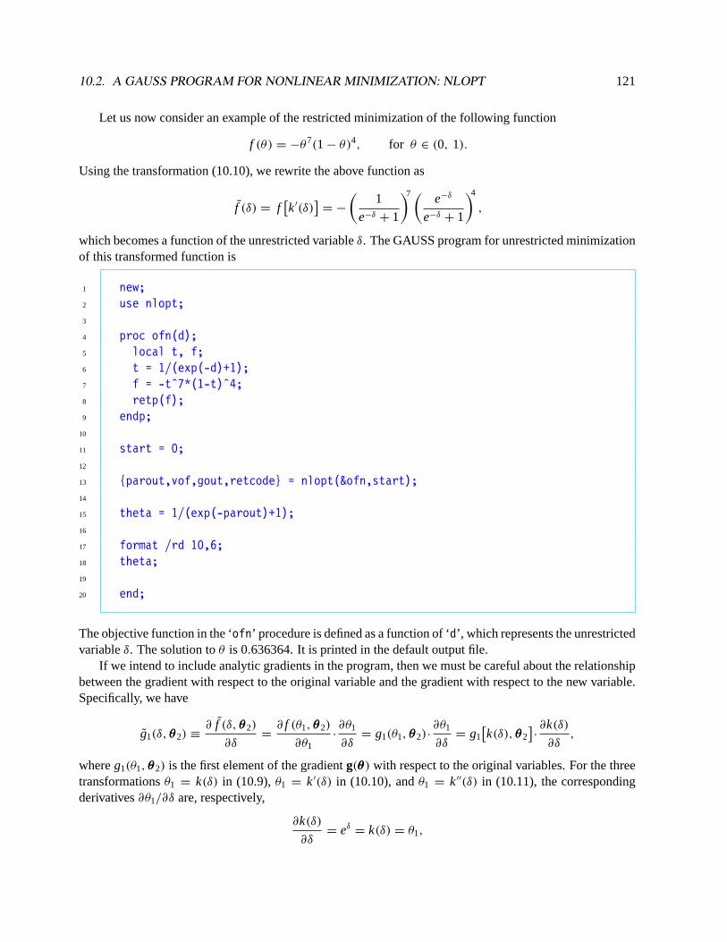
10.2. A GAUSS PROGRAM FOR NONLINEAR MINIMIZATION: NLOPT 121
Let us now consider an example of the restricted minimization of the following function
f (θ) = −θ7(1 − θ)4, for θ ∈ (0, 1).
Using the transformation (10.10), we rewrite the above function as
f (δ) = f[k′(δ)
]= −
(1
e−δ + 1
)7( e−δ
e−δ + 1
)4
,
which becomes a function of the unrestricted variableδ. The GAUSS program for unrestricted minimizationof this transformed function is
1 new;2 use nlopt;3
4 proc ofn(d);5 local t, f;6 t = 1/(exp(-d)+1);7 f = -tˆ7*(1-t)ˆ4;8 retp(f);9 endp;
10
11 start = 0;12
13 {parout,vof,gout,retcode} = nlopt(&ofn,start);14
15 theta = 1/(exp(-parout)+1);16
17 format /rd 10,6;18 theta;19
20 end;
The objective function in the ‘ofn’ procedure is defined as a function of ‘d’, which represents the unrestrictedvariableδ. The solution toθ is 0.636364. It is printed in the default output file.
If we intend to include analytic gradients in the program, then we must be careful about the relationshipbetween the gradient with respect to the original variable and the gradient with respect to the new variable.Specifically, we have
g1(δ, θθθ2) ≡∂ f (δ, θθθ2)
∂δ=∂ f (θ1, θθθ2)
∂θ1·∂θ1
∂δ= g1(θ1, θθθ2)·
∂θ1
∂δ= g1
[k(δ), θθθ2
]·∂k(δ)
∂δ,
whereg1(θ1, θθθ2) is the first element of the gradientg(θθθ) with respect to the original variables. For the threetransformationsθ1 = k(δ) in (10.9),θ1 = k′(δ) in (10.10), andθ1 = k′′(δ) in (10.11), the correspondingderivatives∂θ1/∂δ are, respectively,
∂k(δ)
∂δ= eδ = k(δ) = θ1,

122 CHAPTER 10. NONLINEAR OPTIMIZATION
∂k′(δ)
∂δ=
1
e−δ + 1
(1 −
1
e−δ + 1
)= k′(δ)
[1 − k′(δ)
]= θ1(1 − θ1),
and
∂k′′(δ)
∂δ=
1
2
(1 +
eδ − 1
eδ + 1
)(1 −
eδ − 1
eδ + 1
)=
1
2
[1 + k′′(δ)
][1 − k′′(δ)
]=
1
2(1 + θ1)(1 − θ1).
In the above example, the gradient with respect to the original variable is
g(θ) = −θ6(1 − θ)3(7 − 11θ),
while the gradient with respect to the new variable is
g(δ) = g[k′(δ)
]·∂k′(δ)
∂δ= −θ6(1 − θ)3(7 − 11θ)·θ(1 − θ) = −θ7(1 − θ)4(7 − 11θ)
= −
(1
e−δ + 1
)7(1 −
1
e−δ + 1
)4(7 − 11·
1
e−δ + 1
)If we include the analytic gradient in the program, then we have
1 new;2 use nlopt;3
4 proc ofn(d);5 local t, f;6 t = 1/(exp(-d)+1);7 f = -tˆ7*(1-t)ˆ4;8 retp(f);9 endp;
10
11 start = 0;12
13 proc gradofn(d);14 local t, g;15 t = 1/(exp(-d)+1);16 g = -tˆ7*((1-t)ˆ4)*(7-11*t);17 retp(g);18 endp;19
20 _cfgdofn = &gradofn;21
22 {parout,vof,gout,retcode} = nlopt(&ofn,start);23
24 theta = 1/(exp(-parout)+1);25
26 format /rd 10,6;

10.2. A GAUSS PROGRAM FOR NONLINEAR MINIMIZATION: NLOPT 123
27 theta;28
29 end;
If we also want to include analytic Hessian in the program, then we must first examine the relationshipbetween the Hessian with respect to the original variable and the Hessian with respect to the new variable.These analyses, which are somewhat cumbersome, will be omitted here.
10.2.4 Additional Options
The file name of the output file can be changed from the default ‘output.out’ to, say, ‘trial.1st’ by thefollowing standard GAUSS command for ASCII output:
1 output file = trial.1st reset;
The printing of the computation results can be controlled by the global variable ‘__output’, whose possiblevalues are
0: Only the final results will go to screen and the output file;
1: Iteration number, time, function and relative gradient values, step length, step methods, Hessianalgorithm, and the final results will go to both the screen and the output file;
2: Besides those of the choice 1, all intermediate variable values and the corresponding relative gra-dients will go to the screen; those from the first five iterations will also go to the output file (thedefault).
If we want to specify the variable names in the final printouts (the default are ‘PAR. 01’, ‘ PAR. 02’,‘PAR. 03’, . . .), we can assign the global variable ‘_cfvarnm’ with a character vector of the desired variablenames.
If for some reasons the program is terminated before reaching convergence, then it may be useful toretain those intermediate variable values and the corresponding inverted Hessian right before the programstops. Inspecting these intermediate results might help determine why the program is abnormally termi-nated. They can also be used as the initial values (i.e., by assigning them to the global variables ‘start’and ‘_cfhess0’, respectively) to restart the program. TheNLOPT procedure always keeps the latest in-termediate variable values and the corresponding inverted Hessian in the global variables ‘_cfintvv’ and‘_cfhess1’, respectively.
10.2.5 Run-Time Option Switching
Many options can be changed while theNLOPT procedure is running. In Table 4 we list the key commandsfor all run-time option switching. TheNLOPT procedure will respond to these key commands at the endof each iteration. For example, no matter which algorithm for step length calculation is set in the program,

124 CHAPTER 10. NONLINEAR OPTIMIZATION
Table 4. Run-Time Option Switching
Key Effect Explanation
1. ALT 1 Set_cfhsmd = 1 Quasi-Newton method – the BFGS update2. ALT 2 Set_cfhsmd = 2 Quasi-Newton method – the scaled BFGS update3. ALT 3 Set_cfhsmd = 3 Quasi-Newton method – the DFP update4. ALT 4 Set_cfhsmd = 4 Quasi-Newton method – the scaled DFP update5. ALT 5 Set_cfhsmd = 5 Numerical/analytic Hessian6. ALT 6 Set_cfhsmd = 6 The steepest descent method
7. SFT 1 Set_cfstep = 1 Step length fixed at 18. SFT 2 Set_cfstep = 2 The backtrack method9. SFT 3 Set_cfstep = 3 The golden search method
10. SFT 4 Set_cfstep = 4 The Brent method
11. 0 Set__output = 0 Output control: option 012. 1 Set__output = 1 Output control: option 113. 2 Set__output = 2 Output control: option 2
14. ALT C Force Convergence Exit program immediately15. ALT G Change_cfgdmd Change gradient method16. ALT N Change_cfmlese Whether to evaluate final inverted Hessian17. ALT V Change_cfgchk Change gradient convergence criterion18. ALT M Set_cfbktks Change the number of trials allowed in step length search19. ALT I Compute Hessian immediately20. ALT E Edit variable values∗
21. <PgUp> Print the previous 54 parameters∗∗
22. <PgDn> Print the next 54 parameters∗∗
∗ Pressing ‘ALT E’ brings the program into an interactive mode under which we can alter variable values.∗∗ When the number of variables is greater than 54 so that not all intermediate results can be shown on onescreen, then using ‘<PgUp>’ and ‘<PgDn>’ keys can control which 54 variables to show.
pressing ‘SFT 3’ (i.e., pressing ‘Shift’ and ‘3’ simultaneously) while the program is running switches thealgorithm to the golden search method.6 7
Running NLOPT Recursively: The procedures ‘OFN’, ‘ GRADOFN’, ‘ HESSOFN’ themselves can call theNLOPT procedure. The number of nested levels is limited only by the amount of computer memory. Each
6If the program is taking too many iterations using the default backtrack method, trying golden search for a few iterations thisway (and then pressing ‘SFT 2’ to switch back to the backtrack method) may help speed up convergence.
7When we press ‘ALT E’ and enter into an interactive modeare, then the top two lines on the screen will list current variablevalues one at a time that is ready for changes. We can then do one of the following: (1) press ‘CURSOR UP’ and ‘CURSOR DOWN’ tomove along the variable list back and forth; (2) Press ‘ENTER’ to select the variable for editing, type the new value, and then press‘ENTER’; (3) Press ‘Q’ or ‘ q’ to quit. As soon as a variable value is changed, Hessian will be reset to the identity matrix if any of thequasi-Newton methods is being used.

10.2. A GAUSS PROGRAM FOR NONLINEAR MINIMIZATION: NLOPT 125
level contains its own set of global variables. However, the run-time option switches can be used only at onelevel of theNLOPT procedure, where the value of the corresponding global variable ‘_cfrtos’ should be1 (the default) while those for other levels should all be 0.
10.2.6 Global Variable List
We summarize the global variables used by theNLOPT procedure in Tables 5 and 6. Each of these globalvariables controls one aspect of the procedure and can be changed before calling theNLOPT procedure.Those in Table 5 are the ones that have been discussed in the previous subsections.
There are still a few control variables that are less important and have not yet been discussed. They arepresented in Table 6.
The global variable ‘_cfusrch’ needs some explanations. It allows us to set the step length manuallyduring the run-time. Setting the value of the global variable ‘_cfusrch’ to 1 before calling theNLOPTprocedure causes the program to enter into an interactive mode if all methods for calculating step length fail.Under such an interactive mode, lines 6 to lines 25 on the screen show the initial function value as well asa new function value with a step length of 1. A number 0.1 listed as ‘Stepsize Change’ will also appear.This is a value to be used as an increment for changing the value of current step length. We can do one ofthe following:
• Press ‘CURSOR UP’ to raise the ‘Stepsize Change’ 10 times;
• Press ‘CURSOR DOWN’ to reduce the ‘Stepsize Change’ 10 times;
• Press ‘+’ to increase the step length by the amount of ‘Stepsize Change’ and to recompute thefunction value;
• Press ‘-’ to decrease the step length by the amount of ‘Stepsize Change’ and to recompute thefunction value.
After pressing ‘+’ or ‘ -’, a new function value will be computed based on the new step length. The differ-ence between this new function value and the initial one, together with the corresponding new step length,will be listed in light white color if the new function value is lower than the initial one, and in dark graycolor otherwise. Step lengths can be repeatedly tried and 20 trial results will be shown on the screen simul-taneously for comparisons. When a step length with a lower function value occurs (i.e. a light white colorappears on the screen), press ‘Q’ to exit the interactive mode. The last step length used will be accepted bytheNLOPT procedure as a new step length and the iteration will continue.

126 CHAPTER 10. NONLINEAR OPTIMIZATION
Table 5. The List of Global Variables
Variable Default Explanation
1. _cfgdmd 1 Switch for numerical gradient evaluation algorithms. It can be changedduring the run time by pressing ‘ALT G’.
2. _cfhsmd 1 Switch for Hessian evaluation algorithms. It can be changed during the runtime by pressing ‘ALT 1 -- 5’.
3. _cfstep 2 Switch for step length evaluation algorithms. It can be changed during therun time by pressing ‘SFT 1 -- 4’.
4. _cfgdofn 0 Switch for analytic gradients.
5. _cfhsofn 0 Switch for analytic Hessian.
6. _cfhess0 0 Switch for initial Hessian.
7. _cfhess1 0 Storage for the final inverted Hessian.
8. _cfintvv 0 Storage for the final variable values.
9. _cfmlese 0 Switch for the inverted Hessian after reaching convergence. It can bechanged during the run time by pressing ‘ALT N’.
10. _cfvarnm 0 Storage for variable names.
11. __output 2 Switch for output printing. It can be changed during the run time by press-ing ‘0’, ‘ 1’, or ‘2’.
12. _cfxchk 10−5 Convergence criterion for the changes in successive variable values.
13. _cfgchk 10−6 Convergence criterion for the relative gradients. It can be changed duringthe run time by pressing ‘ALT V’.
14. _cfbktks 15 Maximum number of trials allowed in searching for step length using thebacktrack, golden search, and Brent methods. It can be changed during therun time by pressing ‘ALT M’.
15. _cfrtos 1 Switch for the run-time option switching. The value 0 turns this featureoff while 1 turns it on. If theNLOPT procedure is being run recursively,(i.e., theNLOPT procedure is being called inside of anotherNLOPT pro-cedure), then the run-time switch feature should be turned off for the innerversion of theNLOPT procedure so that the outer version can retain thecontrol.

10.2. A GAUSS PROGRAM FOR NONLINEAR MINIMIZATION: NLOPT 127
Table 6. The List of Additional Global Variable
Variable Default Explanation
1. _cfiter 105 Maximum number of iterations allowed for computation.
2. _cftime 105 Maximum time in minutes allowed for computation.
3. _cfsltry 100 Maximum number of trials allowed in computing step length based on thegolden search and Brent methods.
4. _grdh 0 Increment used in computing numeric gradients. If it is set to zero, thenthe increment will be computed automatically.
5. _cfeiglb 0.1 Lower bound for Hessian eigenvalues when Hessian is evaluated. Theeigenvalues of the Hessian matrix will be forced to be greater than thisvalue. If it is set to zero, then such a constraint will be disabled.
6. _cfradus 0 Radius of random direction. When it is set to a nonzero value (10−2, say)and all other step length search methods fail, then a random direction withradius determined by_cfradus will be tried without further search for steplength based on the previous direction. If it is set to the default value 0, thenthis random direction generating mechanism will not start on its own.
7. _cfusrch 1 Switch for user-controlled step length search. If it is set to a nonzero valueand if all other step length search methods fail, then theNLOPT procedurewill enter into an interactive mode under which the user can select steplength directly.

128 CHAPTER 10. NONLINEAR OPTIMIZATION
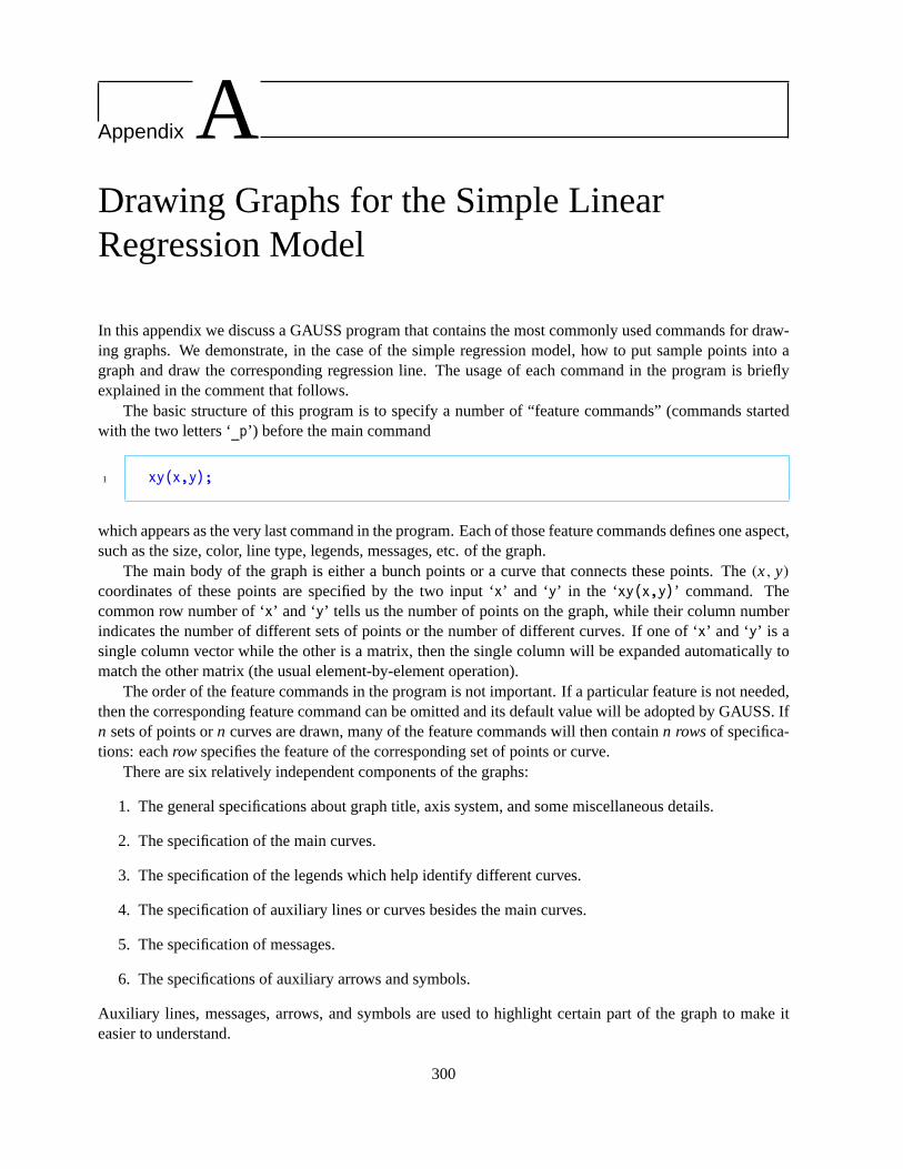
Appendix ADrawing Graphs for the Simple LinearRegression Model
In this appendix we discuss a GAUSS program that contains the most commonly used commands for draw-ing graphs. We demonstrate, in the case of the simple regression model, how to put sample points into agraph and draw the corresponding regression line. The usage of each command in the program is brieflyexplained in the comment that follows.
The basic structure of this program is to specify a number of “feature commands” (commands startedwith the two letters ‘_p’) before the main command
1 xy(x,y);
which appears as the very last command in the program. Each of those feature commands defines one aspect,such as the size, color, line type, legends, messages, etc. of the graph.
The main body of the graph is either a bunch points or a curve that connects these points. The(x, y)coordinates of these points are specified by the two input ‘x’ and ‘y’ in the ‘xy(x,y)’ command. Thecommon row number of ‘x’ and ‘y’ tells us the number of points on the graph, while their column numberindicates the number of different sets of points or the number of different curves. If one of ‘x’ and ‘y’ is asingle column vector while the other is a matrix, then the single column will be expanded automatically tomatch the other matrix (the usual element-by-element operation).
The order of the feature commands in the program is not important. If a particular feature is not needed,then the corresponding feature command can be omitted and its default value will be adopted by GAUSS. Ifn sets of points orn curves are drawn, many of the feature commands will then containn rowsof specifica-tions: eachrow specifies the feature of the corresponding set of points or curve.
There are six relatively independent components of the graphs:
1. The general specifications about graph title, axis system, and some miscellaneous details.
2. The specification of the main curves.
3. The specification of the legends which help identify different curves.
4. The specification of auxiliary lines or curves besides the main curves.
5. The specification of messages.
6. The specifications of auxiliary arrows and symbols.
Auxiliary lines, messages, arrows, and symbols are used to highlight certain part of the graph to make iteasier to understand.
300

301
The kind of graphs we create with the ‘xy(x,y)’ command in the following program is called the ‘XY’graph. GAUSS can make other graphs such as bar charts, histograms, contours, and 3-dimensional graphs.Once we are familiar with the following program for the ‘XY’ graph, exploring other types of graphs willbe fairly straightforward.
If the version of GAUSS used is 2.2 or lower, then before this graph drawing program can be executedwe need to configure GAUSS as follows: the program ‘equip’ in the subdirectory ‘\GAUSS’ has to be runonce to inform GAUSS the specifications of the computer and the printer. This program will create a filewith the name ‘config.gpc’, which is generally to be stored in the ‘\GAUSS’ subdirectory. We also need toadd the following line to the file ‘autoexec.bat’ which is in the root subdirectory.
1 set gpc=c:\gauss
The ‘autoexec.bat’ file is an ASCII file. If the version of GAUSS used is 3.0 or higher, then we only needto configure GAUSS by modifying the ASCII file ‘pqgrun.cfg’ in the ‘\GAUSS’ subdirectory to specify thecomputer and the printer we use.
Before using the following program, we must run the linear regression program for the Engel Curvemodel in chapter 5 with the following command added at the end of that program (before the ‘end’ com-mand):
1 x = x[.,2]; /* We do not need the constant term. */2
3 save x, y, b, e, seb, s2, r2;
Similarly, if the ‘ols’ command is used, then the following commands should be part of the program:
1 _olsres = 1;2
3 {vnam,mmt,b,stb,vb,seb,s2,cor,r2,e,d} = ols(0,y,x);4
5 save x, y, b, e, seb, s2, r2;
These commands save seven matrices from the estimation in the matrix file format. These matrix data willthen be loaded in the following graph program.
1 new;2 /*************************************************************************3 * Drawing Graph for the Simple Regression Model *4 *************************************************************************/5 library pgraph; /* Calling the graph program. */6 graphset; /* Resetting graphics globals to default values. */7 /* These commands are discussed in chapter 9. */8
9 load x, y, b, seb, s2, r2; /* These six matrices must have been
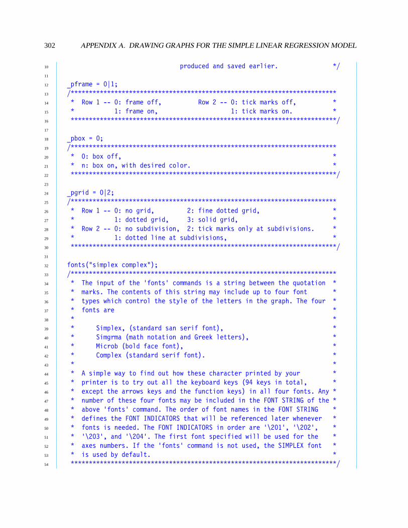
302 APPENDIX A. DRAWING GRAPHS FOR THE SIMPLE LINEAR REGRESSION MODEL
10 produced and saved earlier. */11
12 _pframe = 0|1;13 /*************************************************************************14 * Row 1 -- 0: frame off, Row 2 -- 0: tick marks off, *15 * 1: frame on, 1: tick marks on. *16 *************************************************************************/17
18 _pbox = 0;19 /*************************************************************************20 * 0: box off, *21 * n: box on, with desired color. *22 *************************************************************************/23
24 _pgrid = 0|2;25 /*************************************************************************26 * Row 1 -- 0: no grid, 2: fine dotted grid, *27 * 1: dotted grid, 3: solid grid, *28 * Row 2 -- 0: no subdivision, 2: tick marks only at subdivisions. *29 * 1: dotted line at subdivisions, *30 *************************************************************************/31
32 fonts("simplex complex");33 /*************************************************************************34 * The input of the ‘fonts’ commands is a string between the quotation *35 * marks. The contents of this string may include up to four font *36 * types which control the style of the letters in the graph. The four *37 * fonts are *38 * *39 * Simplex, (standard san serif font), *40 * Simgrma (math notation and Greek letters), *41 * Microb (bold face font), *42 * Complex (standard serif font). *43 * *44 * A simple way to find out how these character printed by your *45 * printer is to try out all the keyboard keys (94 keys in total, *46 * except the arrows keys and the function keys) in all four fonts. Any *47 * number of these four fonts may be included in the FONT STRING of the *48 * above ‘fonts’ command. The order of font names in the FONT STRING *49 * defines the FONT INDICATORS that will be referenced later whenever *50 * fonts is needed. The FONT INDICATORS in order are ‘\201’, ‘\202’, *51 * ‘\203’, and ‘\204’. The first font specified will be used for the *52 * axes numbers. If the ‘fonts’ command is not used, the SIMPLEX font *53 * is used by default. *54 *************************************************************************/
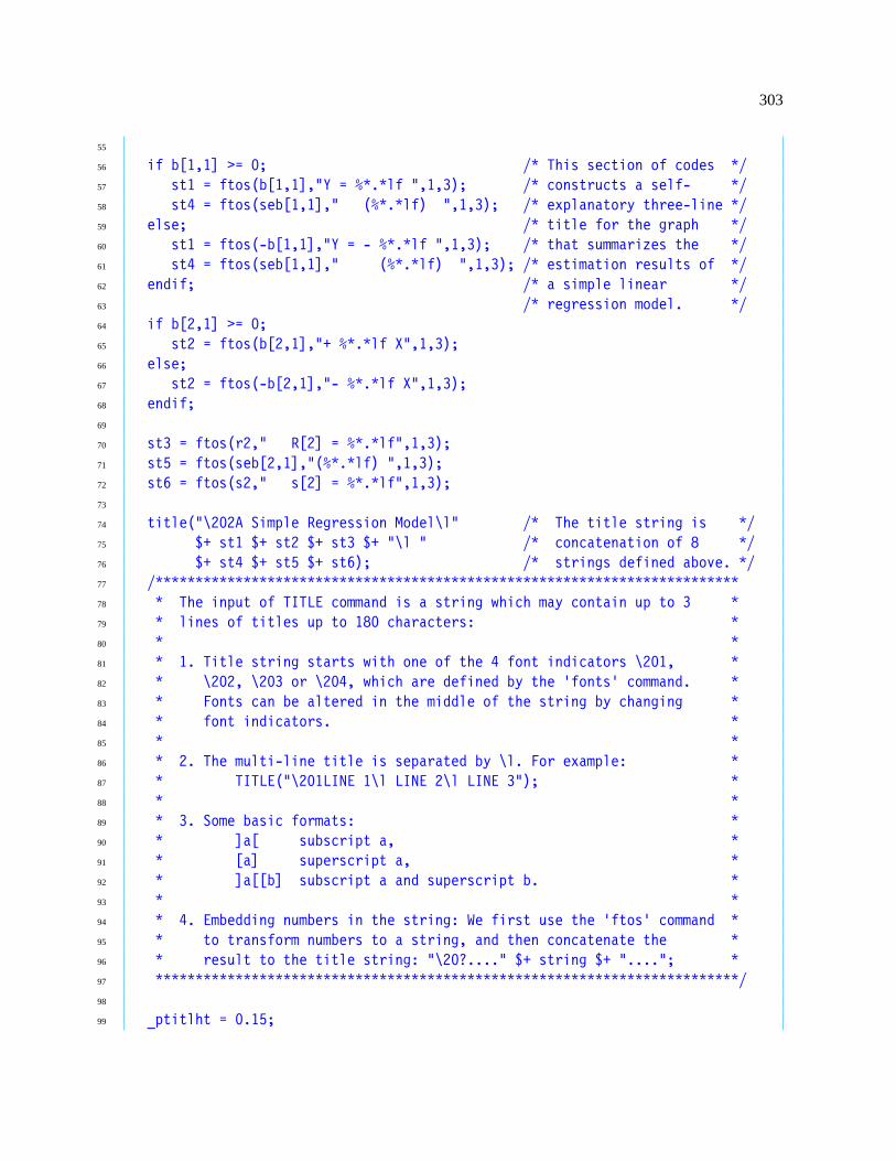
303
55
56 if b[1,1] >= 0; /* This section of codes */57 st1 = ftos(b[1,1],"Y = %*.*lf ",1,3); /* constructs a self- */58 st4 = ftos(seb[1,1]," (%*.*lf) ",1,3); /* explanatory three-line */59 else; /* title for the graph */60 st1 = ftos(-b[1,1],"Y = - %*.*lf ",1,3); /* that summarizes the */61 st4 = ftos(seb[1,1]," (%*.*lf) ",1,3); /* estimation results of */62 endif; /* a simple linear */63 /* regression model. */64 if b[2,1] >= 0;65 st2 = ftos(b[2,1],"+ %*.*lf X",1,3);66 else;67 st2 = ftos(-b[2,1],"- %*.*lf X",1,3);68 endif;69
70 st3 = ftos(r2," R[2] = %*.*lf",1,3);71 st5 = ftos(seb[2,1],"(%*.*lf) ",1,3);72 st6 = ftos(s2," s[2] = %*.*lf",1,3);73
74 title("\202A Simple Regression Model\l" /* The title string is */75 $+ st1 $+ st2 $+ st3 $+ "\l " /* concatenation of 8 */76 $+ st4 $+ st5 $+ st6); /* strings defined above. */77 /*************************************************************************78 * The input of TITLE command is a string which may contain up to 3 *79 * lines of titles up to 180 characters: *80 * *81 * 1. Title string starts with one of the 4 font indicators \201, *82 * \202, \203 or \204, which are defined by the ‘fonts’ command. *83 * Fonts can be altered in the middle of the string by changing *84 * font indicators. *85 * *86 * 2. The multi-line title is separated by \l. For example: *87 * TITLE("\201LINE 1\l LINE 2\l LINE 3"); *88 * *89 * 3. Some basic formats: *90 * ]a[ subscript a, *91 * [a] superscript a, *92 * ]a[[b] subscript a and superscript b. *93 * *94 * 4. Embedding numbers in the string: We first use the ‘ftos’ command *95 * to transform numbers to a string, and then concatenate the *96 * result to the title string: "\20?...." $+ string $+ "...."; *97 *************************************************************************/98
99 _ptitlht = 0.15;
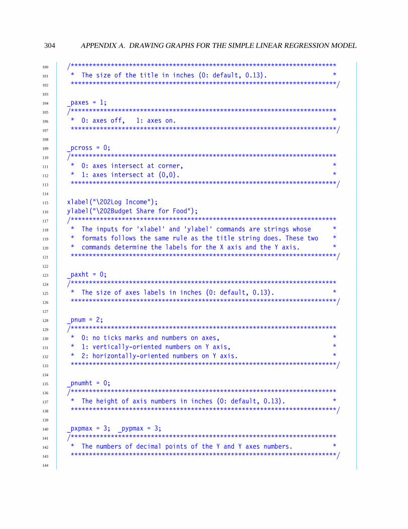
304 APPENDIX A. DRAWING GRAPHS FOR THE SIMPLE LINEAR REGRESSION MODEL
100 /*************************************************************************101 * The size of the title in inches (0: default, 0.13). *102 *************************************************************************/103
104 _paxes = 1;105 /*************************************************************************106 * 0: axes off, 1: axes on. *107 *************************************************************************/108
109 _pcross = 0;110 /*************************************************************************111 * 0: axes intersect at corner, *112 * 1: axes intersect at (0,0). *113 *************************************************************************/114
115 xlabel("\202Log Income");116 ylabel("\202Budget Share for Food");117 /*************************************************************************118 * The inputs for ‘xlabel’ and ‘ylabel’ commands are strings whose *119 * formats follows the same rule as the title string does. These two *120 * commands determine the labels for the X axis and the Y axis. *121 *************************************************************************/122
123 _paxht = 0;124 /*************************************************************************125 * The size of axes labels in inches (0: default, 0.13). *126 *************************************************************************/127
128 _pnum = 2;129 /*************************************************************************130 * 0: no ticks marks and numbers on axes, *131 * 1: vertically-oriented numbers on Y axis, *132 * 2: horizontally-oriented numbers on Y axis. *133 *************************************************************************/134
135 _pnumht = 0;136 /*************************************************************************137 * The height of axis numbers in inches (0: default, 0.13). *138 *************************************************************************/139
140 _pxpmax = 3; _pypmax = 3;141 /*************************************************************************142 * The numbers of decimal points of the Y and Y axes numbers. *143 *************************************************************************/144

305
145 /* xtics(min,max,step,div);146 ytics(min,max,step,div); */147 /*************************************************************************148 * To define scaling, axes numbering and tick marks for X and Y axes: *149 * min: the minimum value, *150 * max: the maximum value, *151 * step: the value between major tics, *152 * div: the number of subdivisions. *153 *************************************************************************/154
155 asclabel(0,0);156 /*************************************************************************157 * To set up character labels for the X and Y axes. It requires two *158 * character vectors as inputs. If any input is 0, then character *159 * labels will not be used for that axis. *160 * input 1: labels for the tick marks on the X axis, *161 * input 2: labels for the tick marks on the Y axis. *162 *************************************************************************/163
164 /************************* -- MAIN CURVES -- ****************************/165
166 _plctrl = -1;167 /*************************************************************************168 * Line control (may contain multiple rows and one row for each curve) *169 * 0: line only (default), *170 * n: ( > 0) line and symbols at every n points, *171 * n: ( < 0) symbols only at every n points, *172 * -1: symbols only at every point. *173 *************************************************************************/174
175 _pltype = 0;176 /*************************************************************************177 * Line type (one row for each line) *178 * 0: default, *179 * 1: dashed, 3: short dashed, 5: dots and dashes, *180 * 2: dotted, 4: densed dots, 6: solid. *181 *************************************************************************/182
183 _plwidth = 0;184 /*************************************************************************185 * Line thickness: 0 (normal) or greater, one row for each line *186 *************************************************************************/187
188 _psymsiz = 3;189 /*************************************************************************

306 APPENDIX A. DRAWING GRAPHS FOR THE SIMPLE LINEAR REGRESSION MODEL
190 * Symbol size: 1-9 (may have decimals) (if 0, default 5 is used) *191 *************************************************************************/192
193 _pstype = 1;194 /*************************************************************************195 * Symbol type (one row for each line) *196 * 1: circle, 6: reverse triangle, 11: solid plus, *197 * 2: square, 7: star, 12: solid diamond, *198 * 3: triangle, 8: solid circle, 13: solid reverse triangle, *199 * 4: plus, 9: solid square, 14: solid star, *200 * 5: diamond, 10: solid triangle, 0: default. *201 *************************************************************************/202
203 _pcolor = 4;204 /*************************************************************************205 * Line color (one row for each line) *206 * 0: black, 4: red, 8: grey, 12: light red, *207 * 1: blue, 5: Magenta, 9: light blue, 13: light magenta, *208 * 2: green, 6: brown, 10: light green, 14: yellow, *209 * 3: cyan, 7: white, 11: light cyan, 15: bright white. *210 *************************************************************************/211
212 _pmcolor = 15;213 /*************************************************************************214 * A row of nine numbers to define color for: *215 * row 1: axes, row 4: y axis label, row 7: box, *216 * row 2: axes numbers, row 5: z axis label, row 8: date, *217 * row 3: x axis label, row 6: title, row 9: background. *218 * If scalar, then it will be expanded to a 9x1 vector. *219 *************************************************************************/220
221 /************************** -- LEGEND -- *******************************/222
223 _plegstr = "";224 /*************************************************************************225 * Multiple legend strings are separated by \000 *226 * _plegstr = "\20?legend1\000legend2\000legend3"; *227 * See title string for other formatting possibilities. *228 *************************************************************************/229
230 _plegctl = 0;231 /*************************************************************************232 * Legend control can a scalar, or 4 element vector. *233 * 1. Scalar: 0 -- no legend (default), *234 * 1 -- a legend will be created based on _plegstr. The *

307
235 * legend box will be placed in the lower right-hand *236 * corner just inside the axes area. *237 * 2. 4 element vector: *238 * row 1: 1 -- in plot coordinates, *239 * 2 -- in inches (9.0 x 6.855), *240 * 3 -- in pixels (3120 x 4096), *241 * row 2: font size -- 1-9, can have decimals (5 default), *242 * row 3: x location of the lower left corner of legend box, *243 * row 4: y location of the lower left corner of legend box. *244 *************************************************************************/245
246 /*************************** -- MESSAGES -- ****************************/247
248 _pmsgstr = "";249 /*************************************************************************250 * Multiple massage strings are separated by \000 *251 * _msgstr = "\20?MASSAGE1\000MASSAGE2\000MASSAGE3"; *252 * See title string for other format considerations. *253 *************************************************************************/254
255 _pmsgctl = 0;256 /*************************************************************************257 * Massage control: one row for each message *258 * column 1: x location of lower left corner, *259 * column 2: y location of lower left corner, *260 * column 3: massage height in inches, *261 * column 4: rotation in degrees, *262 * column 5: 1 -- plot coordinates; 2 -- inches, *263 * column 6: color, *264 * column 7: font thickness, 0 (normal) or greater. *265 *************************************************************************/266
267 /*********************** -- AUXILIARY LINES -- *************************/268
269 _pline = 1˜6˜ /* The fitted regression */270 minc(x[.,2])˜(b[1]+minc(x[.,2])*b[2])˜ /* line is drawn on top */271 maxc(x[.,2])˜(b[1]+maxc(x[.,2])*b[2])˜ /* of the sampled points.*/272 1˜14˜0;273 /*************************************************************************274 * Line definitions: one row for each line *275 * column 1: 1 -- line in plot coordinates, *276 * 2 -- line in inches (9.0x6.855), *277 * 3 -- line in pixel(3120x4096), *278 * 4 -- circle in plot coordinates, *279 * 5 -- circle in inches (9.0x6.855), *

308 APPENDIX A. DRAWING GRAPHS FOR THE SIMPLE LINEAR REGRESSION MODEL
280 * 6 -- radius in plot coordinates, *281 * 7 -- radius in inches (9.0x6.855), *282 * column 2: line type (see above), *283 * column 3: x location of the starting point, *284 * column 4: y location of the starting point, *285 * column 5: x location of the end point, *286 * column 6: y location of the end point, *287 * column 7: 0 -- continuation; 1 -- new, *288 * column 8: color, *289 * column 9: line thickness, 0 (normal) or greater. *290 * If 0, no line will be drawn. *291 *************************************************************************/292
293 /*********************** -- AUXILIARY SYMBOLS -- ***********************/294
295 _psym = 0;296 /*************************************************************************297 * Extra symbol definitions: one row for each symbol *298 * column 1: x location of the center of the symbol, *299 * column 2: y location of the center of the symbol, *300 * column 3: symbol type, *301 * column 4: symbol size -- 1-9, can have decimals (5 default), *302 * column 5: symbol color, *303 * column 6: 1 -- inches; 2 -- plot coordinates, *304 * column 7: line thickness, 0 (normal) or greater. *305 *************************************************************************/306
307
308 /************************ -- AUXILIARY ARROWS -- ***********************/309
310 _parrow = 0;311 /*************************************************************************312 * Arrow definitions: one row for each arrow *313 * column 1: x location of the starting point, *314 * column 2: y location of the starting point, *315 * column 3: x location of the end point, *316 * column 4: y location of the end point, *317 * column 5: ratio of the arrow head length to its half width, *318 * column 6: size of arrow head in inches, *319 * column 7: fn -- type of arrow head, *320 * f is for form: *321 * 0 -- solid, *322 * 1 -- empty, *323 * 2 -- open, *324 * 3 -- closed, *

309
325 * n is for number: *326 * 0 -- none, *327 * 1 -- at the final end, *328 * 2 -- at both ends, *329 * column 8: color, *330 * column 9: 1 -- in plot coordinates, *331 * 2 -- in inches (9.0x6.855), *332 * 3 -- in pixels (3120x4096), *333 * column 10: line type (see above), *334 * column 11: line thickness, 0 (normal) or greater. *335 * If 0, no arrow will be drawn. *336 *************************************************************************/337
338
339 /************************* -- MAIN COMMAND -- ***************************/340
341 _pdate = "";342 /*************************************************************************343 * A small label on the top left corner (default: \201GAUSS). *344 * If the string is "", then nothing will be printed. *345 *************************************************************************/346
347 _ptek = "food_s.tkf";348 /*************************************************************************349 * TKF output file’s name with .TKF extension. The file can be *350 * transported and saved for later printing. no graphics file will be *351 * produced if "" is set. Default is GRAPHIC.TKF. * *352 *************************************************************************/353
354 xy(x,y);355 /*************************************************************************356 * This command directs GAUSS to draw the two dimensional graph. The *357 * two inputs are data on X and Y variables. If data on X and Y *358 * variables are multiple columns, then multiple curves will be drawn. *359 *************************************************************************/360
361 end;
After succeeding in creating a graph on the screen, we can press the ‘space bar’ to get printing selections onthe screen. These choices are self-explanatory.
Let’s consider another example where we show how to draw the scatter diagram for the residuals asopposed to the log income, which is the explanatory variable of the Engel curve model. Such a diagramis interesting because we often want to know whether there is a relationship between the residual and theexplanatory variable in a linear regression model. If there is, then some modification of the OLS estimationmay be needed. Here we only present seven commands that are required to be modified from the previous

310 APPENDIX A. DRAWING GRAPHS FOR THE SIMPLE LINEAR REGRESSION MODEL
program;
1 load x, e;2 title("\202 The Scatter Diagram for Residuals");3 _pcross = 1;4 ylabel("\202Residuals");5 _ptek = "residual.tkf";6 _pline = 0;7 xy(x[.,2],e);
Also, the ‘if...else...endif’ statements before the ‘title’ command can all be deleted.The GAUSS graph drawing capability is powerful and flexible. But with many user-friendly and even
more powerful graphic softwares available in the market, we must say that the quality of the GAUSS graphsis not particularly outstanding. Sometimes it seems to be a good idea to use GAUSS to draw a sketchy draftand then export the data to some other graphic softwares for the final version of the graph.

Appendix BGAUSS Data Set (GDS) Files
We have introduced two types of data files in chapter 2, ASCII data files and matrix files. We have alsolearned that they are mainly for smaller data sets. To store large data sets in GAUSS, we may need the thirdtype of data files – the GAUSS data set (GDS) files. In this section we explain how to use the GDS files.Here let’s first briefly list the main features of the GDS files:
1. GDS files are formulated in matrices: rows for observations and columns for variables.
2. It is possible to assign a name, the variable name, to each column and store these “variable names”along with data. The column number of a GDS file is limited only by the size of computer memory,while the row number is limited only by the size of the hard disk.
3. Each GDS is stored in a pair of files with the same file name but different extensions ‘.dat’ and ‘dht’.The file with the extension ‘.dht’ is called the header file, in which the variable names are stored.
4. Data can be stored in three levels of precision: 2 (integer precision), 4 (single precision), or 8 (doubleprecision) bytes per number. The precision level of 2 bytes per number is ideal for integers while thedouble precision is used for most real numbers. Note that matrix files are always stored in doubleprecision, which can sometimes be wasteful in terms of disk storage. For example, a 5000× 100matrix of integers requires 4,000,000 bytes, or 4 MB, of disk space if it is stored as a matrix file. Butit can be stored as a GDS file at the integer precision with only 1 MB of memory.
B.1 Writing Data to a New GAUSS Data Set
We can create a GDS file using the trio: the ‘create...with’, the ‘writer’, and the ‘close’ commands.For example, suppose we have a set of data in a 100× 5 matrix ‘xx’ left in the memory. We want to createa GDS file with the file name ‘out1” to store those 100 observations on 5 variables at the single precisionlevel, using the names ‘id’, ‘ name’, ‘ age’, ‘ var1’, and ‘region’, respectively. To do this, we first put the 5variable names in a character vector ‘varname’:
1 let varname = id name age var1 region;
and then type the following commands:
1 create fout = out1 with ˆvarname,5,4;2 check1 = writer(fout,xx);3 check2 = close(fout);
We now explain these three commands in detail:
311
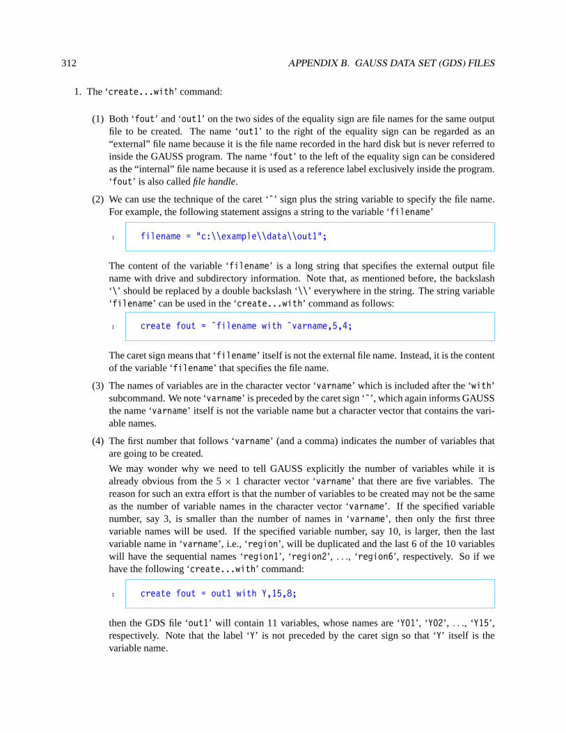
312 APPENDIX B. GAUSS DATA SET (GDS) FILES
1. The ‘create...with’ command:
(1) Both ‘fout’ and ‘out1’ on the two sides of the equality sign are file names for the same outputfile to be created. The name ‘out1’ to the right of the equality sign can be regarded as an“external” file name because it is the file name recorded in the hard disk but is never referred toinside the GAUSS program. The name ‘fout’ to the left of the equality sign can be consideredas the “internal” file name because it is used as a reference label exclusively inside the program.‘fout’ is also calledfile handle.
(2) We can use the technique of the caret ‘ˆ’ sign plus the string variable to specify the file name.For example, the following statement assigns a string to the variable ‘filename’
1 filename = "c:\\example\\data\\out1";
The content of the variable ‘filename’ is a long string that specifies the external output filename with drive and subdirectory information. Note that, as mentioned before, the backslash‘\’ should be replaced by a double backslash ‘\\’ everywhere in the string. The string variable‘filename’ can be used in the ‘create...with’ command as follows:
1 create fout = ˆfilename with ˆvarname,5,4;
The caret sign means that ‘filename’ itself is not the external file name. Instead, it is the contentof the variable ‘filename’ that specifies the file name.
(3) The names of variables are in the character vector ‘varname’ which is included after the ‘with’subcommand. We note ‘varname’ is preceded by the caret sign ‘ˆ’, which again informs GAUSSthe name ‘varname’ itself is not the variable name but a character vector that contains the vari-able names.
(4) The first number that follows ‘varname’ (and a comma) indicates the number of variables thatare going to be created.
We may wonder why we need to tell GAUSS explicitly the number of variables while it isalready obvious from the 5× 1 character vector ‘varname’ that there are five variables. Thereason for such an extra effort is that the number of variables to be created may not be the sameas the number of variable names in the character vector ‘varname’. If the specified variablenumber, say 3, is smaller than the number of names in ‘varname’, then only the first threevariable names will be used. If the specified variable number, say 10, is larger, then the lastvariable name in ‘varname’, i.e., ‘region’, will be duplicated and the last 6 of the 10 variableswill have the sequential names ‘region1’, ‘ region2’, . . ., ‘region6’, respectively. So if wehave the following ‘create...with’ command:
1 create fout = out1 with Y,15,8;
then the GDS file ‘out1’ will contain 11 variables, whose names are ‘Y01’, ‘ Y02’, . . ., ‘Y15’,respectively. Note that the label ‘Y’ is not preceded by the caret sign so that ‘Y’ itself is thevariable name.

B.1. WRITING DATA TO A NEW GAUSS DATA SET 313
(5) The last number in the ‘create...with’ command indicates the precision level, which can be 2(integer), 4 (single precision), or 8 (double precision). Double precision must be adopted if datacontain characters.
(6) Multiple ‘create...with’ commands can be used in the same program so that data may bewritten into different GDS files in the same program.
2. The ‘writer’ command:
(1) The ‘writer’ command writes the data in the matrix ‘xx’, row by row, to the GDS file, which isreferred to by the name ‘fout’ (instead ‘out1’).
(2) After the values in the ‘xx’ are completely written into ‘fout’, a scalar ‘check1’ is produced toindicate the total number of rows that have just been written.
(3) The column number of the matrix “xx’ must be the same as the variable number specified in the‘create...with’ command.
(4) Multiple ‘writer’ commands can be used after the same ‘create...with’ command. In sucha case, data will be written consecutively into the same output file.
(5) If the precision level is set at 2 and the source matrix ‘xx’ contains missing values, which areusually denoted by a dot ‘.’ in GAUSS, then these missing values will all change to the value−32768 automatically. At other levels of precision, missing values will be recorded as missingvalues.
3. The ‘close’ command closes the file ‘fout’ and creates a scalar ‘check2’ to indicate whether the fileis successfully closed: 0 for success and−1 for failure.
The ‘close’ command can be skipped since the ‘end’ command, which is usually placed at the veryend of the program, will close all the created files. The advantage of using ‘close’ command imme-diately after the file creation is that we can close the file as early as possible. If a file is not closed andthe program is terminated abnormally due to, say, power failure, then the data in the file will be lost.
A related command is
1 closeall;
which closes all files. A list of internal file names (file handles) can also follow the ‘closeall’command, in which case only the listed files will be closed. So
1 check2 = close(fout);
and
1 closeall fout;
have the same effect.
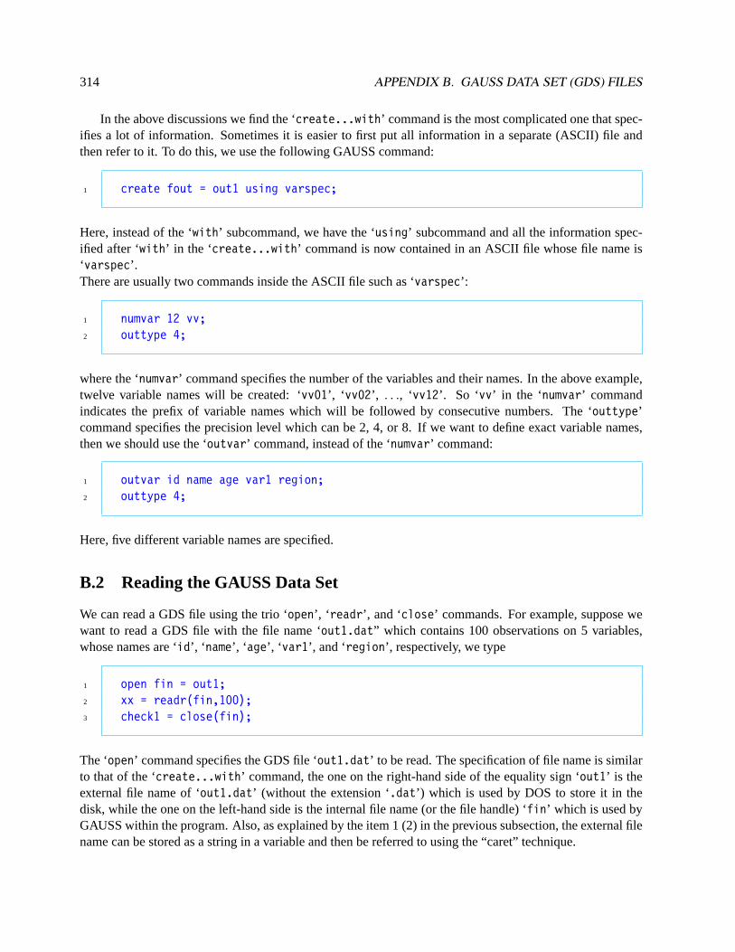
314 APPENDIX B. GAUSS DATA SET (GDS) FILES
In the above discussions we find the ‘create...with’ command is the most complicated one that spec-ifies a lot of information. Sometimes it is easier to first put all information in a separate (ASCII) file andthen refer to it. To do this, we use the following GAUSS command:
1 create fout = out1 using varspec;
Here, instead of the ‘with’ subcommand, we have the ‘using’ subcommand and all the information spec-ified after ‘with’ in the ‘create...with’ command is now contained in an ASCII file whose file name is‘varspec’.There are usually two commands inside the ASCII file such as ‘varspec’:
1 numvar 12 vv;2 outtype 4;
where the ‘numvar’ command specifies the number of the variables and their names. In the above example,twelve variable names will be created: ‘vv01’, ‘ vv02’, . . ., ‘vv12’. So ‘vv’ in the ‘numvar’ commandindicates the prefix of variable names which will be followed by consecutive numbers. The ‘outtype’command specifies the precision level which can be 2, 4, or 8. If we want to define exact variable names,then we should use the ‘outvar’ command, instead of the ‘numvar’ command:
1 outvar id name age var1 region;2 outtype 4;
Here, five different variable names are specified.
B.2 Reading the GAUSS Data Set
We can read a GDS file using the trio ‘open’, ‘ readr’, and ‘close’ commands. For example, suppose wewant to read a GDS file with the file name ‘out1.dat” which contains 100 observations on 5 variables,whose names are ‘id’, ‘ name’, ‘ age’, ‘ var1’, and ‘region’, respectively, we type
1 open fin = out1;2 xx = readr(fin,100);3 check1 = close(fin);
The ‘open’ command specifies the GDS file ‘out1.dat’ to be read. The specification of file name is similarto that of the ‘create...with’ command, the one on the right-hand side of the equality sign ‘out1’ is theexternal file name of ‘out1.dat’ (without the extension ‘.dat’) which is used by DOS to store it in thedisk, while the one on the left-hand side is the internal file name (or the file handle) ‘fin’ which is used byGAUSS within the program. Also, as explained by the item 1 (2) in the previous subsection, the external filename can be stored as a string in a variable and then be referred to using the “caret” technique.

B.3. READING AND PROCESSING DATA WITH DO-LOOPS 315
The ‘readr’ command reads rows of data from the specified file. It requires two inputs: the internalname of the file and the number of rows in the file to be read. The output is a matrix whose row numbershould of course be the same as the row number as is specified in the ‘readr’ command. The columnnumber is decided by the number of variables contained in the source GDS files. In the above example, theoutput matrix ‘xx’ will be a 100× 5 matrix. Note that even though there are 100 rows in the original GDSfiles, we do not have to read them all. We may specify 50, for example, in the above ‘readr’ command. Insuch a case only the first 50 rows will be read into the ‘xx’ matrix.
The ‘close’ command closes the opened file and indicates whether the closing is successful. See item3 in the previous subsection for more details.
B.2.1 Using Variable Names
Since the GDS file records variable names, it is possible to refer to each column of the output matrix by thecorresponding variable name. In the above example, we know the five columns of the output matrix ‘xx’are observations on the five variables ‘id’, ‘ name’, ‘ age’, ‘ var1’, and ‘region’, respectively. We can thenrefer to the five columns of ‘xx’ by ‘ iid’, ‘ iname’, ‘ iage’, ‘ ivar1’, and ‘iregion’, respectively. Here, wenote these variable names are all prefixed by ‘i’. These variable names are useful when we want to selectsome columns from ‘xx’ for some manipulation. To use this feature of the GDS file, we should add the‘varindxi’ subcommand at the end of the ‘open’ command. For example,
1 open fin = out1 varindxi;2 xx = readr(fin,100);3 check1 = close(fin);4 x1 = xx[.,iname iregion iage];5 x2 = xx[.,2 5 3];
With the ‘varindxi’ subcommand, we then have a better idea about the contents of the 100× 3 submatrix‘x1’. It contains observations on the three variables ‘name’, ‘ region’, and ‘age’ (in that order). We note thesubmatrix ‘x2’ is identical to ‘x1’. The creation of ‘x2’ is based on the equivalent but less appealing methodof indexing.
If we forget the names of the variables in a GDS file, we can use the ‘getname’ command to retrieve thevariable names. For example, to get the variable names from the GDS file ‘out1’, we use
1 name = getname("out1");2 $name;
Here, we note the external file name of the GDS is put inside the quotation marks. The output ‘name’ willbe a character vector containing the variable names. They are printed for viewing.
B.3 Reading and Processing Data with Do-Loops
Since the GDS file is mostly used to store a large number of data, trying to read all data from a large GDSfile into a matrix often causes the insufficient memory problem. We note each scalar requires 8 bytes of
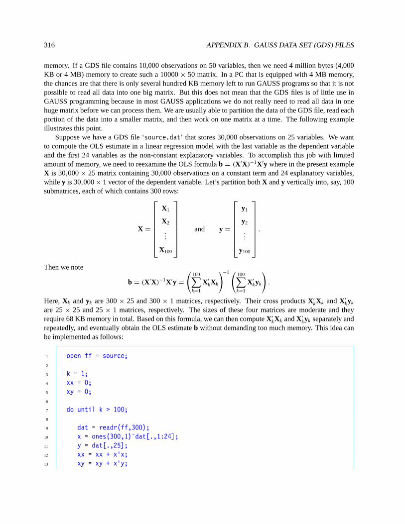
316 APPENDIX B. GAUSS DATA SET (GDS) FILES
memory. If a GDS file contains 10,000 observations on 50 variables, then we need 4 million bytes (4,000KB or 4 MB) memory to create such a 10000× 50 matrix. In a PC that is equipped with 4 MB memory,the chances are that there is only several hundred KB memory left to run GAUSS programs so that it is notpossible to read all data into one big matrix. But this does not mean that the GDS files is of little use inGAUSS programming because in most GAUSS applications we do not really need to read all data in onehuge matrix before we can process them. We are usually able to partition the data of the GDS file, read eachportion of the data into a smaller matrix, and then work on one matrix at a time. The following exampleillustrates this point.
Suppose we have a GDS file ‘source.dat’ that stores 30,000 observations on 25 variables. We wantto compute the OLS estimate in a linear regression model with the last variable as the dependent variableand the first 24 variables as the non-constant explanatory variables. To accomplish this job with limitedamount of memory, we need to reexamine the OLS formulab = (X′X)−1X′y where in the present exampleX is 30,000× 25 matrix containing 30,000 observations on a constant term and 24 explanatory variables,while y is 30,000× 1 vector of the dependent variable. Let’s partition bothX andy vertically into, say, 100submatrices, each of which contains 300 rows:
X =
X1
X2
...
X100
and y =
y1
y2
...
y100
.
Then we note
b = (X′X)−1X′y =
(100∑k=1
X′
kXk
)−1( 100∑k=1
X′
kyk
).
Here,Xk andyk are 300× 25 and 300× 1 matrices, respectively. Their cross productsX′
kXk andX′
kyk
are 25× 25 and 25× 1 matrices, respectively. The sizes of these four matrices are moderate and theyrequire 68 KB memory in total. Based on this formula, we can then computeX′
kXk andX′
kyk separately andrepeatedly, and eventually obtain the OLS estimateb without demanding too much memory. This idea canbe implemented as follows:
1 open ff = source;2
3 k = 1;4 xx = 0;5 xy = 0;6
7 do until k > 100;8
9 dat = readr(ff,300);10 x = ones(300,1)˜dat[.,1:24];11 y = dat[.,25];12 xx = xx + x’x;13 xy = xy + x’y;

B.3. READING AND PROCESSING DATA WITH DO-LOOPS 317
14 k = k + 1;15
16 endo;17 check = close(ff);18
19 b = invpd(xx)*xy;
The key idea here is the use of a do-loop.Although the logic of such a do-loop is straightforward, we may have the question: how does the ‘readr’
command works inside the do-loop? To answer this question, we have to know an important concept in usingthe ‘readr’ command.
B.3.1 The ‘readr’ and the ‘writer’ Commands and Do-Loop
After each row of the GDS file is read, GAUSS always prepares to read the next row or, we might say,GAUSS places a reading pointer at the next row for the next reading. So after the first iteration of the abovedo-loop and one hundred rows of the GDS file ‘ff’ (or ‘ source.dat’) are read into the output matrix ‘dat’,GAUSS places the reading pointer at the 101-th row of the GDS file even though that row is not immediatelyread. After the first cycle is completed and GAUSS is prepared to execute the ‘readr’ command for thesecond time, GAUSS will then follow the reading pointer and read the 101-th row of the GDS file.
In the above example the decision of partitioning the GDS file into 100 parts is somewhat arbitrary. Wenote the computation time of a do-loop is directly proportional to the number of cycles to be iterated. If thenumber of cycles is large, then the execution of the do-loop can be quite time consuming and inefficient. Soit is sometimes necessary to experiment with different partitions of the GDS file and we should always pushtoward the limit of memory by minimizing the number of partitions. For example, if we have more than 136KB of memory, then we can cut the computation time in half by reducing the partition of the GDS file ‘ff’to 50 parts, in which case eachXk will be a 200× 25 matrix.
Suppose after some further experiments we find it is possible to increase the row number of the submatrixXk to 450. But in such a case the corresponding number of partition is 67 while the last submatrix contains300 rows only which is different from that of other 66 submatrices. Nevertheless, the do-loop can still beused as usual. It should be noted that in the last iteration, the matrix ‘dat’, as well as ‘x’ and ‘y’, will contain300 rows only. Here, we will be using a special feature of the ‘readr’ command: it automatically terminateswhen the reading pointer passes over the last row of the GDS file ‘ff’.
The above program can be somewhat simplified by a new GAUSS command ‘eof’: the command linethat starts the do-loop:
1 do until k > 100;
can be replaced by
1 do until eof(ff);
The command ‘eof’ indicates whether the reading pointer passes the end of GDS file ‘ff’ or not. When itdoes, then the ‘eof(ff)’ returns the value 1 and the do-loop terminates.

318 APPENDIX B. GAUSS DATA SET (GDS) FILES
All the above discussions on how the ‘readr’ command interacts with do-loop can be extended to the‘writer’ command.
B.3.2 The ‘seekr’ Command
There is a GAUSS command “seekr’ that allows us to move the reading pointer to any row of the GDS filewe want. This command is useful when we want to read a part of the GDS file more than once or when wewant to skip some part of the GDS file. For example, given the above GDS file ‘source.dat’, we need thefirst 100 and the last 100 observations on the first variable, and the first 200 observations on the last variable,then the GAUSS program for retrieving these data is as follows:
1 open ff = source;2
3 dat = readr(ff,100);4 x1 = dat[.,1];5
6 rn1 = seekr(ff,29900);7 dat = readr(ff,100);8 x1 = x1|dat[.,1];9
10 rn2 = seekr(ff,1);11 dat = readr(ff,200);12 x3 = dat[.,25];
After the first ‘readr’ command, the reading pointer is placed at the 101-th row of the GDS file ‘ff’. But the‘seekr’ command moves the reading pointer to the 29,900-th row of the GDS file ‘ff’ so that the last 100rows can then be read directly. There is an output from the ‘seekr’ command which indicates the locationof the reading point after the ‘seekr’ command is executed. It is usually the same as the second input of the‘seekr’ command, so the value of ‘rn1’ should be 29,900. Note that the second ‘seekr’ command movesthe reading pointer back to the first row of the GDS file ‘ff’ and the value of ‘rn2’ is 1.
Note that if the ‘seekr’ command is specified as ‘rn3 = seekr(ff,0)’, then the reading pointer ismovedafter the last row of the GDS file ‘ff’ and the value of ‘rn3’ is 30,001.
B.4 GAUSS Commands That Are Related to GDS Files
Given that a GDS file is opened and is assigned an internal file name (file handle) ‘ff’, then we can use thefollowing GAUSS commands:
1 rn = rowsf(ff); /* The number of rows of the file ‘ff’. */2 cn = colsf(ff); /* The number of columns of the file ‘ff’. */3
4 pl = typef(ff); /* The value of ‘pl’ is either 2, 4, or 8, which is5 the precision level of the data in the file ‘ff’.*/

B.4. GAUSS COMMANDS THAT ARE RELATED TO GDS FILES 319
If we want to get the variable names from a GDS file without first opening it, we can use
1 vname = getname("source");
The input of this command is a string containing the name of GDS file and the output is a character vectorof the variable names.
B.4.1 Sorting the GDS File
In subsection 8.3 we mentioned the GAUSS command ‘sortc’ that sorts a matrix (rearrange the order ofthe rows) according the values of one of its column. If we want to sort a GDS file directly, then use
1 sortd("source","sortout","VAR11",-1);
Here, the first input indicates the GDS file that is to be sorted. The sorted file will be another GDS file whosename is given by the second input. The third input specifies the column number or the variable name whosevalues will be used as the “key” for ordering. Note that the first three inputs are all included in quotationmarks so that they are all strings. If the third input is the column number, then it can be a scalar (a numbernot inside quotation marks). The last input can take four possible values: 1 and−1 mean the values of thekey variable are numeric, while 1 (-1) causes the rows to be the sorted in ascending (descending) order;2 and−2 mean the key is a character variable, while 2 (-2) causes the rows to be the sorted in ascending(descending) order. Note that the ‘sortd’ command does not have matrix output.
B.4.2 The ‘ols’ Command and the GDS File
When we first discussed the ‘ols’ command in subsection 16.8, we mentioned it took three inputs whilethere we set the first input to 0 without explanation. Now with the knowledge of GDS files, we are ready formore discussions on the ‘ols’ command. We can directly use the data in a GDS file for the OLS estimation.Suppose the GDS file we want to use is ‘source.dat’ again. Let’s assume the 25 variables in this data sethave the variable names ‘VAR01’, ‘ VAR02’, . . ., ‘VAR25’, respectively. If we want to run an OLS estimationwith ‘VAR07’ as the dependent variable and ‘VAR12’, ‘ VAR06’, ‘ VAR21’, ‘ VAR17’, and ‘VAR01’ as regressors,then the GAUSS commands are
1 rgssor = {"VAR12","VAR06","VAR21","VAR17","VAR01"};2 {vnam,mmt,b,stb,vb,seb,s2,cor,r2,e,d} = ols("source","VAR07",rgssor);
or, equivalently,
1 rgssor = {12, 6, 21, 17, 1};2 {vnam,mmt,b,stb,vb,seb,s2,cor,r2,e,d} = ols("source",7,rgssor);
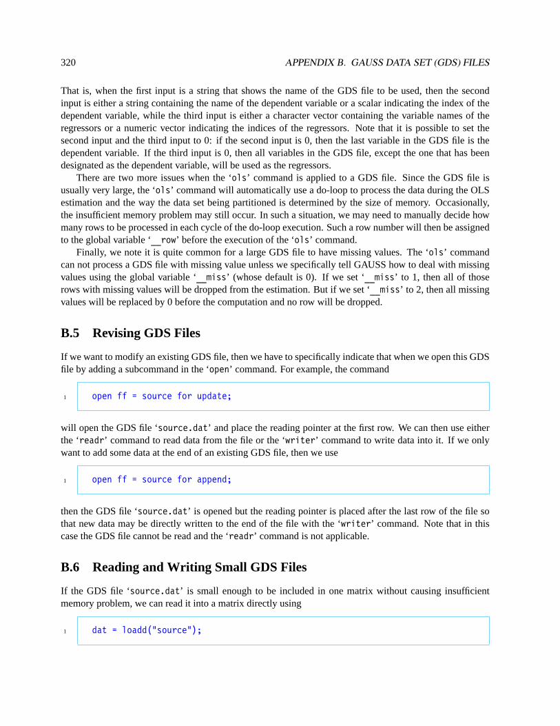
320 APPENDIX B. GAUSS DATA SET (GDS) FILES
That is, when the first input is a string that shows the name of the GDS file to be used, then the secondinput is either a string containing the name of the dependent variable or a scalar indicating the index of thedependent variable, while the third input is either a character vector containing the variable names of theregressors or a numeric vector indicating the indices of the regressors. Note that it is possible to set thesecond input and the third input to 0: if the second input is 0, then the last variable in the GDS file is thedependent variable. If the third input is 0, then all variables in the GDS file, except the one that has beendesignated as the dependent variable, will be used as the regressors.
There are two more issues when the ‘ols’ command is applied to a GDS file. Since the GDS file isusually very large, the ‘ols’ command will automatically use a do-loop to process the data during the OLSestimation and the way the data set being partitioned is determined by the size of memory. Occasionally,the insufficient memory problem may still occur. In such a situation, we may need to manually decide howmany rows to be processed in each cycle of the do-loop execution. Such a row number will then be assignedto the global variable ‘__row’ before the execution of the ‘ols’ command.
Finally, we note it is quite common for a large GDS file to have missing values. The ‘ols’ commandcan not process a GDS file with missing value unless we specifically tell GAUSS how to deal with missingvalues using the global variable ‘__miss’ (whose default is 0). If we set ‘__miss’ to 1, then all of thoserows with missing values will be dropped from the estimation. But if we set ‘__miss’ to 2, then all missingvalues will be replaced by 0 before the computation and no row will be dropped.
B.5 Revising GDS Files
If we want to modify an existing GDS file, then we have to specifically indicate that when we open this GDSfile by adding a subcommand in the ‘open’ command. For example, the command
1 open ff = source for update;
will open the GDS file ‘source.dat’ and place the reading pointer at the first row. We can then use eitherthe ‘readr’ command to read data from the file or the ‘writer’ command to write data into it. If we onlywant to add some data at the end of an existing GDS file, then we use
1 open ff = source for append;
then the GDS file ‘source.dat’ is opened but the reading pointer is placed after the last row of the file sothat new data may be directly written to the end of the file with the ‘writer’ command. Note that in thiscase the GDS file cannot be read and the ‘readr’ command is not applicable.
B.6 Reading and Writing Small GDS Files
If the GDS file ‘source.dat’ is small enough to be included in one matrix without causing insufficientmemory problem, we can read it into a matrix directly using
1 dat = loadd("source");
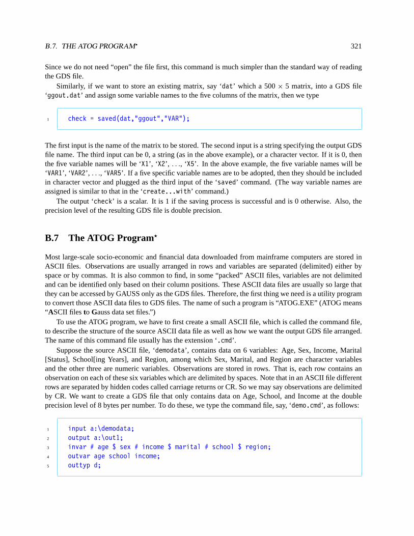
B.7. THE ATOG PROGRAM? 321
Since we do not need “open” the file first, this command is much simpler than the standard way of readingthe GDS file.
Similarly, if we want to store an existing matrix, say ‘dat’ which a 500× 5 matrix, into a GDS file‘ggout.dat’ and assign some variable names to the five columns of the matrix, then we type
1 check = saved(dat,"ggout","VAR");
The first input is the name of the matrix to be stored. The second input is a string specifying the output GDSfile name. The third input can be 0, a string (as in the above example), or a character vector. If it is 0, thenthe five variable names will be ‘X1’, ‘ X2’, . . ., ‘X5’. In the above example, the five variable names will be‘VAR1’, ‘ VAR2’, . . ., ‘VAR5’. If a five specific variable names are to be adopted, then they should be includedin character vector and plugged as the third input of the ‘saved’ command. (The way variable names areassigned is similar to that in the ‘create...with’ command.)
The output ‘check’ is a scalar. It is 1 if the saving process is successful and is 0 otherwise. Also, theprecision level of the resulting GDS file is double precision.
B.7 The ATOG Program?
Most large-scale socio-economic and financial data downloaded from mainframe computers are stored inASCII files. Observations are usually arranged in rows and variables are separated (delimited) either byspace or by commas. It is also common to find, in some “packed” ASCII files, variables are not delimitedand can be identified only based on their column positions. These ASCII data files are usually so large thatthey can be accessed by GAUSS only as the GDS files. Therefore, the first thing we need is a utility programto convert those ASCII data files to GDS files. The name of such a program is “ATOG.EXE” (ATOG means“ASCII filesto Gauss data set files.”)
To use the ATOG program, we have to first create a small ASCII file, which is called the command file,to describe the structure of the source ASCII data file as well as how we want the output GDS file arranged.The name of this command file usually has the extension ‘.cmd’.
Suppose the source ASCII file, ‘demodata’, contains data on 6 variables: Age, Sex, Income, Marital[Status], School[ing Years], and Region, among which Sex, Marital, and Region are character variablesand the other three are numeric variables. Observations are stored in rows. That is, each row contains anobservation on each of these six variables which are delimited by spaces. Note that in an ASCII file differentrows are separated by hidden codes called carriage returns or CR. So we may say observations are delimitedby CR. We want to create a GDS file that only contains data on Age, School, and Income at the doubleprecision level of 8 bytes per number. To do these, we type the command file, say, ‘demo.cmd’, as follows:
1 input a:\demodata;2 output a:\out1;3 invar # age $ sex # income $ marital # school $ region;4 outvar age school income;5 outtyp d;

322 APPENDIX B. GAUSS DATA SET (GDS) FILES
The ‘input’ command specifies the name and the location of the source ASCII file, which in the presentexample contains 6 columns of data. The ‘output’ command specifies the name of the output GDS files,which causes two files ‘out1.dat’ and ‘out1.dht’ to be created.
The ‘invar’ command specifies the names and the types (character or numeric) of the variables in thesource ASCII file. Note that the variable names are not part of the source ASCII file but arbitrarily assignedby us here in the command file. Variable names are preceded by either ‘$’ or ‘ #’ depending on whether thevariable is character or numeric. The indicators ‘$’ and ‘#’ can be omitted, in which case the type of variableis the same as the previous one. If none of the indicator is specified at all, then all variables are considerednumeric.
The ‘outvar’ command specifies the variables to be included in the output GDS files and the outputvariables can be in any designated order. The ‘outtyp’ command specifies the precision level of the outputGDS. Three options are available: ‘d’ for double precision, ‘f’ for single precision (which is the default),and ‘i’ for integer precision.
If in the ‘invar’ and ‘outvar’ commands the variable names are in sequence, such as the seven variables‘rec01’, ‘ rec02’, ..., ‘rec07’, then these sequential variable names can be abbreviated as ‘rec[7]’. Also,three sequential variable names like ‘xx4’, ‘ xx5’, and ‘xx6’ can be abbreviated as ‘xx[4:6]’.
To execute the ATOG program in the GAUSS command mode, we type
1 atog demo;
Note that the file extension ‘.cmd’ is not needed in the above command. But if the name of the commandfile has an extension different from ‘.cmd’, then the extension needs to be fully specified.
B.7.1 The Structure of the Source ASCII file
Because the data in the source ASCII file may be arranged in a variety of formats, we will have to provide allthe necessary information to the ATOG program through the ‘invar’ command. More specifically, variablesin the source ASCII file can be delimited in three different ways so that the corresponding ‘invar’ commandhas three basic formats:
1. If the variables in the source ASCII file are delimited by spaces, commas, or CR, then we only need asimple ‘invar’ command that specifies variable names together with their types (# for numeric valuesand & for characters). The above example illustrates such a case.
(1) Strictly speaking, observations do not have to be listed in rows and delimited by CR. For exam-ple, in the above example each row may contain 18, instead of 6, values. With 6 variable namesbeing specified in the ‘invar’ command, the ATOG program will treat the 18 values in each rowas three sets of observations. That is, different observations do not have to be delimited by CRso that they appear in different rows. Spaces that separate values are treated just the same as theCR that separate rows and vice versa.
(2) Multiple spaces or commas with no data in between will be ignored and considered as a singlespace or comma.
(3) Missing values should be recorded as a period ‘.’.

B.7. THE ATOG PROGRAM? 323
2. If the variables in the source ASCII file are delimited by some characters (which are called the delim-iter and can be any printable characters including commas), then we add the ‘delimit’ subcommandimmediately after the ‘invar’ command to inform the ATOG program what character is used as thedelimiter. When the ‘delimit’ subcommand is used, then any pair of delimiters with no values inbetween imply a missing value which is equivalent to a period ‘.’ between the pair of delimiters.
The ‘delimit’ subcommand allows two inputs. Let’s consider the following examples.
(1) If the delimiter is ‘;’ and we expect one delimiter after every variable, then we type
1 invar delimit(;n) zz[5];
Here, the first input ‘;’ of the ‘delimit’ subcommand specifies the delimiter. The second input‘n’ of the ‘delimit’ subcommand indicates one delimiter after every variable. So there is adelimiter even after the last variable in each row. In the above example where five variables arespecified in the ‘invar’ command, five ‘;’ are expected in each row. If a row contains less thanfive ‘;’, then that row is considered incomplete and willnotbe included in the output GDS file.
(2) If the delimiter is ‘*’ and we do not expect a delimiter after the last variables, then we type
1 invar delimit(*) zz[5];
Here, the first input ‘*’ of the ‘delimit’ subcommand specifies the delimiter. There is nosecond input for the ‘delimit’ subcommand, which implies that there is a delimiter betweentwo variables but no delimiter is expected after the last variable. So with five variables specifiedin the ‘invar’ command, only four delimiters are expected in each row.
(3) If the delimiter is ‘,’ and we do not expect a delimiter after the last variables, then we type
1 invar delimit zz[5];
Here, there is no input for the ‘delimit’ subcommand since the character ‘,’ happens to be thedefault delimiter. Also, with five variables specified in the ‘invar’ command, only four commasare expected in each row.
(4) If each row only contains one value onlywhile blank rows are considered missing, then we givethe ‘delimit’ subcommand the special input ‘\n’:
1 invar delimit(\n) zz[5];
(5) There is another special input ‘\r’ for the ‘delimit’ subcommand:
1 invar delimit(\r) zz[5];
which specifies the following: there are five values in each row, the delimiter is comma ‘,’, andno comma after the last variable is expected.
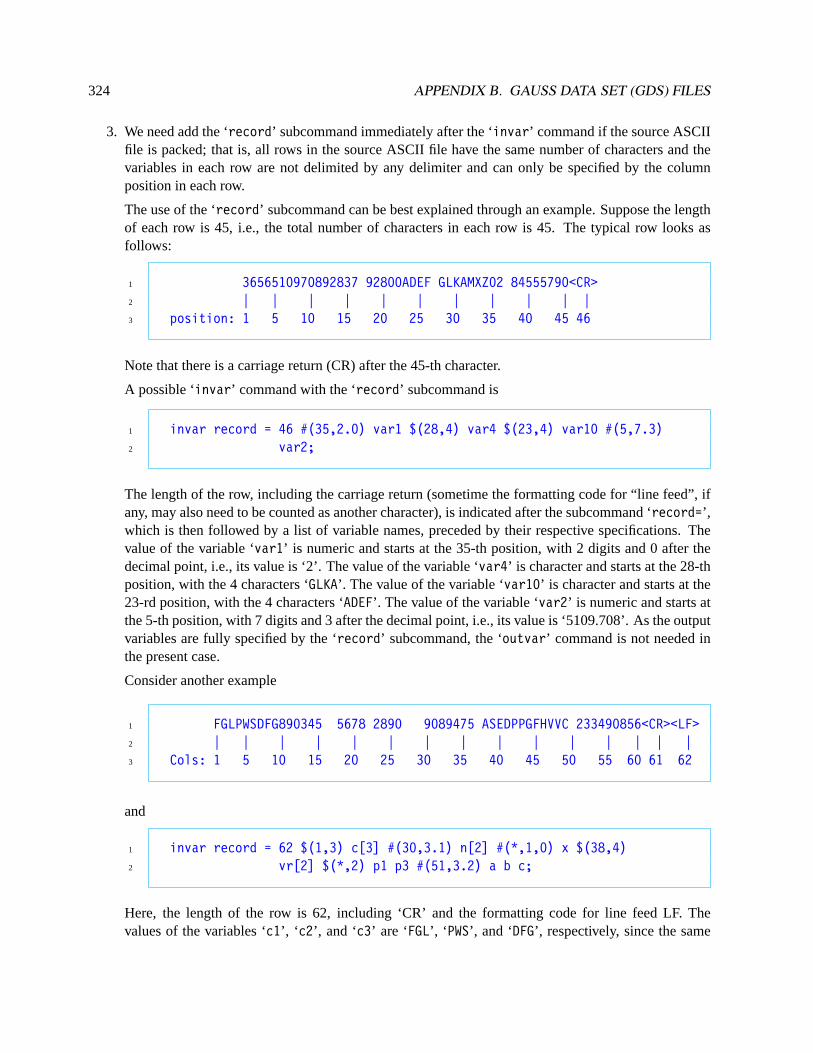
324 APPENDIX B. GAUSS DATA SET (GDS) FILES
3. We need add the ‘record’ subcommand immediately after the ‘invar’ command if the source ASCIIfile is packed; that is, all rows in the source ASCII file have the same number of characters and thevariables in each row are not delimited by any delimiter and can only be specified by the columnposition in each row.
The use of the ‘record’ subcommand can be best explained through an example. Suppose the lengthof each row is 45, i.e., the total number of characters in each row is 45. The typical row looks asfollows:
1 3656510970892837 92800ADEF GLKAMXZ02 84555790<CR>2 | | | | | | | | | | |3 position: 1 5 10 15 20 25 30 35 40 45 46
Note that there is a carriage return (CR) after the 45-th character.
A possible ‘invar’ command with the ‘record’ subcommand is
1 invar record = 46 #(35,2.0) var1 $(28,4) var4 $(23,4) var10 #(5,7.3)2 var2;
The length of the row, including the carriage return (sometime the formatting code for “line feed”, ifany, may also need to be counted as another character), is indicated after the subcommand ‘record=’,which is then followed by a list of variable names, preceded by their respective specifications. Thevalue of the variable ‘var1’ is numeric and starts at the 35-th position, with 2 digits and 0 after thedecimal point, i.e., its value is ‘2’. The value of the variable ‘var4’ is character and starts at the 28-thposition, with the 4 characters ‘GLKA’. The value of the variable ‘var10’ is character and starts at the23-rd position, with the 4 characters ‘ADEF’. The value of the variable ‘var2’ is numeric and starts atthe 5-th position, with 7 digits and 3 after the decimal point, i.e., its value is ‘5109.708’. As the outputvariables are fully specified by the ‘record’ subcommand, the ‘outvar’ command is not needed inthe present case.
Consider another example
1 FGLPWSDFG890345 5678 2890 9089475 ASEDPPGFHVVC 233490856<CR><LF>2 | | | | | | | | | | | | | | |3 Cols: 1 5 10 15 20 25 30 35 40 45 50 55 60 61 62
and
1 invar record = 62 $(1,3) c[3] #(30,3.1) n[2] #(*,1,0) x $(38,4)2 vr[2] $(*,2) p1 p3 #(51,3.2) a b c;
Here, the length of the row is 62, including ‘CR’ and the formatting code for line feed LF. Thevalues of the variables ‘c1’, ‘ c2’, and ‘c3’ are ‘FGL’, ‘ PWS’, and ‘DFG’, respectively, since the same
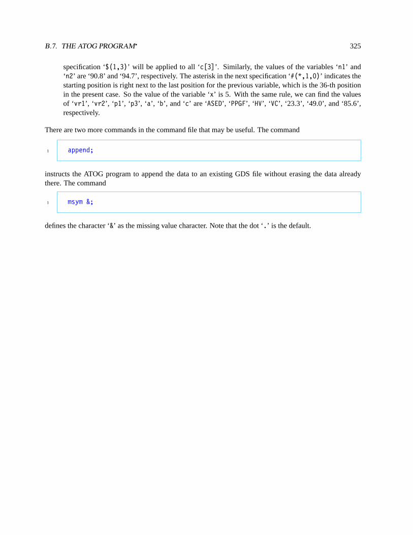
B.7. THE ATOG PROGRAM? 325
specification ‘$(1,3)’ will be applied to all ‘c[3]’. Similarly, the values of the variables ‘n1’ and‘n2’ are ‘90.8’ and ‘94.7’, respectively. The asterisk in the next specification ‘#(*,1,0)’ indicates thestarting position is right next to the last position for the previous variable, which is the 36-th positionin the present case. So the value of the variable ‘x’ is 5. With the same rule, we can find the valuesof ‘vr1’, ‘ vr2’, ‘ p1’, ‘ p3’, ‘ a’, ‘ b’, and ‘c’ are ‘ASED’, ‘ PPGF’, ‘ HV’, ‘ VC’, ‘23.3’, ‘49.0’, and ‘85.6’,respectively.
There are two more commands in the command file that may be useful. The command
1 append;
instructs the ATOG program to append the data to an existing GDS file without erasing the data alreadythere. The command
1 msym &;
defines the character ‘&’ as the missing value character. Note that the dot ‘.’ is the default.