Embed Size (px)
Citation preview
2.4 Gauss and Gauss-Jordan Methods
Ayman Hashem Sakka
Islamic University of GazaFaculty of Science
Department of Mathematics
First Semester 2013-2014
Ayman Hashem Sakka 2.4 Gauss and Gauss-Jordan Methods
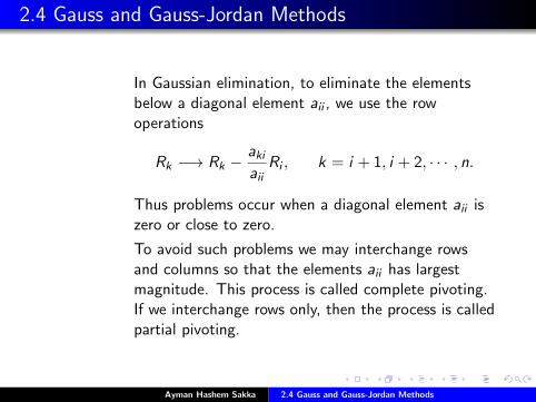
2.4 Gauss and Gauss-Jordan Methods
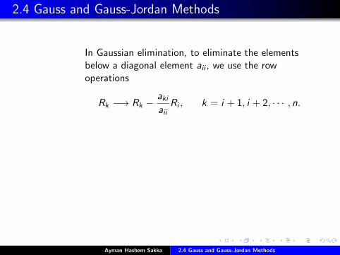
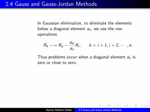
In Gaussian elimination, to eliminate the elementsbelow a diagonal element aii , we use the rowoperations
Rk −→ Rk −akiaii
Ri , k = i + 1, i + 2, · · · , n.
Thus problems occur when a diagonal element aii iszero or close to zero.
To avoid such problems we may interchange rowsand columns so that the elements aii has largestmagnitude. This process is called complete pivoting.If we interchange rows only, then the process is calledpartial pivoting.
Ayman Hashem Sakka 2.4 Gauss and Gauss-Jordan Methods
2.4 Gauss and Gauss-Jordan Methods
In Gaussian elimination, to eliminate the elementsbelow a diagonal element aii , we use the rowoperations
Rk −→ Rk −akiaii
Ri , k = i + 1, i + 2, · · · , n.
Thus problems occur when a diagonal element aii iszero or close to zero.
To avoid such problems we may interchange rowsand columns so that the elements aii has largestmagnitude. This process is called complete pivoting.If we interchange rows only, then the process is calledpartial pivoting.
Ayman Hashem Sakka 2.4 Gauss and Gauss-Jordan Methods
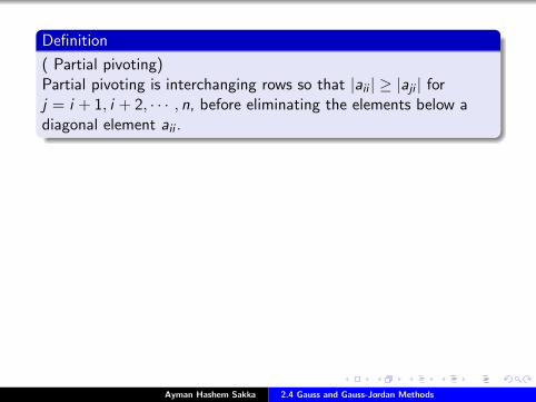
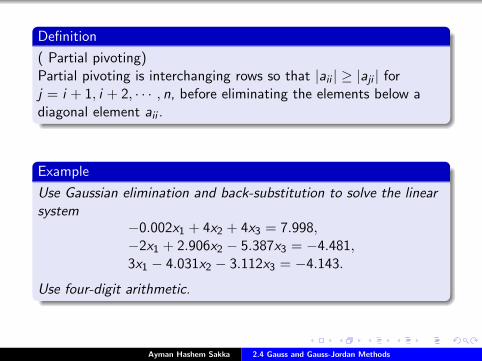
Definition
( Partial pivoting)Partial pivoting is interchanging rows so that |aii | ≥ |aji | forj = i + 1, i + 2, · · · , n, before eliminating the elements below adiagonal element aii .
Example
Use Gaussian elimination and back-substitution to solve the linearsystem
−0.002x1 + 4x2 + 4x3 = 7.998,−2x1 + 2.906x2 − 5.387x3 = −4.481,3x1 − 4.031x2 − 3.112x3 = −4.143.
Use four-digit arithmetic.
Ayman Hashem Sakka 2.4 Gauss and Gauss-Jordan Methods
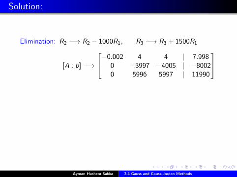
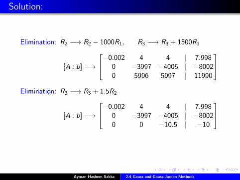
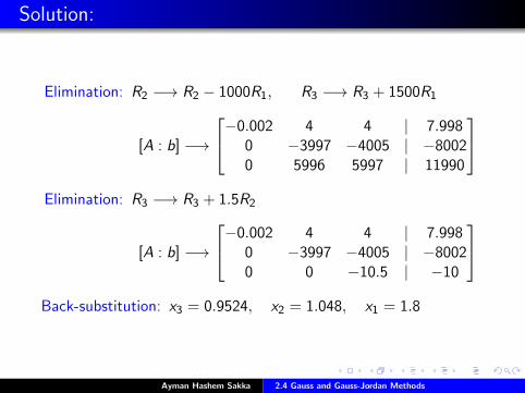
Solution:
Elimination: R2 −→ R2 − 1000R1, R3 −→ R3 + 1500R1
[A : b] −→
−0.002 4 4 | 7.9980 −3997 −4005 | −80020 5996 5997 | 11990
Elimination: R3 −→ R3 + 1.5R2
[A : b] −→
−0.002 4 4 | 7.9980 −3997 −4005 | −80020 0 −10.5 | −10
Back-substitution: x3 = 0.9524, x2 = 1.048, x1 = 1.8
Ayman Hashem Sakka 2.4 Gauss and Gauss-Jordan Methods
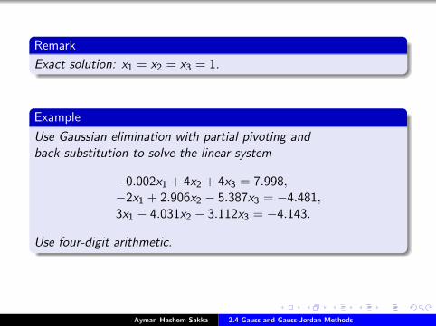
Remark
Exact solution: x1 = x2 = x3 = 1.
Example
Use Gaussian elimination with partial pivoting andback-substitution to solve the linear system
−0.002x1 + 4x2 + 4x3 = 7.998,−2x1 + 2.906x2 − 5.387x3 = −4.481,3x1 − 4.031x2 − 3.112x3 = −4.143.
Use four-digit arithmetic.
Ayman Hashem Sakka 2.4 Gauss and Gauss-Jordan Methods
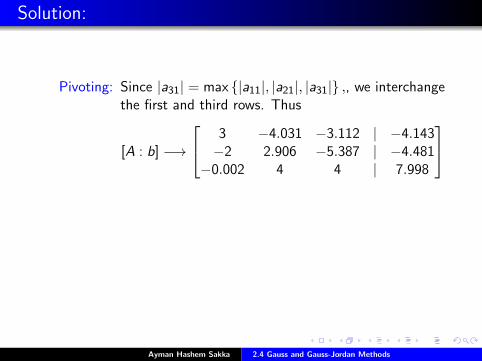
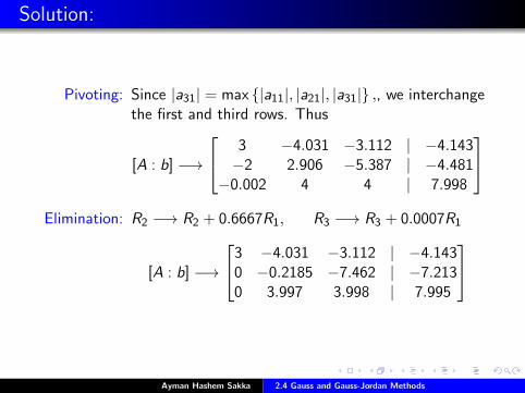
Solution:
Pivoting: Since |a31| = max {|a11|, |a21|, |a31|} ,, we interchangethe first and third rows. Thus
[A : b] −→
3 −4.031 −3.112 | −4.143−2 2.906 −5.387 | −4.481−0.002 4 4 | 7.998
Elimination: R2 −→ R2 + 0.6667R1, R3 −→ R3 + 0.0007R1
[A : b] −→
3 −4.031 −3.112 | −4.1430 −0.2185 −7.462 | −7.2130 3.997 3.998 | 7.995
Ayman Hashem Sakka 2.4 Gauss and Gauss-Jordan Methods
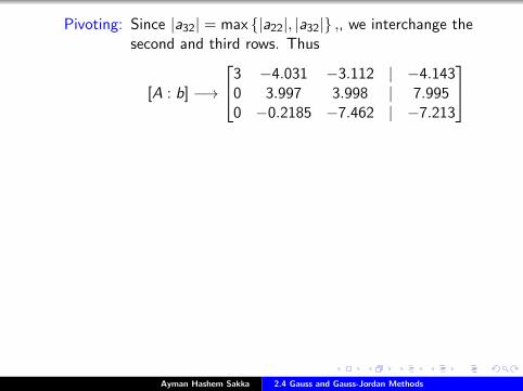
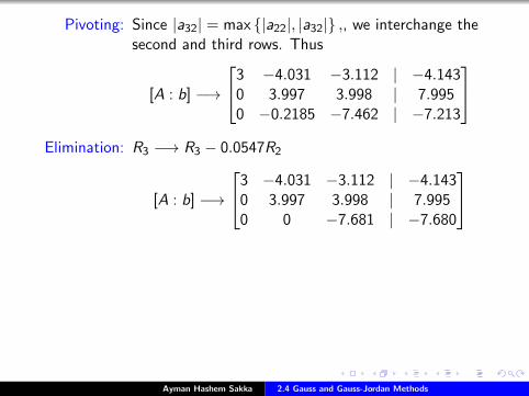
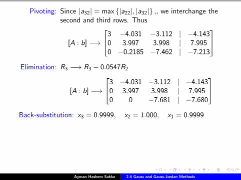
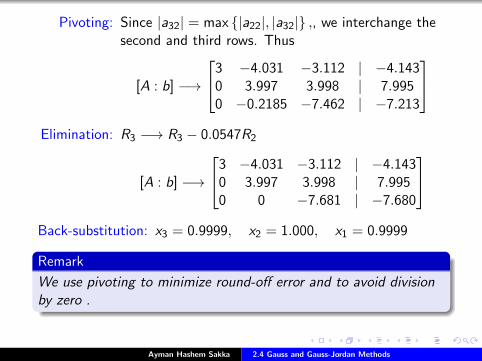
Pivoting: Since |a32| = max {|a22|, |a32|} ,, we interchange thesecond and third rows. Thus
[A : b] −→
3 −4.031 −3.112 | −4.1430 3.997 3.998 | 7.9950 −0.2185 −7.462 | −7.213
Elimination: R3 −→ R3 − 0.0547R2
[A : b] −→
3 −4.031 −3.112 | −4.1430 3.997 3.998 | 7.9950 0 −7.681 | −7.680
Back-substitution: x3 = 0.9999, x2 = 1.000, x1 = 0.9999
Remark
We use pivoting to minimize round-off error and to avoid divisionby zero .
Ayman Hashem Sakka 2.4 Gauss and Gauss-Jordan Methods
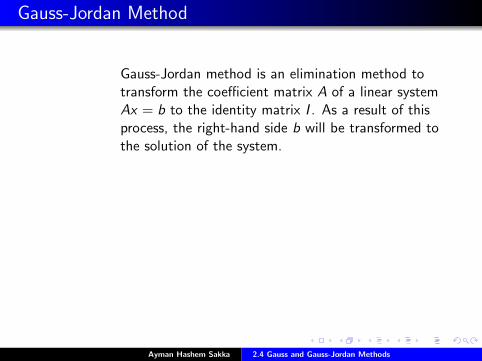
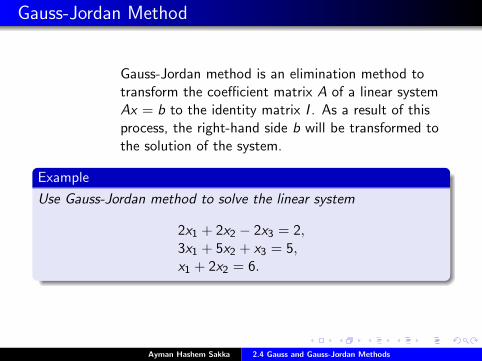
Gauss-Jordan Method
Gauss-Jordan method is an elimination method totransform the coefficient matrix A of a linear systemAx = b to the identity matrix I . As a result of thisprocess, the right-hand side b will be transformed tothe solution of the system.
Example
Use Gauss-Jordan method to solve the linear system
2x1 + 2x2 − 2x3 = 2,3x1 + 5x2 + x3 = 5,x1 + 2x2 = 6.
Ayman Hashem Sakka 2.4 Gauss and Gauss-Jordan Methods
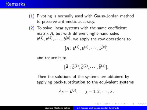
Remarks
(1) Pivoting is normally used with Gauss-Jordan methodto preserve arithmetic accuracy.
(2) To solve linear systems with the same coefficientmatrix A, but with different right-hand sidesb(1), b(2), · · · , b(k), we apply the row operations to
[A : b(1), b(2), · · · , b(k)]
and reduce it to
[A : b(1), b(2), · · · , b(k)].
Then the solutions of the systems are obtained byapplying back-substitution to the equivalent systems
Ax = b(j), j = 1, 2, · · · , k .
Ayman Hashem Sakka 2.4 Gauss and Gauss-Jordan Methods
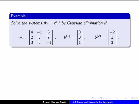
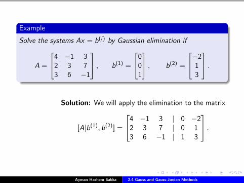
Example
Solve the systems Ax = b(i) by Gaussian elimination if
A =
4 −1 32 3 73 6 −1
, b(1) =
001
, b(2) =
−213
.
Solution: We will apply the elimination to the matrix
[A|b(1), b(2)] =
4 −1 3 | 0 −22 3 7 | 0 13 6 −1 | 1 3
.
Ayman Hashem Sakka 2.4 Gauss and Gauss-Jordan Methods
Example
Solve the systems Ax = b(i) by Gaussian elimination if
A =
4 −1 32 3 73 6 −1
, b(1) =
001
, b(2) =
−213
.
Solution: We will apply the elimination to the matrix
[A|b(1), b(2)] =
4 −1 3 | 0 −22 3 7 | 0 13 6 −1 | 1 3
.
Ayman Hashem Sakka 2.4 Gauss and Gauss-Jordan Methods
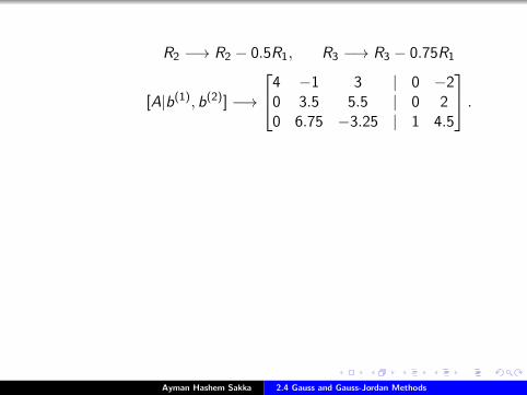
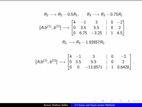
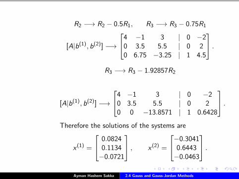
R2 −→ R2 − 0.5R1, R3 −→ R3 − 0.75R1
[A|b(1), b(2)] −→
4 −1 3 | 0 −20 3.5 5.5 | 0 20 6.75 −3.25 | 1 4.5
.
R3 −→ R3 − 1.92857R2
[A|b(1), b(2)] −→
4 −1 3 | 0 −20 3.5 5.5 | 0 20 0 −13.8571 | 1 0.6428
.Therefore the solutions of the systems are
x (1) =
0.08240.1134−0.0721
, x (2) =
−0.30410.6443−0.0463
.
Ayman Hashem Sakka 2.4 Gauss and Gauss-Jordan Methods
R2 −→ R2 − 0.5R1, R3 −→ R3 − 0.75R1
[A|b(1), b(2)] −→
4 −1 3 | 0 −20 3.5 5.5 | 0 20 6.75 −3.25 | 1 4.5
.R3 −→ R3 − 1.92857R2
[A|b(1), b(2)] −→
4 −1 3 | 0 −20 3.5 5.5 | 0 20 0 −13.8571 | 1 0.6428
.
Therefore the solutions of the systems are
x (1) =
0.08240.1134−0.0721
, x (2) =
−0.30410.6443−0.0463
.
Ayman Hashem Sakka 2.4 Gauss and Gauss-Jordan Methods
R2 −→ R2 − 0.5R1, R3 −→ R3 − 0.75R1
[A|b(1), b(2)] −→
4 −1 3 | 0 −20 3.5 5.5 | 0 20 6.75 −3.25 | 1 4.5
.R3 −→ R3 − 1.92857R2
[A|b(1), b(2)] −→
4 −1 3 | 0 −20 3.5 5.5 | 0 20 0 −13.8571 | 1 0.6428
.Therefore the solutions of the systems are
x (1) =
0.08240.1134−0.0721
, x (2) =
−0.30410.6443−0.0463
.Ayman Hashem Sakka 2.4 Gauss and Gauss-Jordan Methods
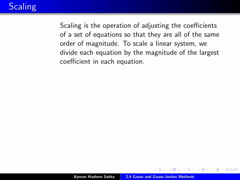
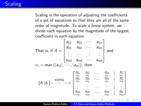
Scaling
Scaling is the operation of adjusting the coefficientsof a set of equations so that they are all of the sameorder of magnitude. To scale a linear system, wedivide each equation by the magnitude of the largestcoefficient in each equation.
That is, if A =
a11 a12 · · · a1na21 a22 · · · a2n
... · · ·...
...am1 am2 · · · amn
and
αi = max {|ai1|, · · · , |ain|}, then
[A |b ]−scaling− −→
a11α1
a12α1
· · · a1nα1
| b1α1
a21α2
a22α2
· · · a2nα2
| b2α2
...... · · ·
... |...
am1αm
am2αm
· · · amnαm
| bmαm
Ayman Hashem Sakka 2.4 Gauss and Gauss-Jordan Methods
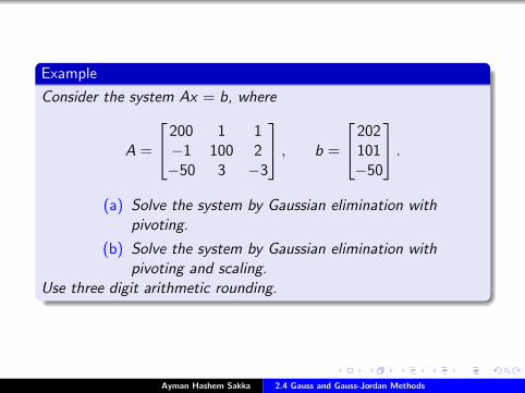
Example
Consider the system Ax = b, where
A =
200 1 1−1 100 2−50 3 −3
, b =
202101−50
.(a) Solve the system by Gaussian elimination with
pivoting.
(b) Solve the system by Gaussian elimination withpivoting and scaling.
Use three digit arithmetic rounding.
Ayman Hashem Sakka 2.4 Gauss and Gauss-Jordan Methods
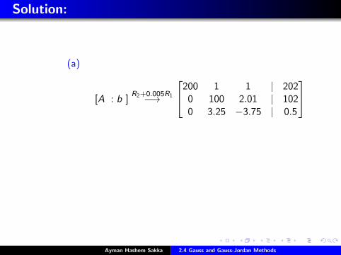
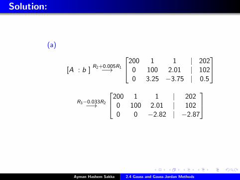
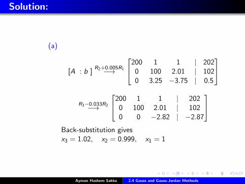
Solution:
(a)
[A : b ]R2+0.005R1−→
200 1 1 | 2020 100 2.01 | 1020 3.25 −3.75 | 0.5
R3−0.033R2−→
200 1 1 | 2020 100 2.01 | 1020 0 −2.82 | −2.87
Back-substitution givesx3 = 1.02, x2 = 0.999, x1 = 1
Ayman Hashem Sakka 2.4 Gauss and Gauss-Jordan Methods
Solution:
(a)
[A : b ]R2+0.005R1−→
200 1 1 | 2020 100 2.01 | 1020 3.25 −3.75 | 0.5
R3−0.033R2−→
200 1 1 | 2020 100 2.01 | 1020 0 −2.82 | −2.87
Back-substitution givesx3 = 1.02, x2 = 0.999, x1 = 1
Ayman Hashem Sakka 2.4 Gauss and Gauss-Jordan Methods
Solution:
(a)
[A : b ]R2+0.005R1−→
200 1 1 | 2020 100 2.01 | 1020 3.25 −3.75 | 0.5
R3−0.033R2−→
200 1 1 | 2020 100 2.01 | 1020 0 −2.82 | −2.87
Back-substitution givesx3 = 1.02, x2 = 0.999, x1 = 1
Ayman Hashem Sakka 2.4 Gauss and Gauss-Jordan Methods
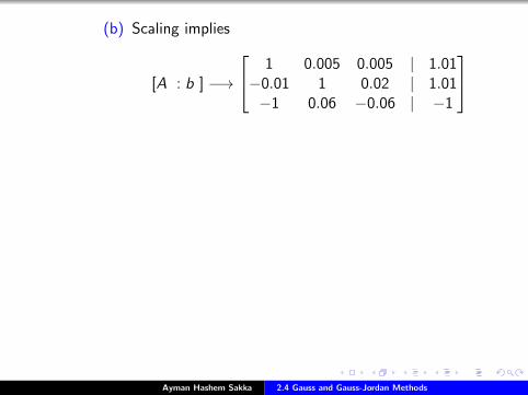
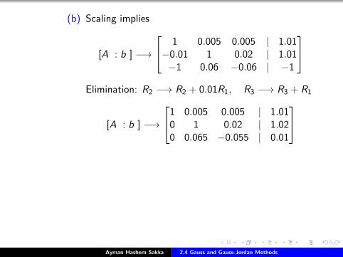
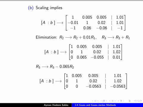
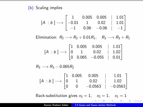
(b) Scaling implies
[A : b ] −→
1 0.005 0.005 | 1.01−0.01 1 0.02 | 1.01−1 0.06 −0.06 | −1
Elimination: R2 −→ R2 + 0.01R1, R3 −→ R3 + R1
[A : b ] −→
1 0.005 0.005 | 1.010 1 0.02 | 1.020 0.065 −0.055 | 0.01
R3 −→ R3 − 0.065R2
[A : b ] −→
1 0.005 0.005 | 1.010 1 0.02 | 1.020 0 −0.0563 | −0.0563
Back-substitution gives x3 = 1, x2 = 1, x1 = 1
Ayman Hashem Sakka 2.4 Gauss and Gauss-Jordan Methods
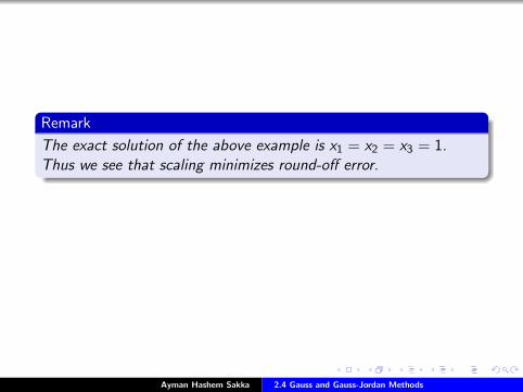
Remark
The exact solution of the above example is x1 = x2 = x3 = 1.Thus we see that scaling minimizes round-off error.
Ayman Hashem Sakka 2.4 Gauss and Gauss-Jordan Methods

Remark
The exact solution of the above example is x1 = x2 = x3 = 1.Thus we see that scaling minimizes round-off error.
Ayman Hashem Sakka 2.4 Gauss and Gauss-Jordan Methods


![Gauss jordan[1]](https://img.dokumen.tips/doc/110x75/55a4a35b1a28abb6308b4621/gauss-jordan1.jpg)