Learning Directed Acyclic Graphs with Mixed Effects

1

Learning Directed Acyclic Graphs with MixedEffects Structural Equation Models fromObservational DataXiang Li 1,†, Shanghong Xie 2,†, Peter McColgan 3, Sarah J. Tabrizi 3,4, Rachael I. Scahill 3,Donglin Zeng 5 and Yuanjia Wang 2,6,⇤

1Statistics and Decision Sciences, Janssen Research & Development, LLC, Raritan,NJ, U.S.A.2Department of Biostatistics, Mailman School of Public Health, Columbia University,New York, NY, U.S.A.3Huntington’s Disease Centre, Department of Neurodegenerative Disease, UCLInstitute of Neurology, London, WC1N 3BG, UK.4National Hospital for Neurology and Neurosurgery, Queen Square, London, UnitedKingdom5Department of Biostatistics, University of North Carolina, Chapel Hill, NorthCarolina, U.S.A.6Departments of Psychiatry, Columbia University Medical Center, New York, NY,U.S.A.†These authors have contributed equally to this work and are joint first authors.Correspondence*:Corresponding [email protected]

ABSTRACT2

The identification of causal relationships between random variables from large-scale3observational data using directed acyclic graphs (DAG) is highly challenging. We propose4a new mixed-effects structural equation model (mSEM) framework to estimate subject-specific5DAGs, where we represent joint distribution of random variables in the DAG as a set of structural6causal equations with mixed effects. The directed edges between nodes depend on observed7exogenous covariates on each of the individual and unobserved latent variables. The strength8of the connection is decomposed into a fixed-effect term representing the average causal9effect given the covariates and a random effect term representing the latent causal effect10due to unobserved pathways. The advantage of such decomposition is to capture essential11asymmetric structural information and heterogeneity between DAGs in order to allow for the12identification of causal structure with observational data. In addition, by pooling information13across subject-specific DAGs, we can identify causal structure with a high probability and14estimate subject-specific networks with a high precision. We propose a penalized likelihood-15based approach to handle multi-dimensionality of the DAG model and a fast computational16algorithm to achieve desirable sparsity by hard-thresholding the edges. We theoretically prove17the identifiability of mSEM. Using simulations and an application to protein signaling data, we18show substantially improved performances when compared to existing methods and consistent19

1

Li et al.

results with a network estimated from interventional data. Lastly, we identify gray matter atrophy20networks in regions of brain from patients with Huntington’s disease and corroborate our findings21using white matter connectivity data collected from an independent study.22

Keywords: Graphical models, Network analysis, Causal structure discovery, Heterogeneity, Regularization23

1 INTRODUCTION

Directed acyclic graphs (DAGs) are used to represent the causal mechanisms of a complex system ofinteracting components, such as biological cellular pathways [1], gene regulatory networks [2], and brainconnectivity networks [3]. The ability to identify causal relations between variables in observational data ishighly challenging. Specifically, given a set of centered random variables M = (M1, · · · ,Mp)

0, referred toas nodes, the causal relationship between these nodes in a DAG can be represented by a structural equationmodel (SEM) [4]:

Mj = fj(pa(j), "j), j = 1, · · · , p,

where pa(j) is the set of parental nodes of Mj , and "j is a random variable representing unexplained24variation. In many applications, M is assumed to follow a multivariate Gaussian distribution satisfying a25linear SEM,26

Mj =X

k2pa(j)

✓jkMk + "j , "j ⇠ N(0, �

2j ); j = 1, · · · , p, (1)

where B = (✓jk) is referred to as an adjacency matrix.27

Estimation of DAG structure (i.e., parental sets pa(j)) is non-deterministic polynomial-time hard (NP-28hard) because the number of possible DAGs grows super-exponentially with the number of nodes [5].29Mainly two types of methods are proposed to tackle this challenge, namely, independence-based [e.g., 6]30and score-based [e.g., 7] methods. The independence-based approaches calculate the partial correlation31between any pair of nodes and perform statistical tests to assess the conditional dependence. A popular32method is the PC algorithm [6], which has been proven to be uniformly consistent for estimating ultra33high-dimensional, sparse DAGs [8]. The PC algorithm was modified as PC-stable to remove its dependence34on node ordering [9]. A limitation of the PC algorithm is that it does not provide the proper level of multiple35comparison correction and thus may lead to a large number of false positives in practice. To remedy this36limitation, a hybrid, two-stage approach was proposed [PenPC, 10] that first estimates a sparse skeleton37based on penalized regression and then performs a modified PC-stable algorithm on the skeleton.38

The score-based approach searches for the DAG using a pre-specified score criterion, such as Bayesian39Information Criterion (BIC) or penalized likelihood function. As it is not computationally feasible to search40through the space of all DAGs, a two-phase greedy equivalence search algorithm explores an equivalence41class based on BIC by adding and deleting edges. With additional information on node ordering, the42estimation of DAG is equivalent to neighbourhood selection for which several penalized likelihood43approaches have been developed [11, 12]. More recently, attempts have been made to estimate a DAG44without knowing the node ordering [13, 14]. Other recent developments include leveraging asymmetric45information between nodes [15, 16] or exploring the invariance property of causal relation using combined46observational and interventional data [17]. Simulation studies suggest that independence-based methods47perform adequately for identifying the skeleton of a DAG from observational data [18]. However, these48

This is a provisional file, not the final typeset article 2

Li et al.

methods may perform worse for identifying the causal direction than some search-and-score methods that49exploit the asymmetric distributional information [18].50

All of the existing DAG estimation methods assume homogeneity of the causal effect of the underlying51DAG model in (1) (i.e., ✓jk is common across individuals in the population). However, there is a growing52body of evidence suggesting that biological networks may depend on subject-specific characteristics53such as genomic markers [19, 20, 21]. For mental disorders, individual differences in edge strength in54comorbidity networks have been widely observed [22]. Modeling heterogeneity of network effects may55improve interpretability, biological relevance, and predictability. This area is much less explored with the56exception of a few methods proposed to study subject-specific undirected graphical models. For example, a57conditional Gaussian graphical model with covariate-adjusted mean but homogeneous precision matrix has58been considered [23, 24].To characterize heterogeneous dependence structure between groups, [25] jointly59estimated graphical models that share common structure but also allowed for differences between networks.60Recently, instead of modeling groups separately, [26] directly incorporated covariates into an Ising model61in order to build a covariate-dependent undirected graph. A common assumption of these approaches is62that the dependence between two nodes is fully explained by the observed exogenous covariates. Such63an assumption may not be satisfied in many biological and clinical applications due to the presence of64unexplained latent residual heterogeneity representing hidden pathways between nodes. [27] proposed a65Bayesian approach to estimate DAG by including non-Gaussian latent variables in a linear SEM, but does66not estimate individual-specific graphs.67

Our goal in this article is to develop a novel method and an efficient estimation procedure to study68covariate-dependent DAGs with latent effect modification in multi-dimensional settings. Our method69is based on mixed-effects SEM (mSEM) and penalized likelihood to obtain DAG structure and causal70effects simultaneously. The covariates are treated as exogenous variables, and their joint distribution is71not of interest. The key difference between mSEM and current approaches is that the causal effect, ✓jk72in Model (1), is random and varies across individuals. To capture variation of the manifestation of causal73relationship among individuals, our model allows the magnitude of the edge strength to be heterogeneous74across subjects, while keeping the direction of causal relationship to be homogeneous. The heterogeneous75causal magnitude is modeled by both fixed effects that depend on observed covariates and random effects76that capture unexplained heterogeneity.77

We propose a two-stage approach to estimate mSEM, whereby the first stage performs neighborhood78selection by maximizing a penalized likelihood to identify a sparse skeleton, and the second stage searches79for the DAG by solving an approximate `0-penalty problem via hard-thresholding within the identified80skeleton, followed by an easily implemented DAG-checking procedure. We show theoretical proof of81the identifiability (the graph is unique) of our model. Through extensive simulations and application to a82well-known protein signaling study [1], we show substantially improved performance in terms of robustness83and accuracy when compared to existing methods, including PC and penPC, and consistent performance84when compared to analysis using interventional data. Lastly, we apply the proposed method to discover the85causal dependence relationship among regions of brain atrophy from patients with Huntington’s disease86(HD) [28] and corroborate our findings in an independent study [29].87

2 METHODOLOGY

For the ith subject, let M i = (Mi1,Mi2, · · · ,Mip)0 denote p random variables or nodes in a DAG. Let88

Xi = (1, Xi1, Xi2, · · · , Xiq)0 denote a q + 1-dimensional vector including a constant and q exogenous89

Frontiers 3

Li et al.

covariates that may modify the causal network among components in M i. We consider a mixed-effects90model in which the causal effect depends on both fixed effects of observed variables Xi and unobserved91random effects {�ijk}. For the jth node, the mSEM is given by:92

Mij =X

k2pa(j)(�T

jkXi + �ijk)Mik + "ij , (2)

where �jk is the vector of fixed effects (including an intercept and effects associated with Xi), and93�ijk is the unexplained heterogeneity of causal effects beyond Xi. We assume that �ijk are independent94and follow N(0, �

2jk) and the independent error terms "ij follow N(0, �

2"j ). The SEM in (2) assumes that95

for each edge in the DAG, the causal effect is decomposed into a subject-specific fixed-effect term that96depends on the exogenous covariates (i.e., �T

jkXi) and a subject-specific random-effect term that captures97residual heterogeneity in causal effects due to other latent factors beyond Xi (i.e., �ijk). When �jk = 098and �

2jk 6= 0, the causal dependence between j and k is explained by unobserved latent factors but not Xi.99

No causal effect between node j and k corresponds to �jk = 0 and �

2jk = 0.100

In this work, we assume that the ordering of causal dependence or the parental sets are unknown, and101propose methods to simultaneously learn the ordering and structure of DAG and the parameters in the SEM.102Previous literature has pointed out that qualitative capacity claims about causal effects are invariant across103different populations of subjects, whereas the quantitative claims in SEM often are population-specific104[e.g., 30, Chapter 7]. Thus, we assume that the qualitative causal dependence (set of nodes and directed105edges) is homogeneous among subjects while the magnitude of the edge strength varies across subjects.106Presence of an edge from Mik to Mij is defined as �jk 6= 0 or �2jk 6= 0; otherwise, there is no causal effect107

from Mik to Mij . Note that when the components of �jk associated with covariates Xil are zero and �

2jk108

are zero, the subject-specific DAG model in (2) reduces to a homogeneous DAG model in (1). We express109the model for M i given �ijk in matrix form as110

M i =�

B(Xi) + �i�

M i + "i (3)

where B(Xi) is a matrix of fixed effects with entry (j, k) as �TjkXi and the diagonal elements as111

zeros, �i is a matrix of random effects with entry (j, k) as �ijk and the diagonal elements as zeros, and112"i = ("i1, "i2, · · · , "ip)0 is a vector of error terms. Note that the joint distribution of M in Model (3) is113non-Gaussian due to random effects in �i, where the asymmetric information on the distribution between114nodes can facilitate inference on the causal network from the observational data.115

To estimate a DAG, we use a likelihood-based approach. Given the random effects �i, the conditional116likelihood function of M i is given by117

p(M i;Xi|�i) / |E|�1/2|I �B(Xi)� �i|⇥

exp

✓

�1

2

MTi (I �B(Xi)� �i)

TE�1(I �B(Xi)� �i)M i

◆

,

(4)

where Cov["i] = E is a diagonal matrix of �2"j .118

To simplify presentation, we introduce the notation for the vectorized �i and define non-zero components119of vectorized �i as �i = {�ijk : �

2jk > 0}. Then, �i can be expressed as a linear combination of120

components in �i as �i =P

�2jk>0 �ijkHjk, where Hjk is a single-entry matrix with one entry (j, k).121


Li et al.

Denote by Cov[�i] = G the covariance matrix of �i. The observed likelihood function is given by122

nY

i=1

Z

�i

p(M i;Xi|�i)p(�i)d�i, (5)

where p(�i) / |G|�1/2exp

�

��Ti G

�1�i/2�

.123

Under the DAG assumption of no directed cycle, B(Xi) + �i can always be transformed into an upper124diagonal matrix after some unknown permutation of the rows and columns. Therefore, the determinant125|I �B(Xi)� �i| in the likelihood function (4) is one. The integral in the likelihood (5) can be explicitly126calculated and the negative log-likelihood function is given by127

ln =

nX

i=1

pX

j=1

0

B

@

⇣

Mij �P

k 6=j

�

�TjkXi

�

Mik

⌘2

P

k 6=j �2jkM

2ik + �

2"j

+ log

0

@

X

k 6=j

�

2jkM

2ik + �

2"j

1

A

1

C

A

(6)

up to a constant. Thus, parameter estimation in the likelihood is separable, leading to a great computational128advantage. With a small number of nodes, in order to minimize the negative log-likelihood function (6), one129can alternatively solve the weighted least squares to update {�jk : j = 1, · · · , p; k = 1, · · · , p} and use130the Newton-Raphson algorithm to update {�2jk : j = 1, · · · , p; k = 1, · · · , p} and {�2"j : j = 1, · · · , p}131until convergence. The identifiability of parameters in the model is shown in Theorem 1 in Section 2.3.132

2.1 Initial Sparse Graph133

With a large number of nodes, minimizing (6) would result in a full graph with all non-null estimates134of�

�jk

and �

2jk. Without any constraint on the estimates, the graph may potentially involve many false135

positive edges. To accommodate the large number of nodes, we propose to use a penalized likelihood136to choose an initial sparse graph skeleton and search for the optimum of (6) within this reduced graph137space. Based on model (2), the marginal expectation and variance of Mij are

P

k 6=j

�

�TjkXi

�

Mik and138

�

2"j +

P

k 6=j �2jkM

2ik, respectively. Define Rij = Mij �

P

k 6=j

�

�TjkXi

�

Mik. By the method of moments,139

we obtain initial estimates of the graph by minimizing the following objective functionsPn

i=1

⇣

Mij �140P

k 6=j

�

�TjkXi

�

Mik

⌘2and

Pni=1

⇣

R

2ij � �

2"j �

P

k 6=j �2jkM

2ik

⌘2for each j with j = 1, · · · , p. In order to141

obtain an initial sparse graph, `1-norm penalty can be included to minimize the objective function and142obtain initial estimates

�

e�jk

,�

e�

2jk

, and�

e�

2"j

:143

pX

j=1

0

@

nX

i=1

⇣

Mij �X

k 6=j

�

�TjkXi

�

Mik

⌘2+ �1

X

k 6=j

k�jkk1

1

A

,

pX

j=1

0

@

nX

i=1

⇣

e

R

2ij � �

2"j �

X

k 6=j

�

2jkM

2ik

⌘2+ �2

X

k 6=j

�

2jk

1

A

,

subject to �

2"j > 0, �

2jk � 0,

(7)

Frontiers 5

Li et al.

where e

Rij is Rij with �jk replaced by e�jk, the parameter estimated from minimizing the first objective144function of � at the current iteration. Here we use the same tuning parameter across nodes j = 1, · · · , p145for illustration, although in practice node-specific tuning parameter can be used at the price of increasing146computational burden. In cases where the topology of the graph varies greatly across nodes, different147tuning parameters can be used. Given a regularization path with varying �1 and �2, we select the optimal148�

⇤1 and �

⇤2 using the BIC criteria and apply the corresponding estimates as the initial skeleton. We set the149

edge (j, k) of the initial graph as null if e�jk = 0 and e�2jk = 0.150

2.2 Algorithms for Estimating DAG with Mixed-Effects Model (DAG-MM) and151Justification152

The initial graph, although asymptotically consistent[31], may not satisfy the DAG constraint due to153that estimated b�jk 6= 0 and b�kj 6= 0 or b�jk 6= 0 and b�kj 6= 0. Define graph A (set of nodes, edges, and154

edge strength) as the set of non-null edgesn

(j, k) :

q

k�jkk22/q + �

2jk > 0

o

in the skeleton resulting from155

(7). Let ✓A =

�

�jk, �2jk : (j, k) 2 A; �

2"j : j = 1, · · · , p

be the parameters for graph A and nA be the156number of non-zero edges of A. To obtain a sparse DAG, a direct approach is to constrain the number of157edges in the graph by optimizing a regularized likelihood:158

min ln(✓A), subject to A is a DAG and nA < C, (8)

where C is a tuning parameter controlling the number of edges in A. The constraints in (8) guarantee the159estimated graph is a DAG and also perform edge selection. However, the optimization in (8) is NP-hard,160because one needs to evaluate all possible graphs that satisfy the constraint nA < C. Furthermore, the161computational challenge is elevated due to the acyclic constraint.162

Instead, we perform hard-thresholding to approximately solve the `0-norm constrained optimization163problem in (8). Specifically, after the estimates in b✓A are obtained for a given graph skeleton A, we perform164

hard-threshold on the estimated edge weights by removing the edge with the smallestq

kb�jkk22/q + b�

2jk165

from A and then update the graph A. Given an updated graph A, we then start from the estimates obtained166in the previous iteration and update the estimate b✓A. This procedure continues until some criterion of167optimality is met. In our implementation, we use BIC as the criterion to select the optimal graph.168

The above procedure can be summarized into a DAG-MM algorithm (described in Algorithm 1). The tasks169include identifying graph structure (set of nodes and edges), direction of edges, and edge strength. DAG-170MM consists of three main steps: estimation of sparse skeleton and edge strength, edge orientation, and171iterative DAG building. In the first step, each node’s Markov blanket is identified by penalized likelihood172and edge strength is obtained. In the second step, edge orientation is performed by removing directionalities173with weak dependence (computed from fixed-effects parameters and variances of random effects). In the174third step, an iterative procedure performs edge pruning using the norm of the edge connection strength175and searches for the DAG that satisfies the acyclic constraint using a general and fast routine described in a176DAG-Checking algorithm (described in Algorithm 2 in Supplementary Material Section S1).177

Algorithm 1 is computationally efficient for several reasons: the sparse skeleton reduces the search space178of DAGs; ranking by the magnitude of edge effects provides search paths in the DAG space; selection179criteria BIC is only calculated when the log-likelihood (6) is the correct model (i.e., the acyclic constraint180is satisfied); and the optimal graph is selected from candidate DAGs. We observe empirically that the full181


Li et al.

Algorithm 1: DAG with mixed model (DAG-MM)1.Sparse skeleton: Estimate an initial sparse graph AI by solving the objective

function (7). Obtain the estimates b✓AIby minimizing (6) for AI .

2.Edge orientation: Initialize AR = AI . For (j, k) belongs to {(j, k) : (j, k) 2 AR and (k, j) 2 AR},prune the initial graph:

a.Calculate cjk =

q

kb�jkk22/q + b�

2jk and rjk = cjk/ckj for all

(j, k) 2 {(j, k) : (j, k) 2 AR and (k, j) 2 AR}.b.Remove the edge (j, k), where (j, k) = argminj,k rjk;

update AR = AR \ (j, k).c.Update the estimate b✓AR

by minimizing (6) for AR.3.Iterative DAG building: Initialize A1 = AR. For i = 1, · · · , p ⇤ (p� 1)/2 or untilAi = ;, search DAG with hard-thresholding:

a.Update the estimate b✓Ai by minimizing (6) for Ai.b.Calculate BIC if Ai is a DAG.c.Perform edge pruning by removing the edge (j, k) with the smallest

q

kb�jkk22/q + b�

2jk. Obtain the

updated graph Ai+1 = Ai \ (j, k), and checkwhether Ai+1 satisfies acyclic constraint by Algorithm 2 if Ai is not a DAG.

graph shrinks to a DAG very fast in only a few iterations of the third step. For implementation, we have182developed main routines in C++ codes with an R interface (R program available upon request).183

2.3 Rationale of DAG-MM Algorithm and Theoretical Result184

Essentially DAG-MM uses the likelihood function as the objective function in the optimization and thus185belongs to the class of score-based approaches for estimating DAG. Similar to other score-based methods186in this class [7], the search is performed locally at each iteration. The first step provides a sparse skeleton187and consistent initial estimators of DAG edge strength through moment estimation, with the magnitude188of estimated effects close to the truth parameter values. In the second step, the direction that maximizes189the network edge strength is selected. The rationale is that the overall edge strength under the correct190direction is greater than the strength under the incorrect one (which is close to null effect). In the third step,191the DAG with the lowest BIC objective function is selected. Under the identifiability result in Theorem1921 shown below, the optima is uniquely identified, and the DAG-MM algorithm may converge in a local193neighborhood of true parameters.194

Next, we prove the identifiability of the DAG-MM procedure. Here we omit the subscript i corresponding195to subjects. For any matrix B = {�jk}j,k and ⌃ = {�2jk}j,k, we call (B,⌃) to be compatible with DAG,196denoted by (B,⌃) ⇠ DAG, if the edge pair (j, k) such that �jk 6= 0 or �jk 6= 0 forms a DAG network.197Furthermore, we use L(B,⌃, ✓) to denote the likelihood function associated with (B,⌃) using the SEM,198where ✓ = (�

2"1 , ..., �

2"p)

T . Note that if (B,⌃) ⇠ DAG, then |I � B(X)� �| = 1, so199

L(B,⌃, ✓) = exp

8

<

:

�pX

j=1

2

4

(Mj �P

k 6=j(�TjkX)Mk)

2

P

k 6=j �2jkM

2k + �

2"j

+ log(

X

k 6=j

�

2jkM

2k + �

2"j )

3

5

9

=

;

. (9)

In Theorem 1, we prove the identifiability by assuming �

2"j > 0 for any j = 1, ..., p.200

Frontiers 7

Li et al.

THEOREM 1. Assume that P (�TX = 0) < 1 for any � 6= 0, i.e., X is full rank with positive probability.201

Let (B0,⌃0, ✓0) be the true values in the underlying true DAG, and let ch0(k) denote the set of child nodes202of the node k. Assume that for all nodes k,

P

j2ch0(k)(�T0jkX)

2is not a constant (heterogeneity assumption)203

across nodes. Suppose (B,⌃, ✓) ⇠ DAG and L(B,⌃, ✓) = L(B0,⌃0, ✓0). Then, B0 = B, ⌃0 = ⌃, and204�

20"j

= �

2"j for j = 1, ..., p.205

The proof of the theorem is in the Supplementary Material Section S2. The heterogeneity assumption206implies that when there are multiple child nodes, their squared edge strengths from fixed effects are207different across parental nodes. When there is a single child node, the edge strengths are different across208subpopulations defined by covariates X .209

3 SIMULATION STUDIES

We performed comprehensive simulations to evaluate DAG-MM with varying sample sizes, n =210200, 500, 1000, and varying number of nodes, p = 20, 50, 100. We let �2"2⇤j�1

= 1.0 and �

2"2⇤j = 0.5,211

and the dimension of exogenous covariates X is 3: two of them are continuous variables that follow212the standard normal distribution N(0, 1), and the other is a binary variable that follows the Bernoulli213distribution, Bernoulli(0.5). Note that there are at most p⇤ (p�1)⇤ (q+1)+p parameters to be estimated.214For example, the total number of parameters is 1540 when p = 100 and q = 3. We fixed 12 non-zero215edges as shown in Figure 1 (black edges), and the other features were independent noise variables. For216the non-null edges, we let �jk = (�0.5, 1.0,�1.5) and �

2jk = 0.5. Several settings were considered in our217

simulations:218

1.Fixed effects only: �jk = (�0.5, 1.0,�1.5) and �

2jk = 0 for (j, k) 2 A0.219

2.Random effects only: �jk = 0 and �

2jk = 0.5 for (j, k) 2 A0.220

3.Mixed effects 1: �jk = (�0.5, 1.0,�1.5) and �

2jk = 0.5 for (j, k) 2 A0.221

4.Mixed effects 2: �jk = (�0.5, 1.0,�1.5) for (j, k) 2�

(1, 2), (1, 4), (4, 5),222(7, 8), (8, 10), (11, 12), (12, 13), (14, 15)

and �

2jk = 0.5 for (j, k) 2

�

(1, 2), (1, 3), (1, 4), (2, 3), (6, 7),223

(8, 9), (8, 10), (12, 13)

.2245.Homogeneous, constant effects without covariates or random effects: we include a column of ones into Xi.225(�jk,2, ..., �jk,q+1)

0= 0, �2jk = 0, �jk,1 = 1 for (j, k) 2

�

(1, 2), (1, 4), (4, 5), (7, 8), (8, 10), (12, 13

,226

and �jk,1 = �1 for (j, k) 2�

(1, 3), (2, 3), (6, 7), (8, 9), (11, 12), (14, 15)

.227

In each simulation, we compared DAG-MM with the commonly used PC algorithm [32] and a two-step228penalized version of the PC algorithm, penPC [10]. We used the default settings in R-packages “pcalg”229and “penPC” for these alternative methods (e.g., with ↵ = 0.1). The edge selection performance was230assessed by the number of true positive (TP) edges and false positive (FP) edges, taking into consideration231the direction (i.e., an edge with a wrong direction will be counted as false). To evaluate the estimation232of causal effects, we calculated the root sum squared (RSS) error of

�

b�jk

,�

b�

2jk

, and�

b�

2"j

, which233

is defined as RSS(

b�) =q

P

j 6=k kb�jk � �jkk22, RSS(b�

2) =

q

P

j 6=k

�

b�

2jk � �

2jk

�2, and RSS(b�

2") =234

q

Ppj=1

�

b�

2"j � �

2"j

�2, respectively.235

The simulations were repeated 100 times for each setting.236

Table 1 summarizes the number of TP and FP edge selections. The initial graph selection (i.e., performing237steps 1 and 2 in Algorithm 1) correctly identified the true edges for all settings with TP edges very close238


Li et al.

to 12, but also selected many FP edges. Starting from the initial graph, the DAG-MM procedure can239retain almost all the TP edges and also remove most FP edges, with a FP rate close to 0. Note that there240are 9900 edges in total when p = 100, and DAG-MM can still select the 12 true edges from a total of2419900 edges (0.05%). With a small sample size of n = 200, the performance of DAG-MM remains to242be satisfactory, except in Setting 2. Setting 2 is more difficult because all edges involve latent effects.243DAG-MM selects about 40% of TP edges when n = 200 and selects almost all true edges when the sample244size increases to n = 1, 000, without including FP edges. PC and penPC algorithms are designed for245Setting 5 - constant effect without any covariates. As expected, they perform the best for Setting 5 but not246other settings, and penPC selects fewer FP edges than PC algorithm due to an initial penalized regression247step. However, for Setting 5, DAG-MM significantly outperforms the two PC algorithms in terms of fewer248FP. Figure 1 visualizes the number of times (greater than one) that an edge is selected in the simulations.249The visualization shows that DAG-MM performs satisfactorily and correctly identifies the true network250structure in all settings. In contrast, penPC identifies many edges with incorrect direction and includes251many more FP edges.252

Next, we examined the estimation performance of the strength of the connection. Table 2 shows the RSS253for parameters �, �2, and �

2" . Overall, RSS decreases to small values as sample size n increases. The254

increase in the number of features p affects the estimation of variance components �2 and �

2" more than �.255

The results may suggest that for large p, including more samples improves the estimation performance of256the individual-level heterogeneity associated with �ijk.257

The computing time for DAG-MM is highly manageable. For example, in simulation Setting 5, the258running time (averaged over 100 replicates) for simulated data with n = 1000 is 0.4 seconds for p = 20,2591.2 seconds for p = 50, and 4.4 seconds for p = 100, compared to 3.2, 16.8, and 66.5 seconds, respectively,260for the penPC algorithm.261

4 APPLICATIONS TO PROTEIN SIGNALING NETWORK AND BRAINDEPENDENCE NETWORK

4.1 Protein Signaling Network262

Our first application involved a study that examined the interaction between major mitogen-activated263protein kinase (MAPK) pathways in human CD4+ T cells. Using intracellular multicolor flow cytometry,264single-cell protein expression levels were measured for 11 proteins in the MAPK pathways in [1]. Six265experiments were performed using different stimuli, each targeting a different protein in the selected266pathway [1], and thus both interventional and unperturbed observational data were available for our267application. Various data-driven methods were proposed to estimate the protein signaling networks,268including Bayesian network analyses [1, 33] and ICP using combined interventional and observational data269[17], and results were compared with a consensus network in the literature [33, 17].270

In our analyses, we applied DAG-MM to learn the causal signaling network using unperturbed,271observational data only. The observational data consisted of 2594 observations and were pre-processed272using a standard arcsinh transformation for biological interpretability. DAG-MM with fixed effects only273(DAG-MM1) and with mixed effects (DAG-MM2) were applied. Our results were compared with those274obtained using the PC algorithm as reported in Kalisch et al. [32] and with ICP as reported in Meinshausen275et al. [17] for both interventional and observational data. Table 3 summarizes the number of selected edges276by each method and whether these edges were also previously reported in the literature. Treating the edges277previously identified as “gold standard”, DAG-MM2 reduces the number of FP edges to a greater extent278

Frontiers 9

Li et al.

than DAG-MM1. PC and ICP identified a similar number of true positive edges as DAG-MM2, but with a279higher number of FP edges. In Figure 2, we compare DAG-MM2 with ICP. The skeleton of DAG-MM2280and ICP is almost identical, with DAG-MM2 identifying one more edge, Plcg ! PIP3. Two edges were in281the reverse direction of those reported in literature, which might due to feedback loops that are expected to282be present in this system [17]. The striking similarity of DAG-MM2 identified from observational data283alone and ICP using interventional data suggests robustness and the ability of the former to infer causal284relationships from observational data by including random effects.285

4.2 Brain Gray Matter Atrophy Dependence Network286

Our second application involved a study on atrophy networks in the brains of patients with HD. HD is287a monogenic neurodegenerative disorder caused by an expansion of the CAG trinucleotide (� 36) in the288huntingtin gene [34]. The hallmark of HD neuropathology is brain atrophy, in terms of gray matter loss289within the striatum and white matter loss around the striatum [35]. While evidence shows that selective290brain regions undergo atrophy at different rates [28], it is unknown how these regional atrophies depend291on one another and act together as disease progresses. In this application, we aimed to construct brain292atrophy dependence networks using data collected from a large natural-history study of HD progression,293PREDICT-HD [28], and we aimed to corroborate findings in an independent study, TRACK-ON [36].294Subcortical gray matter loss of volume and gray matter cortical thinning were considered as measures of295brain atrophy and hallmarks of HD. Thus, we examined dependencies between rates of volume loss and296cortical thinning in different brain regions.297

For the PREDICT-HD study, we included individuals who carried an expansion of the CAG trinucleotide298in the hungtington gene and thus were at risk of HD but had not been diagnosed at baseline. Data consisted299of 824 subjects with 68 cortical regions of interest (ROI) and 22 subcortical ROIs measured by structural300magnetic resonance imaging (MRI). Longitudinal assessments were obtained from these subjects with a301median follow-up period of 3.9 years. The details of MRI data segementation, preprocessing, and study302design are in [28]. A linear mixed-effects model with subject-specific random intercepts and random303slopes was used to estimate the rate of volumetric change and the rate of cortical thickness change at each304ROI for each subject. Rates of change at ROIs form the nodes in the brain atrophy dependence network.305Because CAG repeats and age are two variables with substantial contribution to HD, a covariate based on306the CAG-age product [CAPs score in 37] was created to indicate a subject’s risk of receiving a diagnosis307of HD (low, medium, and high risk). Baseline age was dichotomized into two groups (young versus old)308based on the median split. A total of seven covariates was included (high risk, medium risk, baseline age309group, sex, and baseline clinical measures: total functioning capacity [TFC], total motor score [TMS],310symbol digit modalities test [SDMT]).311

Potentially there are 462 edges (involving 4,180 parameters) for the subcortical gray matter volumetric312atrophy network and 4556 potential edges (involving 41,072 parameters) for the cortical gray matter313thickness network. The proposed DAG-MM identified 5 connections (Supplementary Material Section3143 Table S1) from the subcortical network (e.g., left thalamus to right accumbens, and right pallidum to315left putamen), which suggests that most subcortical ROI atrophy rates do not depend on other ROIs. In316contrast, a denser network was identified for the cortical thickness network, with 58 connections identified317(Supplementary Material Section 3 Table S2), suggesting that cortical thinning acts in a more concerted318fashion, consistent with the neuroimaging literature on cortical networks in HD [38]. PenPC identified a319very dense network for both subcortical volumes (92 edges) and cortical thickness networks (480 edges).320


Li et al.

Due to its non-sparseness and difficulty in interpretation, we omit results from PenPC and report DAG-MM321in the subsequent presentation.322

ROIs were further organized into modules related to HD pathology as in [29] for better interpretation.323We present these results in Figure 3, where the modular-wise strength of the connection was computed as324the total strength of connections within a module (summation of �jk between all pairs of connected nodes325(j, k) in the same module) or between two modules (summation of �jk between all pairs of connected326nodes (j, k) for j in one module and k in the other). Figure 3 shows that the two strongest connections in327the average modular graph (with covariates fixed at the sample averages) are the inter-hemispheric links328between the left and right temporal regions and between the left and right motor-occipital-parietal regions.329For within-modular connection, the right side motor-occipital-parietal module has the strongest strength.330

We also examined differences between the networks for high-risk group versus low-risk group, and331medium-risk versus low-risk (other covariates fixed at the sample average). For the high- versus low-risk332group comparison (Figure 3), the largest difference is in the inter-hemispheric temporal regions. Most333within-module and between-module connections show a loss of strength in the high-risk group. For334example, a large loss of intra-modular connections within the right motor-occipital-parietal, right temporal,335left fronto-cingulate is seen. A loss of between-module connections is observed between the left and right336motor-occipital-parietal regions and between the left fronto-cingulate and left and right temporal regions.337A minor gain of connection is seen within and between a few modules. A similar trend with a milder effect338is present for most connections when contrasting medium-risk and low-risk groups. When comparing older339adults with younger adults, most connections show a loss of strength in the older group (Figure 3). The340largest loss in the intra-modular connections is in the right temporal region. A loss of between-module341connections occurs between the left and right fronto-cingulate regions, between the left fronto-cingulate342and left and right temporal regions, between the left fronto-cingulate and left motor-occipital-parietal343regions, and between the right fronto-cingulate and right temporal regions.344

In Supplementary Material Section 3 Figure S1, we show the node-wise DAGs and the difference of the345estimated network between groups with different baseline risk of HD diagnosis. At the nodal level, we see346a loss of connection in the high-risk group and older group in a large number of links. The connection with347the largest difference is L.caudalmiddlefrontal ) L.rostralmiddlefrontal (based on L2-norm). When effects348are aggregated from nodes within modules, group differences are more apparent (Figure 3). The strength of349connections between nodes is summarized in Supplementary Material Section 3 Table S1 and Table S2.350Among all covariates, the three covariates with the largest effects aggregated across all connections (based351on L2-norm) are high-low risk group contrast, medium-low risk contrast, and older-younger adult contrast.352Substantial heterogeneity of connections due to latent factors not captured by covariates is observed for353almost all links (represented by �

2 in Supplementary Material Section 3 Table S1 and Supplementary354Material Section 3 Table S2). We show the variation of the heterogeneous effects (standard deviation: �jk)355of connections in Supplementary Material Section 3 Figure S2. The connection with the highest variation356is L.caudalmiddlefrontal ) L.posteriorcingulate. This analysis demonstrates substantial heterogeneity of357the brain dependence networks among individuals.358

4.2.1 A Validation Study Using Independent Samples359

We sought to corroborate our estimated cortical gray matter network using white matter cortical360connectivity network data obtained from an independent study, TRACK-ON [36, 29]. TRACK-ON is a361longitudinal study of premanifest HD, with 84 subjects and a median follow-up length of 1.89 years. White362matter structural connection network was constructed from diffusion tensor imaging (DTI) technology,363

Frontiers 11

Li et al.

and connection strengths between pairs of nodes were computed by probabilistic tractography. A similar364algorithm as PREDICT-HD was used to define regions of interest, and the same method that was used to365partition nodes into HD pathology also informed modules [29]. Detailed information on the study design366and data pre-processing can be found in [29]. With longitudinal DTI measurements available, a linear367mixed-effects model was used to compute the rate of change in connections between nodes and their p-368values. Baseline connection, CAG, age, gender, motor score, SDMT, and TFC were included as covariates.369Nodes were classified into modules by the same method as the structural MRI network. Inter-modular370connection was defined as present if at least c pairs (c = 1, 2) of nodes (each node resides in the module371being considered) were connected after the false discovery rate (FDR) correction (q < 0.1). Presence of372intra-modular connection was defined similarly based on the number of pairs of nodes connected (with373q < 0.1) within a module. In total, 30 white matter atrophy connections were identified after the FDR374correction.375

Supplementary Material Section 3 Table S3 summarizes the module-wise white matter structural376connectivity network estimated from the DTI technology. The average modular gray matter atrophy377network and the white matter connection network both indicate a strong intra-modular connection in the378right-side motor-occipital-parietal region and a strong interhemispheric connection in the left and right379motor-occipital-parietal regions, whereas a weak connection (or no connection for the white matter network)380was present in the left side of the same module. For some of the other four modules, the intra-modular381connection strength for gray matter and white matter appears to be complementary: a stronger link in the382former corresponds to a weaker link in the latter. For example, connections between the right temporal and383right motor-occipital-parietal regions and between the left and right temporal regions show a moderate to384strong dependence in the gray matter network, but are absent in the white matter network. The link between385the right-fronto-cingulate region is strong in the white matter network, but weak in the gray matter network.386These observations might suggest a mechanism that constrains the total modular connections in the gray387matter and white matter networks; thus, a strong connection in one correlates with a weak connection in388the other.389

We evaluated the consistency of the gray matter cortical network (obtained by DAG-MM2 statistical390modeling) with the white matter cortical structural connectivity network (directly measured by DTI391technology). The overall operational characteristics of the gray matter network are reported in Table 4,392treating the white matter network as the reference since white matter connections were directly measured393by DTI. Due to a potential complementary effect on the total number of connections between and within394modules, the number of connections in the gray matter and white matter networks is negatively correlated.395Thus, we computed the sensitivity as P (L l|C � c), where L denotes the number of links in the gray396matter network, and C denotes the number of links in the white matter network. We fixed the connectivity397threshold of the white matter network at c = 1 or c = 2, and we evaluated the overall consistency of the398gray matter network across all levels of threshold l by computing the AUC across l. The AUC is 0.80399(95%CI: 0.61, 0.99) at c = 1 and 0.75 (95%CI: 0.48, 1.00) at c = 2. Using a higher threshold c increases400sensitivity, but with a slightly decreased specificity and a slightly lower AUC. These results show that at the401modular level, the gray matter cortical atrophy network estimated by DAG-MM has adequate consistency402with the white matter structural connectivity network.403

5 DISCUSSION

In this article, we propose a statistical framwork for estimating DAGs with mixed effects in multi-404dimensional settings, referred to as DAG-MM. The framework captures covariate-dependent causal effects,405


Li et al.

along with residual effect modification, by building a series of mSEMs. Our framework is a two-stage406approach, which first obtains a sparse initial skeleton (undirected graph) and then searches for DAG through407a solution path within the selected skeleton and an easily implemented DAG checking procedure. The408DAG-MM method is computationally efficient and has shown satisfactory performance, especially for edge409selection and orientation, in both simulation studies and real-data applications. The advantage arises when410taking into account the covariate-dependent structure and residual heterogeneous effects through the use of411random variables. Specifically, the joint distribution of the nodes in model (2) are non-Gaussian due to these412random effects and their multiplicative form with the other nodes. This asymmetry in the joint distribution413permits the identification of causal relationships from observational data, which we formally prove in414Theorem 1. We note that the edge orientation is more accurate than PC and its derivatives, which assume a415symmetric joint distribution. For computation, the regularized likelihood-based approach identifies a sparse416skeleton in an efficient fashion.417

In the analyses of brain atrophy dependence network in patients with HD, some modules of the gray418matter network estimated from the PREDICT-HD study share similarity with the white matter connectivity419network estimated from an independent study. For some other modules, the results suggest a complementary420mechanism that constrains the total modular-wise connections in gray and white matter networks. In the421second application, the protein signaling network constructed from DAG-MM with observational data422and invariance causal prediction (ICP) with interventional data [17] is highly similar. The latter approach423assumes causal relationships remain invariant under interventions that do not directly target a cause. This424similarity suggests that the random effects in mSEM may serve as a random perturbation of the node425distribution. Under the invariance assumption, the true causal effects are stable under such perturbation,426and thus, DAG-MM generates similar results as ICP, but with only observational data.427

The network structure among nodes can be further parametrized to incorporate prior information about428the causal effects. For example, the knowledge on pathways in the gene regulatory network available in429public databases or discoverable in published literature can be included by removing or adding the edge430between nodes j and k or by restricting the edge direction from j to k. Model (3) can handle this structure431by specifying some values of �jk or/and �

2jk as zero. Another extension is to analyze temporal data M i432

with two time points t0 and t1, where the desirable temporal ordering corresponds to removing all edges433from M i(t1) to M i(t0) and modeling the effect from M i(t0) to M i(t1).434

DAG-MM can be extended to handle multiple types of data, including neuroimaging, protein, and other435biomarker measures of different scales, in a regression framework by choosing the appropriate regression436for each data type. When the dimension of covariates X is high (e.g., large number of genomic measures),437feature selection can be imposed on � in order to choose important covariates. Here, we use mSEMs to438estimate network connectivity, but we did not differentiate the fixed effects from the random effects. Our439main algorithm is a backward selection method and does not allow edge addition. To overcome this issue,440one may start DAG-MM from multiple skeletons, which is an approach that provides a more stable edge441selection. Lastly, other interesting extensions include direct modeling of a dynamic network among M (t)442to allow for time-varying network structure and associate network connections with clinical outcomes.443

CONFLICT OF INTEREST STATEMENT

The authors declare that the research was conducted in the absence of any commercial or financial444relationships that could be construed as a potential conflict of interest.445

Frontiers 13

Li et al.

AUTHOR CONTRIBUTIONS

Wang and Zeng designed and oversaw the study. Li and Xie developed algorithm, implemented the study,446and carried out the statistical analysis. McColgan, Tabrizi, and Scahill provided DTI data, discussed results,447and gave the biological insights. All authors participated in writing the manuscript.448

ACKNOWLEDGEMENTS

This research is support by U.S. NIH grants NS082062 and NS073671 and Wellcome Trust Grant449103437/Z/13/Z. The authors wish to thank Raymund A C Roos, Alexandra Durr, Blair R Leavitt and the450Track, PREDICT Investigators for their contribution to collect TRACK-HD and PREDICT-HD data, and451NINDS dbGap data repository (accession number phs000222.v3).452

SUPPLEMENTARY MATERIALS

Algorithm 2, Proof of Theorem 1, Supplementary Material Tables, and Figures referenced in Sections (2.2,4532.3, 4) are available in the Supplement Materials.454

REFERENCES

[1] Sachs K, Perez O, Pe’er D, Lauffenburger DA, Nolan GP. Causal protein-signaling networks derived455from multiparameter single-cell data. Science 308 (2005) 523–529.456

[2] Ud-Dean SM, Heise S, Klamt S, Gunawan R. Trace+: Ensemble inference of gene regulatory networks457from transcriptional expression profiles of gene knock-out experiments. BMC Bioinformatics 17458(2016) 252.459

[3] Friston KJ. Functional and effective connectivity: a review. Brain Connectivity 1 (2011) 13–36.460

[4] Pearl J. Causality: Models, Reasoning, and Inference. New York, NY (2009).461

[5] Robinson RW. Counting labeled acyclic digraphs. Harary F, editor, New Directions in the Theory of462Graphs: Proc. Third Ann Arbor Conference on Graph Theory (New York: Academic Press) (1971),463239–273.464

[6] Spirtes P, Glymour CN, Scheines R. Causation, Prediction, and Search (MIT press) (2000).465

[7] Heckerman D, Geiger D, Chickering DM. Learning bayesian networks: The combination of knowledge466and statistical data. Machine Learning 20 (1995) 197–243.467

[8] Kalisch M, Buhlmann P. Estimating high-dimensional directed acyclic graphs with the pc-algorithm.468Journal of Machine Learning Research 8 (2007) 613–636.469

[9] Colombo D, Maathuis MH. Order-independent constraint-based causal structure learning. Journal of470Machine Learning Research 15 (2014) 3741–3782.471

[10] Ha MJ, Sun W, Xie J. Penpc: A two-step approach to estimate the skeletons of high-dimensional472directed acyclic graphs. Biometrics 72 (2016) 146–155. doi:10.1111/biom.12415.473

[11] Shojaie A, Michailidis G. Penalized likelihood methods for estimation of sparse high-dimensional474directed acyclic graphs. Biometrika 97 (2010) 519–538. doi:10.1093/biomet/asq038.475

[12] Yuan Y, Shen X, Pan W. Maximum likelihood estimation over directed acyclic Gaussian graphs.476Statistical Analysis and Data Mining 5 (2012) 523–530.477

[13] Aragam B, Zhou Q. Concave penalized estimation of sparse Gaussian Bayesian networks. Journal of478Machine Learning Research 16 (2015) 2273–2328.479


Li et al.

[14] Han SW, Chen G, Cheon MS, Zhong H. Estimation of directed acyclic graphs through two-stage480adaptive Lasso for gene network inference. Journal of the American Statistical Association 111 (2016)4811004–1019.482

[15] Shimizu S, Hoyer PO, Hyvarinen A, Kerminen A. A linear non-Gaussian acyclic model for causal483discovery. Journal of Machine Learning Research 7 (2006) 2003–2030.484

[16] Luo R, Zhao H. Bayesian hierarchical modeling for signaling pathway inference from single cell485interventional data. The Annals of Applied Statistics 5 (2011) 725.486

[17] Meinshausen N, Hauser A, Mooij JM, Peters J, Versteeg P, Buhlmann P. Methods for causal inference487from gene perturbation experiments and validation. Proceedings of the National Academy of Sciences488113 (2016) 7361–7368.489

[18] Smith SM, Miller KL, Salimi-Khorshidi G, Webster M, Beckmann CF, Nichols TE, et al. Network490modelling methods for fMRI. Neuroimage 54 (2011) 875–891.491

[19] Brown JA, Terashima KH, Burggren AC, Ercoli LM, Miller KJ, Small GW, et al. Brain network492local interconnectivity loss in aging APOE-4 allele carriers. Proceedings of the National Academy of493Sciences 108 (2011) 20760–20765.494

[20] Langfelder P, Cantle JP, Chatzopoulou D, Wang N, Gao F, Al-Ramahi I, et al. Integrated genomics495and proteomics define huntingtin CAG length-dependent networks in mice. Nature Neuroscience 19496(2016) 623–633.497

[21] Bohlken MM, Brouwer RM, Mandl RC, Van den Heuvel MP, Hedman AM, De Hert M, et al. Structural498brain connectivity as a genetic marker for Schizophrenia. JAMA Psychiatry 73 (2016) 11–19.499

[22] Fleeson W, Furr RM, Arnold EM. An agenda for symptom-based research. Behavioral and Brain500Sciences 33 (2010) 157–157.501

[23] Yin J, Li H. A sparse conditional Gaussian graphical model for analysis of genetical genomics data.502The Annals of Applied Statistics 5 (2011) 2630.503

[24] Cai TT, Li H, Liu W, Xie J, et al. Covariate-adjusted precision matrix estimation with an application504in genetical genomics. Biometrika 100 (2013) 139–156.505

[25] Guo J, Cheng J, Levina E, Michailidis G, Zhu J. Estimating heterogeneous graphical models for506discrete data with an application to roll call voting. The Annals of Applied Statistics 9 (2015) 821.507

[26] Cheng J, Levina E, Wang P, Zhu J. A sparse Ising model with covariates. Biometrics 70 (2014)508943–953.509

[27] Shimizu S, Bollen K. Bayesian estimation of causal direction in acyclic structural equation models510with individual-specific confounder variables and non-gaussian distributions. The Journal of Machine511Learning Research 15 (2014) 2629–2652.512

[28] Paulsen JS, Long JD, Johnson HJ, Aylward EH, Ross CA, Williams JK, et al. Clinical and biomarker513changes in premanifest Huntington disease show trial feasibility: a decade of the PREDICT-HD study.514Frontiers in Aging Neuroscience 6 (2014) 78.515

[29] McColgan P, Seunarine KK, Gregory S, Razi A, Papoutsi M, Long JD, et al. Topological length516of white matter connections predicts their rate of atrophy in premanifest Huntington’s disease. JCI517Insight 2 (2017).518

[30] Woodward J. Making things happen: A theory of causal explanation (Oxford university press) (2005).519

[31] Meinshausen N, Buhlmann P. High-dimensional graphs and variable selection with the lasso. The520annals of statistics (2006) 1436–1462.521

[32] Kalisch M, Machler M, Colombo D, Maathuis MH, Buhlmann P, et al. Causal inference using522graphical models with the R package pcalg. Journal of Statistical Software 47 (2012) 1–26.523

Frontiers 15

Li et al.

[33] Mooij J, Heskes T. Cyclic causal discovery from continuous equilibrium data. arXiv preprint524arXiv:1309.6849 (2013).525

[34] O’Donovan MC. A novel gene containing a trinucleotide repeat that is expanded and unstable on526Huntington’s disease chromosomes. Cell 72 (1993) 971–983.527

[35] Ross CA, Aylward EH, Wild EJ, Langbehn DR, Long JD, Warner JH, et al. Huntington disease:528natural history, biomarkers and prospects for therapeutics. Nature Reviews Neurology 10 (2014)529204–216.530

[36] Kloppel S, Gregory S, Scheller E, Minkova L, Razi A, Durr A, et al. Compensation in preclinical531Huntington’s disease: Evidence from the TRACK-ON HD study. EBioMedicine 2 (2015) 1420–1429.532

[37] Zhang Y, Long JD, Mills JA, Warner JH, Lu W, Paulsen JS. Indexing disease progression at study533entry with individuals at-risk for Huntington disease. American Journal of Medical Genetics Part B:534Neuropsychiatric Genetics 156 (2011) 751–763.535

[38] He Y, Chen Z, Evans A. Structural insights into aberrant topological patterns of large-scale cortical536networks in Alzheimer’s disease. The Journal of Neuroscience 28 (2008) 4756–4766.537


Li et al.

Table 1. Simulation results of graph edge selection performance (TP: average number of true positiveedges; FP: average number of false positive edges; FN: average number of false negative edges) using theinitial DAG selection, DAG-MM procedure, PC algorithm, and penPC algorithm for various sample sizesn and numbers of features p.

Initial graph DAG-MM PC penPCp = 20 p = 50 p = 100 p = 20 p = 50 p = 100 p = 20 p = 50 p = 100 p = 20 p = 50 p = 100

Setting 1 - fixed effects onlyTP n = 200 12.0 12.0 12.0 12.0 12.0 12.0 1.8 1.4 1.2 2.7 2.5 2.4

n = 500 12.0 12.0 12.0 12.0 12.0 12.0 2.0 1.7 1.4 3.0 3.0 3.0n = 1000 12.0 12.0 12.0 12.0 12.0 12.0 2.1 1.6 1.4 3.2 2.9 3.0

FP n = 200 33.1 77.9 162.8 0.2 0.0 0.1 9.3 18.7 48.6 18.1 26.5 46.0n = 500 32.9 69.7 69.2 0.0 0.0 0.0 9.8 19.9 51.2 19.6 28.1 42.8n = 1000 25.2 44.1 74.1 0.0 0.0 0.0 9.9 20.7 53.2 19.7 28.8 40.7

FN n = 200 0.0 0.0 0.0 0.0 0.0 0.0 10.2 10.6 10.8 9.3 9.5 9.6n = 500 0.0 0.0 0.0 0.0 0.0 0.0 10.1 10.4 10.6 9.0 9.0 9.0n = 1000 0.0 0.0 0.0 0.0 0.0 0.0 9.9 10.4 10.6 8.8 9.1 9.0

Setting 2 - random effects onlyTP n = 200 11.5 11.3 10.7 6.9 5.3 3.7 0.6 0.4 0.2 0.6 0.4 0.3

n = 500 12.0 11.9 11.9 10.4 10.3 10.0 0.5 0.3 0.2 0.6 0.3 0.2n = 1000 12.0 12.0 12.0 11.3 11.3 11.3 0.3 0.2 0.1 0.4 0.3 0.2

FP n = 200 57.2 130.5 215.7 1.1 2.2 3.1 3.4 15.4 46.1 4.0 14.5 31.5n = 500 56.3 96.4 167.0 0.3 0.8 1.4 3.5 15.7 49.7 3.9 13.3 25.9n = 1000 49.8 115.6 109.3 0.0 0.2 0.2 3.6 16.9 51.7 4.3 14.7 25.0

FN n = 200 0.5 0.8 1.3 5.1 6.8 8.3 11.5 11.7 11.8 11.4 11.6 11.7n = 500 0.0 0.1 0.1 1.6 1.7 2.0 11.5 11.8 11.8 11.4 11.7 11.8n = 1000 0.0 0.0 0.0 0.7 0.7 0.7 11.7 11.8 11.9 11.6 11.7 11.8

Setting 3 - mixed effects 1TP n = 200 12.0 12.0 12.0 12.0 12.0 11.9 1.7 1.4 1.1 2.6 2.5 2.4

n = 500 12.0 12.0 12.0 12.0 12.0 12.0 1.9 1.6 1.4 3.0 2.9 2.8n = 1000 12.0 12.0 12.0 12.0 12.0 12.0 2.1 2.0 1.4 3.1 3.2 3.0

FP n = 200 114.8 228.7 362.5 0.0 0.2 0.7 8.9 18.4 47.5 17.1 26.8 44.1n = 500 109.6 266.8 431.3 0.0 0.0 0.0 9.2 19.7 51.2 17.9 27.9 41.6n = 1000 138.9 185.8 326.4 0.0 0.0 0.0 9.4 20.2 53.8 18.5 29.1 40.5

FN n = 200 0.0 0.0 0.0 0.0 0.0 0.1 10.3 10.6 10.9 9.4 9.5 9.6n = 500 0.0 0.0 0.0 0.0 0.0 0.0 10.1 10.5 10.7 9.0 9.2 9.2n = 1000 0.0 0.0 0.0 0.0 0.0 0.0 9.9 10.0 10.6 8.9 8.8 9.0

Setting 4 - mixed effects 2TP n = 200 11.7 11.4 11.2 10.7 10.3 9.8 0.6 0.6 0.4 1.1 1.1 0.9

n = 500 11.9 11.8 11.7 11.6 11.3 11.1 0.5 0.4 0.4 1.0 1.0 0.9n = 1000 12.0 12.0 11.9 11.6 11.6 11.5 0.6 0.5 0.5 1.1 1.2 1.1

FP n = 200 81.7 121.4 237.9 0.6 2.3 5.5 8.0 18.3 47.8 12.2 22.2 41.3n = 500 56.1 155.5 258.0 0.1 0.4 0.8 8.3 18.9 50.8 12.7 21.6 36.4n = 1000 92.1 96.0 161.6 0.0 0.1 0.1 8.2 19.7 52.4 13.5 22.2 33.8

FN n = 200 0.3 0.6 0.8 1.3 1.7 2.2 11.4 11.4 11.7 10.9 10.9 11.1n = 500 0.1 0.2 0.3 0.4 0.7 0.9 11.5 11.6 11.6 11.0 11.0 11.1n = 1000 0.0 0.0 0.1 0.4 0.4 0.5 11.4 11.5 11.6 10.9 10.8 10.9

Setting 5 - homogeneous (constant effect)TP n = 200 12.0 12.0 12.0 11.9 12.0 11.9 11.2 10.8 10.3 11.9 11.9 11.8

n = 500 12.0 12.0 12.0 12.0 12.0 12.0 11.8 11.5 11.0 12.0 12.0 12.0n = 1000 12.0 12.0 12.0 12.0 12.0 12.0 11.9 11.6 11.3 12.0 12.0 12.0

FP n = 200 37.3 24.6 68.9 0.3 1.3 5.0 6.8 14.7 42.6 12.4 19.3 36.9n = 500 23.2 49.6 22.2 0.2 0.3 0.8 5.7 14.5 43.7 12.6 19.3 33.9n = 1000 36.3 22.6 31.8 0.0 0.7 3.6 5.3 14.5 45.3 12.5 19.2 30.4

FN n = 200 0.0 0.0 0.0 0.1 0.0 0.1 0.8 1.3 1.7 0.1 0.2 0.2n = 500 0.0 0.0 0.0 0.0 0.0 0.0 0.2 0.5 1.0 0.0 0.0 0.0n = 1000 0.0 0.0 0.0 0.0 0.0 0.0 0.1 0.4 0.8 0.0 0.0 0.0

[29] reported a modular white matter network obtained by comparing connectivity in patients with HD538and healthy controls and applying FDR adjustment (Figure 2 in [29]). When we compare our results to539theirs, we see similarity, in terms of connections between the left and right temporal regions and between540the left and right motor-occipital-parietal regions.541

Frontiers 17

Li et al.

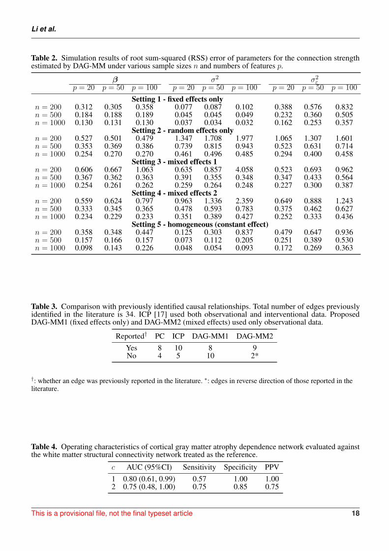
Table 2. Simulation results of root sum-squared (RSS) error of parameters for the connection strengthestimated by DAG-MM under various sample sizes n and numbers of features p.

� �

2�

2"

p = 20 p = 50 p = 100 p = 20 p = 50 p = 100 p = 20 p = 50 p = 100

Setting 1 - fixed effects onlyn = 200 0.312 0.305 0.358 0.077 0.087 0.102 0.388 0.576 0.832n = 500 0.184 0.188 0.189 0.045 0.045 0.049 0.232 0.360 0.505n = 1000 0.130 0.131 0.130 0.037 0.034 0.032 0.162 0.253 0.357

Setting 2 - random effects onlyn = 200 0.527 0.501 0.479 1.347 1.708 1.977 1.065 1.307 1.601n = 500 0.353 0.369 0.386 0.739 0.815 0.943 0.523 0.631 0.714n = 1000 0.254 0.270 0.270 0.461 0.496 0.485 0.294 0.400 0.458

Setting 3 - mixed effects 1n = 200 0.606 0.667 1.063 0.635 0.857 4.058 0.523 0.693 0.962n = 500 0.367 0.362 0.363 0.391 0.355 0.348 0.347 0.433 0.564n = 1000 0.254 0.261 0.262 0.259 0.264 0.248 0.227 0.300 0.387

Setting 4 - mixed effects 2n = 200 0.559 0.624 0.797 0.963 1.336 2.359 0.649 0.888 1.243n = 500 0.333 0.345 0.365 0.478 0.593 0.783 0.375 0.462 0.627n = 1000 0.234 0.229 0.233 0.351 0.389 0.427 0.252 0.333 0.436

Setting 5 - homogeneous (constant effect)n = 200 0.358 0.348 0.447 0.125 0.303 0.837 0.479 0.647 0.936n = 500 0.157 0.166 0.157 0.073 0.112 0.205 0.251 0.389 0.530n = 1000 0.098 0.143 0.226 0.048 0.054 0.093 0.172 0.269 0.363

Table 3. Comparison with previously identified causal relationships. Total number of edges previouslyidentified in the literature is 34. ICP [17] used both observational and interventional data. ProposedDAG-MM1 (fixed effects only) and DAG-MM2 (mixed effects) used only observational data.

Reported† PC ICP DAG-MM1 DAG-MM2Yes 8 10 8 9No 4 5 10 2*

†: whether an edge was previously reported in the literature. ⇤: edges in reverse direction of those reported in theliterature.

Table 4. Operating characteristics of cortical gray matter atrophy dependence network evaluated againstthe white matter structural connectivity network treated as the reference.

c AUC (95%CI) Sensitivity Specificity PPV1 0.80 (0.61, 0.99) 0.57 1.00 1.002 0.75 (0.48, 1.00) 0.75 0.85 0.75


Li et al.

Figure 1. Frequency of edges selected in 100 simulations. Edge width is proportional to the number oftimes an edge is identified in simulations. Black: true positive edges; Blue: false positive edges; Red: falsenegative edges (true edges that were never selected).

Li et al.

Figure 1. Frequency of edges selected in 100 simulations. Edge width is proportional to the number oftimes an edge is identified in simulations. Black: true positive edges; Blue: false positive edges; Red: falsenegative edges (true edges that were never selected).

DAG-MM PenPCSetting 1

1

2

3

4

5

6

7

89

10

11

12

13

14

15

Setting 1 - htDAG

1

2

3

4

5

6

7

89

10

11

12

13

14

15

Setting 1 - PenPC

Setting 2

1

2

3

4

5

6

7

89

10

11

12

13

14

15

Setting 2 - htDAG

1

2

3

4

5

6

7

89

10

11

12

13

14

15

Setting 2 - PenPC

Setting 3

1

2

3

4

5

6

7

89

10

11

12

13

14

15

Setting 3 - htDAG

1

2

3

4

5

6

7

89

10

11

12

13

14

15

Setting 3 - PenPC

Setting 4

1

2

3

4

5

6

7

89

10

11

12

13

14

15

Setting 4 - htDAG

1

2

3

4

5

6

7

89

10

11

12

13

14

15

Setting 4 - PenPC

Setting 5

1

2

3

4

5

6

7

89

10

11

12

13

14

15

Setting 5 - htDAG

1

2

3

4

5

6

7

89

10

11

12

13

14

15

Setting 5 - PenPC

This is a provisional file, not the final typeset article 18Frontiers 19

Li et al.

Figure 2. Estimated protein signaling network. Black: edges identified by DAG-MM2 and also reportedpreviously; Blue: edges are identified by DAG-MM2 but not reported previously; Gray: edges previouslyreported edges but not identified by DAG-MM2.

Figure 3. Estimated cortical thickness atrophy dependence network (organized into modules). The nodesize is proportional to the intra-modular connection strength (edge effects) and scaled within each subfigure.Red nodes: positive effects. Blue nodes: negative effects.

Li et al.

Figure 2. Estimated protein signaling network. Black: edges identified by DAG-MM2 and also reportedpreviously; Blue: edges are identified by DAG-MM2 but not reported previously; Gray: edges previouslyreported edges but not identified by DAG-MM2.

Figure 3. Estimated cortical thickness atrophy dependence network (organized into modules). The nodesize is proportional to the intra-modular connection strength (edge effects) and scaled within each subfigure.Red nodes: positive effects. Blue nodes: negative effects.

Population Average High versus Low Risk Older versus Younger

Frontiers 19This is a provisional file, not the final typeset article 20

Documents

Learning Directed Acyclic Graphs with Mixed Effects