1

Learning Deep Architectures for AI

Yoshua BengioDept. IRO, Universite de Montreal

C.P. 6128, Montreal, Qc, H3C 3J7, CanadaYoshua.Bengio@umontreal.ca

http://www.iro.umontreal.ca/∼bengioy

Technical Report 1312

Abstract

Theoretical results strongly suggest that in order to learnthe kind of complicated functions that can repre-sent high-level abstractions (e.g. in vision, language, and other AI-level tasks), one needsdeep architec-tures. Deep architectures are composed of multiple levels of non-linear operations, such as in neural netswith many hidden layers or in complicated propositional formulae re-using many sub-formulae. Searchingthe parameter space of deep architectures is a difficult optimization task, but learning algorithms such asthose for Deep Belief Networks have recently been proposed to tackle this problem with notable success,beating the state-of-the-art in certain areas. This paper discusses the motivations and principles regardinglearning algorithms for deep architectures, in particularthose exploiting as building blocks unsupervisedlearning of single-layer models such as Restricted Boltzmann Machines, used to construct deeper modelssuch as Deep Belief Networks.

1 Introduction

Allowing computers to model our world well enough to exhibitwhat we call intelligence has been the focusof more than half a century of research. To achieve this, it isclear that a large quantity of informationabout our world should somehow be stored, explicitly or implicitly, in the computer. Because it seemsdaunting to formalize manually all that information in a form that computers can use to answer questionsand generalize to new contexts, many researchers have turned to learning algorithmsto capture a largefraction of that information. Much progress has been made tounderstand and improve learning algorithms,but the challenge of artificial intelligence (AI) remains. Do we have algorithms that can understand scenesand describe them in natural language? Not really, except invery limited settings. Do we have algorithmsthat can infer enough semantic concepts to be able to interact with most humans using these concepts? No.If we consider image understanding, one of the best specifiedof the AI tasks, we realize that we do not yethave learning algorithms that can discover the many visual and semantic concepts that would seem to benecessary to interpret most images. The situation is similar for other AI tasks.We assume that the computational machinery necessary to express complex behaviors (which one mightlabel “intelligent”) requires highly varying mathematical functions, i.e. mathematical functions that arehighly non-linear in terms of raw sensory inputs. Consider for example the task of interpreting an inputimage such as the one in Figure 1. When humans try to solve a particular task in AI (such as machine visionor natural language processing), they often exploit their intuition about how to decompose the probleminto sub-problems and multiple levels of representation. Aplausible and common way to extract usefulinformation from a natural image involves transforming theraw pixel representation into gradually moreabstract representations, e.g., starting from the presence of edges, the detection of more complex but localshapes, up to the identification of abstract categories associated with sub-objects and objects which are parts

of the image, and putting all these together to capture enough understanding of the scene to answer questionsabout it. We view the raw input to the learning system as a highdimensional entity, made of many observedvariables, which are related by unknown intricate statistical relationships. For example, using knowledgeof the 3D geometry of solid object and lighting, we can relatesmall variations in underlying physical andgeometric factors (such as position, orientation, lighting of an object) with changes in pixel intensities forall the pixels in an image. In this case, our knowledge of the physical factors involved allows one to get apicture of the mathematical form of these dependencies, andof the shape of the set of images associatedwith the same 3D object. If a machine captured the factors that explain the statistical variations in the data,and how they interact to generate the kind of data we observe,we would be able to say that the machineunderstandsthose aspects of the world covered by these factors of variation. Unfortunately, in general andfor most factors of variation underlying natural images, wedo not have an analytical understanding of thesefactors of variation. We do not have enough formalized priorknowledge about the world to explain theobserved variety of images, even for such an apparently simple abstraction asMAN , illustrated in Figure 1.A high-level abstraction such asMAN has the property that it corresponds to a very large set of possibleimages, which might be very different from each other from the point of view of simple Euclidean distancein the space of pixel intensities. The set of images for whichthat label could be appropriate forms a highlyconvoluted region in pixel space that is not even necessarily a connected region. TheMAN category can beseen as a high-level abstraction with respect to the space ofimages. What we call abstraction here can be acategory (such as theMAN category) or afeature, a function of sensory data, which can be discrete (e.g., theinput sentence is at the past tense) or continuous (e.g., theinput video shows an object moving at a particularvelocity). Many lower level and intermediate level concepts (which we also call abstractions here) would beuseful to construct aMAN -detector. Lower level abstractions are more directly tiedto particular percepts,whereas higher level ones are what we call “more abstract” because their connection to actual percepts ismore remote, and through other, intermediate level abstractions.We do not know exactly how to build robustMAN detectors or even intermediate abstractions that wouldbe appropriate. Furthermore, the number of visual and semantic categories (such asMAN ) that we wouldlike an “intelligent” machine to capture is large. The focusof deep architecture learning is to automaticallydiscover such abstractions, from the lowest level featuresto the highest level concepts. Ideally, we would likelearning algorithms that enable this discovery with as little human effort as possible, i.e., without having tomanually define all necessary abstractions or having to provide a huge set of relevant hand-labeled examples.If these algorithms could tap into the huge resource of text and images on the web, it would certainly help totransfer much of human knowledge into machine-interpretable form.One of the important points we argue in the first part of this paper is that the functions learned should have astructure composed of multiple levels, analogous to the multiple levels of abstraction that humans naturallyenvision when they describe an aspect of their world. The arguments rest both on intuition and on theoreticalresults about the representational limitations of functions defined with an insufficient number of levels. Sincemost current work in machine learning is based on shallow architectures, these results suggest investigatinglearning algorithms for deep architectures, which is the subject of the second part of this paper.In much of machine vision systems, learning algorithms havebeen limited to specific parts of such a pro-cessing chain. The rest of of design remains labor-intensive, which might limit the scale of such systems.On the other hand, a hallmark of what we would consider intelligent includes a large enough vocabulary ofconcepts. RecognizingMAN is not enough. We need algorithms that can tackle a very largeset of suchtasks and concepts. It seems daunting to manually define thatmany tasks, and learning becomes essentialin this context. It would seem foolish not to exploit the underlying commonalities between these these tasksand between the concepts they require. This has been the focus of research onmulti-task learning(Caruana,1993; Baxter, 1995; Intrator & Edelman, 1996; Baxter, 1997). Architectures with multiple levels natu-rally provide such sharing and re-use of components: the low-level visual features (like edge detectors) andintermediate-level visual features (like object parts) that are useful to detectMAN are also useful for a largegroup of other visual tasks. In addition, learning about a large set of interrelated concepts might provide akey to the kind of broad generalizations that humans appear able to do, which we would not expect from

2

separately trained object detectors, with one detector pervisual category. If each high-level category is itselfrepresented through a particular configuration of abstractfeatures, generalization to unseen categories couldfollow naturally from new configurations of these features.Even though only some configurations of thesefeatures would be present in the training examples, if they represent different aspects of the data, new ex-amples could meaningfully be represented by new configurations of these features. This idea underlies theconcept ofdistributed representationthat is at the core of many of the learning algorithms described in thispaper, and discussed in Section 4.

Figure 1: We would like the raw input image to be transformed into gradually higher levels of representation,representing more and more abstract functions of the raw input, e.g., edges, local shapes, object parts, etc.In practice, we do not know in advance what the “right” representation should be for all these levels ofabstractions, although linguistic concepts might help us imagine what the higher levels might implicitlyrepresent.

This paper has two main parts which can be read almost independently. In the first part, Sections 2, 3and 4 use mathematical arguments to motivate deep architectures, in which each level is associated with adistributed representation of the input. The second part (in the remaining sections) covers current learningalgorithms for deep architectures, with a focus on Deep Belief Networks, and their component layer, theRestricted Boltzmann Machine.The next two sections of this paper review mathematical results that suggest limitations of many existinglearning algorithms. Two aspects of these limitations are considered: insufficientdepth of architectures, andlocality of estimators. To understand the notion ofdepth of architecture, one must introduce the notionof a set of computational elements. An example of such a set is the set of computations performedby an

3

artificial neuron. A function can be expressed by the composition of elements from this set, using a graphwhich formalizes this composition, with one node per computational element. Depth of architecture refersto the depth of that graph, i.e. the longest path from an inputnode to an output node. When the set ofcomputational elements is the set of computations an artificial neuron can make (depending on its param-eter values), depth corresponds to the number of layers in a neural network. Section 2 reviews theoreticalresults showing that an architecture with insufficient depth can require many more computational elements,potentially exponentially more (with respect to input size), than architectures whose depth is matched to thetask. This is detrimental for learning. Indeed, if a function represents a solution to the task with a very largebut shallow architecture (with many computational elements), a lot of training examples might be neededto tune each of these elements. We say that the expression of afunction iscompactwhen it has few com-putational elements, i.e. less degrees of freedom that can be tuned by learning. So for a fixed number oftraining examples, we would expect that compact representations of the target function would yield bettergeneralization.Connected to the depth question is the question of locality of estimators, discussed in Section 3. This isanother, more geometrically obvious, limitation of a largeclass of non-parametric learning algorithms: theyobtain good generalization for a new inputx by mostly exploiting training examples in the neighborhoodof x. For example, thek nearest neighbors of the test pointx, among the training examples, vote for theprediction atx. This locality issue is directly connected to the literature on thecurse of dimensionality, butthe results we cite show thatwhat matters for generalization is not dimensionality, butinstead the numberof “variations” of the function we wish to obtain after learning. For example, if the function representedby the model is piecewise-constant (e.g. decision trees), then the question that matters is the number ofpieces required to approximate properly the target function. There are connections between the number ofvariations and the input dimension: one can readily design families of target functions for which the numberof variations is exponential in the input dimension, such asthe parity function withd inputs.Section 4 suggests how deep architectures could be exploited to extract multiple levels ofdistributed rep-resentations, where the set of configurations of values at each level of thecomputation graph can be verylarge. This would allow us to compactly represent a complicated function of the input.In the remainder, the paper describes and analyses some of the algorithms that have been proposed to traindeep architectures.1 Many of these algorithms are based on theautoassociator: a simple unsupervised al-gorithm for learning a one-layer model that computes a distributed representation for its input (Rumelhart,Hinton, & Williams, 1986a; Bourlard & Kamp, 1988; Hinton & Zemel, 1994). We also discussconvo-lutional neural networks, the oldest successful example of deep architecture, specialized for vision andsignal processing tasks (LeCun, Boser, Denker, Henderson,Howard, Hubbard, & Jackel, 1989; LeCun, Bot-tou, Bengio, & Haffner, 1998b). Sections 9 and 10 are devotedto a family of more recently proposed learningalgorithms that have been very successful to train deep architectures: Deep Belief Networks (DBNs) (Hin-ton, Osindero, & Teh, 2006) and Stacked Autoassociators (Bengio, Lamblin, Popovici, & Larochelle, 2007;Ranzato, Poultney, Chopra, & LeCun, 2007). DBNs are based onRestricted Boltzmann Machines (RBMs)and the Contrastive Divergence algorithm (Hinton, 2002), introduced in Section 6. In Section 7 we describeestimators of the log-likelihood gradient for RBMs. This analysis shows how reconstruction error (usedto train autoassociators), and Contrastive Divergence (used to train RBMs) approximate the log-likelihoodgradient. Section 8 generalizes as much as possible the parametrization of RBMs so as to keep its basicfactorizing property and the Contrastive Divergence estimator of the gradient. Finally, we consider the mostchallenging question: how can we possibly deal with the difficult optimization problem that training thesedeep architectures entails? This part of the paper containsmostly questions and suggestions for researchdirections. In particular, we discuss the principle of continuation methods, which first solves smoother ver-sions of the desired cost function, to make a dent in the optimization of deep architectures, and we find thatexisting algorithms for RBMs and DBNs already are approximate continuation methods.

1Mostly deep neural networks, to date, but we suggest later that ensembles of trees could be learned and stacked similarlyto layersin a neural network.

4

1.1 Desiderata for Learning AI

Summarizing some of the above issues, we state a number of requirements we perceive for learning algo-rithms to solve AI.

• Ability to learn complex, highly-varying functions, i.e.,with a number of variations much greater thanthe number of training examples.

• Ability to learn with little human input the low-level, intermediate, and high-level abstractions thatwould be useful to represent the kind of complex functions needed for AI tasks.

• Ability to learn from a very large set of examples: computation time for training should scale wellwith the number of examples, i.e. close to linearly.

• Ability to learn from mostly unlabeled data, i.e. to work in the semi-supervised setting, where not allthe examples come with the “right” associated labels.

• Ability to exploit the synergies present across a large number of tasks, i.e. multi-task learning. Thesesynergies exist because all the AI tasks provide different views on the same underlying reality.

• In the limit of a large number of tasks and when future tasks are not known ahead of time, strongunsupervised learning(i.e. capturing the statistical structure in the observed data) is an importantelement of the solution.

Other elements are equally important but are not directly connected to the material in this paper. Theyinclude the ability to learn to represent context of varyinglength and structure (Pollack, 1990), so as toallow machines to operate in a stream of observations and produce a stream of actions, the ability to makedecisions when actions influence the future observations and future rewards (Sutton & Barto, 1998), and theability to influence future observations so as to collect more relevant information about the world (i.e. a formof active learning (Cohn, Ghahramani, & Jordan, 1995)).

2 Theoretical Limitations of Shallow Architectures

In this section, we present an argument in favor of deep architecture models by way of theoretical results re-vealing limitations of archictectures with insufficient depth. This part of the paper (this section and the next)motivate the algorithms described in the later sections, and can be skipped without making the remainderdifficult to follow. The main conclusion of this section is that functions that can be compactly representedby a depthk architecture might require an exponential number of computational elements to be representedby a depthk − 1 architecture. Since the number of computational elements one can afford depends on thenumber of training examples available to tune or select them, the consequences are not just computationalbut also statistical: poor generalization may be expected when using an insufficiently deep architecture forrepresenting some functions.We consider the case of fixed-dimension inputs, where the computation performed by the machine can berepresented by a directed acyclic graph where each node performs a computation that is the application ofa function on its inputs, each of which is the output of another node in the graph or one of the externalinputs to the graph. The whole graph can be viewed as acircuit that computes a function applied to theexternal inputs. When the set of functions allowed for the computation nodes is limited tologic gates, suchas{ AND, OR, NOT}, this is a boolean circuit, orlogic circuit .Let us return to the notion of depth with more examples of architectures of different depths. Consider thefunctionf(x) = x ∗ sin(a ∗ x + b). It can be expressed as the composition of simple operationssuch asaddition, subtraction, multiplication, and thesin operation, as illustrated in Figure 2. In the example, therewould be a different node for the multiplicationa ∗ x and for the final multiplication byx. Each node inthe graph is associated with an output value obtained by applying some function on input values that are

5

x

*

sin

+*

sin

+

neuron

neuron

neuron

neuron neuron neuron

neuron neuron

neuron setelement

...

inputs

output

*

b−

element set

output

inputs

a

Figure 2: Examples of functions represented by a graph of computations, where each node is taken insome set of allowed computations. Left: the elements are{∗, +, sin} ∪

�. The architecture computes

x∗sin(a∗x+b) and has depth 4. Right: the elements are artificial neurons computingf(x) = tanh(b+w′x);each element in the set has a different(w, b) parameter. The architecture is a multi-layer neural network ofdepth 3.

the outputs of other nodes of the graph. For example, in a logic circuit each node can compute a booleanfunction taken from a small set of boolean functions. The graph as a whole has input nodes and output nodesand computes a function from input to output. Thedepth of an architecture is the maximum length of a pathfrom any input of the graph to any output of the graph, i.e. 3 inthe case ofx ∗ sin(a ∗ x + b) in Figure 2.

• If we include affine operations and sigmoids in the set of computational elements, linear regressionand logistic regression have depth 1, i.e., have a single level.

• When we put a fixed kernel computationK(u, v) in the set of allowed operations, along with affineoperations, kernel machines (Scholkopf, Burges, & Smola,1999a) with a fixed kernel can be consid-ered to have two levels. The first level has one element computing K(x, xi) for each prototypexi (aselected representative training example) and matches theinput vectorx with the prototypesxi. Thesecond level performs a linear combination

∑i αiK(x, xi) to associate the matching prototypesxi

with the expected response.

• When we put artificial neurons (affine transformation followed by a non-linearity) in our set of el-ements, we obtain ordinary multi-layer neural networks (Rumelhart et al., 1986a). With the mostcommon choice of one hidden layer, they also have depth two (the hidden layer and the output layer).

• Decision trees can also be seen as having two levels, as discussed in Section 3.3.

• Boosting (Freund & Schapire, 1996) usually adds one level toits base learners: that level computes avote or linear combination of the outputs of the base learners.

• Stacking (Wolpert, 1992) is another meta-learning algorithm that adds one level.

• Based on current knowledge of brain anatomy (Serre, Kreiman, Kouh, Cadieu, Knoblich, & Poggio,2007), it appears that the cortex can be seen as a deep architecture, e.g., consider the many so-calledlayers in the visual system.

Although depth depends on the choice of the set of allowed computations for each element, theoreticalresults suggest that it is not the absolute number of levels that matters, but the number of levels relative tohow many are required to represent efficiently the target function (with some choice of set of computationalelements). As we will describe, if a function can be compactly represented withk levels using a particular

6

choice of computational element set, it might require a hugenumber of computational elements to representit with k − 1 or less levels (using that same computational element set).The most formal arguments about the power of deep architectures come from investigations into computa-tional complexity of circuits. The basic conclusion that these results suggest is thatwhen a function can becompactly represented by a deep architecture, it might needa very large architecture to be represented byan insufficiently deep one.A two-layer circuit of logic gates can represent any booleanfunction (Mendelson, 1997). Any booleanfunction can be written as a sum of products (disjunctive normal form: AND gates on the first layer withoptional negation of inputs, and OR gate on the second layer)or a product of sums (conjunctive normalform: OR gates on the first layer with optional negation of inputs, and AND gate on the second layer). Tounderstand the limitations of shallow architectures, the first important result to consider is that with depth-two logical circuits, most boolean functions require anexponentialnumber of logic gates (Wegener, 1987)to be represented (with respect to input size).Furthermore, there are functions computable with a polynomial-size logic gates circuit of depthk that requireexponential size when restricted to depthk − 1 (Hastad, 1986). The proof of this theorem relies on earlierresults (Yao, 1985) showing thatd-bit parity circuits of depth 2 have exponential size. The d-bit parityfunction is defined as usual:

parity : (b1, . . . , bd) ∈ {0, 1}d 7→

{1 if

∑di=1 bi is even

−1 otherwise.

One might wonder whether these computational complexity results for boolean circuits are relevant to ma-chine learning. See Orponen (1994) for an early survey of theoretical results in computational complexityrelevant to learning algorithms. Interestingly, many of the results for boolean circuits can be generalizedto architectures whose computational elements arelinear threshold units (also known as artificial neu-rons (McCulloch & Pitts, 1943)), which compute

f(x) = �w′x+b≥0 (1)

with parametersw andb. Thefan-in of a circuit is the maximum number of inputs of a particular element.Circuits are often organized in layers, like multi-layer neural networks, where elements in a layer only taketheir input from elements in the previous layer(s), and the first layer is the neural network input. Thesizeofa circuit is the number of its computational elements (excluding input elements, which do not perform anycomputation).One might argue that the limitations of logic gates circuitsmight not apply to the kind of architecturesfound in machine learning algorithms. With that in mind, it is interesting to note that similar theorems wereproved for circuits of linear threshold units, which are thecomputational elements of some multi-layer neuralnetworks. Of particular interest is the following theorem,which applies tomonotone weighted thresholdcircuits (i.e. multi-layer neural networks with linear threshold units and positive weights) when trying torepresent a function compactly representable with a depthk circuit:

Theorem 2.1. A monotone weighted threshold circuit of depthk − 1 computing a functionfk ∈ Fk,N hassize at least2cN for some constantc > 0 andN > N0 (Hastad & Goldmann, 1991).

The class of functionsFk,N is defined as follows. It contains functions ofN2k−2 variables each defined bya depthk circuit that is a tree. At the leaves of the tree there are unnegated input variables, and the functionvalue is at the root. Thei-th level from the bottom consists of AND gates wheni is even and OR gates wheni is odd. The fan-in at the top and bottom level isN and at all other levels it isN2.The above results do not prove that other classes of functions (such as those we want to learn to performAI tasks) require deep architectures, nor that these demonstrated limitations apply to other types of circuits.However, these theoretical results beg the question: are the depth 1, 2 and 3 architectures (typically foundin most machine learning algorithms) too shallow to represent efficiently more complicated functions? Re-sults such as the above theorem also suggest thatthere might be no universally right depth: each function

7

(i.e. each task) might require a particular minimum depth (for a given set of computational elements). Weshould therefore strive to develop learning algorithms that use the data to determine the depth of the finalarchitecture.Depth of architecture is connected to the notion of highly-varying functions. We argue that, in general, deeparchitectures can compactly represent highly-varying functions which would otherwise require a very largesize to be represented with an inappropriate architecture.We say that a function ishighly-varying whena piecewise approximation (e.g., piecewise-constant or piecewise-linear) of that function would require alarge number of pieces. A deep architecture is a compositionof many operations, and it could in any casebe represented by a possibly very large depth-2 architecture. The composition of computational units in asmall but deep circuit can actually be seen as an efficient factorization of a large but shallow circuit. Reor-ganizing the way in which computational units are composed can have a drastic effect on the efficiency ofrepresentation size. For example, whereas the polynomial

∏ni=1

∑mj=1 aijxj can be represented efficiently

as a product of sums, with onlyO(mn) computational elements, it would be very inefficiently representedwith a sum of product architecture, requiringO(nm) computational elements.Further examples suggesting greater expressive power of deep architectures and their potential for AI andmachine learning are also discussed in Bengio and Le Cun (2007). An earlier discussion of the expectedadvantages of deeper architectures in a more cognitive perspective is found in Utgoff and Stracuzzi (2002).Having established some theoretical grounds justifying the need for learning deep architectures, we next turnto a related question: deep architectures can represent highly-varying functions compactly, with less com-putational elements than there are variations in the represented function, but many state-of-the-art machinelearning algorithms do not have that characteristic.To conclude, a number of computational complexity results strongly suggest that functions that can be com-pactly represented with a depthk architecture could require a very large number of elements in order to berepresented by a shallower architecture. Since each element of the architecture might have to be selected,i.e., learned, using examples, these results mean that depth of architecture can be very important from thepoint of view a statistical efficiency.

3 Local vs Non-Local Generalization: the Limits of Matching LocalTemplates

This section focuses on the locality of estimators in many shallow architectures, which gives rise to poorgeneralization when trying to learn highly-varying functions. This is because highly-varying functions,which can sometimes be represented efficiently with deep architectures, cannot be represented efficiently ifthe learning algorithm is a local estimator.A local estimatorpartitions the input space in regions (possibly in a soft rather than hard way) and requiresdifferent parameters or degrees of freedom to account for the possible shape of the target function in each ofthe regions. When many regions are necessary because the function is highly varying, the number of requiredparameters will also be large, and thus the number of examples needed to achieve good generalization.As an extreme example of a shallow and local architecture, consider a disjunctive normal form (depth 2)logic-gate circuit with all possible2n gates at the first level. The2n possibilities come from the choice, foreach gate, of negating or not each of then inputs before applying the AND computation. Each such productis called aminterm . One can see such as circuit simply as a very large pattern matcher. More generally, ifonly a subset of the input variables is used in a particular AND gate, then that gate will respond to a largerset of input patterns. The gate is then a template matcher that responds to patterns in a connected region ofinput space, e.g. the subspace that is the set of vectorsx such thatx1 = 1, x2 = 0 but x3 andx4 can takeany value.More generally, architectures based on matching local templates can be thought of as having two levels. Thefirst level is made of a set of templates which can be matched tothe input. A template unit will output avalue that indicates the degree of matching. The second level combines these values, typically with a simple

8

linear combination (an OR-like operation), in order to estimate the desired output. The prototypical exampleof architectures based on maching local templates is thekernel machine(Scholkopf et al., 1999a)

f(x) = b +∑

i

αiK(x, xi), (2)

whereb andαi form the second level,kernel function K(x, xi) matches the inputx to the training examplexi, and the sum runs over all or a subset of the input patterns of the training set. In the above equation,f(x)could be the discriminant function of a classifier, or the output of regression predictor. A kernel islocal, whenK(x, xi) > ρ is true forx in some connected region aroundxi. The size of that region can usually be con-trolled by a hyper-parameter. An example of local kernel is the Gaussian kernelK(x, xi) = e−||x−xi||

2/σ2

,whereσ controls the size of the region aroundxi. We can see the Gaussian kernel as computing a soft con-junction, because it can be written as a product of one-dimensional conditions:K(u, v) =

∏i e−(ui−vi)

2/σ2

.If |ui − vi|/σ is small for alli, then the pattern matches andK(u, v) is large. If |ui − vi|/σ is large for asinglei, then there is no match andK(u, v) is small.Well-known example of kernel machines include Support Vector Machines (SVMs) (Boser, Guyon, & Vap-nik, 1992; Cortes & Vapnik, 1995) and Gaussian processes (Williams & Rasmussen, 1996)2 for classifica-tion and regression, but also classical non-parametric learning algorithms for classification, regression anddensity estimation, such as thek-nearest neighbor algorithm, Nadaraya-Watson or Parzen windows densityand regression estimators, etc. In Section 3.2 we discussmanifold learning algorithmssuch as Isomap andLLE that can also be seen as local kernel machines, as well as related semi-supervised learning algorithmsalso based on the construction of aneighborhood graph (with one node per example and arcs betweenneighboring examples).Kernel machines with a local kernel yield generalization byexploiting what could be called thesmoothnessprior : the assumption that the target function is smooth or can be well approximated with a smooth function.For example, in supervised learning, if we have the trainingexample(xi, yi), then it makes sense to constructa predictorf(x) which will output something close toyi whenx is close toxi. Note how this prior requiresdefining a notion of proximity in input space. This is a usefulprior, but one of the claims made in Bengio,Delalleau, and Le Roux (2006) and Bengio and Le Cun (2007) is that such a prior if often insufficient togeneralize when the target function is highly-varying in input space (according to the notion of proximityembedded in the prior or kernel). Consider that most kernelsused in practice can be seen as a dot product ina feature space:K(x, xi) = φ(x) · φ(xi), where generallyφ(x) is a non-linear transformation of the inputx into a high-dimensionalfeature space. A good feature space would be one where the target function issmooth when expressed in the feature space. One could therefore correctly argue that if the target function ishighly varying in input space and in the kernel feature space, it might simply be because we have not selectedthe appropriate feature space. If our feature space does nothave that property, i.e. the approximationy ≈ yi

whenφ(x) ≈ φ(xi) is only valid in a small region aroundφ(xi), then one will need many such regions tocover the domain of interest. Unfortunately, at least as many training examples will be needed as there areregions necessary to cover the variations of interest in thetarget function.The limitations of a fixed generic kernel such as the Gaussiankernel have motivated a lot of research indesigning kernelsbased on prior knowledge about the task (Jaakkola & Haussler, 1998; Scholkopf, Mika,Burges, Knirsch, Muller, Ratsch, & Smola, 1999b; Gartner, 2003; Cortes, Haffner, & Mohri, 2004). How-ever, if we lack sufficient prior knowledge for designing an appropriate kernel, can we learn it? this ques-tion also motivated much research (Lanckriet, Cristianini, Bartlett, El Gahoui, & Jordan, 2002; Wang &Luk Chan, 2002; Cristianini, Shawe-Taylor, Elisseeff, & Kandola, 2002), and deep architectures can beviewed as a promising development in this direction. It has been shown that a Gaussian Process kernelmachine can be improved using a Deep Belief Network to learn afeature space (Salakhutdinov & Hinton,2008): predictions are improved by using the top-level representation instead of the raw input representa-tion, and they are further improved by tuning the deep network to minimize the prediction error made by

2In the Gaussian Process case, as in kernel regression,f(x) in eq. 2 is the conditional expectation of the target variableY to predict,given the inputx

9

the Gaussian process, using gradients of the prediction error back-propagated into the neural network. Thefeature space can be seen as a representation of the data. Good representations make examples which shareabstract characteristics close to each other. Learning algorithms for deep architectures can be seen as waysto learn a good feature space for kernel machines.In the next subsection we review theoretical results on the limitations of kernel machines with a Gaussiankernel in the case of supervised learning, which show that the required number of examples grows linearlywith the number of bumps in the target function to be learned.In subsection 3.2 we present results of asimilar flavor for semi-supervised non-parametric learning algorithms, and in subsection 3.3 for decisiontrees. We conclude in subsection 3.4 with a discussion on theuse of smoothness as a prior, and how itcan be made more powerful by extending the notion of complexity of a function, in the extreme case usingKolmogorov complexity.

3.1 Theoretical Limitations of Local Kernels

Here we consider formal results about limitations of local kernel machines. The notion that local kernelsare insufficient to capture highly-varying functions is formalized in a few particular cases in Bengio et al.(2006), Bengio and Le Cun (2007). One result is the following:

Theorem 3.1. Suppose that the learning problem is such that in order to achieve with a Gaussian kernelmachine (eq. 2) a given error level for samples from a distributionP , f must change sign at least2k timesalong some straight line (i.e., in the case of a classifier, a sufficiently good decision surface must be crossedat least2k times by that straight line). Then the kernel machine must have at leastk bases (non-zeroαi’s),and hence at leastk training examples.

decision surface

Class −1

Class 1

Figure 3: The dotted line crosses the decision surface 19 times: according to Theorem 3.1, and in line withintuition, one needs 10 Gaussians to learn it with an affine combination of Gaussians, with each Gaussiancapturing one of the bumps in the function.

This theorem says that we need as many examples as there are variations (“bumps”) in the function thatwe wish to represent with a Gaussian kernel machine. As illustrated in Figure 3, a function may have a

10

large number of variations (e.g. a sinusoidal) and yet be representable much more compactly because thesevariations are interdependent. It is conceivable that a different learning algorithm could take advantage ofthe global regularity (repeating pattern) to learn it with few parameters (thus requiring few examples). Bycontrast, with an affine combination of Gaussians, theorem 3.1 implies one would need at leastdm

2 e = 10Gaussians. With a local estimator, it is plausible that moreexamples will be needed to take care of newinstances of the repeating pattern in the curve. For complextasks in high dimension, the complexity of thedecision surface could quickly make learning impractical when using a local kernel method. It could alsobe argued that if the curve has many variations and these variations are not related to each other throughan underlying regularity, then no learning algorithm will do much better than local estimators. However,it might be worth it to look for more compact representationsof these variations, because if one could befound, it would be likely to lead to better generalization, especially for variations not seen in the training set.Of course this could only happen if there were underlying regularities to be captured in the target function,but these are the functions that we want to learn for AI.A different type of variability is illustrated by the parityfunction, where a small change in any direction ininput space corresponds to a large change in the desired output. In that case one can show (Bengio et al.,2006) that the number of examples necessary with a Gaussian kernel machine is exponential in the inputdimension:

Theorem 3.2. Let f(x) = b +∑2d

i=1 αiKσ(xi, x) be an affine combination of Gaussians with same widthσ centered on pointsxi ∈ {−1, 1}d. If f solves the parity problem, then there are at least2d−1 non-zerocoefficientsαi.

Note that one way in which the parity function is not representative of the kind of functions we are moreinterested in AI is that the target function does not depend on the order of the inputs. Also, parity can berepresented with a shallow neural network withO(d) units (andO(d2) parameters). This solution exploitsthe fact that projecting the input vectorx to the scalars =

∑i xi preserves the information that is necessary

to compute parity: it is enough to consider in which ofd+1 intervalss falls to determine the correct answer,andd threshold units are sufficient to achieve this.Hence the theoretical results discussed in this section aremerely suggestive but do not prove that the learningalgorithms for the functions that we need to represent for AIshould not be local estimators.

3.2 Unsupervised and Semi-Supervised Algorithms Based on Neighborhood-Graph

Local estimators are found not only in supervised learning algorithms such as those discussed above, but alsoin unsupervised and semi-supervised learning algorithms,to which we now turn. Here again, we find that inorder to cover the many possible variations in the function to be learned, one needs a number of examplesproportional to the number of variations to be covered.Unsupervised learningalgorithms attempt to capture characteristics of the inputdistribution. For exam-ple, manifold learning algorithms attempt to discover a lower-dimensional regionnear which the densityconcentrates. There is a connection between kernel machines such as SVMs and Gaussian processes anda number of unsupervised and semi-supervised learning algorithms: many of these unsupervised and semi-supervised algorithms can be expressed as kernel machines with a particular kernel, one that is possiblydata-dependent (Bengio, Delalleau, Le Roux, Paiement, Vincent, & Ouimet, 2004). The following unsuper-vised learning algorithms, included in this analysis, attempt to capture the manifold structure of the data bycapturing its local changes in shape: Locally Linear Embedding (Roweis & Saul, 2000), Isomap (Tenen-baum, de Silva, & Langford, 2000), kernel Principal Components Analysis (Scholkopf, Smola, & Muller,1998) (or kernel PCA) Laplacian Eigenmaps (Belkin & Niyogi,2003), Manifold Charting (Brand, 2003),and spectral clustering algorithms (see Weiss (1999) for a review). Several non-parametric semi-supervisedlearning algorithms are based on similar concepts, involving the use of a kernel (Zhu, Ghahramani, & Laf-ferty, 2003; Zhou, Bousquet, Navin Lal, Weston, & Scholkopf, 2004; Belkin, Matveeva, & Niyogi, 2004;Delalleau, Bengio, & Le Roux, 2005).

11

Most of these unsupervised and semi-supervised algorithmsrely on theneighborhood graph: a graph withone node per example and arcs between near neighbors. The question we want to discuss here is whether theabove non-parametric algorithms are likely to suffer from the same limitations already discussed for localkernel machines for classification or regression in the previous section. With these algorithms, one can getgeometric intuition of what they are doing, as well as how being a local estimators can hinder them. Thisis illustrated with the example in Figure 4 in the case of manifold learning. The issue is related to the curseof dimensionality: to cover all the variations with locallylinear patches, a lot of patches might be necessary,and enough examples in each patch to characterize its shape,i.e. the tangent plane at the patch location.

Figure 4: The set of images associated with the same object class forms a manifold, i.e. a region of lowerdimension than the original space of images. By rotating, translating, or shrinking an image, e.g., of digit 4,we get other images of the same class, i.e. on the same manifold. Since the manifold is locally smooth, it canin principle be approximated locally by linear patches, each being tangent to the manifold. Unfortunately, ifthe manifold is highly curved, the patches are required to besmall, and exponentially many might be neededwith respect to manifold dimension.

Similar limitations have been proved for a large class of semi-supervised learning algorithms also based onthe neighborhoodgraph (Zhu et al., 2003; Zhou et al., 2004; Belkin et al., 2004; Delalleau et al., 2005). Thesealgorithms partition the neighborhood graph in regions of constant label. It can be shown that the numberof regions with constant label cannot be greater than the number of labeled examples (Bengio et al., 2006).Hence one needs at least as many labeled examples as there arevariations of interest for the classification.This can be prohibitive if the decision surface of interest has a very large number of variations.

3.3 Decision Trees Do not Generalize to New Variations

Decision trees are among the best studied learning algorithms. Because they can focus on specific subsetsof input variables, at first blush they seem non-local. However, they are also local estimators in the sense ofrelying on a partition of the input space and using separate parameters for each region (Bengio, Delalleau,& Simard, 2007). As we argue here, this means that they also suffer from the limitation discussed for othernon-parametric learning algorithms in the previous sections: they need at least as many training examples asthere are variations of interest in the target function, andthey cannot generalize to new variations not coveredin the training set.As illustrated in Figure 5, a decision tree recursively partitions the input space and assigns an output valuefor each of the input regions in that partition. Learning algorithms for decision trees (Breiman, Friedman,Olshen, & Stone, 1984) are non-parametric and involve a non-convex optimization to choose a tree structureand parameters associated with nodes and leaves. Fortunately, greedy heuristics that build the tree incre-mentally have been found to work well. Each node of the tree corresponds to a region of the input space,

12

x1<2

x2<1

x1<0.5 x1<1.25

R1

R2 R3 R4 R5

x1

x2

2

R11

R2

.5

R3

R4

R5

1.25

Figure 5: A decision tree recursively partitions the input space. In a binary tree, the root node splits it in two.Each node is associated with a region. An output value is learned for each leaf node region.

and the root is associated with the whole input space. We callconstant-leaves decision tree(the commontype) one where the whole tree corresponds to a piece-wise constant function where the pieces are definedby the internal decision nodes: each leaf is associated withone piece, along with a constant to output inthe associated region. The decision nodes on the path from the root to a leaf define one of the mutuallyexclusive regions formed by the decision tree. Like in a disjunctive normal form circuit or a Gaussian kernelmachine, the outputs of decision nodes are multiplied and form a conjunction: an example has to satisfy allthe conditions to belong to a leaf region. The decision nodesform the first level of the architecture. Thepredictions associated with the leaves, along with their parameters, form the second level of the architecture.Bengio et al. (2007) study fundamental limitations of decision trees concerning their inability togeneralizeto variations not seen in the training set. The basic argument is that a decision tree needs a separate leafnode to properly model each such variation, and at least one training example for each leaf node. Thattheoretical analysis is built along lines similar to ideas exploited previously in the computational complexityliterature (Cucker & Grigoriev, 1999). These results are also in line with previous empirical results (Perez& Rendell, 1996; Vilalta, Blix, & Rendell, 1997) showing that the generalization performance of decisiontrees degrades when the number of variations in the target function increases.The following results are taken from Bengio et al. (2007).

Proposition 3.3. LetF be the set of piece-wise constant functions. Consider a target functionh :�d →

�. For a given representation error levelε, let N be the minimum number of constant pieces required to

approximate, with a function inF , the target functionh with an error less thanε. Then to train a constant-leaves decision tree with error less thanε one requires at leastN training examples.

The above proposition states that the number of examples needed grows linearly with the number of regionsneeded to achieve a desired error level. The theorem below states a more specific result in the case of afamily of function for which the number of needed regions is exponential in the input size.

13

C2=0C3=0

C1=1

C2=1C3=0

C1=0

C2=0C3=0

C1=0

C2=1C3=1

C1=0

Partition 3Partition 2

Partition 1

Figure 6: Whereas a single tree can discriminate among a number of regions linear in the number of parame-ters (leaves), an ensemble of trees can discriminate among anumber of regions exponential in the number oftrees, i.e. exponential in the total number of parameters (at least as long as the number of trees is less or equalto the number of inputs). Each distinguishable region is associated with one of the leaves of each tree (herethere are 3 trees, each defining 2 regions, for a total of 7 regions). This is equivalent to a multi-clustering,here 3 clusterings each associated with 2 regions. A binomial RBM is a multi-clustering with 2 linearlyseparated regions per partition (each associated with one hidden unit). A multi-clustering is therefore adistributed representation of the input pattern.

Theorem 3.4. On the task of learning thed-bit parity function, a constant-leaves decision tree withaxis-aligned decision nodes will require at least2d(1 − 2ε) examples in order to achieve a generalization errorless than or equal toε.

Ensembles of trees (like boosted trees (Freund & Schapire, 1996), and forests (Ho, 1995; Breiman, 2001))are more powerful than a single tree. They add a third level tothe architecture which allows the model todiscriminate among a number of regionsexponential in the number of parameters(Bengio et al., 2007).As illustrated in Figure 6, they implicitly form adistributed representation(a notion discussed further inSection 4) with the output of all the trees in the forest. Eachtree in an ensemble can be associated with adiscrete symbol identifying the leaf/region in which the input example falls for that tree. The description ofan input pattern with the identities of the leaf nodes for thetrees is very rich: it can represent a very largenumber of possible patterns, because the number of intersections of the leaf regions associated with thentrees can be exponential inn. Since a depthk − 1 architecture might be very inefficient to represent a depthk function, it might be interesting to explore learning algorithms based upon decision trees in which thearchitecture depth is even greater than in ensembles of trees.

3.4 Smoothness versus Kolmogorov Complexity

To escape the curse of dimensionality, it is necessary to have a model that can capture a large number ofvariations that can occur in the data without having to enumerate all of them. Instead, a compact representa-tion that captures most of these variations has to be discovered by the learning algorithm. Here “compact”means that itcould beencoded with a few bits.The notion of local estimator is connected to the notion of smoothness and smoothness priors introducedat the beginning of Section 3. Smoothness as a measure of simplicity is a useful way to control general-ization, but others are possible, and probably more desirable. For example, consider a target function ishighly-varying with a number of variations much larger thanthe number of training examples one can hopeto get. A deep architecture could potentially represent such a function with a small number of parameters(comparable to the number of training examples one could get). If one discovers such a compact represen-tation of the target function, then a form of compression hasbeen achieved. This is likely to yield good

14

generalization (Solomonoff, 1964; Kolmogorov, 1965; Li & Vitanyi, 1997; Hutter, 2005) because of Oc-cam’s Razor. Maybe the most extreme and general way to measure that compression is with Kolmogorovcomplexity. TheKolmogorov complexity is the length of the smallest string that represents the solution, insome programming language. Using a different language onlyadds a constant to the string length (for thecode that translates strings in one language to strings in another). It is clear that many functions expressiblewith a very short string can be highly varying, such as the sinus example of Figure 3. Learning theory (Vap-nik, 1995; Li & Vitanyi, 1997) shows that if a compact description can be found to summarize the trainingset, good generalization is to be expected.The main advantage of smoothness expressed through a kernelor covariance function (in Gaussian pro-cesses) is that the optimization problem involved in the learning algorithm can be convex, i.e. devoid of lo-cal minima and hence easy to solve. Kolmogorov complexity isnot even computable, but it can be boundedfrom above. Upper bounds on Kolmogorov complexity can be optimized. Our thesis is that deep archi-tectures can represent many functions compactly, and that their approximate optimization might yield verygood solutions even if the global optimum is not found: any solution that is more compact than previousones brings a gain in generalization. Minimum Description Length (Rissanen, 1990) and its variants suchas Minimum Message Length (Wallace & Boulton, 1968) also usethis principle in the context of randomvariables with many realizations: a good predictive model (in terms of out-of-sample log-likelihood) is alsoone that can assign a short code to each example,on average, including not only the bits to describe eachexample but also the bits necessary to describe the model itself.What can be concluded from our analysis of limitations of learning algorithms due to insufficient depthand local estimation? In either case, insufficient depth or local estimator, we found that one might need torepresent the target function with a very large number of tunable elements, and thus one would need a verylarge number of examples. On the other hand, if a representation exists that can compactly represent thetarget function, then good generalization could be obtained from a number of examples much smaller thanthe number of variations of the target function. An important idea that gives hope of compactly representinga very large number of configurations is the idea of distributed representation, discussed next, and whichintroduces the second part of this paper, about learning algorithms for deep architectures.

4 Learning Distributed Representations

An old idea in machine learning and neural networks research, which could be of help in dealing withthe curse of dimensionality and the limitations of local generalization is that ofdistributed representa-tions (Hinton, 1986; Rumelhart, McClelland, & the PDP Research Group, 1986b; Bengio, Ducharme, &Vincent, 2001). A cartoonlocal representationfor integersi ∈ {1, 2, . . . , N} is a vectorr(i) of N bitswith a single 1 andN − 1 zeros,rj(i) = �i=j , called theone-hotrepresentation ofi. A distributed repre-sentation for the same integer is a vector oflog2 N bits, which is a much more compact way to representi.For the same number of possible configurations, a distributed representation can potentially be exponentiallymore compact than a very local one. In practice, we use local representations which are continuous-valuedvectors where thei-th element varies according to some distance between the input and a prototype or re-gion center, as with the Gaussian kernel discussed in Section 3. In a distributed representation the inputpattern is represented by a set of features that are not mutually exclusive, and might even be statisticallyindependent. For example, clustering algorithms do not build a distributed representation since the clustersare essentially mutually exclusive, whereas Independent Components Analysis (Bell & Sejnowski, 1995;Pearlmutter & Parra, 1996) and Principal Components Analysis or PCA (Hotelling, 1933) build a distributedrepresentation.Consider a discrete distributed representationr(x) for an input patternx, whereri(x) ∈ {0, 1, . . .M},i ∈ {1, . . . , N}. Eachri(x) can be seen as a classification ofx into M classes. Eachri(x) partitions thex-space inM regions, but the different partitions can be combined to give rise to a potentially exponentialnumber of possible regions inx-space, corresponding to different configurations ofri(x). Note that someconfigurations may be impossible because they are incompatible. For example, in language modeling, a local

15

representation of a word could directly encode its identityby an index in the vocabulary table, or equivalentlya one-hot code with as many entries as the vocabulary size. Onthe other hand, a distributed representationcould represent the word by a number of syntactic features (e.g., distribution over parts of speech it canhave), morphological features (which suffix or prefix does ithave?), and semantic features (is it the name ofa kind of animal?). Like in clustering, we construct discrete classes, but the potential number of combinedclasses is huge: we obtain what we call amulti-clustering . Whereas clustering forms a single partitionand generally involves a loss of information about the input, a multi-clustering provides asetof separatepartitions of the input space. Identifying to which region of each partition the input example belongs formsa description of the input pattern which might be very rich, possibly not losing any information. The tupleof symbols specifying to which region of each partition the input belongs can be seen as a transformation ofthe input into a new space, where the statistical structure of the data and the factors of variation in it couldbe disentangled. This corresponds to the kind of partition of x-space that an ensemble of trees can represent,as discussed in the previous section.In the realm of supervised learning, multi-layer neural networks (Rumelhart et al., 1986b, 1986a) and Boltz-mann machines (Ackley, Hinton, & Sejnowski, 1985) have beenintroduced with the goal of learning dis-tributed internal representations in the hidden layers. Unlike in the linguistic example above, the objectiveis to let learning algorithms discover the features that compose the distributed representation. In a multi-layer neural network with more than one hidden layer, there are several representations, one at each layer.Learning multiple levels of distributed representations involves a challenging optimization problem, whichis central in the remainder of this paper.

5 Learning Deep Architectures: a Difficult Optimization Problem

After having motivated the need for deep architectures thatare non-local estimators, we now turn to thedifficult problem of training them. Experimental evidence suggests that training deep architectures involvesoptimization problems that are more difficult than those involved in training shallow architectures (Bengioet al., 2007). Much of that evidence comes from research on training multi-layer neural networks, suggestingthat training gets stuck in local minima or plateaus, with worse results than with neural networks with oneor two hidden layers.A typical set of equations for multi-layer neural networks is the following. As illustrated in Figure 7, layer` computes an output vectorz` using the outputz`−1 of the previous layer, starting with the inputz0,

z` = tanh(b` + W`z`−1) (3)

with parametersb` (the biases) andW` (the weights). Thetanh can be replaced bysigm(x) = 1/(1+e−x) =12 (tanh(x) + 1). The top layer outputzL is used for making a prediction and is combined with a supervisedtargety into a loss functionL(zL, y), typically convex. The output layer might have a non-linearity differentfrom tanh, e.g., the softmax

zLi =ebLi+WLizL−1

∑j ebLj+WLjzL−1

(4)

whereWLi is thei-th row of WL, zLi is positive and∑

i zLi = 1. The softmax outputzLi can be used asestimator ofP (Y = i|x), with the interpretation thatY = i is thei-th class associated with input patternx. In this case one often uses the negative conditional log-likelihoodL(zL, y) = − log zLy as a loss, whoseexpected value over(x, y) pairs is to be minimized.Deep architectures have not been studied much in the machinelearning literature, because of the difficulty inoptimizing them (Bengio et al., 2007). Notable exceptions includeconvolutional neural networks (LeCunet al., 1989; LeCun et al., 1998b; Simard & Platt, 2003; Ranzato et al., 2007), and Sigmoidal Belief Networksusing variational approximations (Dayan, Hinton, Neal, & Zemel, 1995; Hinton, Dayan, Frey, & Neal, 1995;Saul, Jaakkola, & Jordan, 1996; Titov & Henderson, 2007), and more recently Deep Belief Networks (Hintonet al., 2006; Bengio et al., 2007). Many unreported negativeobservations as well as the experimental results

16

Figure 7: Multi-layer neural network, typically used in supervised learning to make a prediction or classifica-tion, through a series of layers each of which combines an affine operation and a non-linearity. Computationsare performed in a feedforward way from the inputx, through the hidden layershk, to the network outputy,which gets compared with a labely to obtain the lossL(y, y) to be minimized.

in Bengio et al. (2007) suggest that gradient-based training of deep supervised multi-layer neural networksgets stuck in local minima or plateaus. These appear to correspond to poor solutions that perform worse thanthe solutions obtained for networks with 1 or 2 hidden layers. The experiments reported in Bengio et al.(2007) also help to disantangle the effect of poor optimization with the effect of overfitting. They revealthat in a gradient-trained deep supervised neural network with random parameter initialization, the lowerlayers (closer to inputs) are poorly optimized. Indeed, we know that a two-layer network can be well trainedin general, and that from the point of view of the top two layers in a deep network, they form a shallownetwork whose input is the output of the lower layers. If the top layers have enough capacity (enough hiddenunits) this can be sufficient to bring training error very low, but this yields worse generalization than shallowneural networks. On the other hand, with better initialization of the lower hidden layers, both trainingand generalization error can be very low. In a well-trained deep neural network, the hidden layers form a“good” representation of the data, which helps to make good predictions. When the lower layers are poorlyinitialized, these deterministic and continuous representations generally keep most of the information aboutthe input, but these representations might hurt rather thanhelp the top layers to perform classification. It issimple to obtain very smalltraining error by simply increasing the capacity of the top layer(s). For example,optimizing the last layer of a deep neural network is usuallya convex optimization problem. Optimizing thelast two layers, although not convex, is known to be much easier than optimizing a deep network. Hence,what matters for good generalization, and is more difficult,is the optimization of the lower layers (excludingthe last one or two). These are the layers that can give rise toa good representation of the input, in the sensethat better generalization can be achieved from these representations. We believe that good representationscapture the factors of variation in the input space and also disentangle them.Although replacing the top two layers of a deep neural network by a convex machine such as a Gaussianprocess or an SVM can yield some improvements (Bengio & Le Cun, 2007), especially on the training error,it won’t help much in terms of generalization if the lower layers have not been sufficiently optimized.The above clues suggest that the gradient propagated backwards into the lower layer is not sufficient tomove the parameters into regions corresponding to good solutions. Basically the optimization gets stuckin a poor local minimum or plateau (i.e. small gradient). Since gradient-based training of the top layersworks reasonably well, it appears that the gradient becomesless informative about the required changesin the parameters as we move towards the lower layers. There might be some connection between this

17

difficulty in exploiting the gradient and the difficulty in training recurrent neural networks through longsequences, analyzed in (Hochreiter, 1991; Bengio, Simard,& Frasconi, 1994; Lin, Horne, Tino, & Giles,1995). In recurrent neural networks, the difficulty can be traced to a vanishing (or sometimes explosion)of the gradient propagated through many non-linearities. There is an additional difficulty in the case ofrecurrent neural networks, due to a mismatch between short-term and long-term components of the gradient.

5.1 Convolutional Neural Networks

Although deep neural networks were generally found too difficult to train well, there is one notable excep-tion: convolutional neural networks. Convolutional nets were inspired by the visual system’s structure, andin particular by the models of it proposed by Hubel and Wiesel(1962). The first computational models basedon these local connectivities between neurons and on hierarchically organized transformations of the imageare found in Fukushima’s Neocognitron (Fukushima, 1980). As he recognized, when neurons with the sameparameters are applied on patches of the previous layer at different locations, a form of translational invari-ance is obtained. Later, LeCun followed-up on this idea and trained such networks using the error gradient,obtaining and maintaining state-of-the-art performances(LeCun et al., 1989; LeCun et al., 1998b) on severalvision tasks. Modern understanding of the physiology of thevisual system is consistent with the processingstyle found convolutional networks (Serre et al., 2007), atleast for the quick recognition of objects, i.e.,without the benefit of attention and top-down feedback connections. To this day, vision systems based onconvolutional neural networks are among the best performing systems. This has been shown clearly forhandwritten character recognition (LeCun et al., 1998b), which has served as a machine learning benchmarkfor many years.3

Concerning our discussion of training deep architecturs, the example of convolutional neural networks (Le-Cun et al., 1989; LeCun et al., 1998b; Simard & Platt, 2003; Ranzato et al., 2007) is interesting because theytypically have five, six or seven layers, a number of layers which makes fully-connected neural networksalmost impossible to optimize properly when initialized randomly. What is particular in their architecturethat might explain their good generalization performance in vision tasks?LeCun’s convolutional neural networks are organized in layers of two types: convolutional layers and sub-sampling layers. Each layer has atopographic structure, i.e., each neuron is associated with a fixed two-dimensional position that corresponds to a location in the input image, along with a receptive field (the regionof the input image that influences the response of the neuron). At each location of each layer, there are anumber of different neurons, each with its set of weights, associated with neurons in a rectangular patch inthe previous layer. The same set of weights, but with a different input rectangular patch, is associated withneurons at different locations.One untested hypothesis is that the small fan-in of these neurons (few inputs per neuron) allows gradients topropagate through so many layers without diffusing so much as to become useless. That would be consistentwith the idea that gradients propagated through many paths gradually become too diffuse, i.e., the creditor blame for the output error is distributed too widely and thinly. Another hypothesis (which does notnecessarily exclude the first) is that the hierarchical local connectivity structure is a very strong prior that isparticularly appropriate for vision tasks, and sets the parameters of the whole network in a favorable region(with all non-connections corresponding to zero weight) from which gradient-based optimization workswell. The fact is that even withrandom weightsin the first layers, a convolutional neural networks performswell (Ranzato, Huang, Boureau, & LeCun, 2007), i.e., betterthan a trained fully connected neural networkbut worse than a fully optimized convolutional neural network.

3Maybe too many years? It is good that the field is moving towards more ambitious benchmarks, such as those introducedin Larochelle, Erhan, Courville, Bergstra, and Bengio (2007).

18

5.2 Autoassociators

Some of the deep architectures discussed below (Deep BeliefNets and stacked autoassociators) exploit ascomponent or monitoring device a particular type of neural network: the autoassociator, also called auto-encoder, or Diabolo network (Rumelhart et al., 1986a; Bourlard & Kamp, 1988; Hinton & Zemel, 1994;Schwenk & Milgram, 1995; Japkowicz, Hanson, & Gluck, 2000).There are also connections between theautoassociator and RBMs discussed in Section 7. Because training an autoassociator seems easier thantraining a deep network, they have been used as building blocks to train deep networks, where each level isassociated with an autoassociator that can be trained separately.An autoassociator is trained to encode the input in some representation so that the input can be reconstructedfrom that representation. Hence the target output is the input itself. If there is one linear hidden layer and themean squared error criterion is used to train the network, then thek hidden units learn to project the inputin the span of the firstk principal components of the data (Bourlard & Kamp, 1988). Ifthe hidden layeris non-linear, the autoassociator behaves very differently from PCA, with the ability to capture multi-modalaspects of the input distribution (Japkowicz et al., 2000).The formulation that we prefer generalizes themean squared error criterion to the minimization of the negative log-likelihood of the reconstruction, giventhe encodingc(x):

RE = − logP (x|c(x)). (5)

For example, if the inputsxi are either binary or considered to be binomial probabilities, then the lossfunction would be

− logP (x|c(x)) = −∑

i

xi log fi(c(x)) + (1− xi) log(1− fi(c(x))) (6)

wheref(c(x)) is the output of the network, and in this case should be a vector of numbers in(0, 1), e.g.,obtained with a sigmoid. The hope is thatc(x) is a distributed representation that captures the main factorsof variation in the data.One serious issue with this approach is that if there is no other constraint, then an autoassociator withn-dimensional input and an encoding of dimension greater or equal ton could potentially just learn theidentity function, for which many encodings would be useless (e.g., just copying the input). Surprisingly,experiments reported in (Bengio et al., 2007) suggest that in practice, when trained with stochastic gradientdescent, autoassociators with more hidden units than inputs yield useful representations (in the sense ofclassification error measured on a network taking this representation in input). A simple explanation is basedon the observation that stochastic gradient descent with early stopping is similar to an2 regularization ofthe parameters (Collobert & Bengio, 2004). To achieve perfect reconstruction of continuous inputs, a one-hidden layer autoassociator with non-linear hidden units needs very small weights in the first layer (to bringthe non-linearity of the hidden units in their linear regime) and very large weights in the second layer. Withbinary inputs, very large and very small weights are also needed to completely minimize the reconstructionerror. Since the implicit or explicit regularization makesit difficult to reach large-weight solutions, theoptimization algorithm find encodings which only work well for examples similar to those in the trainingset, which is what we want. It means that the representation is exploiting statistical regularities present inthe training set, rather than learning to approximate the identity through a function and its inverse.Instead or in addition to constraining the encoding by explicit or implicit regularization, one strategy isto add noise in the encoding. This is essentially what RBMs do, as we will see later. Another strategy,which was found very successful (Olshausen & Field, 1997; Doi, Balcan, & Lewicki, 2006; Ranzato et al.,2007; Ranzato & LeCun, 2007; Ranzato, Boureau, & LeCun, 2008), is based on a sparsity constraint on thecode. Interestingly, these approaches give rise to weight vectors that match well qualitatively the observedreceptive fields of neurons in V1, a major area of the mammal visual system. The question of sparsity isdiscussed further in Section 13.2.

19

5.3 Unsupervised Learning as an Optimization Strategy

Another principle that has been found to help optimizing deep networks is based on the use of unsupervisedlearning to initialize each layer in the network. If gradients with respect to a criterion defined at the outputlayer become less useful as they are propagated backwards tolower layers, it is reasonable to believe that anunsupervised learning criterion defined at the level of a single layer could be used to move its parameters ina favorable direction. It would be reasonable to expects this if the single-layer learning algorithm discovereda representation that captures statistical regularities of the layer’s input. PCA and most variants of ICAseem inappropriate because they generally do not make sensein the so-calledovercomplete case, where thenumber of outputs of the layer is is greater than the number ofinputs of the layer. This suggests looking inthe direction of extensions of ICA to deal with the overcomplete case (Lewicki & Sejnowski, 1998; Hinton,Welling, Teh, & Osindero, 2001; Teh, Welling, Osindero, & Hinton, 2003), as well as algorithms relatedto PCA and ICA, such as autoassociators and Restricted Boltzmann Machines, which can be applied in theovercomplete case. Indeed, experiments performed with these one-layer unsupervised learning algorithmsin the context of a multi-layer system confirm this idea (Hinton et al., 2006; Bengio et al., 2007; Ranzatoet al., 2007).In addition to the motivation that unsupervised learning could help reduce the dependency on the unreliableupdate direction given by the gradient with respect to a supervised criterion, there is another motivation forusing unsupervised learning at each level of a deep architecture. It could be a way to naturally decomposethe problem into sub-problems associated with different levels of abstraction. We know that unsupervisedlearning algorithms can extract salient information aboutthe input distribution. This information can becaptured in a distributed representation, i.e., a set of features which encode the salient factors of variationin the input. A one-layer unsupervised learning algorithm could extract such salient features, but becauseof the limited capacity of that layer, the features extracted on the first level of the architecture can be seenas low-level features. It is conceivable that learning a second layer based on the same principle but takingas input the features learned with the first layer could extract slightly higher-level features. In this way,one could imagine that higher-level abstractions that characterize the input could emerge. Note how in thisprocess all learning could remain local to each layer, therefore side-stepping the issue of gradient diffusionthat might be hurting gradient-based learning of deep neural networks, when we try to optimize a singleglobal criterion. This motivates the next section, where weformalize the concepts behind RBMs.

6 Energy-Based Models and Boltzmann Machines

Because Deep Belief Networks (DBNs) are based on RestrictedBoltzmann Machines (RBMs), which areparticularenergy-based models, we introduce here the main mathematical concepts helpful to understandthem, includingContrastive Divergence(CD).

6.1 Energy-Based Models and Products of Experts

Energy-basedmodels associate a scalar energy to each configuration of thevariables of interest (LeCun& Huang, 2005; LeCun, Chopra, Hadsell, Ranzato, & Huang, 2006; Ranzato, Boureau, Chopra, & LeCun,2007). Learning corresponds to modifying that energy function so that its shape has desirable properties. Forexample, we would like plausible or desirable configurations to have low energy. Energy-based probabilisticmodels define a probability distribution through an energy function, as follows:

P (x) =e−Energy(x)

Z. (7)

The normalizing factorZ is called thepartition function by analogy with physical systems,

Z =∑

x

e−Energy(x) (8)

20

with a sum running over the input space, or an appropriate integral whenx is continuous.In theproducts of expertsformulation (Hinton, 1999, 2002), the energy function is a sum of terms, eachone associated with an “expert”fi:

Energy(x) =∑

i

fi(x), (9)

i.e.P (x) ∝= Pi(x) ∝

∏

i

e−fi(x) (10)

Each expertPi(x) can thus be seen as a detector of implausible configurations of x, or equivalently, asenforcing constraints onx. This is clearer if we consider the special case wherefi(x) can only take twovalues, one (small) corresponding to the case where the constraint is satisfied, and one (large) correspondingto the case where it is not. Hinton (1999) explains the advantages of aproduct of expertsby opposition toa mixture of experts where the product of probabilities is replaced by a weightedsum of probabilities. Tosimplify, assume that each expert corresponds to a constraint that can either be satisfied or not. In a mixturemodel, the constraint associated with an expert is an indication of belonging to a region which excludesthe other regions. One advantage of the product of experts formulation is therefore that the set offi(x)forms a distributed representation: instead of trying to partition the space with one region per expert as inmixture models, they partition the space according to all the possible configurations (where each expert canhave its constraint violated or not). Hinton (1999) proposed an algorithm for estimating the gradient oflog P (x) in eq. 10 with respect to parameters associated with each expert, using a variant (Hinton, 2002) ofthe Contrastive Divergence algorithm described below.

6.1.1 Introducing Hidden Variables

In many cases of interest, we do not observe the examplex fully, or we want to introduce some non-observedvariables to increase the expressive power of the model. So we consider an observed part (still denotedx)and ahiddenparth

P (x, h) =e−Energy(x,h)

Z(11)

and because onlyx is observed, we care about the marginal

P (x) =∑

h

e−Energy(x,h)

Z. (12)

In such cases, to map this formulation to one similar to eq. 7,we introduce the notation (inspired fromphysics) offree energy, defined as follows:

P (x) =e−FreeEnergy(x)

∑x e−FreeEnergy(x)

, (13)

with Z =∑

x e−FreeEnergy(x), i.e.

FreeEnergy(x) = − log∑

h

e−Energy(x,h). (14)

The data log-likelihood gradient then has a particularly interesting form. Let us introduceθ to representparameters of the model. Starting from eq. 13, we obtain

∂ log P (x)

∂θ= −

∂FreeEnergy(x)

∂θ+

1

Z

∑

x

e−FreeEnergy(x) ∂FreeEnergy(x)

∂θ

= −∂FreeEnergy(x)

∂θ+∑

x

P (x)∂FreeEnergy(x)

∂θ. (15)

21

Hence the average log-likelihood gradient is

EP

[∂ log P (x)

∂θ

]= −EP

[∂FreeEnergy(x)

∂θ

]+ EP

[∂FreeEnergy(x)

∂θ

](16)

whereP denotes the training set empirical distribution andEP denotes expected value under the model’sdistributionP . Therefore, if we could sample fromP and compute the free energy tractably, we would havea Monte-Carlo way to obtain a stochastic estimator of the log-likelihood gradient.If the energy can be written as a sum of terms associated with each hidden unit (or to none)

Energy(x, h) = −β(x) +∑

i

γi(x, hi), (17)

a condition satisfied in the case of the RBM, then the free energy and numerator of the likelihood can becomputed tractably (even though it involves a sum with an exponential number of terms):

P (x) =1

Ze−FreeEnergy(x) =

1

Z

∑

h

e−Energy(x,h)

=1

Z

∑

h1

∑

h2

. . .∑

hk

eβ(x)−P

iγi(x,hi) =

1

Z

∑

h1

∑

h2

. . .∑

hk

eβ(x)∏

i

e−γi(x,hi)

=eβ(x)

Z

∑

h1

e−γ1(x,h1)∑

h2

e−γ2(x,h2) . . .∑

hk

e−γk(x,hk)

=eβ(x)

Z

∏

i

∑

hi

e−γi(x,hi) (18)

In the above,∑

hiis a sum over all the values thathi can take. Note that all sums can be replaced by

integrals ifh is continuous, and the same principles apply. In many cases of interest, the sum or integral(over a single hidden unit’s values) is easy to compute. The numerator of the likelihood (i.e. the free energy)can be computed exactly in the case whereEnergy(x, h) = −β(x) +

∑i γi(x, hi), and we have

FreeEnergy(x) = −β(x)−∑

i

log∑

hi

e−γi(x,hi). (19)

6.1.2 Conditional Energy-Based Models

Whereas computing the partition function is difficult in general, if our ultimate goal is to make a decisionconcerning a variabley given a variablex, instead of considering all configurations(x, y), it is enough toconsider the configurations ofy for each givenx. A common case is one wherey can only take values in asmall discrete set, i.e.

P (y|x) =e−Energy(x,y)

∑y e−Energy(x,y)

. (20)

In this case the gradient of the conditional log-likelihoodwith respect to parameters of the energy functioncan be computed efficiently. This approach has been exploited in a series of probabilistic language modelsbased on neural networks (Bengio et al., 2001; Schwenk & Gauvain, 2002; Bengio, Ducharme, Vincent, &Jauvin, 2003; Xu, Emami, & Jelinek, 2003; Schwenk, 2004; Schwenk & Gauvain, 2005). That formulation(or generally when it is easy to sum or maximize over the set ofvalues of the terms of partition function)has been explored at length (LeCun & Huang, 2005; LeCun et al., 2006; Ranzato et al., 2007, 2007). Animportant and interesting element in the latter work is thatit shows that such energy-based models can beoptimized not just with respect to log-likelihood but with respect to more general criteria whose gradient hasthe property of making the energy of “correct” responses decrease while making the energy of competingresponses increase. This criterion does not necessarily give rise to a probabilistic model, but it gives rise toa function that can be used to choosey givenx, which is often the ultimate goal in applications.

22

6.2 Boltzmann Machines

The Boltzmann machine is a particular type of energy-based model, and RBMs are special forms of Boltz-mann machines in whichP (h|x) andP (x|h) are both tractable because they factorize. In a Boltzmannmachine (Hinton, Sejnowski, & Ackley, 1984; Ackley et al., 1985; Hinton & Sejnowski, 1986), the energyfunction is a second-order polynomial:

Energy(x, h) = −b′x− c′h− h′Wx− x′Ux− h′V h. (21)

There are two types of parameters, which we collectively denote byθ: the biasesbi andci (each associatedwith a single element of the vectorx or of the vectorh), and the weightsWij , Uij andVij (each associatedwith a pair of units). MatricesU andV are assumed to be symmetric, and in most models with zeros inthe diagonal. Non-zeros in the diagonal can be used to obtainother variants, e.g., with Gaussian instead ofbinomial units (Welling, Rosen-Zvi, & Hinton, 2005).Because of the quadratic interaction terms inh, the trick to analytically compute the free energy (eq. 18)cannot be applied here. However, an MCMC (Monte Carlo MarkovChain (Andrieu, de Freitas, Doucet, &Jordan, 2003)) sampling procedure can be applied in order toobtain a stochastic estimator of the gradient.The gradient of the log-likelihood can be written as follows, starting from eq. 12:

∂ log P (x)

∂θ=

∂ log∑

h e−Energy(x,h)

∂θ−

∂ log∑

x,h e−Energy(x,h)

∂θ

= −1∑

h e−Energy(x,h)

∑

h

e−Energy(x,h) ∂Energy(x, h)

∂θ

+1∑

x,h e−Energy(x,h)

∑

x,h

e−Energy(x,h) ∂Energy(x, h)

∂θ

= −∑

h

P (h|x)∂Energy(x, h)

∂θ+∑

x,h

P (x, h)∂Energy(x, h)

∂θ. (22)

Note that∂Energy(x,h)∂θ is easy to compute. Hence if we have a procedure to sample fromP (h|x) and one

to sample fromP (x, h), we can obtain an unbiased stochastic estimator of the log-likelihood gradient. Hin-ton et al. (1984), Ackley et al. (1985), Hinton and Sejnowski(1986) introduced the following terminology:in the positive phase, x is clamped to the observed input vector, and we sampleh given x; in the neg-ative phasebothx andh are sampled, ideally from the model itself. Only approximate sampling can beachieved tractably, e.g., using an iterative procedure that constructs an MCMC. The MCMC sampling ap-proach introduced in Hinton et al. (1984), Ackley et al. (1985), Hinton and Sejnowski (1986) is based onGibbs sampling (Geman & Geman, 1984; Andrieu et al., 2003). Gibbs sampling of the joint ofN randomvariablesX1 . . .XN is done through a sequence ofN sampling sub-steps of the form

Xi ∼ P (Xi|X−i = x−i) (23)

whereX−i contains theN−1 other random variables inX , excludingXi. After theseN samples have beenobtained, a step of the chain is completed, yielding a sampleof X whose distribution converges toP (X) asthe number of steps goes to∞.Let y = (x, h) denote all the units in the Boltzmann machine, andy−i the set of values associated withall units except thei-th one. The Boltzmann machine energy function can be rewritten by putting all theparameters in a vectord and a symmetric matrixA,

Energy(y) = −d′y − y′Ay, (24)

with d−i the vectord without the elementdi, A−i the matrixA without thei-th row and column, andAi

the vector that is thei-th row (or column) ofA, without thei-th element. The idea is to exploit the fact that

23

P (yi|y−i) can be computed and sampled from easily in a Boltzmann machine. For example, ifyi ∈ {0, 1},

P (yi = 1|y−i) =exp(di + d′−iy−i + A′

iy−i + y′−iA−iy−i)

exp(di + d′−iy−i + A′iy−i + y′

−iA−iy−i) + exp(d′−iy−i + y′−iA−iy−i

)

=exp(di + A′

iy−i)

exp(di + A′iy−i) + 1

=1

1 + exp(−di −A′iy−i

)

= sigm(di + A′iy−i) (25)

which is the usual equation for computing a neuron’s output in terms of other neuronsy−i, in artificial neuralnetworks.Two MCMC chains (one for the positive phase and one for the negative phase) are needed for each examplex, the computation of the gradient can be very expensive, and training time very long. This is essentiallywhy the Boltzmann machine was replaced in the late 80’s by theback-propagation algorithm for multi-layerneural network as the dominant learning approach. However,recent work has shown that short chains cansometimes be used successfully, and this is the principle ofContrastive Divergence, discussed below to trainRBMs.

6.3 Restricted Boltzmann Machines

TheRestrictedBoltzmann Machine (RBM) is the building block Deep Belief Networks (DBN) because itshares parametrization with individual layers of a DBN, andbecause efficient learning algorithms were foundto train it. In an RBM,U = 0 andV = 0 in eq. 21, i.e., the only interaction terms are between a hidden unitand a visible unit, but not between units of the same layer. This form of model was first introduced underthe name ofHarmonium (Smolensky, 1986), and learning algorithms (beyond the ones for BoltzmannMachines) were discussed in Freund and Haussler (1994). Empirically demonstrated and efficient learningalgorithms and variants were proposed more recently (Hinton, 2002; Welling et al., 2005; Carreira-Perpinan& Hinton, 2005). As a consequence of the lack of input-input and hidden-hidden interactions, the energyfunction is bilinear,

Energy(x, h) = −b′x− c′h− h′Wx (26)

and the factorization of the free energy of the input, introduced with eq. 17 and 19 can be applied withβ(x) = b′x andγi(x, hi) = hiWix, whereWi is the row vector corresponding to thei-th row of W .Therefore the free energy of the input (i.e. its unnormalized log-probability) can be computed efficiently:

FreeEnergy(x) = −b′x−∑

i

log∑

hi

ehiWix. (27)

Using the same factorization trick (in eq. 18) due to the affine form ofEnergy(x, h) with respect toh, wereadily obtain a tractable expression for the conditional probabilityP (h|x):

P (h|x) =exp(b′x + c′h + h′Wx)

∑h exp(b′x + c′h + h′Wx)

=

∏i exp(cihi + hiWix)

∏i

∑hi

exp(cihi + hiWix)

=∏

i

exp(hi(ci + Wix))∑

hiexp(hi(ci + Wix))

=∏

i

P (hi|x).

24

In the commonly studied case wherehi ∈ {0, 1}, we obtain the usual neuron equation for a neuron’s outputgiven its input:

P (hi = 1|x) =eci+Wix

1 + eci+Wix= sigm(ci + Wix). (28)

Sincex andh play a symmetric role in the energy function, a similar derivation allows to efficiently computeand sampleP (x|h):

P (x|h) =∏

i

P (xi|h) (29)

and in the binary caseP (xj = 1|h) = sigm(bj + W ′

.j · h) (30)

whereW.j is thej-th column ofW .In Hinton et al. (2006) binomial input units are used to encode pixel gray levels as if they were the probabilityof a binary event. In the case of handwritten character images this approximation works well, but in othercases it does not. Experiments showing the advantage of using Gaussian input units rather than binomialunits when the inputs are continuous-valued are described in Bengio et al. (2007). See Welling et al. (2005)for a general formulation wherex andh (given the other) can be in any of the exponential family distributions(discrete and continuous).Although RBMs might not be able to represent efficiently somedistributions that could be representedcompactly with an unrestricted Boltzmann machine, RBMs canrepresent any discrete distribution (Freund& Haussler, 1994; Le Roux & Bengio, 2008), if enough hidden units are used. In addition, it can be shownthat unless the RBM already perfectly models the training distribution, adding a hidden unit (and properlychoosing its weights and bias) can always improve the log-likelihood (Le Roux & Bengio, 2008).An RBM can also be seen as forming a multi-clustering (see Section 4), as illustrated in Figure 6. Eachhidden unit creates a 2-region partition of the input space (with a linear separation). The binary setting ofthe hidden units identifies one region in input space among all the regions associated with configurations ofthe hidden units. Note that not all configurations of the hidden units correspond to a non-empty region ininput space. This representation is similar to what an ensemble of 2-leaf trees would create.The sum over an exponential number of configurations can alsobe seen as a particularly interesting form ofmixture, with an exponential number of components (with respect to the number of parameters):

P (x) =∑

h

P (x|h)P (h) (31)

whereP (x|h) is the model associated with the component indexed by configuration h. For example, ifP (x|h) is chosen to be Gaussian (see Welling et al. (2005), Bengio etal. (2007)), this is a Gaussian mixturewith 2n components whenh hasn bits. Of course, these2n components cannot be tuned independentlybecause they depend on shared parameters (the RBM parameters). We can see that the Gaussian mean foreach component (in the Gaussian case) is obtained as a linearcombinationb + W ′h, i.e., each hidden unitbit contributes (or not) a vectorWi in the mean.

6.3.1 Gibbs Sampling in RBMs

Sampling from an RBM is useful for several reasons. First of all it is useful in learning algorithms, to obtainan estimator of the log-likelihood gradient. Second, inspection of examples generated from the model isuseful to get an idea of what the model has captured or not captured about the data distribution. Since DBNsare obtained by stacking RBMs, sampling from an RBM enables us to sample from a DBN.Gibbs sampling in full-blown Boltzmann Machines is slow because one needs to sample both for the positivephase (x clamped to the observed input vector) and for the negative phase (x andh are sampled from themodel) and because there are as many sub-steps in the Gibbs chain as there are units in the network. On theother hand, the factorization enjoyed by RBMs brings two benefits: first we do not need to sample in the

25

positive phase because the free energy (and therefore its gradient) is computed analytically; second, the setof variables in(x, h) can be sampled in two sub-steps in each step of the Gibbs chain. First we samplehgivenx, and then a newx givenh. In general product of experts models, an alternative to Gibbs sampling ishybrid Monte-Carlo, an MCMC method involving a number of free-energy gradient computation sub-stepsfor each step of the Markov chain. The RBM structure is therefore a special case of product of experts model:the i-th termlog

∑hi

eWixhi in eq. 27 corresponds to an expert, i.e., there is one expert per hidden neuronand one for the input biases. With that special structure, a very efficient Gibbs sampling can be performed.Fork Gibbs steps:

x0 ∼ P (x)

h0 ∼ P (h|x0)

x1 ∼ P (x|h0)

h1 ∼ P (h|x1)

. . .

xk ∼ P (x|hk−1). (32)

Algorithm 1RBMupdate(x1, ε, W, b, c)This is the RBM update procedure for binomial units. It can easily adapted to other types of units.x1 is a sample from the training distribution for the RBMε is a learning rate for the stochastic gradient descent in Contrastive DivergenceW is the RBM weight matrix, of dimension (number of hidden units, number of inputs)b is the RBM biases vector for hidden unitsc is the RBM biases vector for input units

for all hidden unitsi do• computeQ(h1i = 1|x1) (for binomial units,sigm(bi +

∑j Wijx1j))

• sampleh1i from Q(h1i|x1)end forfor all visible unitsj do• computeP (x2j = 1|h1) (for binomial units,sigm(cj +

∑i Wijh1i))

• samplex2j from P (x2j = 1|h1)end forfor all hidden unitsi do• computeQ(h2i = 1|x2) (for binomial units,sigm(bi +

∑j Wijx2j))

end for•W ←W + ε(h1x

′1 −Q(h2. = 1|x2)x

′2)

• b← b + ε(h1 −Q(h2. = 1|x2))• c← c + ε(x1 − x2)

6.4 Contrastive Divergence

Contrastive Divergence is an approximation of the log-likelihood gradient that has been found to be a suc-cessful update rule for training RBMs (Carreira-Perpinan& Hinton, 2005). A pseudo-code is shown inAlgorithm 1, with the particular equations for the conditional distributions for the case of binary input andhidden units.To obtain this algorithm, thefirst approximation we are going to make is replace the average over allposible inputs (in the second term of eq. 16) by a single sample. Since we update the parameters often (e.g.,

26

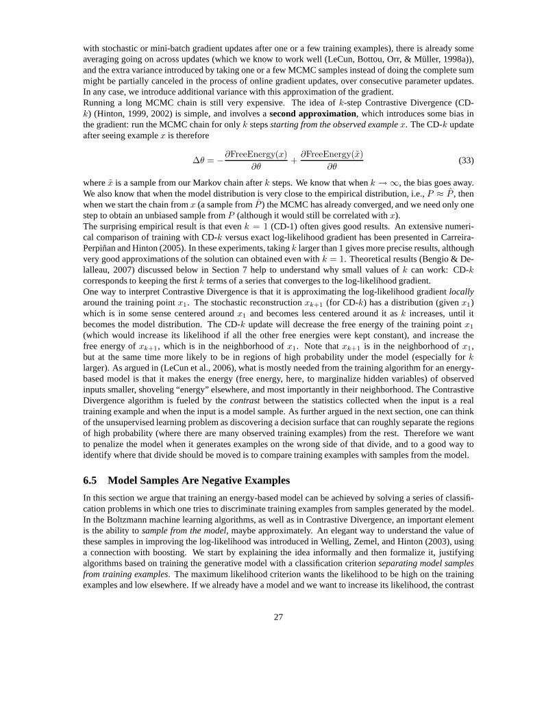
with stochastic or mini-batch gradient updates after one ora few training examples), there is already someaveraging going on across updates (which we know to work well(LeCun, Bottou, Orr, & Muller, 1998a)),and the extra variance introduced by taking one or a few MCMC samples instead of doing the complete summight be partially canceled in the process of online gradient updates, over consecutive parameter updates.In any case, we introduce additional variance with this approximation of the gradient.Running a long MCMC chain is still very expensive. The idea ofk-step Contrastive Divergence (CD-k) (Hinton, 1999, 2002) is simple, and involves asecond approximation, which introduces some bias inthe gradient: run the MCMC chain for onlyk stepsstarting from the observed examplex. The CD-k updateafter seeing examplex is therefore

∆θ = −∂FreeEnergy(x)

∂θ+

∂FreeEnergy(x)

∂θ(33)

wherex is a sample from our Markov chain afterk steps. We know that whenk → ∞, the bias goes away.We also know that when the model distribution is very close tothe empirical distribution, i.e.,P ≈ P , thenwhen we start the chain fromx (a sample fromP ) the MCMC has already converged, and we need only onestep to obtain an unbiased sample fromP (although it would still be correlated withx).The surprising empirical result is that evenk = 1 (CD-1) often gives good results. An extensive numeri-cal comparison of training with CD-k versus exact log-likelihood gradient has been presented inCarreira-Perpinan and Hinton (2005). In these experiments, takingk larger than 1 gives more precise results, althoughvery good approximations of the solution can obtained even with k = 1. Theoretical results (Bengio & De-lalleau, 2007) discussed below in Section 7 help to understand why small values ofk can work: CD-kcorresponds to keeping the firstk terms of a series that converges to the log-likelihood gradient.One way to interpret Contrastive Divergence is that it is approximating the log-likelihood gradientlocallyaround the training pointx1. The stochastic reconstructionxk+1 (for CD-k) has a distribution (givenx1)which is in some sense centered aroundx1 and becomes less centered around it ask increases, until itbecomes the model distribution. The CD-k update will decrease the free energy of the training pointx1

(which would increase its likelihood if all the other free energies were kept constant), and increase thefree energy ofxk+1, which is in the neighborhood ofx1. Note thatxk+1 is in the neighborhood ofx1,but at the same time more likely to be in regions of high probability under the model (especially forklarger). As argued in (LeCun et al., 2006), what is mostly needed from the training algorithm for an energy-based model is that it makes the energy (free energy, here, tomarginalize hidden variables) of observedinputs smaller, shoveling “energy” elsewhere, and most importantly in their neighborhood. The ContrastiveDivergence algorithm is fueled by thecontrastbetween the statistics collected when the input is a realtraining example and when the input is a model sample. As further argued in the next section, one can thinkof the unsupervised learning problem as discovering a decision surface that can roughly separate the regionsof high probability (where there are many observed trainingexamples) from the rest. Therefore we wantto penalize the model when it generates examples on the wrongside of that divide, and to a good way toidentify where that divide should be moved is to compare training examples with samples from the model.

6.5 Model Samples Are Negative Examples

In this section we argue that training an energy-based modelcan be achieved by solving a series of classifi-cation problems in which one tries to discriminate trainingexamples from samples generated by the model.In the Boltzmann machine learning algorithms, as well as in Contrastive Divergence, an important elementis the ability tosample from the model, maybe approximately. An elegant way to understand the value ofthese samples in improving the log-likelihood was introduced in Welling, Zemel, and Hinton (2003), usinga connection with boosting. We start by explaining the idea informally and then formalize it, justifyingalgorithms based on training the generative model with a classification criterionseparating model samplesfrom training examples. The maximum likelihood criterion wants the likelihood to be high on the trainingexamples and low elsewhere. If we already have a model and we want to increase its likelihood, the contrast

27

between where the model puts high probability (representedby samples) and where are the training exam-ples indicates how to change the model. If we were able to approximately separate training examples frommodel samples with a decision surface, we could increase likelihood by reducing the value of the energyfunction on one side of the decision surface (the side where there are more training examples) and increasingit on the other side (the side where there are more samples from the model). Mathematically, consider thegradient of the log-likelihood with respect to the parameters of theFreeEnergy(x) (or Energy(x) if wedo not introduce explicit hidden variables), given in eq. 16. Now consider a highly regularized two-classprobabilistic classifier which is only able to produce an output probabilityq(x) = P (y = 1|x) barely dif-ferent from 1

2 (hopefully on the right side more often than not). Letq(x) = sigm(a(x)), i.e., a(x) is thediscriminant function or an unnormalized conditional log-probability, just like the free energy. The averageconditional log-likelihood gradient for this probabilistic classifier is

EP

[∂ log P (y|x)

∂θ

]= EP

[∂(y log q(x) + (1− y) log(1− q(x)))

∂θ

]

= EP

[(1− q(x))

∂a(x)

∂θ

∣∣∣∣ y = 1

]− EP

[q(x)

∂a(x)

∂θ

∣∣∣∣ y = 0

]

≈1

2EP

[∂a(x)

∂θ

∣∣∣∣ y = 1

]−

1

2EP

[∂a(x)

∂θ

∣∣∣∣ y = 0

](34)

where the last equality is when the classifier is highly regularized: when the output weights are small,a(x)is close to 0 andq(x) ≈ 1

2 , so that(1 − q(x)) ≈ q(x). This expression for the log-likelihood gradientcorresponds exactly to the one obtained for energy-based models where the likelihood is expressed in termsof a free energy (eq. 16), when we interpret training examples as positive examples (y = 1) and modelsamples as negative examples (y = 0). One way to interpret this result is that if we could improveaclassifier that separated training samples from model samples, we could improve the log-likelihood of themodel, by putting more probability mass on the side of training samples. Practically, this could be achievedwith a classifier whose discriminant function was defined as the free energy of a generative model (up toa multiplicative factor), and assuming one could obtain samples (possibly approximate) from the model.A particular variant of this idea has been used to justify a boosting-like incremental algorithm for addingexperts in products of experts (Welling et al., 2003).

6.6 Variants of RBMs

We have already mentioned that it is straightforward to generalize the conditional distributions associatedwith visible or hidden units, e.g., to any member of the exponential family (Welling et al., 2003). Gaussianunits and exponential or truncated exponential units have been proposed or used in Freund and Haussler(1994), Welling et al. (2003), Bengio et al. (2007), Larochelle et al. (2007). With respect to the analysispresented here, the equations can be easily adapted by simply changing the domain of the sum (or integral)for thehi andxi. Diagonal quadratic terms (e.g., to yield Gaussian or truncated Gaussian distributions) canalso be added in the energy function without losing the property that the free energy factorizes.We review some of the more structural variations that have been proposed on the basic RBM model, in orderto increase its expressive power or exploit particular structure in the data.

6.6.1 Lateral Connections

The RBM can be made slightly less restricted by introducing interaction terms or “lateral connections” be-tween visible units. Samplingh fromP (h|x) is still easy but samplingx fromP (x|h) is now generally moredifficult, and amounts to sampling from a Markov Random Fieldwhich is also a fully observed Boltzmannmachine, in which the biases are dependent on the value ofh. Osindero and Hinton (2008) propose sucha model for capturing image statistics and their results suggest that Deep Belief Nets (DBNs) using suchmodules generate more realistic image patches than DBNs using ordinary RBMs. Their results also show

28

that the resulting distribution has marginal and pairwise statistics for pixel intensities that are similar to thoseobserved on real image patches.These lateral connections capture pairwise dependencies that can be more easily captured this way than usinghidden units, saving the work of hidden units for higher-order dependencies. In the case of the first layer, itcan be seen that this amounts to a form of whitening, which hasbeen found useful as a preprocessing step inimage processing systems (Olshausen & Field, 1997). The idea proposed in Osindero and Hinton (2008) isto use lateral connections at all levels of a DBN (which can now be seen as a hierarchy of Markov randomfields). The generic advantage of this type of approach wouldbe that the higher level factors represented bythe hidden units do not have to encode all the local “details”that the lateral connections at the levels belowcan capture. For example, when generating an image of a face,the approximate locations of the mouth andnose might be specified at a high level whereas their precise location could be selected in order to satisfythe pairwise preferences encoded in the lateral connections at a lower level. This appears to yield generatedimages with sharper edges and generally more accuracy in therelative locations of parts, without having toexpand a large number of higher-level units.In order to sample fromP (x|h), we can start a Markov chain at the current example (which presumablyalready has pixel co-dependencies similar to those represented by the model, so that convergence shouldbe quick) and only run a short chain. To reduce sampling variance in CD for this model, Osindero andHinton (2008) used five damped mean-field steps instead of an ordinary Gibbs chain on thex’s: xt =αxt−1 + (1− α)sigm(b + Uxt−1 + W ′h), with α ∈ (0, 1).

6.6.2 Conditional RBMs and Temporal RBMs

A Conditional RBM is an RBM where some of the parameters are not free but are instead parametrizedfunctions of another random variable. For example, consider an RBM for the joint distributionP (X, H)between observed vectorX and hidden vectorH , with parameters(b, c, W ) as per eq. 21, respectively forinput biasesb, hidden biasesc, and the weight matrixW . This idea has been introduced in Taylor, Hinton,and Roweis (2006) for context-dependent RBMs in which the hidden biasesc are affine functions of acontext variableC. Hence the RBM representsP (X, H |C), or marginalizing overH , P (X |C). In generalthe parametersθ of the RBM can be written as a parametrized functionθ = f(C; ω) with parametersω.The Contrastive Divergence algorithm for RBMs can be easilygeneralized to the case of Conditional RBMs.The CD gradient estimator∆θ on a parameterθ can be simply back-propagated to obtain a gradient estimatoronω:

∆ω = ∆θ∂θ

∂ω. (35)

In the affine caseb = β + MC (with b, β andC column vectors andM a matrix) studied in Taylor et al.(2006), the CD update on the conditional parameters is simply

∆β = ∆b

∆M = ∆b C′ (36)

where the last multiplication is an outer product, and∆b is the update given by CD-k.This idea has been successfully applied to model conditional distributionsP (xt|xt−1, xt−2, xt−3) in se-quential data of human motion (Taylor et al., 2006), wherext is a vector of joint angles and other geometricfeatures computed from motion capture data of human movements such as walking and running. Interest-ingly, this allowsgeneratingrealistic human motionsequences, by successively sampling thet-th framegiven the previously sampledk frames, i.e. approximating

P (x1, x2, . . . , xT ) ≈ P (x1, . . . xk)

T∏

t=k+1

P (xt|xt−1, . . . xt−k). (37)

The initial frames can be generated by using special null values as context or using a separate model forP (x1, . . . xk).

29

xtxt−1xt−2

htht−1ht−2

Figure 8: Example of Temporal RBM for modeling sequential data, including dependencies between thehidden variables. The double-arrow arc indicates an undirected connection, i.e. an RBM. The single-arrowarcs indicate conditional dependency: the(xt, ht) RBM is conditionned by the values of the past inputs andpast hidden vectors.

As demonstrated in Memisevic and Hinton (2007), it can be useful to make not just the biases but also theweights conditional on a context variable. In that case we greatly increase the number of degrees of freedom,introducing the capability to model three-way interactions between an input unitxi, a hidden unithj, and acontext unitck through interaction parametersUijk. This approach has been used withX an image andCthe previous image in a video, and the model learns to captureflow fields(Memisevic & Hinton, 2007).Probabilistic models of sequential data with hidden variablesHt (calledstate) can gain a lot by capturing thetemporal dependencies between the hidden variable at different timest in the sequence. This is what allowsHidden Markov Models (HMMs) (Rabiner & Juang, 1986) to capture dependencies in a long sequenceeven if the model only considers the hidden variable to be a Markov chain of order 1 (where the directdependence is only betweenHt andHt+1). Whereas the hidden variable representationHt in HMMs is local(all the possible values ofHt are enumerated and specific parameters associated with eachof these values),Temporal RBMs have been proposed (Sutskever & Hinton, 2007) to construct adistributed representation ofthe state. The idea is an extension of the Conditional RBM presented above, but where the context includesnot only past inputs but also past values of the state, e.g., we build a model of

P (Ht, Xt|Ht−1, Xt−1, . . . , Ht−k, Xt−k) (38)

where the context isCt = (Ht−1, Xt−1, . . . , Ht−k, Xt−k), as illustrated in Figure 8. Although samplingof sequences generated by Temporal RBMs can be done as in Conditional RBMs (with the same MCMCapproximation used to sample from RBMs, at each time step), exact inference of the hidden state sequencegiven an input sequence is not anymore tractable. Instead, Sutskever and Hinton (2007) propose to use amean-field filtering approximation of the hidden sequence posterior.

6.6.3 Factored RBMs

In several probabilistic language models, it has been proposed to learn a distributed representation of eachword (Deerwester, Dumais, Furnas, Landauer, & Harshman, 1990; Miikkulainen & Dyer, 1991; Bengioet al., 2001, 2003). For an RBM that models a sequence of words, it would be convenient to have aparametrization that automatically learns a distributed representation for each word in the vocabulary. Thisis essentially what Mnih and Hinton (2007) propose. They usea factorization of the weight matrixW intotwo factors, one that depends on the location in the input subsequence, and one that does not. Consider thecomputation of the hidden units’ probabilities given the input subsequence(w1, w2, . . . , wk), where eachword wt is represented by a one-hot vectorvt (all 0’s except for a 1 at positionwt) and these vectors areconcatenated into the input vectorx = (v1, . . . , vk). Instead of applying directly a matrixW to x, do the fol-lowing. First, each word symbolwt is mapped through a matrixR to ad-dimensional vectorR.,wt

= Rvt,

30

for t ∈ {1 . . . k}; second, the concatenated vectors(R.,w1, R.,w2

, . . . , R.,wk) = (Rv1, . . . Rvk) are multi-

plied by a matrixB. HenceW = B(R R . . .R), where(R R . . . R) indicates concatenation (not product)of R. This model has produced better out-of-sample log-likelihood than state-of-the-art language modelsbased on n-grams (Mnih & Hinton, 2007). This factorization can be combined with the temporal RBM ideaintroduced above, yielding further improvements in generalization performance (Mnih & Hinton, 2007).

7 Truncations of the Log-Likelihood in Gibbs-Chain Models

Here we approach the Contrastive Divergence update rule from a different perspective, which gives rise topossible generalizations of it and links it to the reconstruction error often used to monitor its performanceand that is used to optimize autoassociators (eq. 5). The inspiration for this derivation comes from Hintonet al. (2006): first from the idea (explained in Section 11.1)that the Gibbs chain can be associated with aninfinite directed graphical model (which here we associate to an expansion of the log-likelihood and of itsgradient), and second that the convergence of the chain justifies Contrastive Divergence (since the expectedvalue of eq. 33 becomes equivalent to eq. 15 when the chain sample x comes from the model).Consider a converging Markov chainxt ⇒ ht ⇒ xt+1 ⇒ . . . defined by conditional distributionsP (ht|xt)andP (xt+1|ht). A sufficient condition for convergence is that it mixes, i.e., one can reach any state fromany state in finite time.The following Lemma, demonstrated in (Bengio & Delalleau, 2007), shows that the by consecutive appli-cation of Bayes rule, one can expand the log-likelihood in a series that involves the samples in the Gibbschain.

Lemma 7.1. Consider the Gibbs chainx1 ⇒ h1 ⇒ x2 ⇒ h2 . . . starting at data pointx1. The log-likelihood can be expanded as follows for any path of the chain:

log P (x1) = log P (xt) +

t−1∑

s=1

logP (xs|hs)

P (hs|xs)+ log

P (hs|xs+1)

P (xs+1|hs)(39)

and consequently, since this is true for any path:

log P (x1) = E[log P (xt)] +

t−1∑

s=1

E

[log

P (xs|hs)

P (hs|xs)+ log

P (hs|xs+1)

P (xs+1|hs)

](40)

where the expectation is over the Markov chain, conditionalonx1.

In the limit t → ∞, the last term is just the entropy of distributionP (x). Note that the terms do not vanishast→∞, so as such this expansion does not justify truncating the series to approximate the log-likelihood.We will see that reconstruction error, often used for monitoring training progress of RBMs, is closely relatedto the first term in the series.Now consider the corresponding gradient series. To prove the theorem, the following simple lemma, whichwe use later, is very useful:

Lemma 7.2. For any modelP (Y ) with parametersθ,

E

[∂ log P (Y )

∂θ

]= 0 (41)

when the expected value is taken according toP (Y ).

31

Proof. We start from the sum to 1 constraint onP (Y ), differentiate and obtain the Lemma. To obtain thelast line below we use the fact that for any functionf(θ), we have∂f(θ)

∂θ = f(θ)∂ log f(θ)∂θ .

E[1] =∑

y

P (Y = y) = 1

∂∑

y P (Y = y)

∂θ=

∂1

∂θ= 0

∑

y

P (Y = y)∂ log P (Y = y)

∂θ= 0

The following theorem can then be proved (Bengio & Delalleau, 2007).

Theorem 7.3. Consider the converging Gibbs chainx1 ⇒ h1 ⇒ x2 ⇒ h2 . . . starting at data pointx1.The log-likelihood gradient can be expanded in a convergingseries as follows, where all expectations areconditional onx1:

∂ log P (x1)

∂θ=

t−1∑

s=1

(E

[∂ log P (xs|hs)

∂θ

]+ E

[∂ log P (hs|xs+1)

∂θ

])

+ E

[∂ log P (xt)

∂θ

](42)

with the terms ins converging to 0 ass→∞, and the final term (int) also converges to 0, ast→∞.

Since thek-th term becomes small ask increases, that justifies truncating the chain tok steps. Note howthe sums in the above expansion can be readily replaced by easy to obtain samples (for the firstk stepsin the Gibbs chain). This gives rise to a stochastic gradient, whose expected value is the exact expressionassociated with a truncation of the above log-likelihood gradient expansion. Finally, it can be shown (Bengio& Delalleau, 2007) that truncating to the firstk steps gives a parameter update that is exactly the CD-k updatein the case of a binomial RBM.

Corollary 7.4. When considering only the terms arising of the firstk steps in the Gibbs chainx1 ⇒ h1 ⇒x2 ⇒ h2 ⇒ . . . xk ⇒ hk, the unbiased stochastic estimator of the gradient of the truncated log-likelihoodexpansion of theorem 7.3 (with expectations replaced by samples in the chain) equals the CD-k update inthe case of a binomial RBM.

Experiments and theory support the idea that CD-k yields better and faster convergence (in terms of numberof iterations) than CD-(k−1) (but the computational overhead might not always be worth it). This is becausesmallerk corresponds to more bias in the estimation of the log-likelihood gradient. So CD-1 correspondsto taking the first two terms in the expansion (one sample ofh1|x1 and one sample ofx2|h1). What abouttaking only the first one? The first term in the log-likelihoodgradient expansion is

∑

h1

P (h1|x1)∂ log P (x1|h1)

∂θ(43)

Now consider a mean-field approximation of the above, in which instead of the average over allh1 configu-rations according toP (h1|x1) one replacesh1 by its average configurationh1 = E[h1|x1], yielding:

∂ log P (x1|h1)

∂θ(44)

32

which is minus the gradient ofreconstruction error ,

− logP (x1|h1) (45)

typically used to train autoassociators.So we have found that the truncation of the log-likelihood expansion gives rise to first approximation (1 term)to roughly reconstruction error (through a biased mean-field approximation), with slightly better approxi-mation (2 terms) to CD-1 (approximating the expectation by asample), and with more terms to CD-k. Notethat reconstruction error is deterministically computed and for this reason has been used to track progresswhen training RBMs with CD. Since reconstruction error and CD-k are complementary in terms of bias andvariance (as estimators of the log-likelihood gradient), it might be interesting to explore combinations ofthem: a low-variance high-bias estimator (reconstructionerror gradient) might be more useful at the begin-ning of training (where having a precise estimation of the gradient is less important) whereas the low-biashigh-variance estimator (CD-k) would be more useful to achieve training convergence.

8 Generalizing RBMs and Contrastive Divergence

Let us try to generalize the definition of RBM so as to include alarge class of parametrizations for whichessentially the same ideas and learning algorithms (Contrastive Divergence) that we have discussed abovecan be applied in a straightforward way. We generalize RBMs as follows: aGeneralized RBM is an energy-based probabilistic model with input vectorx and hidden vectorh whose energy function is such thatP (h|x)andP (x|h) both factorize. This definition can be formalized in terms ofthe parametrization of the energyfunction:

Proposition 8.1. The energy function associated with a model of the form of eq.11 such thatP (h|x) =∏i P (hi|x) andP (x|h) =

∏j P (xj |h) must have the form

Energy(x, h) =∑

j

φj(xj) +∑

i

ξi(hi) +∑

i,j

ηi,j(hi, xj). (46)

Proof. To achieve factorization ofP (h|x) we have already shown that the energy function must be writableas a sum overi (with one term perhi), in eq. 18. This gives us the constraint thatEnergy(x, h) can be writtenasEnergy(x, h) = −β(x) +

∑i γi(x, hi), for someβ andγi. Using the same arguments but inverting the

roles ofx andh, we obtain that the constraintEnergy(x, h) = −α(h) +∑

j ρj(xj , h) for someα andρj .Clearly if Energy(x, h) can be written as in eq. 46, then these two constraints are satisfied. On the otherhand, consider adding a term of a different from (not depending only onhi, only onxj , or only on a pair(hi, xj) to the right hand side of eq. 46. Then one of the above two constraints would be violated. Thereforethe above equation is the most general formulation that satisfies both factorization assumptions.

In the case where the hidden and input values are binary, thisnew formulation does not actually bringany additional power of representation. Indeed,ηi,j(hi, xj), which can take at most four different valuesaccording to the2× 2 configurations of(hi, xj ) could always be rewritten as a second order polynomial in(hi, xj): a + bhi + cxj + dhixj . However,b andc can be folded into the bias terms anda into a globaladdititive constant which does not matter (because it gets cancelled by the partition function).On the other hand, whenx or h are real-valued, one could imagine higher-capacity modeling of the(hi, xj)interaction, possibly non-parametric, e.g., gradually adding terms toηi,j so as to better model the interaction.Furthermore, sampling from the conditional densitiesP (xj |h) or P (hi|x) would be tractable even if theηi,j

are complicated functions, simply because these are 1-dimensional densities from which efficient approxi-mate sampling and numerical integration are easy (e.g., by computing cumulative sums of the density overnested subintervals or bins).This analysis also highlights the basic limitation of RBMs,which is that its parametrization only considerspairwise interactions between variables. It is because theh are hidden and that we can have as many hidden

33

units as we want that we still have full expressive power overpossible marginal distributions inx. Othervariants of RBMs discussed in Section 6.6 allow to introducethree-way interactions (Memisevic & Hinton,2007).Can Contrastive Divergence be applied to this generalized RBM formulation? Clearly, theorem 7.3 can stillbe applied. Furthermore, it can be shown, generalizing corollary 7.4 that considering only the firstk stepsof the Gibbs chain in the log-likelihood gradient expansion, one obtains an update rule similar to CD-k forbinomial RBMs.

Proposition 8.2. Consider a generalized RBM, with the energy function as in eq. 46. When consideringonly the terms arising of the firstk steps in the Gibbs chainx1 ⇒ h1 ⇒ x2 ⇒ h2 ⇒ . . . xk ⇒ hk, with theunbiased stochastic estimator of the gradient of the truncated log-likelihood expansion of theorem 7.3, allthe intermediate gradient terms cancel each other and the gradient estimator only depends directly on thefirst pair (x1, h1) and on the last pair(xk, hk), e.g., forθ a parameter ofηi,j :

t−1∑

s=1

E

[∂ log P (xs|hs)

∂θ+

∂ log P (hs|xs+1)

∂θ

]= E

∑

i,j

∂ηi,j(h1,i, x1,j)

∂θ−∑

i,j

∂ηi,j(hk,i, xk,j)

∂θ

(47)

wherehk,i is the i-th element of thek-th hidden vectorhk in the chain, and similarly forxk,j , and theexpectation is over the Markov chain, conditionned onx1.

Proof. Note that theφj andξi terms can be represented by extraηi,j terms so we will ignore them in theproof. By definition of our energy function and using the factorization of the conditionals shown above, wehave

P (hs,i|xs) =exp(

∑j ηi,j(hs,i, xs,j))

exp(∑

hs,i

∑j ηi,j(hs,i, xs,j))

(48)

and

P (xs+1,j |hs) =exp(

∑i ηi,j(hs,i, xs+1,j))

exp(∑

xs+1,j

∑i ηi,j(hs,i, xs+1,j))

(49)

Differentiating them and taking expectations with respectto the Markov chain, we find that the gradient of thedenominator oflog P (xs|hs) cancels the gradient of the numerator oflog P (hs|xs+1), and similarly that thegradient of the denominator oflog P (hs|xs+1) cancels the gradient of the numerator oflog P (xs+1|hs+1).

Hence, ignoring the remainderE[

∂ log P (xk+1)∂θ

]due to truncation of the series, there only remains from

eq. 42 the gradient of the numerator oflog P (x1|h1) and the gradient of the denominator oflog P (hk|xk+1).

Therefore, when generalizing RBMs with an energy function of the form of eq. 46, a Gibbs chain can stillbe run easily (thanks to Proposition 8.1), either to sample data from the model or for learning, and a CD-kalgorithm can be run to gradually tune the parameters, with the parameter update given by

∆θ =∑

i,j

∂ηi,j(h1,i, x1,j)

∂θ−∑

i,j

∂ηi,j(hk,i, xk,j)

∂θ(50)

with ε a learning rate for the stochastic gradient descent. Note that in most parametrizations we would havea particular element ofθ only depend on a particularηi,j (and no sum is needed). We recover Algorithm 1whenηi,j(h1,i, x1,j) = Wijh1,ix1,j and the other variants described in (Welling et al., 2005; Bengio et al.,2007) for different forms of the energy and allowed set of values for hidden and input units.

34

9 Stacked Autoassociators

Autoassociators have been used as building blocks to build adeep multi-layer neural network (Bengio et al.,2007; Ranzato et al., 2007; Larochelle et al., 2007). The training procedure is simpler than with Deep BeliefNetworks, so we start with it, noting that many variations onthat scheme are possible:

1. Train the first layer as an autoassociator to minimize someform of reconstruction error of the rawinput. This is purely unsupervised.

2. The hidden units’ outputs in the autoassociator are now used as input for another layer, also trained tobe an autoassociator. Again, we only need unlabeled examples.

3. Iterate as in (2) to add the desired number of layers.

4. Take the last hidden layer output as input to a supervised layer and initialize its parameters (eitherrandomly or by supervised training, keep the rest of the network fixed).

5. Fine-tune all the parameters of this deep architecture with respect to the supervised criterion. Alter-nately, unfold all the autoassociators into a very deep autoassociator and fine-tune the global recon-struction error, as in (Hinton & Salakhutdinov, 2006).

The hope is that the unsupervised initialization in a greedylayer-wise fashion has put the parameters of allthe layers in a region of parameter space from which a good local optimum can be reached by local descent.This indeed appears to happen in a number of tasks (Bengio et al., 2007; Ranzato et al., 2007; Larochelleet al., 2007).The principle is exactly the same as the one previously proposed for training Deep Belief Networks (Hintonet al., 2006), but using autoassociators instead of RBMs. Comparative experimental results in (Bengio et al.,2007; Larochelle et al., 2007) suggest that Deep Belief Networks typically (but not systematically) have aslight edge over stacked autoassociators, maybe because CD-k is closer to the log-likelihood gradient thanthe reconstruction error gradient. However, since the reconstruction error gradient has less variance thanCD-k (because no sampling is involved), it might be interesting to combine the two criteria, at least in theinitial phases of learning.An advantage of using autoassociators instead of RBMs as theunsupervised building block of a deep ar-chitecture is that almost any parametrizations of the layers are possible, as long as the training criterion iscontinuous in the parameters. On the other hand, the class ofprobabilistic models for which CD or otherknown tractable estimators of the log-likelihood gradientcan be applied is currently more limited. A dis-advantage of stacked autoassociators is that they do not correspond to a generative model: with generativemodels such as RBMs and DBNs, samples can be drawn to check qualitatively what has been learned, e.g.,by visualizing the images or word sequences that the model sees as plausible.Note that the above algorithm can be naturally in the semi-supervised setting, where only a fraction of thetraining examples are associated with a supervision label.For unlabeled examples only an unsupervisedcriterion is used (e.g., reconstruction error at each levelor over the whole network), whereas for supervisedexamples the supervised criterion is used. For labeled examples, both criteria can be combined. Combiningboth criteria has been found useful not only at the fine-tuning stage (where all the layers are jointly optimized)but also during the greedy layerwise stage (Bengio et al., 2007). This form ofpartial supervisionhas beenfound useful in cases where the true input distribution is not very informative of the target conditionaldistribution that one wants to capture for the supervised task.

35

10 Deep Belief Networks

A Deep Belief Network (Hinton et al., 2006) withlayers models the joint distribution between observedvectorx and` hidden layershk as follows:

P (x,h1, . . . ,h`) =

(`−2∏

k=1

P (hk|hk+1)

)P (h`−1,h`) (51)

wherex = h0, P (hk−1|hk) is a conditional distribution for visible hidden units in anRBM associated with

level k of the DBN, andP (h`−1,h`) is the visible-hidden joint distribution in the top-level RBM. This isillustrated in Figure 9.

Algorithm 2TrainUnsupervisedDBN(p, ε, L,n,W ,b)Train a DBN in a purely unsupervised way, with the greedy layer-wise procedure in which each added layeris trained as an RBM by contrastive divergence.p is the input training distribution for the networkε is a learning rate for the stochastic gradient descent in Contrastive DivergenceL is the number of layers to trainn = (n1, . . . , nL) is the number of hidden units in each layerW i is the weight matrix for leveli, for i from 1 toLbi is the bias vector for leveli, for i from 0 toL

• initialize b0 = 0for ` = 1 to L do• initialize W i = 0, bi = 0while not stopping criteriondo• sampleh0 = x from pfor k = 1 to `− 1 do• samplehk from Q(hk|hk−1)

end for• RBMupdate(h`−1, ε, W `, b`, b`−1) {thus providingQ(h`|h`−1) for future use}

end whileend for

When we train the DBN in a greedy layerwise fashion, as illustrated with the pseudo-code of Algorithm 2,each layer is initialized as an RBM, and we denoteQ(hk,hk−1) the k-th RBM trained in this way. Wewill use Q(hk|hk−1) as an approximation ofP (hk|hk−1), because it is easy to compute and sample fromQ(hk|hk−1) (which factorizes), and not fromP (hk|hk−1) (which does not). TheseQ(hk|hk−1) can also beused to construct a representation of the input vectorx. To obtain an approximate posterior or representationfor all the levels, we use the following procedure. First sampleh

1 ∼ Q(h1|x) from the first-level RBM, oralternatively with a mean-field approach useh

1 = E[h1|h0] instead of a sample ofh1, where the expectationis over the RBM distributionQ(hk|hk−1). This is just the output probabilities of the hidden units, in thecommon case where they are binomial units:h

1i = sigm(b1 + W 1

i x). Taking either the sampleh1 or themean-field vectorh1 as input for the second-level RBM, computeh2 or a sampleh2, etc. until the last layer.A sample of the DBN generative model forx can be obtained as follows:

1. Sample a visible vectorh`−1 from the top-level RBM. This can be achieved approximately by runninga Gibbs chain in that RBM alternating betweenh

` ∼ P (h`|h`−1) andh`−1 ∼ P (h`−1|h`), as outlinedin Section 6.3.1. By starting the chain from a representationh

`−1 obtained from a training set example(through theQ′s as above), fewer Gibbs steps might be required.

36

Figure 9: Deep Belief Network as a generative model (generative path, with bold arcs) and a means to extractmultiple levels of representation of the input (recognition path, with dashed arcs). The top two layersh

2 andh

3 form an RBM (for their joint distribution). The lower layersform a directed graphical model (sigmoidbelief neth2 ⇒ h

1 ⇒ x) and the prior for the penultimate layerh2 is provided by the top-level RBM.

2. Fork = `−1 down to 1, samplehk−1 givenhk according to the level-k hidden-to-visible conditional

distributionP (hk−1|hk).

3. x = h0 is the DBN sample.

The principle of greedy layer-wise unsupervised training of each layer on top of the previously trained onescan be applied with RBMs as the building blocks for each layer(Hinton et al., 2006; Hinton & Salakhutdinov,2006; Bengio et al., 2007; Salakhutdinov & Hinton, 2007).

1. Train the first layer as an RBM that models the raw inputx = h0 as its visible layer.

2. As outlined above, use that first layer to obtain a representation of the input data that will be used asdata for the second layer. Two common solutions are to take hidden layer samples ofh1|h0 or the realvaluesh1 = E(h1|h0)) for this representation.

3. Train the second layer as an RBM, taking the transformed data (h1|x or h1(x)) as training example(for the visible layer of that RBM).

4. Iterate (2 and 3) for the desired number of layers, each time propagating upward either samples ormean values.

5. Fine-tune all the parameters of this deep architecture with respect to a proxy for the DBN log-likelihood, or with respect to a supervised training criterion (after adding extra learning machineryto convert the learned representation into supervised predictions).

The remark made at the end of Section 9 about semi-supervisedand partially supervised training also appliesto DBNs. Combining labeled data and unlabeled data is simplewith DBNs, and the partially supervisedsetting has been found experimentally useful for some tasks(Bengio et al., 2007).

37

11 Stochastic Variational Bounds for Joint Optimization of DBNLayers

In this section we discuss mathematical underpinnings of training algorithms for DBNs. The log-likelihoodof a DBN can be lower bounded using Jensen’s inequality, and as we discuss below, this can justify thegreedy layer-wise training strategy introduced in (Hintonet al., 2006) and described in Section 10. Startingfrom eq. 51 for a DBN joint distribution, writingh for h

1 (the first level hidden vector) to lighten notation,and introducing an arbitrary conditional distributionQ(h|x) we have

log P (x) = log∑

h

P (x, h)

= log∑

h

Q(h|x)P (x, h)

Q(h|x)

≥∑

h

Q(h|x) logP (x, h)

Q(h|x)

=∑

h

Q(h|x) (log P (x, h)− log Q(h|x))

= HQ(h|x) +∑

h

Q(h|x) (log P (h) + log P (x|h)) . (52)

whereHQ(h|x) is the entropy of the distributionQ(h|x). To see what the inequality is missing out, we canuse another derivation, which is again true for anyQ(h|x) andP . First multiply by1 =

∑h Q(h|x), then

useP (x) = P (x,h)P (h|x) , and multiply by1 = Q(h|x)

Q(h|x) and expand the terms:

log P (x) = (∑

h

Q(h|x)) log P (x) =∑

h

Q(h|x) logP (x, h)

P (h|x)

=∑

h

Q(h|x) logP (x, h)

P (h|x)

Q(h|x)

Q(h|x)

= HQ(h|x) +∑

h

Q(h|x) log P (x, h) +∑

h

Q(h|x) logQ(h|x)

P (h|x)

= KL(Q(h|x)||P (h|x)) + HQ(h|x) +∑

h

Q(h|x) (log P (h) + log P (x|h)) . (53)

So the missing term in inequality 52 is the Kullback-Lieblerdivergence between the two conditional distri-butionsQ(h|x) andP (h|x). Whereas we have chosen to useP to denote probabilities under the DBN, let ususeQ to denote probabilities under an RBM (which we will call the first level RBM) , and in the equationschooseQ(h|x) to be the hidden-given-visible conditional distribution of that first level RBM. We define thatfirst level RBM such thatQ(x|h) = P (x|h). In generalP (h|x) 6= Q(h|x). This is because although themarginalP (h) on the first layer hidden vectorh1 = h is determined by the upper layers in the DBN, theRBM marginalQ(h) only depends on the parameters of the RBM.

11.1 Unfolding RBMs into Infinite Directed Belief Networks

Before using the above decomposition of the likelihood to justify the greedy training procedure for DBNs,we need to establish a connection betweenP (h1) in a DBN and the corresponding marginalQ(h1) givenby the first level RBM. The interesting observation is that there exists a DBN whoseh1 marginal equals thefirst RBM h

1 marginal, i.e.P (h1) = Q(h1), as long the dimension ofh2 equals the dimension ofh0 = x.

38

W’

W

W’_3

W_3

W’_3...

...

W’

W

W’_1

W_2

RBM

RBM

xt

ht−1

xt−1

ht−2

h2

h1

x

Figure 10: An RBM can be unfolded as an infinite directed belief network with tied weights (see text), left.The weight matrixW or its transpose are used depending on the parity of the layerindex. This sequenceof random variables corresponds to a Gibbs Markov chain to generatext (for t large). On the right, thetop-level RBM in a DBN can also be unfolded in the same way, showing that a DBN is an infinite directedgraphical model in whichsomeof the layers are tied (all except the bottom few ones).

To see this, consider a second RBM whose weight matrix is the transpose of the first level RBM (that is whywe need the matching dimensions). Hence, by symmetry of the roles of visible and hidden in an RBM jointdistribution (when transposing the weight matrix), the marginal distribution over the visible vector of thesecond RBM is equal to the marginal distributionQ(h1) of the hidden vector of the first RBM.Another interesting explanation is given in (Hinton et al.,2006): consider the infinite Gibbs sampling Markovchain starting att = −∞ and terminating att = 0, alternating betweenx andh

1 for the first RBM, withvisible vectors sampled on event and hidden vectors on oddt. This chain can be seen as an infinite directedbelief network with tied parameters (all even steps use weight matrix W ′ while all odd ones use weightmatrixW ). Alternatively, we can summarize any sub-chain fromt = −∞ to t = τ by an RBM with weightmatrix W or W ′ according to the parity ofτ , and obtain a DBN with1 − τ layers (not counting the inputlayer), as illustrated in Figure 10. This argument also shows that a 2-layer DBN in which the second levelhas weights equal to the transpose of the first level weights is equivalent to a single RBM.

11.2 Variational Justification of Greedy Layerwise Training

Here we discuss the argument made in Hinton et al. (2006) thatadding one RBM layer improves the like-lihood of a DBN. Let us suppose we have trained an RBM to modelx, which provides us with a modelQ(x) expressed through two conditionalsQ(h1|x) andQ(x|h1). Exploiting the argument in the previ-

39

ous subsection, let us now initialize an equivalent 2-layerDBN, i.e., generatingP (x) = Q(x), by takingP (x|h1) = Q(x|h1) andP (h1,h2) given by a second-level RBM whose weights are the transpose of thefirst-level RBM. Now let us come back to eq. 53 above, and the objective of improving the DBN likelihoodby changingP (h1), i.e., keepingP (x|h1) andQ(h1|x) fixed but allowing the second level RBM to change.Starting fromP (x|h1) = Q(x|h1), the KL term is zero and the entropy term in eq. 53 does not dependon the DBNP (h1), so small improvements to the term withP (h1) guarantee an increase inlog P (x). Weare also guaranteed that further improvements of theP (h1) term (i.e. further training of the second RBM)cannot bring the log-likelihood lower than it was before thesecond RBM was added. This is simply becauseof the positivity of the KL and entropy terms: further training of the second RBM increases a lower boundon the log-likelihood, as argued in Hinton et al. (2006). This justifies training the second RBM to maximizethe expectation over the training set of

∑h1 Q(h1|x) log P (h1).

The second-level RBM is thus trained to maximize∑

x,h1

P (x)Q(h1|x) log P (h1) (54)

with respect toP (h1). This is the maximum-likelihood criterion for a model that sees examplesh1 obtainedas marginal samples from the joint distributionP (x)Q(h1|x). If there was no constraint onP (h1), themaximizer of the above training criterion would be its “empirical” or target distribution

P ∗(h1) =∑

x

P (x)Q(h1|x). (55)

If we keep the first-level RBM fixed, then the second-level RBMcould therefore be trained as follows:samplex from the training set, then sampleh1 ∼ Q(h1|x), and consider thath as a training sample for thesecond-level RBM.The same argument can be made to justify adding a third layer,etc. We obtain the greedy layer-wise trainingprocedure outlined in Section 10. In practice the requirement that layer sizes alternate is not satisfied, andconsequently neither is it common practice to initialize the newly added RBM with the transpose of theweights at the previous layer (Hinton et al., 2006; Bengio etal., 2007), although it would be interesting toverify experimentally (in the case where the size constraint is imposed) whether the initialization with thetranspose of the previous layer helps to speed up training.Note that as we continue training the second RBM (and this includes adding extra layers), there is no guaran-tee thatlog P (x) (in average over the training set) will monotonically increase. As our lower bound continu-ous to increase, the actual log-likelihood could start decreasing. Let us examine more closely how this couldhappen. It would require the KL term to decrease as the secondRBM continues to be trained. However, thisis unlikely in general: as the DBN’sP (h1) deviates more and more from the first RBM’s marginalQ(h1) onh

1, it is likely that the posteriorsP (h1|x) (from the DBN) andQ(h1|x) (from the RBM) deviate more andmore (sinceP (h1|x) ∝ P (x|h1)P (h1)), making the KL term in eq. 53 increase. As the training likelihoodfor the second RBM increases,P (h1) moves smoothly fromQ(h1) towardsP ∗(h1). Consequently, it seemsvery plausible that continued training of the second RBM is going to increase the DBN’s likelihood (not justinitially) and by transitivity, adding more layers will also likely increase the DBN’s likelihood.Another argument to explain why the greedy procedure works is the following (Hinton, NIPS’2007 tutorial).The training distribution for the second RBM (samplesh

1 from P ∗(h1)) looks more like data generated byan RBM than the original training distributionP (x). This is becauseP ∗(h1) was obtained by applying onesub-step of an RBM Gibbs chain on examples fromP (x), and we know that applying many Gibbs stepswould yield data from that RBM.Unfortunately, when we train an RBM that will not be the top-level level of a DBN, we are not taking intoaccount the fact that more capacity will be added later to improve the prior on the hidden units. Le Roux andBengio (2008) have proposed considering alternatives to Contrastive Divergence for training RBMs destinedto initialize intermediate layers of a DBN. The idea is to consider thatP (h) will be modeled with a very highcapacity model (the higher levels of the DBN). In the limit case of infinite capacity, one can write down what

40

that optimalP (h) will be: it is simply the stochastic transformation of the empirical distribution through thestochastic mappingQ(h|x) of the first RBM (or previous RBMs). Plugging this back into the expressionfor log P (x), one finds that a good criterion for training the first RBM is the KL divergence between thedata distribution and the distribution of the stochastic reconstruction vectors after one step of the Gibbschain. Experiments (Le Roux & Bengio, 2008) confirm that thiscriterion yields better optimization of theDBN (initialized with this RBM). Unfortunately, this criterion is not tractable since it involves summingover all configurations of the hidden vectorh. Tractable approximations of it might be considered. Anotherinteresting alternative, explored in the next section, is to directly work on joint optimization of all the layersof a DBN.

11.3 Joint Unsupervised Training of All the Layers

We discuss here how one could train the whole DBN with respectto the unsupervised log-likelihood. Thelog-likelihood decomposition in eq. 53

log P (x) = KL(Q(h|x)||P (h|x)) + HQ(h|x) +∑

h

Q(h|x) (log P (h) + log P (x|h)) . (56)

can be used not only to justify the greedy training algorithm, but also to justify learning algorithms in whichall the layers of a DBN are simultaneously updated, maybe after a greedy layerwise initialization phase.The top level of the DBN would be trained as an RBM, i.e., choosing P (h) to maximize∑

h Q(h|x) log P (h), whereh is the penultimate layer of the DBN, and the top level RBM represents thejoint distribution between the penultimate and top layer ofthe DBN.Instead of keeping the lower levels fixed, if we want to improve them while taking into account the particularsof higher levels, we can return to eq. 53 and compute an estimate of the gradient of the log-likelihood withrespect toP (x|h) andQ(h|x). To simplify the exposition we only consider the case of a 2-level DBN, butthe same principle can be easily generalized to any number oflevels.The gradient of the entropy ofQ(h|x) is easy to estimate stochastically, using one or more samples ofh ∼ Q(h|x). Consider a parameterθ that influencesQ(h|x). Using first ∂y

∂x = y ∂ log y∂x , and Lemma 7.2 in

the second line,

∂HQ(h|x)

∂θ= −

∑

h

Q(h|x)∂ log Q(h|x)

∂θ−∑

h

Q(h|x) log Q(h|x)∂ log Q(h|x)

∂θ

= −∑

h

Q(h|x) log Q(h|x)∂ log Q(h|x)

∂θ. (57)

A stochastic gradient with respect to a parameterθ of the first level that influencesP (x|h) is also easy toobtain, using a similar derivation:

∂∑

h Q(h|x) log P (x|h)

∂θ=

∑

h

Q(h|x)∂ log P (h|x)

∂θ+∑

h

Q(h|x) log P (h|x)∂ log Q(h|x)

∂θ(58)

In both cases, we samplex from the training set andh ∼ Q(h|x) and use the gradientslog Q(h|x)∂ log Q(h|x)∂θ

and ∂ log P (h|x)∂θ + log P (h|x)∂ log Q(h|x)

∂θ . Note that these estimators could have high variance becauselog Q(h|x) and log P (h|x) could be arbitrarily large. In fact their variance might grow linearly with thedimension of the hidden vector.The gradient of the KL divergence is more problematic, because we do not have a simple expression forP (h|x). The KL term in eq. 53 could potentially be ignored since it ispositive and we would be optimizinga lower bound on the log-likelihood. Instead, an approximation has been used in thewake-sleep algo-rithm for sigmoid belief networks (Hinton et al., 1995). The idea is to minimize the other KL divergence,

41

KL(P (h|x)||Q(h|x)). Indeed if we sample from the DBN, we obtain an(h, x) tuple fromP (x, h) that canbe used as target forQ(h|x). Again using Lemma 7.2 and∂y

∂x = y ∂ log y∂x ,

∂KL(P (h|x)||Q(h|x))

∂θ=

∑

h

P (h|x)

(log

P (h|x)

Q(h|x)

∂ log P (h|x)

∂θ+

∂ log P (h|x)

∂θ−

∂ log Q(h|x)

∂θ

)

=∑

h

P (h|x)

(log

P (h|x)

Q(h|x)

∂ log P (h|x)

∂θ−

∂ log Q(h|x)

∂θ

). (59)

As before, we can obtain a stochastic estimator, but thelog P (h|x)Q(h|x)

∂ log P (h|x)∂θ term might have high variance.

In the wake-sleep algorithm (Hinton et al., 1995) and its contrastive version for DBNs (Hinton et al., 2006),the parameters ofQ(h|x) and the parameters ofP (x|h) are decoupled. In the context of a DBN, for all levelsexcept the top one, there is no reason to believe that the optimal “generative weights” (those used inP (x|h))have to be equal (transposed) to the “recognition weights” (those used inQ(h|x)). The wake-sleep algorithmprovides an update rule for both. We know that the true posterior P (h|x) does not necessarily factorize(cannot be written as

∏i P (hi|x)) whereasQ(h|x) does factorize. The algorithm proceeds in two phases: the

wake phase and the sleep phase. In thewake phase, we start from a training samplex and compute samplesfrom the approximate posteriors given by theQ(hk|hk−1)’s at each level (starting fromh0 = x). Thesesamples(h0,h1, . . .h`−1) provide fully observed training data for updating theP (hk−1|hk) generativedistributions, i.e, a stochastic step in the direction of the following gradient is performed

∑

h1,...,h`−1

Q(h`−1|h`−2) . . .Q(h1|x)`−1∏

k=1

∂ log P (hk−1|hk)

∂θ. (60)

An update of the top-level RBM is also performed in the wake phase, withh`−1 as observation for its visiblevector. In thesleep phase, we generate a full observation(h0,h1,h`−1) from the model: we first sampleh

`−1 from the top-level RBM, and then sample eachhk according toP (hk|hk+1). This is then used as

fully observed training data for the recognition conditionalsQ(hk|hk−1), by making a stochastic step in thedirection of the following gradient:

∑

h0,...,h`−1

P (h`−1)P (h`−2|h`−1) . . . P (h0|h1)

`−1∏

k=1

∂ log Q(hk|hk−1)

∂θ. (61)

With respect to the log-likelihood gradient decompositionthat we have been describing in this section,the approximations performed with the wake-sleep algorithm are thus the following: (a) approximate thegradient with respect toKL(Q(h|x)||P (h|x)) by the gradient with respect toKL(P (h|x)||Q(h|x)), and(b) approximate

∑

h

P (h|x) logP (h|x)

Q(h|x)

∂ log P (h|x)

∂θ−∑

h

Q(h|x) logP (h|x)

Q(h|x)

∂ log Q(h|x)

∂θ≈ 0 (62)

which might be reasonable as long asQ(h|x) is a good approximation ofP (h|x). Experiments suggest thatthe wake-sleep algorithm can be used (albeit slowly) to fine-tune a DBN and improve both the generativemodel and its ability to classify correctly (Hinton et al., 2006).

12 Global Optimization Strategies

Although deep architectures promise a more efficient representation of a distribution, and hence better gen-eralization, they appear to come at the price of a more difficult optimization problem, as discussed earlier

42

in Section 5. Here, we draw connections between existing work and approaches that could help to deal thisdifficult optimization problem, based on the principle ofcontinuation methods(Allgower & Georg, 1980).Although they provide no guarantee to obtain the global optimum, these methods have been particularlyuseful in computational chemistry to find approximate solutions of difficult optimization problems involvingthe configurations of molecules (Coleman & Wu, 1994; More & Wu, 1996; Wu, 1997). The basic idea isto first solve a smoothed version of the problem and graduallyconsider less smoothing, with the intuitionthat a smooth version of the problem reveals the global picture. On defines a single-parameter family of costfunctionsCλ(θ) such thatC0 can be optimized easily (maybe convex inθ), while C1 is the criterion that weactually wish to minimize. One first minimizesC0(θ) and then gradually increasesλ while keepingθ at alocal minimum ofCλ(θ). Typically C0 is a highly smoothed version ofC1, so thatθ gradually moves intothe basin of attraction of the dominant (if not global) minimum ofC1.

12.1 Greedy Layerwise Training of DBNs as a Continuation Method

The greedy layerwise training algorithm for DBNs describedin Section 10 can be viewed as an approximatecontinuation method, as follows. First of all recall (Section 11.1) that an RBM (and in particular the top-levelRBM of a DBN) can be unfolded into an infinite directed graphical model with tied parameters. At eachstep of the greedy layerwise procedure, we untie the parameters of the top-level RBM from the parametersof penultimate level. So one can view the layerwise procedure as follows. The model structure remains thesame, an infinite chain of sigmoidal belief layers, but we change the constraint on the parameters at eachstep of the layerwise procedure. Initially all the layers are tied. After training the first RBM (i.e. optimizingunder this constraint), we untie the first level parameters from the rest. After training the second RBM (i.e.optimizing under this slightly relaxed constraint), we untie the second level parameters from the rest, etc.Instead of a continuum of training criteria, we have a discrete sequence of (presumably) gradually moredifficult optimization problems. By making the process greedy we fix the parameters of the firstk levelsafter they have been trained and only optimize the(k + 1)-th, i.e. train an RBM.It would not be difficult to transform this layerwise approach into a continuation method by introducing acontinuous parameterγk at each stepd of adding a level to the DBN, such that whenγk = 0 the parametersof the(k+1)-th level (and above) are still tied to those of thek-th, whereas whenγk = 1, they are completelyfree of that constraint. But even in its current, discrete version, this analysis suggests an explanation for thegood performance of the layerwise training approach in terms of reaching better optima, as evidenced incomparative experiments against the traditional optimization techniques in which all the levels are trainedtogether (Bengio et al., 2007).

12.2 Controlling Temperature

Even optimizing the log-likelihood of a single RBM might be adifficult optimization problem. It turns outthat the use of stochastic gradient (such as the one obtainedfrom CD-k) and small initial weights is againclose to a continuation method, and could easily be turned into one. Consider the family of optimizationproblems corresponding to theregularization path(Hastie, Rosset, Tibshirani, & Zhu, 2004) for an RBM,e.g., with`1 or `2 regularization of the parameters, the family of training criteria parametrized byλ ∈ (0, 1]:

Cλ(θ) = −∑

i

log Pθ(xi)− ||θ||2 log λ. (63)

Whenλ → 0, we haveθ → 0, and it can be shown that the RBM log-likelihood becomes convex in θ.Whenλ → 1, there is no regularization (note that some intermediate value of λ might be better in terms ofgeneralization, if the training set is small). Note that controlling the magnitude of the biases and weights inan RBM is equivalent to controlling thetemperature in a Boltzmann machine (a scaling coefficient for theenergy function). High temperature corresponds to a highlystochastic system, and at the limit a factorialand uniform distribution over the input. Low temperature corresponds to a more deterministic system whereonly a small subset of possible configurations are plausible.

43

Interestingly, stochastic gradient descent starting fromsmall weights gradually allows the weights to increasein magnitude, approximately following the regularizationpath.Early stoppingis a well-known and efficientcapacity control technique based on monitoring performance on a validation set during training and keepingthe best parameters in terms of validation set error. The mathematical connection between early stoppingand`2 regularization (along with margin) has already been established (Collobert & Bengio, 2004). Thereis no guarantee that the local minimum associated with each value ofλ in eq. 63 is tracked by simply lettingthe weights follow the stochastic gradient path. It would not be difficult to slightly change the stochasticgradient algorithm to gradually increaseλ when the optimization is near enough a local minimum for thecurrent value ofλ. Note that the same technique might be extended for other difficult non-linear optimizationproblems found in machine learning, such as training a deep supervised neural network. We want to startfrom a globally optimal solution and gradually track local minima, starting from heavy regularization andmoving slowly to little or none.

12.3 Shaping: Training with a Curriculum

Humans need about two decades to be trained as fully functional adults of our society. That training is highlyorganized, based on an education system and a curriculum which introduces different concepts at differenttimes, exploiting previously learned concepts to ease the learning of new abstractions. The idea of traininga learning machine with a curriculum can be traced back at least to (Elman, 1993). The basic idea is tostart small, learn easier aspects of the task or easier sub-tasks, and then gradually increase the difficultylevel. From the point of view of building representations, advocated here, the idea is to learn representationsthat capture low-level abstractions first, and then exploitthem and compose them to learn slightly higher-level abstractions necessary to explain more complex structure in the data. By choosing which examples topresent and in which order to present them to the learning system, one canguidetraining and remarkablyincrease the speed at which learning can occur. This idea is routinely exploited inanimal trainingand iscalledshaping(Skinner, 1958; Peterson, 2004).Shaping and the use of a curriculum can also be seen as continuation methods. For this purpose, considerthe learning problem of modeling the data coming from a training distributionP . The idea is to reweightthe probability of sampling the examples from the distribution according to a given schedule, starting fromthe “easiest” examples and moving gradually towards examples illustrating more abstract concepts. At pointt in the schedule, we train from distributionPt, with P1 = P andP0 chosen to be easy to learn. Like inany continuation method, we move along the schedule when thelearner has reached a local minimum atthe current pointt in the schedule, i.e., when it has sufficiently mastered the previously presented examples(sampled fromPt). By making small changes int correspond to smooth changes in the probability ofsampling examples in the training distribution, we can construct a continuous path starting from an easylearning problem and ending in the desired training distribution.There is a connection between the shaping/curriculum idea and the greedy layer-wise idea. In both cases wewant to exploit the notion that a high level abstraction can more conveniently be learned once appropriatelower-level abstractions have been learned. In the case of the layer-wise approach, this is achieved bygradually adding more capacity in a way that builds upon previously learned concepts. In the case of thecurriculum, we control the training examples so as to make sure that the simpler concepts have actually beenlearned before showing many examples of the more advanced concepts. Showing complicated illustrationsof the more advanced concepts is likely to be generally a waste of time, as suggested by the difficulty forhumans to grasp a new idea if they do not first understand the concepts necessary to express that new ideacompactly.With the curriculum idea we introduce a teacher, in additionto the learner and the training distribution orenvironment. The teacher can use two sources of informationto decide on the schedule: (a) prior knowledgeabout a sequence of concepts that can more easily be learned when presented in that order, and (b) monitoringof the learner’s progress to decide when to move on to new material from the curriculum. The teacher hasto select a level of difficulty for new examples which is a compromise between “too easy” (the learner will

44

not need to change its model to account for these examples) and “too hard” (the learner cannot make anincremental change that can account for these examples so they will most likely be treated as outliers orspecial cases, i.e. not helping generalization).

13 Other Comments

13.1 Deep + Distributed does not include only Neural

Although much of this paper has focused on deep neural net architectures, the idea of exploring learningalgorithms for deep architectures should be explored beyond the neural net framework. For example, itwould be interesting to consider extensions of decision tree and boosting algorithms to multiple levels, ashinted at the end of Section 3.3.Kernel-learning algorithms suggest another path which should be explored, since a feature space that cap-tures the abstractions relevant to the distribution of interest would be just the right space in which to applythe kernel machinery. Research in this direction should consider ways in which the learned kernel wouldhave the ability to generalize non-locally, to avoid the curse of dimensionality issues raised in Section 3.1when trying to learn a highly-varying function.

13.2 Why Sparse Representations and Not Dimensionality Reduction

We argue here that if one is going to have fixed-size representations (as in the brain), then sparse rep-resentations are more efficient to allow for varying number of bits per example. According to learningtheory (Vapnik, 1995; Li & Vitanyi, 1997), to obtain good generalization it is enough that the total numberof bits needed to encode thewhole training setbe small, compared to the size of the training set. In manydomains of interest different examples have different information content. This is why for example an imagecompression algorithm normally uses a different number of bits for different images (even if they all havethe same dimensions).On the other hand, dimensionality reduction algorithms, whether linear such as PCA and ICA, or non-linearsuch as LLE and Isomap, map each example to the same low-dimensional space. In light of the aboveargument, it would be more efficient to map each example to a variable-length representation. To simplifythe argument, assume this representation is a binary vector. If we are required to map each example to afixed-length representation, a good solution would be to choose that representation to have enough degreesof freedom to represent the vast majority of the examples, while at the same allowing to compress that fixed-length bit vector to a smaller variable-size code for most ofthe examples. We now have two representations:the fixed-length one, which we might use as input to make predictions and make decisions, and a smaller,variable-size one, which can in principle be obtained from the fixed-length one through a compression step.For example, if the bits in our fixed-length representation vector have a high probability of being 0 (i.e. asparsity condition), then for most examples it is easy to compress the fixed-length vector (in average by theamount of sparsity).Another argument in favor of sparsity is that the fixed-length representation is going to be used as input forfurther processing, so that it should be easy to interpret. Ahighly compressed encoding is usually completelyentangled, so that no subset of bits in the code can really be interpreted unless all the other bits are taken intoaccount. Instead, we would like our fixed-length sparse representation to have the property that individualbits or small subsets of these bits can be interpreted, i.e.,correspond to meaningful aspects of the input, andcapture factors of variation in the data. For example, with aspeech signal as input, if some bits encode thespeaker characteristics and other bits encode generic features of the phoneme being pronounced, we havedisentangled some of the factors of variation in the data, and some subset of the factors might be sufficientfor some particular prediction tasks.Another way to justify sparsity of the representation was proposed in Ranzato et al. (2008). This view actu-ally explains how one could get good models even though the partition function is not explicitly maximized,

45

or only maximized approximately, as long as other constraints (such as sparsity) are used on the learned rep-resentation. Suppose that the representation learned by anautoassociator is sparse, then the autoassociatorcannot reconstruct well every possible input pattern. To minimize the average reconstruction error on thetraining set, the autoassociator then has to find a representation which captures statistical regularities of thedata distribution. First of all, Ranzato et al. (2008) connect the free energy with a form of reconstructionerror (when one replaces summing over hidden unit configurations by maximizing over them). Minimizingreconstruction error on the training set therefore amountsto minimizing free energy, i.e., maximizing thenumerator in eq. 13. Since the denominator (the partition function) is just a sum of the numerator over allpossible input configurations, we would like to make reconstruction error high for most input configurations.This can be achieved if the encoder (which maps an input to itsrepresentation) is constrained in such a waythat it cannot represent well most of the possible input patterns (i.e., the reconstruction error is high formost possible input patterns). One approach is to impose a sparsity penalty on the representation Ranzatoet al. (2008), which can be incorporated in the training criterion. In this way, the term of the log-likelihoodgradient associated with the partition function is completely avoided, and replaced by a sparsity penalty onthe hidden unit code. Interestingly, this idea could potentially be used to improve RBM training, which onlyuses anapproximateestimator of the gradient of the log of the partition function. If we add a penalty sparsityto the hidden representation, we may compensate for the weaknesses of that approximation, by making surewe increase the free energy of most possible input configuations, and not only of the reconstructed neighborsof the input example that are obtained in the negative phase of Contrastive Divergence.

13.3 Other Reasons Why Unsupervised Learning is Crucial

One of the claims of this paper is that powerful unsupervisedor semi-supervised learning is a crucial com-ponent in building successful learning algorithms for deeparchitectures aimed at AI. We briefly cover thearguments in favor of this hypothesis here:

• Unknown future tasks: if a learning agent does not know what future learning tasks it will have todeal with in the future, but it knows that the task will be defined with respect to a world (i.e. randomvariables) that it can observe now, it would appear very rational to collect as much information aspossible about this world so as to learn what makes it tick.

• Once a good high-level representation is learned, other learning tasks (e.g., supervised or reinforce-ment learning) could be much easier. We know for example thatkernel machines can be very powerfulif using an appropriate kernel, i.e. an appropriate featurespace. Similarly, we know powerful rein-forcement learning algorithms which have guarantees in thecase where the actions are essentiallyobtained through linear combination of appropriate features. We do not know what the appropriaterepresentation should be, but one would be reassured if it captured the salient factors of variation inthe input data, and disentangles them.

• Layer-wise unsupervised learning: this was argued in Section 5.3. Much of the learning could be doneusing information available locally in one layer or sub-layer of the architecture, thus avoiding thehypothesized problems with supervised gradients propagating through long chains with large fan-inelements.

• Connected to the two previous points is the idea that unsupervised learning could put the parametersof a supervised or reinforcement learning machine in a region from which gradient descent (local op-timization) would yield good solutions. This has been verified empirically in cases studied in Bengioet al. (2007).

• Less prone to overfitting: it has been argued (Hinton, 2006) that unsupervised learning is less proneto overfitting than supervised learning. The intuition is the following. When doing discriminantclassification, one only needs to learn a function whose variations matter near the decision boundary.

46

A very small subset of the input variations might be relevantto uncover the proper classification.On the other hand, unsupervised learning tries to capture all the variations in the input. Therefore itrequires a lot more capacity, or equivalently, is less proneto overfitting at equal capacity and equalnumber of training examples. Unsupervised learning can be used to initialize or regularize in thecontext of supervised learning systems.

• The extra constraints imposed on the optimization by requiring the model to capture not only the input-to-target dependency but also the statistical regularities of the input distribution might be helpful inavoiding some local minima (those that do not correspond to good modeling of the input distribution).

14 Open Questions

Research on deep architectures is still young and many questions remain unanswered. The following arepotentially interesting.

1. Can the results pertaining to the role of computational depth in circuits be generalized beyond logicgates and linear threshold units?

2. Is there a depth that is mostly sufficient for the computations necessary to achieve AI?

3. How can the theoretical results on depth of circuits with afixed size input be generalized to dynamicalcircuits operating in time, with context and the possibility of recursive computation?

4. Why is gradient-based training of deep neural networks from random initialization often unsuccessful?

5. Are RBMs trained by CD doing a good job of preserving the information in their input, and if not howcan that be fixed?

6. Is the presence of local minima an important issue in training RBMs?

7. Could we replace RBMs by algorithms that would be proficient at extracting good representations butinvolving an easier optimization problem, perhaps even a convex one?

8. Should the number of Gibbs steps in Contrastive Divergence be adjusted during training?

9. Besides reconstruction error, are there other more appropriate ways to monitor progress during trainingof RBMs? Equivalently, are there tractable approximationsof the partition function in RBMs?

10. Could RBMs and autoassociators be improved by imposing some form of sparsity penalty on therepresentations they learn, and what would be good ways to doso?

11. Without increasing the number of hidden units, can the capacity of an RBM be increased using non-parametric forms of its energy function?

12. Is there a probabilistic interpretation to models learned in stacked autoassociators?

13. How efficient is the greedy layer-wise algorithm for training Deep Belief Networks (in terms of max-imizing the training data likelihood)? Is it too greedy?

14. Can we obtain low variance and low bias estimators of the log-likelihood gradient in Deep BeliefNetworks, i.e., can we jointly train all the layers (with respect to the unsupervised objective)?

15. Can optimization strategies based on continuation methods deliver significantly improved training ofDeep Belief Networks?

16. Aren’t there other efficiently trainable deep architectures besides the Deep Belief Network model?

47

17. Is a curriculum needed to learn the kinds of high-level abstractions that humans take years or decadesto learn?

18. Can the principles discovered to train deep architectures be applied or generalized to train recurrentnetworks or dynamical belief networks, which learn to represent context and long-term dependencies?

19. Could we compute a tractable proxy for log-likelihood inDeep Belief Networks that could be used tomonitor their performance during training, even in the unsupervised case?

20. How can deep architectures be generalized to represent information that, by its nature, might seem noteasily representable by vectors, because of its variable size and structure (e.g. trees, graphs)?

21. Although Deep Belief Networks are in principle well suited for the semi-supervised setting, howshould their algorithms be adapted to this setting and how would they fare compared to existing semi-supervised algorithms?

22. When labeled examples are available, how should supervised and unsupervised criteria be combinedto learn the model’s representations of the input?

23. Can we find analogs of the computations necessary for Contrastive Divergence and Deep Belief Netlearning in the brain?

24. Can decision tree ensembles be stacked to obtain and train a different type of deep architecture?

15 Conclusion

This paper started with a number of motivations: first to use learning to approach AI, then on the intuitiveplausibility of decomposing a problem into multiple levelsof computation and representation, followedby theoretical results showing that a computational architecture that does not have enough of these levelscan require a huge number of computational elements, and a learning algorithm that relies only on localgeneralization is unlikely to generalize well when trying to learn highly-varying functions.Turning to architectures and algorithms, we first motivateddistributed representations of the data, in whicha huge number of possible configurations of abstract features of the input are possible, allowing a system tocompactly represent each example, while opening the door toa rich form of generalization. The discussionthen focused on the difficulty of optimizing deep architectures for learning multiple levels of distributedrepresentations. Although the reasons for the failure of standard gradient-based methods in this case remainto be clarified, several algorithms have been introduced in recent years that demonstrate much better perfor-mance than was previously possible with simple gradient-based optimization, and we have tried to focus onthe underlying principles behind their success.The paper focussed on a particular family of algorithms, theDeep Belief Networks, and their componentelements, the Restricted Boltzmann Machine. We studied andconnected together estimators of the log-likelihood gradient in Restricted Boltzmann machines, helping to justify the use of the Contrastive Diver-gence update for training Restricted Boltzmann Machines. We highlighted an optimization principle thathas worked well for Deep Belief Networks and related algorithms such as Stacked Autoassociators, basedon a greedy, layerwise, unsupervised initialization of each level of the model. We found that this optimiza-tion principle is actually an approximation of a more general optimization principle, exploited in so-calledcontinuation methods, in which a series of gradually more difficult optimization problems are solved. Thissuggested new avenues for optimizing deep architectures, either by tracking solutions along a regulariza-tion path, or by presenting the system with a sequence of selected examples illustrating gradually morecomplicated concepts, in a way analogous to the way studentsor animals are trained.

48

Acknowledgements

The author is particularly grateful for the inspiration from and constructive discussions with Yann Le Cun,Geoffrey Hinton, Joseph Turian, Aaron Courville, Hugo Larochelle, Olivier Delalleau, Nicolas Le Roux,Jerome Louradour, Pascal Lamblin, James Bergstra, and Dumitru Erhan. This research was performedthanks to funding from NSERC, MITACS, and the Canada Research Chairs.

References

Ackley, D., Hinton, G., & Sejnowski, T. (1985). A learning algorithm for Boltzmann machines.CognitiveScience, 9.

Allgower, E. L., & Georg, K. (1980).Numerical Continuation Methods. An Introduction. No. 13 in SpringerSeries in Computational Mathematics. Springer-Verlag.

Andrieu, C., de Freitas, N., Doucet, A., & Jordan, M. (2003).An introduction to MCMC for machinelearning.Machine Learning, 50, 5–43.

Baxter, J. (1995). Learning internal representations. InProceedings of the Eighth International Conferenceon Computational Learning Theory, pp. 311–320 Santa Cruz, California. ACM Press.

Baxter, J. (1997). A bayesian/information theoretic modelof learning via multiple task sampling.MachineLearning, 28, 7–40.

Belkin, M., & Niyogi, P. (2003). Using manifold structure for partially labeled classification. In Becker,S., Thrun, S., & Obermayer, K. (Eds.),Advances in Neural Information Processing Systems 15Cam-bridge, MA. MIT Press.

Belkin, M., Matveeva, I., & Niyogi, P. (2004). Regularization and semi-supervised learning on large graphs.In Shawe-Taylor, J., & Singer, Y. (Eds.),COLT’2004. Springer.

Bell, A., & Sejnowski, T. (1995). An information maximisation approach to blind separation and blinddeconvolution.Neural Computation, 7(6), 1129–1159.

Bengio, Y., Ducharme, R., & Vincent, P. (2001). A neural probabilistic language model. In Leen, T.,Dietterich, T., & Tresp, V. (Eds.),Advances in Neural Information Processing Systems 13, pp. 933–938. MIT Press.

Bengio, Y., Lamblin, P., Popovici, D., & Larochelle, H. (2007). Greedy layer-wise training of deep networks.In Scholkopf, B., Platt, J., & Hoffman, T. (Eds.),Advances in Neural Information Processing Systems19, pp. 153–160. MIT Press.

Bengio, Y., Simard, P., & Frasconi, P. (1994). Learning long-term dependencies with gradient descent isdifficult. IEEE Transactions on Neural Networks, 5(2), 157–166.

Bengio, Y., & Delalleau, O. (2007). Justifying and generalizing contrastive divergence. Tech. rep. 1311,Dept. IRO, Universite de Montreal.

Bengio, Y., Delalleau, O., & Le Roux, N. (2006). The curse of highly variable functions for local kernelmachines. In Weiss, Y., Scholkopf, B., & Platt, J. (Eds.),Advances in Neural Information ProcessingSystems 18, pp. 107–114. MIT Press, Cambridge, MA.

Bengio, Y., Delalleau, O., Le Roux, N., Paiement, J.-F., Vincent, P., & Ouimet, M. (2004). Learning eigen-functions links spectral embedding and kernel PCA.Neural Computation, 16(10), 2197–2219.

49

Bengio, Y., Delalleau, O., & Simard, C. (2007). Decision trees do not generalize to new variations. Tech.rep. 1304, Universite de Montreal, Dept. IRO.

Bengio, Y., Ducharme, R., Vincent, P., & Jauvin, C. (2003). Aneural probabilistic language model.Journalof Machine Learning Research, 3, 1137–1155.

Bengio, Y., & Le Cun, Y. (2007). Scaling learning algorithmstowards AI. In Bottou, L., Chapelle, O.,DeCoste, D., & Weston, J. (Eds.),Large Scale Kernel Machines. MIT Press.

Boser, B., Guyon, I., & Vapnik, V. (1992). A training algorithm for optimal margin classifiers. InFifthAnnual Workshop on Computational Learning Theory, pp. 144–152 Pittsburgh.

Bourlard, H., & Kamp, Y. (1988). Auto-association by multilayer perceptrons and singular value decompo-sition. Biological Cybernetics, 59, 291–294.

Brand, M. (2003). Charting a manifold. In Becker, S., Thrun,S., & Obermayer, K. (Eds.),Advances inNeural Information Processing Systems 15. MIT Press.

Breiman, L., Friedman, J. H., Olshen, R. A., & Stone, C. J. (1984). Classification and Regression Trees.Wadsworth International Group, Belmont, CA.

Breiman, L. (2001). Random forests.Machine Learning, 45(1), 5–32.

Carreira-Perpinan, M., & Hinton, G. (2005). On contrastive divergence learning. InProceedings of theTenth International Workshop on Artificial Intelligence and Statistics, Jan 6-8, 2005, Savannah Hotel,Barbados.

Caruana, R. (1993). Multitask connectionist learning. InProceedings of the 1993 Connectionist ModelsSummer School, pp. 372–379.

Cohn, D., Ghahramani, Z., & Jordan, M. I. (1995). Active learning with statistical models. In Tesauro, G.,Touretzky, D., & Leen, T. (Eds.),Advances in Neural Information Processing Systems 7. CambridgeMA: MIT Press.

Coleman, T. F., & Wu, Z. (1994). Parallel continuation-based global optimization for molecular conforma-tion and protein folding. Tech. rep., Cornell University, Department of Computer Science.

Collobert, R., & Bengio, S. (2004). Links between perceptrons, mlps and svms. InICML ’04: Twenty-firstinternational conference on Machine learningNew York, NY, USA. ACM Press.

Cortes, C., Haffner, P., & Mohri, M. (2004). Rational kernels: Theory and algorithms.Journal of MachineLearning Research, 5, 1035–1062.

Cortes, C., & Vapnik, V. (1995). Support vector networks.Machine Learning, 20, 273–297.

Cristianini, N., Shawe-Taylor, J., Elisseeff, A., & Kandola, J. (2002). On kernel-target alignment.Advancesin Neural Information Processing Systems, 14, 367–373.

Cucker, F., & Grigoriev, D. (1999). Complexity lower boundsfor approximation algebraic computationtrees.Journal of Complexity, 15(4), 499–512.

Dayan, P., Hinton, G., Neal, R., & Zemel, R. (1995). The Helmholtz machine. Neural Computation, 7,889–904.

Deerwester, S., Dumais, S., Furnas, G., Landauer, T., & Harshman, R. (1990). Indexing by latent semanticanalysis.Journal of the American Society for Information Science, 41(6), 391–407.

50

Delalleau, O., Bengio, Y., & Le Roux, N. (2005). Efficient non-parametric function induction in semi-supervised learning. In Cowell, R., & Ghahramani, Z. (Eds.), Proceedings of the Tenth InternationalWorkshop on Artificial Intelligence and Statistics, Jan 6-8, 2005, Savannah Hotel, Barbados, pp. 96–103. Society for Artificial Intelligence and Statistics.

Doi, E., Balcan, D. C., & Lewicki, M. S. (2006). A theoreticalanalysis of robust coding over noisy over-complete channels. In Weiss, Y., Scholkopf, B., & Platt, J.(Eds.),Advances in Neural InformationProcessing Systems 18, pp. 307–314. MIT Press, Cambridge, MA.

Elman, J. L. (1993). Learning and development in neural networks: The importance of starting small..Cognition, 48, 781–799.

Freund, Y., & Haussler, D. (1994). Unsupervised learning ofdistributions on binary vectors using two layernetworks. Tech. rep. UCSC-CRL-94-25, University of California, Santa Cruz.

Freund, Y., & Schapire, R. E. (1996). Experiments with a new boosting algorithm. InMachine Learning:Proceedings of Thirteenth International Conference, pp. 148–156 USA. ACM.

Fukushima, K. (1980). Neocognitron: A self-organizing neural network model for a mechanism of patternrecognition unaffected by shift in position.Biological Cybernetics, 36, 193–202.

Gartner, T. (2003). A survey of kernels for structured data. ACM SIGKDD Explorations Newsletter, 5(1).

Geman, S., & Geman, D. (1984). Stochastic relaxation, gibbsdistributions, and the bayesian restoration ofimages.IEEE Transactions on Pattern Analysis and Machine Intelligence, 6.

Hastad, J. (1986). Almost optimal lower bounds for small depth circuits. InProceedings of the 18th annualACM Symposium on Theory of Computing, pp. 6–20 Berkeley, California. ACM Press.

Hastad, J., & Goldmann, M. (1991). On the power of small-depth threshold circuits.Computational Com-plexity, 1, 113–129.

Hastie, T., Rosset, S., Tibshirani, R., & Zhu, J. (2004). Theentire regularization path for the support vectormachine.Journal of Machine Learning Research, 5, 1391–1415.

Hinton, G. E., Osindero, S., & Teh, Y. (2006). A fast learningalgorithm for deep belief nets.NeuralComputation, 18, 1527–1554.

Hinton, G. E., & Sejnowski, T. J. (1986). Learning and relearning in Boltzmann machines. In Rumelhart,D. E., & McClelland, J. L. (Eds.),Parallel Distributed Processing: Explorations in the Microstructureof Cognition. Volume 1: Foundations. MIT Press, Cambridge, MA.

Hinton, G. (1986). Learning distributed representations of concepts. InProceedings of the Eighth AnnualConference of the Cognitive Science Society, pp. 1–12 Amherst 1986. Lawrence Erlbaum, Hillsdale.

Hinton, G. (2002). Training products of experts by minimizing contrastive divergence.Neural Computation,14, 1771–1800.

Hinton, G. (2006). To recognize shapes, first learn to generate images. Tech. rep. UTML TR 2006-003,University of Toronto.

Hinton, G., Dayan, P., Frey, B., & Neal, R. (1995). The wake-sleep algorithm for unsupervised neuralnetworks.Science, 268, 1558–1161.

Hinton, G., Sejnowski, T., & Ackley, D. (1984). Boltzmann machines: Constraint satisfaction networks thatlearn. Tech. rep. TR-CMU-CS-84-119, Carnegie-Mellon University, Dept. of Computer Science.

51

Hinton, G., Welling, M., Teh, Y., & Osindero, S. (2001). A newview of ica. InProceedings of ICA-2001San Diego, CA.

Hinton, G. (1999). Products of experts. InProceedings of the Ninth International Conference on ArtificialNeural Networks (ICANN), Vol. 1, pp. 1–6.

Hinton, G. E., & Salakhutdinov, R. (2006). Reducing the Dimensionality of Data with Neural Networks.Science, 313, 504–507.

Hinton, G. E., & Zemel, R. S. (1994). Autoencoders, minimum description length, and Helmholtz freeenergy.Advances in Neural Information Processing Systems, 6, 3–10.

Ho, T. K. (1995). Random decision forest. In3rd International Conference on Document Analysis andRecognition, pp. 278–282 Montreal, Canada.

Hochreiter, S. (1991). Untersuchungen zu dynamischen neuronalen Netzen. Diploma thesis, Institut furInformatik, Lehrstuhl Prof. Brauer, Technische Universitat Munchen.. See www7.informatik.tu-muenchen.de/˜hochreit.

Hotelling, H. (1933). Analysis of a complex of statistical variables into principal components.Journal ofEducational Psychology, 24, 417–441, 498–520.

Hubel, D., & Wiesel, T. (1962). Receptive fields, binocular interaction, and functional architecture in thecat’s visual cortex.Journal of Physiology (London), 160, 106–154.

Hutter, M. (2005).Universal Artificial Intelligence: Sequential Decisions based on Algorithmic Probability.Springer, Berlin.

Intrator, N., & Edelman, S. (1996). How to make a low-dimensional representation suitable for diverse tasks.Connection Science, Special issue on Transfer in Neural Networks, 8, 205–224.

Jaakkola, T., & Haussler, D. (1998). Exploiting generativemodels in discriminative classifiers..

Japkowicz, N., Hanson, S. J., & Gluck, M. A. (2000). Nonlinear autoassociation is not equivalent to PCA.Neural Computation, 12(3), 531–545.

Kolmogorov, A. N. (1965). Three approaches to the quantitative definition of information. Problems ofInformation and Transmission, 1(1), 1–7.

Lanckriet, G., Cristianini, N., Bartlett, P., El Gahoui, L., & Jordan, M. (2002). Learning the kernel matrixwith semi-definite programming. InICML’2002.

Larochelle, H., Erhan, D., Courville, A., Bergstra, J., & Bengio, Y. (2007). An empirical evaluation of deeparchitectures on problems with many factors of variation. In Twenty-fourth International Conferenceon Machine Learning (ICML’2007).

Le Roux, N., & Bengio, Y. (2008). Representational power of restricted boltzmann machines and deep beliefnetworks.Neural Computation, to appear.

LeCun, Y., Boser, B., Denker, J., Henderson, D., Howard, R.,Hubbard, W., & Jackel, L. (1989). Backprop-agation applied to handwritten zip code recognition.Neural Computation, 1(4), 541–551.

LeCun, Y., Bottou, L., Orr, G., & Muller, K.-R. (1998a). Efficient backprop. In Orr, G., & Muller, K.-R.(Eds.),Neural Networks: Tricks of the Trade, pp. 9–50. Springer.

LeCun, Y., Bottou, L., Bengio, Y., & Haffner, P. (1998b). Gradient based learning applied to documentrecognition.Proceedings of the IEEE, 86(11), 2278–2324.

52

LeCun, Y., Chopra, S., Hadsell, R., Ranzato, M.-A., & Huang,F.-J. (2006). A tutorial on energy-based learn-ing. In Bakir, G., Hofman, T., Scholkopf, B., Smola, A., & Taskar, B. (Eds.),Predicting StructuredData. MIT Press.

LeCun, Y., & Huang, F. (2005). Loss functions for discriminative training of energy-based models. InProc.of the 10-th International Workshop on Artificial Intelligence and Statistics (AIStats’05).

Lewicki, M., & Sejnowski, T. (1998). Learning nonlinear overcomplete representations for efficient coding.In Jordan, M., Kearns, M., & Solla, S. (Eds.),Advances in Neural Information Processing Systems 10.MIT Press.

Li, M., & Vitanyi, P. (1997). An Introduction to Kolmogorov Complexity and Its Applications. Secondedition, Springer, New York, NY.

Lin, T., Horne, B., Tino, P., & Giles, C. (1995). Learning long-term dependencies is not as difficult withNARX recurrent neural networks. Tech. rep. UMICAS-TR-95-78, Institute for Advanced ComputerStudies, University of Mariland.

McCulloch, W., & Pitts, W. (1943). A logical calculus of ideas immanent in nervous activity.Bulletin ofMathematical Biophysics, 5.

Memisevic, R., & Hinton, G. (2007). Unsupervised learning of image transformations. InCVPR’07: Pro-ceedings of the 2007 Conference on Computer Vision and Pattern Recognition.

Mendelson, E. (1997).Introduction to Mathematical Logic, 4th ed.Chapman & Hall.

Miikkulainen, R., & Dyer, M. (1991). Natural language processing with modular pdp networks and dis-tributed lexicon.Cognitive Science, 15, 343–399.

Mnih, A., & Hinton, G. E. (2007). Three new graphical models for statistical language modelling. InGhahramani, Z. (Ed.),Twenty-fourth International Conference on Machine Learning (ICML’2007),pp. 641–648. Omnipress.

More, J., & Wu, Z. (1996). Smoothing techniques for macromolecular global optimization. In Pillo, G. D.,& Giannessi, F. (Eds.),Nonlinear optimization and applications. Plenum Press.

Olshausen, B., & Field, D. (1997). Sparse coding with an overcomplete basis set: a strategy employed byV1?. Journal Research, 37, 3311–3325.

Orponen, P. (1994). Computational complexity of neural networks: a survey.Nordic Journal of Computing,1(1), 94–110.

Osindero, S., & Hinton, G. E. (2008). Modeling image patcheswith a directed hierarchy of markov randomfield. In Neural Information Processing Systems Conference (NIPS) 20.

Pearlmutter, B., & Parra, L. (1996). A context-sensitive generalization of ICA. In Xu, L. (Ed.),InternationalConference On Neural Information ProcessingHong-Kong.

Perez, E., & Rendell, L. A. (1996). Learning despite concept variation by finding structure in attribute-baseddata. InProceedings of the 13th International Conference on Machine Learning, pp. 391–399.

Peterson, G. B. (2004). A day of great illumination: B.F. Skinner’s discovery of shaping.Journal of theExperimental Analysis of Behavior, 82(3), 317–328.

Pollack, J. B. (1990). Recursive distributed representations.Artificial Intelligence, 46(1), 77–105.

Rabiner, L., & Juang, B. (1986). An introduction to hidden Markov models.IEEE ASSP Magazine, 257–285.

53

Ranzato, M., Boureau, Y., Chopra, S., & LeCun, Y. (2007). A unified energy-based framework for unsuper-vised learning. InProc. Conference on AI and Statistics (AI-Stats).

Ranzato, M., Boureau, Y.-L., & LeCun, Y. (2008). Sparse feature learning for deep belief networks. InAdvances in Neural Information Processing Systems (NIPS 2007). MIT Press.

Ranzato, M., Huang, F., Boureau, Y., & LeCun, Y. (2007). Unsupervised learning of invariant featurehierarchies with applications to object recognition. InProc. Computer Vision and Pattern RecognitionConference (CVPR’07). IEEE Press.

Ranzato, M., & LeCun, Y. (2007). A sparse and locally shift invariant feature extractor applied to documentimages. InInternational Conference on Document Analysis and Recognition (ICDAR).

Ranzato, M., Poultney, C., Chopra, S., & LeCun, Y. (2007). Efficient learning of sparse representationswith an energy-based model. In et al., J. P. (Ed.),Advances in Neural Information Processing Systems(NIPS 2006). MIT Press.

Rissanen, J. (1990).Stochastic Complexity in Statistical Inquiry. World Scientific, Singapore.

Roweis, S., & Saul, L. (2000). Nonlinear dimensionality reduction by locally linear embedding.Science,290(5500), 2323–2326.

Rumelhart, D., Hinton, G., & Williams, R. (1986a). Learningrepresentations by back-propagating errors.Nature, 323, 533–536.

Rumelhart, D., McClelland, J., & the PDP Research Group (1986b). Parallel Distributed Processing: Ex-plorations in the Microstructure of Cognition, Vol. 1. MIT Press, Cambridge.

Salakhutdinov, R., & Hinton, G. (2007). Semantic hashing. In Proceedings of the 2007 Workshop onInformation Retrieval and applications of Graphical Models (SIGIR 2007).

Salakhutdinov, R., & Hinton, G. (2008). Using deep belief nets to learn covariance kernels for gaussianprocesses. In Platt, J., Koller, D., Singer, Y., & Roweis, S.(Eds.),Advances in Neural InformationProcessing Systems 20. MIT Press, Cambridge, MA.

Saul, L., Jaakkola, T., & Jordan, M. (1996). Mean field theoryfor sigmoid belief networks.Journal ofArtificial Intelligence Research, 4, 61–76.

Scholkopf, B., Burges, C. J. C., & Smola, A. J. (1999a).Advances in Kernel Methods — Support VectorLearning. MIT Press, Cambridge, MA.

Scholkopf, B., Mika, S., Burges, C., Knirsch, P., Muller,K.-R., Ratsch, G., & Smola, A. (1999b). Inputspace versus feature space.IEEE Trans. Neural Networks, 100(5), 1000–1017.

Scholkopf, B., Smola, A., & Muller, K.-R. (1998). Nonlinear component analysis as a kernel eigenvalueproblem.Neural Computation, 10, 1299–1319.

Schwenk, H., & Gauvain, J.-L. (2002). Connectionist language modeling for large vocabulary continuousspeech recognition. InInternational Conference on Acoustics, Speech and Signal Processing, pp.765–768 Orlando, Florida.

Schwenk, H., & Milgram, M. (1995). Transformation invariant autoassociation with application to hand-written character recognition. In Tesauro, G., Touretzky,D., & Leen, T. (Eds.),Advances in NeuralInformation Processing Systems 7, pp. 991–998. MIT Press.

Schwenk, H. (2004). Efficient training of large neural networks for language modeling. InInternationalJoint Conference on Neural Networks.

54

Schwenk, H., & Gauvain, J.-L. (2005). Building continuous space language models for transcribing europeanlanguages. InInterspeech, pp. 737–740.

Serre, T., Kreiman, G., Kouh, M., Cadieu, C., Knoblich, U., &Poggio, T. (2007). A quantitative theory ofimmediate visual recognition.Progress in Brain Research, Computational Neuroscience: TheoreticalInsights into Brain Function, 165, 33–56.

Simard, P.Y. Steinkraus, D., & Platt, J. (2003). Best practices for convolutional neural networks. InProc. ofICDAR.

Skinner, B. F. (1958). Reinforcement today.American Psychologist, 13, 94–99.

Smolensky, P. (1986). Information processing in dynamicalsystems: Foundations of harmony theory. InRumelhart, D., & McClelland, J. (Eds.),Parallel Distributed Processing, Vol. 1, chap. 6, pp. 194–281.MIT Press, Cambridge.

Solomonoff, R. J. (1964). A formal theory of inductive inference.Information and Control, 7, 1–22, 224–254.

Sutskever, I., & Hinton, G. (2007). Learning multilevel distributed representations for high-dimensionalsequences. InProceedings of the Eleventh International Conference on Artificial Intelligence andStatistics, March 21-24, 2007, Porto-Rico.

Sutton, R., & Barto, A. (1998).Reinforcement Learning: An Introduction. MIT Press.

Taylor, G., Hinton, G., & Roweis, S. (2006). Modeling human motion using binary latent variables. InAdvances in Neural Information Processing Systems 20. MIT Press.

Teh, Y.-W., Welling, M., Osindero, S., & Hinton, G. E. (2003). Energy-based models for sparse overcompleterepresentations.Journal of Machine Learning Research, 4, 1235–1260.

Tenenbaum, J., de Silva, V., & Langford, J. (2000). A global geometric framework for nonlinear dimension-ality reduction.Science, 290(5500), 2319–2323.

Titov, I., & Henderson, J. (2007). Constituent parsing withincremental sigmoid belief networks. InProc.45th Meeting of Association for Computational Linguistics(ACL 2007)Prague, Czech Republic.

Utgoff, P., & Stracuzzi, D. (2002). Many-layered learning.Neural Computation, 14, 2497–2539.

Vapnik, V. (1995).The Nature of Statistical Learning Theory. Springer, New York.

Vilalta, R., Blix, G., & Rendell, L. (1997). Global data analysis and the fragmentation problem in decisiontree induction. InProceedings of the 9th European Conference on Machine Learning, pp. 312–327.Springer-Verlag.

Wallace, C., & Boulton, D. (1968). An information measure for classification.Computer Journal, 11(2),185–194.

Wang, L., & Luk Chan, K. (2002). Learning kernel parameters by using class separability measure. Inproc.NIPS.

Wegener, I. (1987).The Complexity of Boolean Functions. John Wiley & Sons.

Weiss, Y. (1999). Segmentation using eigenvectors: a unifying view. In Proceedings IEEE InternationalConference on Computer Vision, pp. 975–982.

55

Welling, M., Rosen-Zvi, M., & Hinton, G. (2005). Exponential family harmoniums with an application toinformation retrieval. In Saul, L., Weiss, Y., & Bottou, L. (Eds.),Advances in Neural InformationProcessing Systems 17. MIT Press.

Welling, M., Zemel, R., & Hinton, G. E. (2003). Self-supervised boosting. In Becker, S., Thrun, S., &Obermayer, K. (Eds.),Advances in Neural Information Processing Systems 15. MIT Press.

Williams, C., & Rasmussen, C. (1996). Gaussian processes for regression. In Touretzky, D., Mozer, M., &Hasselmo, M. (Eds.),Advances in Neural Information Processing Systems 8, pp. 514–520. MIT Press,Cambridge, MA.

Wolpert, D. (1992). Stacked generalization.Neural Networks, 5, 241–249.

Wu, Z. (1997). Global continuation for distance geometry problems. SIAM Journal of Optimization, 7,814–836.

Xu, P., Emami, A., & Jelinek, F. (2003). Training connectionist models for the structured language model.In Empirical Methods in Natural Language Processing, EMNLP’2003.

Yao, A. (1985). Separating the polynomial-time hierarchy by oracles. InProceedings of the 26th AnnualIEEE Symposium on Foundations of Computer Science, pp. 1–10.

Zhou, D., Bousquet, O., Navin Lal, T., Weston, J., & Scholkopf, B. (2004). Learning with local and globalconsistency. In Thrun, S., Saul, L., & Scholkopf, B. (Eds.), Advances in Neural Information Process-ing Systems 16Cambridge, MA. MIT Press.

Zhu, X., Ghahramani, Z., & Lafferty, J. (2003). Semi-supervised learning using Gaussian fields and har-monic functions. InICML’2003.

56