Embed Size (px)
Citation preview
Distributed Training Large-Scale Deep ArchitecturesShang-Xuan Zou
HTC Research
Taipei, Taiwan
Chun-Yen Chen
HTC Research
Taipei, Taiwan
Jui-Lin Wu
HTC Research
Taipei, Taiwan
Chun-Nan Chou
HTC Research
Taipei, Taiwan
Chia-Chin Tsao
HTC Research
Taipei, Taiwan
Kuan-Chieh Tung
HTC Research
Taipei, Taiwan
Ting-Wei Lin
HTC Research
Taipei, Taiwan
Cheng-Lung Sung
HTC Research
Taipei, Taiwan
Edward Y. Chang
HTC Research
USA
ABSTRACTScale of data and scale of computation infrastructures together
enable the current deep learning renaissance. However, training
large-scale deep architectures demands both algorithmic improve-
ment and careful system configuration. In this paper, we focus on
employing the system approach to speed up large-scale training.
Via lessons learned from our routine benchmarking effort, we first
identify bottlenecks and overheads that hinter data parallelism.
We then devise guidelines that help practitioners to configure
an effective system and fine-tune parameters to achieve desired
speedup. Specifically, we develop a procedure for setting mini-
batch size and choosing computation algorithms. We also derive
lemmas for determining the quantity of key components such
as the number of GPUs and parameter servers. Experiments and
examples show that these guidelines help effectively speed up
large-scale deep learning training.
CCS CONCEPTS• Computing methodologies→ Batch learning; Neural net-works;Parallel computingmethodologies;Distributed com-puting methodologies;
KEYWORDSDeep learning, Neural network, Convolutional neural networks,
Distributed learning, Speedup, Performance tuning
1 INTRODUCTIONIn the last five years, neural networks and deep architectures have
been proven very effective in application areas such as computer
vision, speech recognition, and machine translation. The recent
breakthroughs of AlphaGo further cement interest in employing
deep architectures to develop intelligent machines. Although deep
architectures such as convolutional neural networks (CNNs) [22,
32, 34], recurrent neural networks (RNNs) [21, 45], and restricted
Boltzman machines (RBMs) [19, 31] have been around since the
1980s, they have never been under the spotlight. Why are they
thriving now? The convincing factor this time around is scale, inboth data volume and computation resources.
When the scale of training data is small, all supervised learning
algorithms (e.g., decision trees, support vector machines, and logis-
tic regression) achieve the same level of classification accuracy. In
2012, AlexNet [32] demonstrated that with millions of training im-
ages from ImageNet [16], CNNs substantially outperform all prior
works on image classification. Since then it has been shown in
several vertical domains that large training datasets can improve
the accuracy of classification tasks.
Since the computation complexity of a deep learning algorithm
is high (e.g., the convolution stage of CNNs requires a six-level
nested loop), the scale of data demands scalable computation re-
sources. Fortunately, processor speed has soared more than one
thousand folds in the last three decades. In addition, with special-
ized arrays of processors (e.g., GPUs) and accessibility of parallel
computing infrastructures via the cloud, millions of cores can be
utilized simultaneously for training. However, scaling up com-
putation is not merely throwing in an infinite number of cores.
As Amdahl’s law [4] states, the non-parallelizable portion of a
computation task such as communication, I/O, and interprocess
synchronization may cap computation speedup. For instance, if
the non-parallelizable portion is 50%, reducing computation time
to zero achieves only a speedup factor of two. All deep learn-
ing frameworks involve substantial non-parallelizable overheads,
which must be carefully mitigated to speed up training time.
Several open-source projects (e.g., Caffe [29], MXNet [9], Ten-
sorFlow [3], and Torch [12]) have been devoted to speeding up
training deep networks. They can be summarized into two ap-
proaches: deep-learning algorithm optimization and algorithm
parallelization (details of related work are presented in Section 1.1).
The former includes using better convolution algorithms, improv-
ing stochastic gradient decent (SGD) with faster methods, em-
ploying compression/quantization, and tuning the learning rate
with advanced optimization techniques. Indeed, most open-source
libraries have quickly adopted available state-of-the-art optimiza-
tions. However, most users in academia and industry do not know
how to set parameters, algorithmic and system, to conduct cost-
effective training. Researchers and professionals face at least the
following questions in three levels, which are intra-GPU, inter-
GPU, and inter-machine:
(1) What is the bottleneck of speeding up deep learning train-
ing by parallelism?
(2) WithX amount of data, what is the size of eachmini-batch
(Xmini ) and how to maximize GPU utilization?
(3) HowmanyGPUs (G) should be employed, and how should
such a system be configured?
(4) How many parameter servers (Nps ) should be deployed
when building a distributed system?
In this work, we aim to answer the above questions by pro-
viding system configuration guidelines given the characteristics
of the training data (the number of training instances and the
size of each training instance), as well as hardware parameters
(such as GPU memory size, internal transmission bandwidth, e.g.
bus bandwidth, and external transmission bandwidth, e.g. net-
work bandwidth). We identify computation bottlenecks and I/O
overheads of representative frameworks. From the insights we
observed in benchmarking, we propose guidelines allowing users
to configure a high-performance deep learning system for their
target tasks.
1.1 Related WorkSince deep-learning training is time-consuming, many previous
studies devoted to speeding up the training performance. These
prior contributions can be divided into two approaches: algorith-
mic and system. The algorithmic approach accelerates the training
algorithm, whereas the system approach focuses on employing
improved resources to achieve parallel training. To ensure scala-
bility, the system approach may require enhancing the training
algorithm to take full advantage of the increased resources.
1.1.1 Algorithmic Approach. Stochastic gradient descent (SGD)is the de facto optimization algorithm for training a deep archi-
tecture. Many SGD techniques have been developed for achiev-
ing faster convergence to the global minimum. The settings of
hyper-parameters such as learning rate and mini-batch size are
crucial to the training performance. Hinton and Bengio [6, 25]
provide recommendations on setting hyper-parameters commonly
used in gradient-based training. Batch renormalization can be an
effective strategy to train a network with small or non-i.i.d mini-
batches [27]. Momentum-based acceleration schemes increase
the speed of learning and damp oscillations in directions of high
curvature [41]. Per-parameter adaptive learning rate methods
help reduce large gradients and decrease the learning rate over
time [17].
More efficient algorithms can improve speed. The execution
time of convolution consumes 70% to 90% of CNN-based train-
ing. Some FFT-based convolution schemes were proposed [37]
to achieve speedup. Additionally, Firas et al. proposed three ma-
trix layout schemes using lowering operations [23]. Caffe conTroll implements a CPU-GPU hybrid system that contains several
lowering operations, and at the same time, employs a simple au-
tomatic optimizer to select the best lowering. Some compression
algorithms [18] are developed for both good compression ratios
and fast decompression speed to enable block-wise uncompressed
operations, such as matrix multiplication are executed directly on
the compressed representations.
1.1.2 System Approach. A deep learning training job consists
of two computationally intensive arithmetic operations: matrix
multiplication and convolution. A GPU is well-suited for speeding
up such operations since these operations are easy to be paral-
lelized. To achieve further speedup, the next logical step is to
employ multiple GPUs, and to configure a distributed clusters of
CPUs and GPUs. The computation time can be largely reduced
via data parallelism and/or model parallelism. Many projects have
proven parallelism to be helpful [11, 15, 26, 30, 40, 46].
According to Amdahl’s law, the peak performance of a parallel
architecture is capped by the overhead portion of the computation
task. In the context of deep learning, its training overhead includes
synchronization between distributed threads, disk I/O, communi-
cation I/O, and memory access. To reduce synchronization delay,
Zinkevich et al. [48] proposed an asynchronous distributed SGD
algorithm to guarantee parallel acceleration without tight latency
constraints. Chen et al. [8] proposed adding backup workers in
synchronous SGD algorithm to mitigate the bottleneck. To reduce
the impact of I/O on the overall speedup, most open-source frame-
works (see Section 1.1.3) attempt to conceal I/O behind computa-
tion via the pipeline approach proposed in [36]. Such approach
requires a computation unit to be sufficiently long so as to hide
I/O overheads as much as possible. The pipeline approach, how-
ever, demands carefully setting up the unit size of computation
(or mini-batch size) and the number of parameter servers. We will
propose how to best estimate these configuration parameters in
Section 3.
1.1.3 Computation Frameworks. There have been several deep
learning open-source efforts. Here, we introduce representative
frameworks1:
• Caffe: Caffe [29] is maintained and developed by the
Berkeley Vision and Learning Center (BVLC) and has
become open-source since 2014. Caffe was first designed
for vision, and has been adopted and improved by users in
several domain, such as speech recognition and robotics.
In Caffe, some extensible toolkits are provided for state-of-
the-art deep learning algorithms. Caffe separates network
representation from actual implementation, and supports
seamless switching between open-source platforms.
• MXNet: MXNet [9] is designed for portability (i.e., sup-
porting multiple languages and operating systems), scal-
ability (i.e., running on multiple machines, GPUs and
1Due to limited information available, some frameworks, such as CNTK from Mi-
crosoft [14] and Theano [28], are not covered.
2
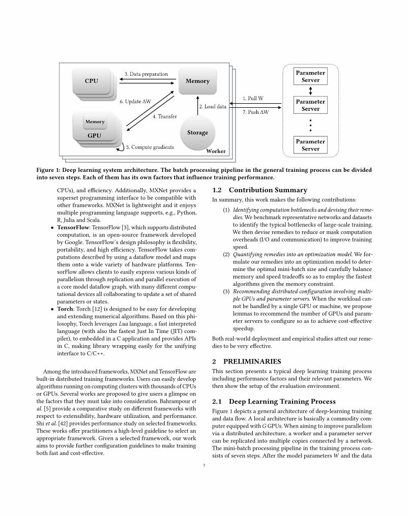
Figure 1: Deep learning system architecture. The batch processing pipeline in the general training process can be dividedinto seven steps. Each of them has its own factors that influence training performance.
CPUs), and efficiency. Additionally, MXNet provides a
superset programming interface to be compatible with
other frameworks. MXNet is lightweight and it enjoys
multiple programming language supports, e.g., Python,
R, Julia and Scala.
• TensorFlow: TensorFlow [3], which supports distributed
computation, is an open-source framework developed
by Google. TensorFlow’s design philosophy is flexibility,
portability, and high efficiency. TensorFlow takes com-
putations described by using a dataflow model and maps
them onto a wide variety of hardware platforms. Ten-
sorFlow allows clients to easily express various kinds of
parallelism through replication and parallel execution of
a core model dataflow graph, with many different compu-
tational devices all collaborating to update a set of shared
parameters or states.
• Torch: Torch [12] is designed to be easy for developing
and extending numerical algorithms. Based on this phi-
losophy, Torch leverages Lua language, a fast interpretedlanguage (with also the fastest Just In Time (JIT) com-
piler), to embedded in a C application and provides APIs
in C, making library wrapping easily for the unifying
interface to C/C++.
Among the introduced frameworks, MXNet and TensorFlow are
built-in distributed training frameworks. Users can easily develop
algorithms running on computing clusters with thousands of CPUs
or GPUs. Several works are proposed to give users a glimpse on
the factors that they must take into consideration. Bahrampour etal. [5] provide a comparative study on different frameworks with
respect to extensibility, hardware utilization, and performance.
Shi et al. [42] provides performance study on selected frameworks.
These works offer practitioners a high-level guideline to select an
appropriate framework. Given a selected framework, our work
aims to provide further configuration guidelines to make training
both fast and cost-effective.
1.2 Contribution SummaryIn summary, this work makes the following contributions:
(1) Identifying computation bottlenecks and devising their reme-dies. We benchmark representative networks and datasets
to identify the typical bottlenecks of large-scale training.
We then devise remedies to reduce or mask computation
overheads (I/O and communication) to improve training
speed.
(2) Quantifying remedies into an optimization model. We for-
mulate our remedies into an optimization model to deter-
mine the optimal mini-batch size and carefully balance
memory and speed tradeoffs so as to employ the fastest
algorithms given the memory constraint.
(3) Recommending distributed configuration involving multi-ple GPUs and parameter servers. When the workload can-
not be handled by a single GPU or machine, we propose
lemmas to recommend the number of GPUs and param-
eter servers to configure so as to achieve cost-effective
speedup.
Both real-world deployment and empirical studies attest our reme-
dies to be very effective.
2 PRELIMINARIESThis section presents a typical deep learning training process
including performance factors and their relevant parameters. We
then show the setup of the evaluation environment.
2.1 Deep Learning Training ProcessFigure 1 depicts a general architecture of deep-learning training
and data flow. A local architecture is basically a commodity com-
puter equipped withG GPUs. When aiming to improve parallelism
via a distributed architecture, a worker and a parameter server
can be replicated into multiple copies connected by a network.
The mini-batch processing pipeline in the training process con-
sists of seven steps. After the model parametersW and the data
3
processing pipeline is initialized, the training process repeats until
all training data is seen.
(1) Parameter refresh. In distributed training, the latest copy
of model parametersW is pulled from parameter servers
at the beginning of each mini-batch processing.W is then
loaded onto GPU memory. A distributed environment
consists of Nw workers and Nps parameter servers for
managing shared parameters.
(2) Data loading. A subset of the X training instances called
mini-batch of size Xmini is loaded from the persistent
storage to the main memory.
(3) Data preparation. Xmini instances are transformed into
the required input format. These instances may be aug-
mented to mitigate the over-fitting problem and enrich
sample diversity.
(4) Host to GPU transfer. The mini-batch is loaded onto the
memory of a GPU. If G GPUs are employed, G different
mini-batches are loaded onto G GPUs.
(5) GPU processing. Required computations including matrix
multiplication and convolution are performed onG GPUs
for the gradients against the given mini-batch.
(6) Parameter update. The delta ∆W is derived from the gra-
dients and applied to the previous version ofW in main
or GPU memory.
(7) Distributed update. The parameter updates are sent to
parameter servers when distributed machines are config-
ured.
Among the seven steps, step 5 performs computation, and the
other steps that cannot be hidden behind step 5 are considered as
overheads. The larger fraction of the time which those overhead
steps take, the less effective parallelism can achieve. Therefore,
our tasks are minimizing overhead time and hiding overheads via
pipelining as much as possible. The remainder of this paper is to
demonstrate how the following parameters can be carefully tuned
to achieve such goals, organized into four sections. In section 3.1,
we provide a procedure to recommend a mini-batch size that
leads to maximum training performance. Section 3.2 provides an
in-depth analysis on training in a multi-GPU environment. We
provide a lemma to estimate the number of GPUs G for a desired
factor of speedup. The increase of GPU number not only improves
performance speedup, but also induces communication overheads
between GPUs. We’ll also discuss how to alleviate the impacts
of these overheads. In section 3.3, we address issues involving
distributed workers. When the training system scales horizontally,
we need an extra cluster to manage the parameters in addition to
training hosts in the distributed environment. The communication
between training hosts and parameter servers is an overhead that
could seriously degrade training speedup. We propose a scheme
to estimate the number of parameter servers Nps whose network
capacity is Bps .
2.2 Evaluation EnvironmentWe set up our evaluation environment with Elastic Compute Cloud
(EC2) of Amazon Web Services (AWS)2. All experiments run on
EC2 P2 instances equipped with NVIDIA Tesla K80 Accelerators
which contain a pair of NVIDIA GK210 GPUs. Each GPU pro-
vides 12 GB memory and 2, 496 parallel processing cores. The
CPU is a customized version of Intel Broadwell processor running
at 2.7 GHz. Table 1 shows hardware configurations of P2 type
instances3. To avoid unexpected GPU clock rate adjustment in
our experiments, we disable GPU autoboost function.
Table 1: AWS P2 instances
Instance #GPU GPU Mem. Network
p2.xlarge 1 12 GB High
p2.8xlarge 8 96 GB 10 Gbps
p2.16xlarge 16 192 GB 20 Gbps
We perform experiments and demonstrate our ideas by MXNet
and TensorFlow. Virtual machines are launched from Amazon
deep learning AMI (Amazon Machine Image) v2.1 preloaded with
NVIDIA CUDA toolkit v7.5 and cuDNN v5.1. We conduct experi-
ments on the ILSVRC-2012 dataset, the subset of ImageNet [16]
containing 1, 000 categories and 1.2 million images on SSD. The
other set containing 50, 000 labeled images is used as validation
data.
3 CONFIGURATION OF HIGHPERFORMANCE TRAINING SYSTEM
We study configuration in three incremental steps, starting from a
single GPU, then expanding our benchmarking to multiple GPUs,
and finally to distributed nodes where each node consists of multi-
GPUs. Each of these three steps focuses on analyzing one system
configuration.
In the single GPU study, we analyze how the mini-batch size
Xmini can be decided to achieve fast training speed. Most prior
studies only consider tuning Xmini algorithmically, that is, select-
ing a size that can achieve fast convergence. However, taking the
minimum number of epochs to reach convergence does not di-
rectly translate to shortest training time. In Section 3.1 we provide
system analysis to determine Xmini and solve optimized mini-
batch selection with integer linear programming.
As multiple GPUs are employed to conduct training, data mov-
ing is the major bottleneck, which caps the speedup performance
according to Amdahl’s law. Therefore, to be cost-effective, we
should not use more GPUs when speedup improvement has satu-
rated. Section 3.2 presents a systematic procedure to estimate an
effective number of GPUs G.
2GPU instances on Google Compute Engine (GCE) do not support GPU peer-to-peer
access, and hence we will defer our GCE experiments till such support is available.
3p2.16xlarge is not used in our experiments because it does not support full GPU-to-
GPU communication which introduces one more variable in our multi-GPU experi-
ments.
4
When training is conducted in a distributed environment, we
further study communication overhead. Section 3.3 depicts the
distributed training process and provides a lemma to estimate the
required number of parameter servers in a cost-effective system
configuration.
3.1 Training on single GPU instanceIn this section, we first point out the common performance pitfalls
in designing neural networks. We illustrate that the setting of
mini-batch size is the primary factor that determines training
speed. We then formulate selecting the mini-batch size Xmini as
an optimization problem and provide a procedure to solve for
Xmini that can achieve fastest training speed.
3.1.1 Identifying System Issues. Most neural networks are ini-
tially designed according to some heuristics. Researchers may not
have the full picture about their model’s feasibility, convergence
quality, and prediction quality unless they conducted some experi-
ments. During the experimental process, various hyper-parameter
values may be tested exhaustively by a trial-and-error process.
According to our own experience, it is typically unknown at the be-
ginning to know how long it would take to run a round of training
job, let alone configure a cost-effective system that can maximize
training speed. A suboptimal system configuration can lead to
excessive execution time because of encountering the following
issues:
• Shortage of GPU memory space. A GPU cannot commence
computation without the data, including model parame-
ters, gradients, computation workspace, etc, being loaded
into GPU memory. A neural network designed without
system knowledge may require more memory capacity
than available memory. This excessive memory use may
cause unnecessary thrashing and prolong training time.
• Ineffective tradeoff between speed and memory. Deep learn-ing frameworks may execute operations of a training task
by using different algorithms, which have different speed
and memory-use trade-offs. The selection of using which
algorithm is a layer-dependent decision. The selection
factors include input data size, layer parameters, mini-
batch size, and available GPU memory space. Consider
the convolution operation as an example. An FFT-based
algorithm runs faster than a GEMM-based one but it re-
quires more memory. The training speedmay be degraded
when a large Xmini exhausts memory capacity in order
to run a faster FFT-based algorithm. Thus, when tuning
factors mentioned above, we should consider the impact
on memory consumption because the memory budget
affects the selection of algorithm.
Both training convergence and training speed can be decided by
mini-batch size. In other words, selecting a good mini-batch size,
one must examine from both the algorithmic and system aspects.
From the algorithmic aspect, the mini-batch size is suggested to be
larger than the number of output classes and a mini-batch contains
at least one sample from each class [25]. The diversified training
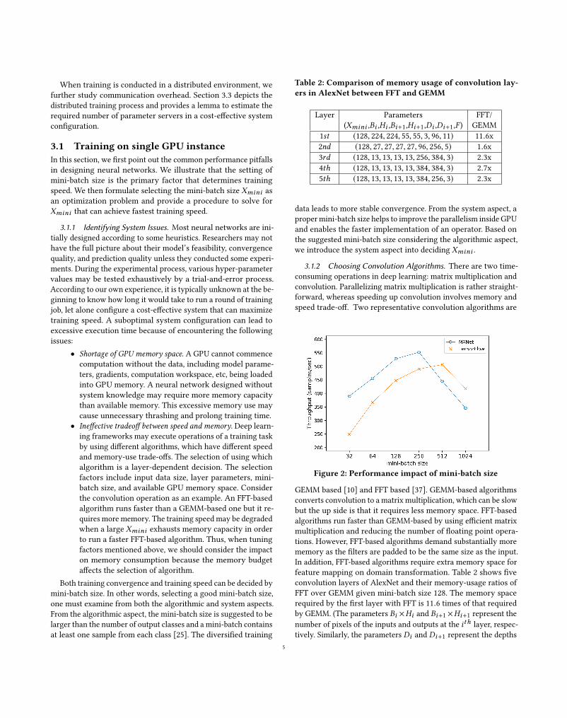
Table 2: Comparison of memory usage of convolution lay-ers in AlexNet between FFT and GEMM
Layer Parameters FFT/
(Xmini ,Bi ,Hi ,Bi+1,Hi+1,Di ,Di+1,F ) GEMM
1st (128, 224, 224, 55, 55, 3, 96, 11) 11.6x
2nd (128, 27, 27, 27, 27, 96, 256, 5) 1.6x
3rd (128, 13, 13, 13, 13, 256, 384, 3) 2.3x
4th (128, 13, 13, 13, 13, 384, 384, 3) 2.7x
5th (128, 13, 13, 13, 13, 384, 256, 3) 2.3x
data leads to more stable convergence. From the system aspect, a
propermini-batch size helps to improve the parallelism inside GPU
and enables the faster implementation of an operator. Based on
the suggested mini-batch size considering the algorithmic aspect,
we introduce the system aspect into deciding Xmini .
3.1.2 Choosing Convolution Algorithms. There are two time-
consuming operations in deep learning: matrix multiplication and
convolution. Parallelizing matrix multiplication is rather straight-
forward, whereas speeding up convolution involves memory and
speed trade-off. Two representative convolution algorithms are
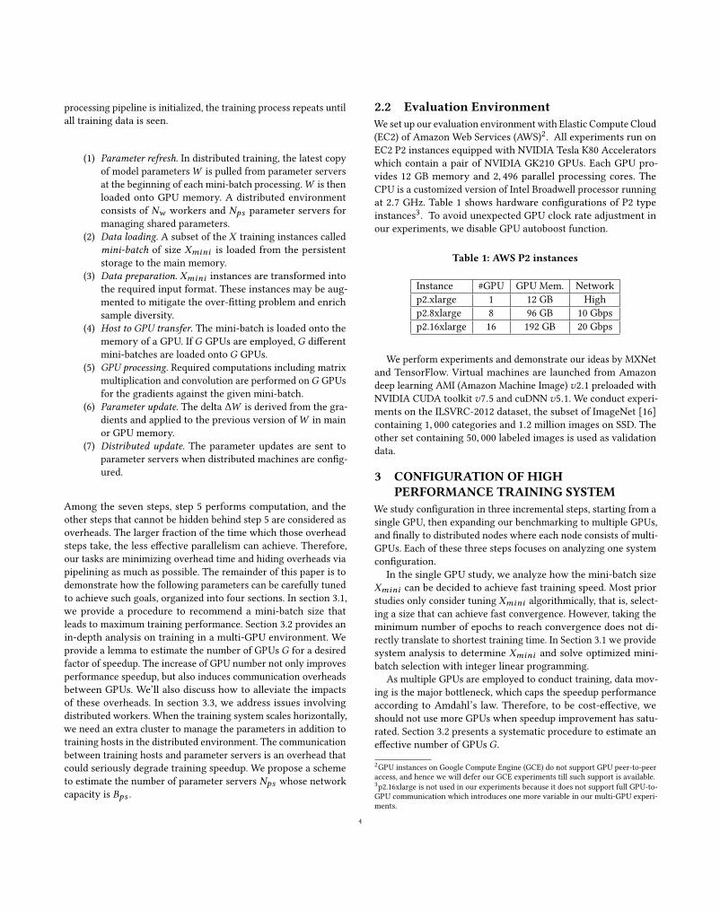
Figure 2: Performance impact of mini-batch size
GEMM based [10] and FFT based [37]. GEMM-based algorithms
converts convolution to a matrix multiplication, which can be slow
but the up side is that it requires less memory space. FFT-based
algorithms run faster than GEMM-based by using efficient matrix
multiplication and reducing the number of floating point opera-
tions. However, FFT-based algorithms demand substantially more
memory as the filters are padded to be the same size as the input.
In addition, FFT-based algorithms require extra memory space for
feature mapping on domain transformation. Table 2 shows five
convolution layers of AlexNet and their memory-usage ratios of
FFT over GEMM given mini-batch size 128. The memory space
required by the first layer with FFT is 11.6 times of that required
by GEMM. (The parameters Bi ×Hi and Bi+1 ×Hi+1 represent the
number of pixels of the inputs and outputs at the ith layer, respec-
tively. Similarly, the parameters Di and Di+1 represent the depths
5
of the inputs and outputs at the ith , respectively. The parameter
F represents the size of filters.)
To further understand the impact of Xmini , we experimented
with MXNet and TensorFlow, and plot system throughout (y-axis)versus Xmini (x-axis) in Figure 2. Although different frameworks
may yield different throughputs, the trend remains the same, that
is, the system throughput degrades once after Xmini reaches a
threshold. The reason why the throughput drops is that MXNet
and TensorFlow choose to run a slower convolution algorithm due
to the constrained free memory caused by the increased Xmini .
How to determine the optimal Xmini? We next formulate the
problem of determining Xmini as an optimization problem.
3.1.3 Optimizing Mini-batch Size. In order to formulate the
problem of determining Xmini , we first define a memory con-
straintMbound , which is built into the later optimization formulas
for Xmini . During our formulation, most of the symbols follow in
the same fashion of [2].
DerivingMbound .
We assume that a CNN such as AlexNet [32] consists of two ma-
jor components: feature extraction and classification. Further, we
assume that the feature extraction part comprises ofn layers wherestacked convolution layers are optionally followed by pooling lay-
ers, and the classification part consists ofm fully-connected layers.
We use Bi ×Hi ×Di and Bi+1×Hi+1×Di+1 where i ∈ {0, 1, . . . ,n}to represent the sizes of inputs and outputs of convolution layers
(or pooling layers), respectively. In particular, the size B0×H0×D0
represents the size of input data. If we take training AlexNet on the
ImageNet [16] as the example, B0×H0×D0 is equal to 224×224×3.For the ith layer of convolution and pooling layers, we denote
its spatial extent (i.e. the size of filters) as Fi , its stride as Si , itsamount of padding as Pi , and its number of filters as Ki . Please
note that if the ith layer is a pooling layer, its Ki is equal to zero,
i.e. Ki = 0. Thus, the inputs and outputs in the feature extraction
part have the following relations:
Bi+1 = (Bi − Fi+1 + 2Pi+1)/Si+1 + 1,Hi+1 = (Hi − Fi+1 + 2Pi+1)/Si+1 + 1,and
Di+1 =
{Ki+1, if (i + 1)th layer is convolution layer
Di , if (i + 1)th layer is pooling layer
.
(1)
The memory allocated for the feature extraction part of CNNs
includes the input data, outputs (i.e. feature maps) of all the layers,
model parameters, and gradients. We assume that all the values
are stored by using single precision floating point (32bits). Based
on the aforementioned notations and Equation (1), the memory
usage for the input data and outputs of all layers in the feature
extraction part can be calculated as follows:
MFM =
n∑i=0
Bi × Hi × Di × Xmini × 32 . (2)
Regarding the model parameters, there are two kinds of param-
eters: weights and biases. Though the biases are often omitted
for simplicity in the literature, we take them into account here in
order to estimate the memory usage precisely. Besides, we assume
that the size of the gradients is twice as the size of the model pa-
rameters4. Thus, we can derive the memory usage for the model
parameters and their related gradients by the following equation:
MMP =
n∑i=1
Fi × Fi × Di−1 × Ki × 3 × 32+ (weiдhts)
n∑i=1
Ki × 3 × 32 (biases) .(3)
Furthermore, the memory allocated for the classification part of
CNNs contains the outputs of all neurons and model parameters.
We useLj where j ∈ {1, . . . ,m} to denote the number of neurons at
jth layer. Again, we make the same assumption that the size of the
gradients is twice as the size of the model parameters. Therefore,
the memory usage for the classification part of CNNs is as follows:
MC =
m∑j=1
Lj × 32+ (outputs)
m−1∑j=1
Lj × Lj+1 × 3 × 32+ (weiдhts)
(m − 1) × 3 × 32 (biases) .
(4)
According to Equations (2) to (4), the memory constraintMboundcan be approximately determined by the following equation:
Mbound = MGPU −MFM −MMP −MC , (5)
whereMGPU is the total memory of a GPU in terms of bits.
Deriving Xmini .
Assuming that there are p kinds of convolution algorithms,
and q layers in the CNN. (In the case that we have illustrated so
far, p = 2. Other choices of convolution algorithms can be Wino-
grad minimal convolution algorithm [33], Strassen algorithm [13],
fbfft [44], etc.) The parameter xk,l ∈ {0, 1} represents whether thekth layer uses the lth convolution algorithm or not. When xk,l is
evaluated to 1, it means that the kth layer uses the lth algorithm
to compute convolution. The value Tk,l is the time consumption
at the kth layer for the lth algorithm. The valueMk,l is the mem-
ory consumption at the kth layer for the lth algorithm. Thus, the
problem of determining Xmini can be formulated an optimization
problem as follows:
min
q∑k=1
p∑l=1
xk,l ×Tk,l
s .t .
q∑k=1
p∑l=1
xk,l ×Mk,l ≤ Mbound and
∀kp∑l=1
xk,l = 1,
(6)
4For each training instance, we need to store the gradients of all model parameters.
The aggregated gradients of all model parameters are also required for a specific
batch.
6
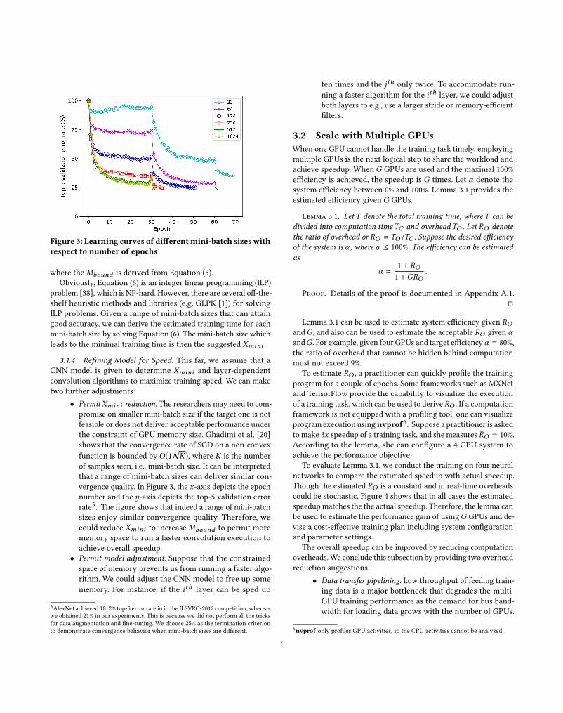
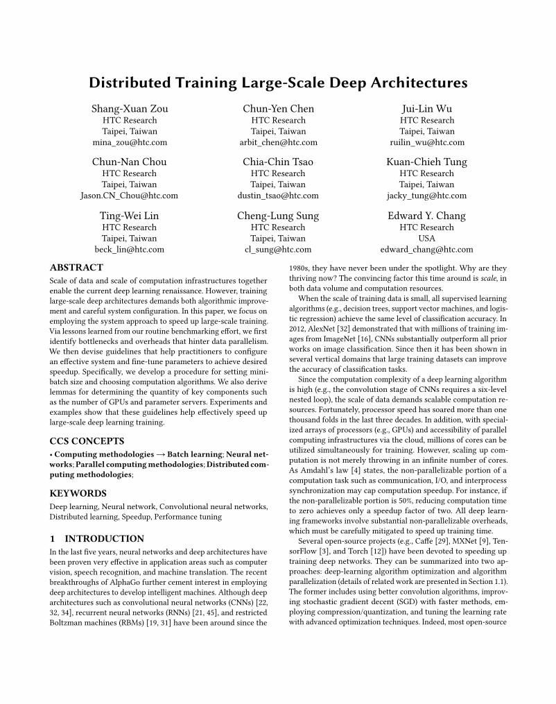
Figure 3: Learning curves of differentmini-batch sizes withrespect to number of epochs
where theMbound is derived from Equation (5).
Obviously, Equation (6) is an integer linear programming (ILP)
problem [38], which is NP-hard. However, there are several off-the-
shelf heuristic methods and libraries (e.g. GLPK [1]) for solving
ILP problems. Given a range of mini-batch sizes that can attain
good accuracy, we can derive the estimated training time for each
mini-batch size by solving Equation (6). The mini-batch size which
leads to the minimal training time is then the suggested Xmini .
3.1.4 Refining Model for Speed. This far, we assume that a
CNN model is given to determine Xmini and layer-dependent
convolution algorithms to maximize training speed. We can make
two further adjustments:
• PermitXmini reduction. The researchers may need to com-
promise on smaller mini-batch size if the target one is not
feasible or does not deliver acceptable performance under
the constraint of GPU memory size. Ghadimi et al. [20]
shows that the convergence rate of SGD on a non-convex
function is bounded by O(1/√K), where K is the number
of samples seen, i.e., mini-batch size. It can be interpreted
that a range of mini-batch sizes can deliver similar con-
vergence quality. In Figure 3, the x-axis depicts the epochnumber and the y-axis depicts the top-5 validation error
rate5. The figure shows that indeed a range of mini-batch
sizes enjoy similar convergence quality. Therefore, we
could reduce Xmini to increaseMbound to permit more
memory space to run a faster convolution execution to
achieve overall speedup.
• Permit model adjustment. Suppose that the constrainedspace of memory prevents us from running a faster algo-
rithm. We could adjust the CNN model to free up some
memory. For instance, if the ith layer can be sped up
5AlexNet achieved 18.2% top-5 error rate in in the ILSVRC-2012 competition, whereas
we obtained 21% in our experiments. This is because we did not perform all the tricks
for data augmentation and fine-tuning. We choose 25% as the termination criterion
to demonstrate convergence behavior when mini-batch sizes are different.
ten times and the jth only twice. To accommodate run-
ning a faster algorithm for the ith layer, we could adjust
both layers to e.g., use a larger stride or memory-efficient
filters.
3.2 Scale with Multiple GPUsWhen one GPU cannot handle the training task timely, employing
multiple GPUs is the next logical step to share the workload and
achieve speedup. When G GPUs are used and the maximal 100%
efficiency is achieved, the speedup is G times. Let α denote the
system efficiency between 0% and 100%. Lemma 3.1 provides the
estimated efficiency given G GPUs.
Lemma 3.1. Let T denote the total training time, where T can bedivided into computation time TC and overhead TO . Let RO denotethe ratio of overhead or RO = TO /TC . Suppose the desired efficiencyof the system is α , where α ≤ 100%. The efficiency can be estimatedas
α =1 + RO1 +GRO
.
Proof. Details of the proof is documented in Appendix A.1.
□
Lemma 3.1 can be used to estimate system efficiency given ROandG , and also can be used to estimate the acceptable RO given αandG . For example, given four GPUs and target efficiencyα = 80%,
the ratio of overhead that cannot be hidden behind computation
must not exceed 9%.
To estimate RO , a practitioner can quickly profile the training
program for a couple of epochs. Some frameworks such as MXNet
and TensorFlow provide the capability to visualize the execution
of a training task, which can be used to derive RO . If a computation
framework is not equipped with a profiling tool, one can visualize
program execution usingnvprof6. Suppose a practitioner is askedto make 3x speedup of a training task, and she measures RO = 10%.
According to the lemma, she can configure a 4 GPU system to
achieve the performance objective.
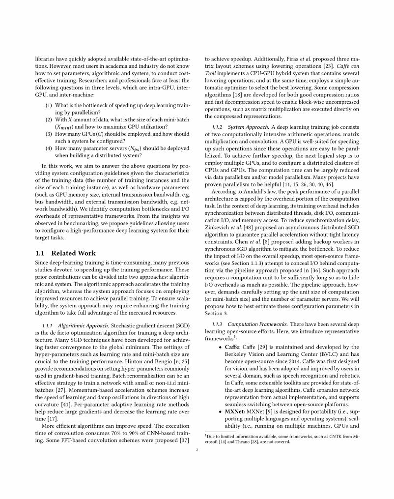
To evaluate Lemma 3.1, we conduct the training on four neural
networks to compare the estimated speedup with actual speedup.
Though the estimated RO is a constant and in real-time overheads
could be stochastic, Figure 4 shows that in all cases the estimated
speedupmatches the the actual speedup. Therefore, the lemma can
be used to estimate the performance gain of usingG GPUs and de-
vise a cost-effective training plan including system configuration
and parameter settings.
The overall speedup can be improved by reducing computation
overheads.We conclude this subsection by providing two overhead
reduction suggestions.
• Data transfer pipelining. Low throughput of feeding train-
ing data is a major bottleneck that degrades the multi-
GPU training performance as the demand for bus band-
width for loading data grows with the number of GPUs.
6nvprof only profiles GPU activities, so the CPU activities cannot be analyzed.
7
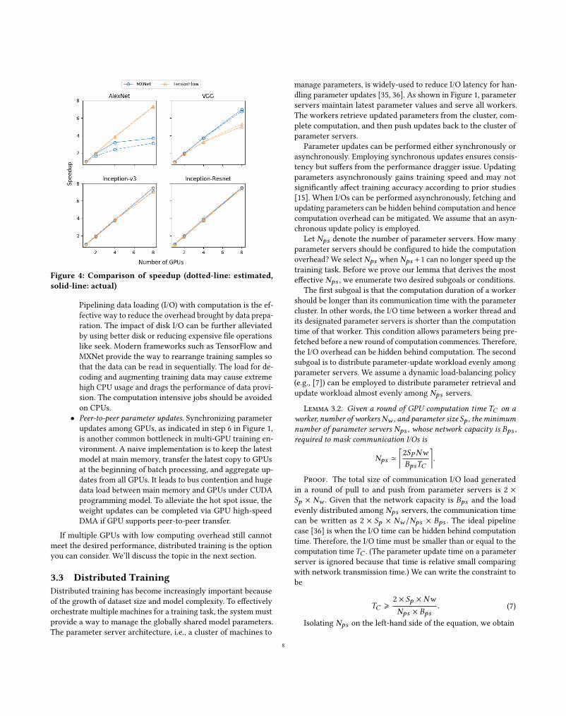
Figure 4: Comparison of speedup (dotted-line: estimated,solid-line: actual)
Pipelining data loading (I/O) with computation is the ef-
fective way to reduce the overhead brought by data prepa-
ration. The impact of disk I/O can be further alleviated
by using better disk or reducing expensive file operations
like seek. Modern frameworks such as TensorFlow and
MXNet provide the way to rearrange training samples so
that the data can be read in sequentially. The load for de-
coding and augmenting training data may cause extreme
high CPU usage and drags the performance of data provi-
sion. The computation intensive jobs should be avoided
on CPUs.
• Peer-to-peer parameter updates. Synchronizing parameter
updates among GPUs, as indicated in step 6 in Figure 1,
is another common bottleneck in multi-GPU training en-
vironment. A naive implementation is to keep the latest
model at main memory, transfer the latest copy to GPUs
at the beginning of batch processing, and aggregate up-
dates from all GPUs. It leads to bus contention and huge
data load between main memory and GPUs under CUDA
programming model. To alleviate the hot spot issue, the
weight updates can be completed via GPU high-speed
DMA if GPU supports peer-to-peer transfer.
If multiple GPUs with low computing overhead still cannot
meet the desired performance, distributed training is the option
you can consider. We’ll discuss the topic in the next section.
3.3 Distributed TrainingDistributed training has become increasingly important because
of the growth of dataset size and model complexity. To effectively
orchestrate multiple machines for a training task, the system must
provide a way to manage the globally shared model parameters.
The parameter server architecture, i.e., a cluster of machines to
manage parameters, is widely-used to reduce I/O latency for han-
dling parameter updates [35, 36]. As shown in Figure 1, parameter
servers maintain latest parameter values and serve all workers.
The workers retrieve updated parameters from the cluster, com-
plete computation, and then push updates back to the cluster of
parameter servers.
Parameter updates can be performed either synchronously or
asynchronously. Employing synchronous updates ensures consis-
tency but suffers from the performance dragger issue. Updating
parameters asynchronously gains training speed and may not
significantly affect training accuracy according to prior studies
[15]. When I/Os can be performed asynchronously, fetching and
updating parameters can be hidden behind computation and hence
computation overhead can be mitigated. We assume that an asyn-
chronous update policy is employed.
Let Nps denote the number of parameter servers. How many
parameter servers should be configured to hide the computation
overhead? We select Nps when Nps +1 can no longer speed up the
training task. Before we prove our lemma that derives the most
effective Nps , we enumerate two desired subgoals or conditions.
The first subgoal is that the computation duration of a worker
should be longer than its communication time with the parameter
cluster. In other words, the I/O time between a worker thread and
its designated parameter servers is shorter than the computation
time of that worker. This condition allows parameters being pre-
fetched before a new round of computation commences. Therefore,
the I/O overhead can be hidden behind computation. The second
subgoal is to distribute parameter-update workload evenly among
parameter servers. We assume a dynamic load-balancing policy
(e.g., [7]) can be employed to distribute parameter retrieval and
update workload almost evenly among Nps servers.
Lemma 3.2. Given a round of GPU computation time TC on aworker, number of workersNw , and parameter size Sp , the minimumnumber of parameter servers Nps , whose network capacity is Bps ,required to mask communication I/Os is
Nps ≃⌈2SPNw
BpsTC
⌉.
Proof. The total size of communication I/O load generated
in a round of pull to and push from parameter servers is 2 ×Sp × Nw . Given that the network capacity is Bps and the load
evenly distributed among Nps servers, the communication time
can be written as 2 × Sp × Nw /Nps × Bps . The ideal pipeline
case [36] is when the I/O time can be hidden behind computation
time. Therefore, the I/O time must be smaller than or equal to the
computation timeTC . (The parameter update time on a parameter
server is ignored because that time is relative small comparing
with network transmission time.) We can write the constraint to
be
TC ⩾2 × Sp × Nw
Nps × Bps. (7)
Isolating Nps on the left-hand side of the equation, we obtain
8
Nps ⩾2SpNw
TCBps. (8)
□
Lemma 3.2 suggests a back-of-the-envelop estimate on Npsgiven two ideal conditions. When the conditions do not hold,
more parameter servers should be employed to be able to mask
I/O overhead. Three measures are recommended:
(1) IncreaseTC . When workload cannot be evenly distributed,
the computation time should be longer to mask most
I/Os. Therefore, a good strategy is to maintain a large
TC . In other words, having a larger mini-batch size when
the memory capacity permits is helpful. Besides, a larger
mini-batch leads to less number of parameter updates and
improves overall performance.
(2) Improve Bps . Increasing channel bandwidth can reduce
I/O time. Insufficient bandwidth of the communication
channelmay throttle the training performance. TakeAlexNet
as an example, pushing parameter updates produces around
180MB network traffic, which exceeds the capacity of com-
monly used 1Gbit Ethernet. Thus, high speed networking
is highly recommended when applying distributed train-
ing.
(3) Balance workload. Prior works [7, 36] propose effectivedata placement methods to balance dynamic workload.
Such load balancing schemes can avoid I/O bottlenecks,
and lead to overall overhead reduction.
4 CONCLUDING REMARKSIn this work, we investigated typical deep learning frameworks
running on representative deep learning models and datasets.
From analyses, we studied the computation bottlenecks in single-
GPU, multi-GPU and distributed configurations. Furthermore, we
derived the back-of-the-envelope estimation for the GPU num-
ber to configure a training system, given a budget or deadline.
Finally, for distributed training, we suggested a formula for es-
timating the number of parameter servers to be configured to
reduce communication overhead.
AlphaGo showed that more training data can only be help-
ful towards improving machine intelligence and competitiveness.
Recently, Residual Neural Networks [24, 43] shows that in both
theory and practice, more layers of neural networks correlates to a
higher achieved accuracy by a trained classifier. At a 2016 machine
learning workshop [39], Andrew Ng presented that the traditional
biases and variance tradeoff have not appeared in training large-
scale deep architectures. In other words, the larger the scale, the
better suited the architecture is for improving the intelligence of
a “machine”.
This “larger the better” conclusion certainly demands that data-
base and machine learning communities devise data management
and data mining systems that can handle an ever increasing work-
load. We foresee that not only will algorithmic research continue
flourishing, but system research and development will as well.
Already we have seen that GPU vendors are enhancing distributed
GPU implementations. Advances in interconnected technology
and implementation will help reduce both I/O overhead in data
loading and in parameter updates.
In this work, we provided practical guidelines to facilitate prac-
titioners the configuration of a system to speed up training perfor-
mance. Our future work will focus on effectively managing such
large-scale training systems to achieve both high accuracy and
cost-effectiveness in three specific areas:
• Flexibility. Prior work [47] provided a flexibility to work
with any compatible open-source frameworks. For ex-
ample, we expect to simultaneously work with multiple
frameworks such as MXNet and TensorFlow to complete
a large-scale training task running on Azure, AWS, GCE,
and other available commercial clouds.
• Scalability and elasticity. In addition to the parameter esti-
mation performed in this work, we will research dynamic
schemes to adjust allocation and scheduling parameters
according to the dynamic workload nature of distributed
systems.
• Ease of management. We plan to devise tools with the
good user experience for monitoring and managing the
training system.
A APPENDICESA.1 Proof of Lemma 3.1According to Amdahl’s law, givenG GPUs and the fraction of the
execution time of the task that can be parallelized P , the theoreticalspeedup is
1
(1−P )+ PG. Themaximum speedupG can not be achieved
if there are parts cannot be parallelized. Thus:
αG =1
(1 − P) + PG
(9)
P can be expressed as:
P =TCT=
TCTC +TO
(10)
Substituting P into equation 9 yields:
TOTC=
1 − α
αG − 1
(11)
Then:
RO =1 − α
αG − 1
(12)
By rearranging equation 12, α can be expressed in terms of Gand RO as follows:
α =1 + RO1 +GRO
(13)
REFERENCES[1] 2012. GNU Linear Programming Kit. https://www.gnu.org/software/glpk/.
(2012).
[2] 2017. CS231n Convolutional neural network for visual recognition. http:
//cs231n.github.io/. (2017).
9
[3] Martın Abadi, Ashish Agarwal, Paul Barham, Eugene Brevdo, Zhifeng Chen,
Craig Citro, Greg S Corrado, Andy Davis, Jeffrey Dean, Matthieu Devin, and
others. 2015. TensorFlow: Large-scale machine learning on heterogeneous
systems, 2015. Software available from tensorflow. org 1 (2015).
[4] Gene M Amdahl. 1967. Validity of the single processor approach to achieving
large scale computing capabilities. In Proceedings of the April 18-20, 1967, springjoint computer conference. ACM, 483–485.
[5] Soheil Bahrampour, Naveen Ramakrishnan, Lukas Schott, and Mohak Shah.
2015. Comparative Study of Deep Learning Software Frameworks. arXiv.org(Nov. 2015). arXiv:1511.06435v3
[6] Yoshua Bengio. 2012. Practical recommendations for gradient-based training of
deep architectures. In Neural Networks: Tricks of the Trade. Springer, 437–478.[7] Edward Chang, Hector Garcia-Molina, and Chen Li. 1998. 2D BubbleUp: Man-
aging Parallel Disks for Media Servers. Technical Report. Stanford InfoLab.
[8] Jianmin Chen, Rajat Monga, Samy Bengio, and Rafal Jozefowicz. 2016. Revisit-
ing Distributed Synchronous SGD. arXiv preprint arXiv:1604.00981 (2016).[9] Tianqi Chen, Mu Li, Yutian Li, Min Lin, Naiyan Wang, Minjie Wang, Tianjun
Xiao, Bing Xu, Chiyuan Zhang, and Zheng Zhang. 2015. Mxnet: A flexible and
efficient machine learning library for heterogeneous distributed systems. arXivpreprint arXiv:1512.01274 (2015).
[10] Sharan Chetlur, Cliff Woolley, Philippe Vandermersch, Jonathan Cohen, John
Tran, Bryan Catanzaro, and Evan Shelhamer. 2014. cuDNN: Efficient Primitives
for Deep Learning. CoRR abs/1410.0759 (2014). http://arxiv.org/abs/1410.0759
[11] Trishul M Chilimbi, Yutaka Suzue, Johnson Apacible, and Karthik Kalyanara-
man. 2014. Project Adam: Building an Efficient and Scalable Deep Learning
Training System.. In OSDI, Vol. 14. 571–582.[12] Ronan Collobert, Koray Kavukcuoglu, and Clément Farabet. 2011. Torch7: A
matlab-like environment for machine learning. EPFL-CONF-192376 (2011).
[13] Jason Cong and Bingjun Xiao. 2014. Minimizing computation in convolutional
neural networks. In International Conference on Artificial Neural Networks.Springer, 281–290.
[14] W J Dally. CNTK: An Embedded Language for Circuit Description, Dept. of
Computer Science, California Institute of Technology, Display File.
[15] Jeffrey Dean, Greg Corrado, Rajat Monga, Kai Chen, Matthieu Devin, Mark
Mao, Andrew Senior, Paul Tucker, Ke Yang, Quoc V Le, and others. 2012. Large
scale distributed deep networks. (2012), 1223–1231.
[16] J. Deng, W. Dong, R. Socher, L.-J. Li, K. Li, and L. Fei-Fei. 2009. ImageNet: A
Large-Scale Hierarchical Image Database. In CVPR09.[17] John Duchi, Elad Hazan, and Yoram Singer. 2011. Adaptive subgradient methods
for online learning and stochastic optimization. Journal of Machine LearningResearch 12, Jul (2011), 2121–2159.
[18] Ahmed Elgohary, Matthias Boehm, Peter J Haas, Frederick R Reiss, and Berthold
Reinwald. 2016. Compressed linear algebra for large-scale machine learning.
Proceedings of the VLDB Endowment 9, 12 (2016), 960–971.[19] Asja Fischer and Christian Igel. 2012. An introduction to restricted Boltzmann
machines. In Iberoamerican Congress on Pattern Recognition. Springer, 14–36.[20] Saeed Ghadimi and Guanghui Lan. 2013. Stochastic first-and zeroth-order
methods for nonconvex stochastic programming. SIAM Journal on Optimization23, 4 (2013), 2341–2368.
[21] A Graves and N Jaitly. 2014. Towards End-To-End Speech Recognition with
Recurrent Neural Networks. ICML (2014).
[22] Alex Graves, Abdel-rahman Mohamed, and Geoffrey Hinton. 2013. Speech
Recognition with Deep Recurrent Neural Networks. arXiv.org (March 2013).
arXiv:1303.5778v1
[23] Stefan Hadjis, Firas Abuzaid, Ce Zhang, and Christopher Ré. 2015. Caffe
con Troll: Shallow Ideas to Speed Up Deep Learning. arXiv.org (April 2015).
arXiv:1504.04343v2
[24] Kaiming He, Xiangyu Zhang, Shaoqing Ren, and Jian Sun. 2016. Deep residual
learning for image recognition. (2016), 770–778.
[25] Geoffrey Hinton. 2010. A practical guide to training restricted Boltzmann
machines. Momentum 9, 1 (2010), 926.
[26] Forrest N Iandola, Matthew W Moskewicz, Khalid Ashraf, and Kurt Keutzer.
2016. FireCaffe - Near-Linear Acceleration of Deep Neural Network Training
on Compute Clusters. CVPR (2016), 2592–2600.
[27] Sergey Ioffe. 2017. Batch Renormalization: Towards ReducingMinibatch Depen-
dence in Batch-Normalized Models. arXiv.org (Feb. 2017). arXiv:1702.03275v1
[28] B James, B Olivier, B Frédéric, L Pascal, and P Razvan. Theano: a CPU and GPU
math expression compiler.
[29] Yangqing Jia, Evan Shelhamer, Jeff Donahue, Sergey Karayev, Jonathan Long,
Ross Girshick, Sergio Guadarrama, and Trevor Darrell. 2014. Caffe: Convo-
lutional Architecture for Fast Feature Embedding. In Proceedings of the 22NdACM International Conference on Multimedia. 675–678.
[30] Alex Krizhevsky. 2014. One weird trick for parallelizing convolutional neural
networks. arXiv preprint arXiv:1404.5997 (2014).
[31] Alex Krizhevsky, Geoffrey E Hinton, and others. 2010. Factored 3-way restricted
boltzmann machines for modeling natural images. (2010), 621–628.
[32] Alex Krizhevsky, Ilya Sutskever, and Geoffrey E. Hinton. 2012. ImageNet Classi-
fication with Deep Convolutional Neural Networks. InAdvances in Neural Infor-mation Processing Systems 25, F. Pereira, C. J. C. Burges, L. Bottou, and K. Q.Wein-
berger (Eds.). Curran Associates, Inc., 1097–1105. http://papers.nips.cc/paper/
4824-imagenet-classification-with-deep-convolutional-neural-networks.pdf
[33] Andrew Lavin and Scott Gray. 2016. Fast algorithms for convolutional neural
networks. In Proceedings of the IEEE Conference on Computer Vision and PatternRecognition. 4013–4021.
[34] Y LeCun, L Bottou, and Y Bengio. 1998. Gradient-based learning applied to
document recognition. Proc. IEEE 86, 11, 2278–2324.
[35] Mu Li, David G Andersen, Jun Woo Park, Alexander J Smola, Amr Ahmed,
Vanja Josifovski, James Long, Eugene J Shekita, and Bor-Yiing Su. 2014. Scaling
Distributed Machine Learning with the Parameter Server. OSDI (2014).[36] Zhiyuan Liu, Yuzhou Zhang, Edward Y. Chang, andMaosong Sun. 2011. PLDA+:
Parallel Latent Dirichlet Allocation with Data Placement and Pipeline Process-
ing. ACM Trans. Intell. Syst. Technol. 2, 3, Article 26 (May 2011), 18 pages.
https://doi.org/10.1145/1961189.1961198
[37] Michael Mathieu, Mikael Henaff, and Yann LeCun. 2013. Fast Training of
Convolutional Networks through FFTs. CoRR abs/1312.5851 cs.CV (2013).
[38] George L Nemhauser and Laurence A Wolsey. 1988. Integer programming and
combinatorial optimization. Wiley, Chichester. GL Nemhauser, MWP Savelsbergh,GS Sigismondi (1992). Constraint Classification for Mixed Integer ProgrammingFormulations. COAL Bulletin 20 (1988), 8–12.
[39] Andrew Y. Ng. 2016. The Nuts and Bolts of Machine Learning. (2016). https:
//nips.cc/Conferences/2010/Schedule?showEvent=1986 NIPS Workshop on
Deep Learning and Unsupervised Feature Learning.
[40] Feng Niu, Benjamin Recht, Christopher Ré, and Stephen J Hogwild Wright.
2011. A lock-free approach to parallelizing stochastic gradient descent. arXiv
preprint. arXiv preprint arXiv:1106.5730 (2011).[41] Boris T Polyak. 1964. Somemethods of speeding up the convergence of iteration
methods. U. S. S. R. Comput. Math. and Math. Phys. 4, 5 (1964), 1–17.[42] Shaohuai Shi, Qiang Wang, Pengfei Xu, and Xiaowen Chu. 2016. Benchmark-
ing State-of-the-Art Deep Learning Software Tools. arXiv.org (Aug. 2016).
arXiv:1608.07249v5
[43] Christian Szegedy, Sergey Ioffe, and Vincent Vanhoucke. 2016. Inception-v4,
Inception-ResNet and the Impact of Residual Connections on Learning. CoRRabs/1602.07261 (2016). http://arxiv.org/abs/1602.07261
[44] Nicolas Vasilache, Jeff Johnson, Michael Mathieu, Soumith Chintala, Serkan
Piantino, and Yann LeCun. 2014. Fast convolutional nets with fbfft: A GPU
performance evaluation. arXiv preprint arXiv:1412.7580 (2014).[45] Wojciech Zaremba, Ilya Sutskever, and Oriol Vinyals. 2014. Recurrent Neural
Network Regularization. arXiv.org (Sept. 2014). arXiv:1409.2329v5
[46] Hao Zhang, Zhiting Hu, Jinliang Wei, Pengtao Xie, Gunhee Kim, Qirong Ho,
and Eric Xing. 2015. Poseidon: A system architecture for efficient gpu-based
deep learning on multiple machines. arXiv preprint arXiv:1512.06216 (2015).[47] Z Zheng, W Jiang, GWu, and E Y Chang. 2015. SpeeDO: Parallelizing stochastic
gradient descent for deep convolutional neural network. NIPS Workshop onLearning Systems (2015).
[48] Martin Zinkevich, Markus Weimer, Lihong Li, and Alex J Smola. 2010. Paral-
lelized stochastic gradient descent. (2010), 2595–2603.
10