Architectures for Accelerating Deep Neural Networks

˃ Part 1: Overview of Deep Learning and Computer Architectures for Accelerating DNNsMichaela Blott, Principal Engineer, Xilinx Research

˃ Part 2: Accelerating Inference at the EdgeSong Han, Assistant Professor, MIT

˃ Part 3: Accelerating Training in the CloudWilliam L. Lynch, VP Engineering and Ardavan Pedram, MTS, Cerebras

>> 1

Michaela Blott

Principal Engineer

August 2018

Overview of Deep

Learning and Computer

Architectures for Accelerating

DNNs

>> 2

The Rise of The Machine (Learning Algorithms)

˃ Potential to solve the unsolved problems

Making solar energy economical, reverse engineering the brain (Jeff Dean, Google Brain 2017)

˃ Many difficult ethical questions

Will machines destroy jobs? AI apocalypse?

˃ History has shown: We are going through cycles of inventions followed by society adjustments

All of this has happened before and will happen again (Battlestar Galactica, 2014)

˃ Let’s look at what the technology can do, and how we computer architects can enable it further

1. 2. 3. 4.1800 1900 2000

MechanicalSteam powered

mechanical production

ElectricalMass production

with electrical energy

DigitalAutomated production

VirtualMachine LearningIndustrial Internet

>> 3

Neural Networks

>> 4

A.I. – Machine Learning - Neural Networks

Artificial Intelligence (A.I.)

Computer Vision Pattern Recognition Machine Learning Cognitive Robotics . . .

Linear Regression K-Means Clustering Decision TreesNeural Networks . . .

“machine mimics cognitive functions such as learning and

problem solving”

“Predominantly used ML algorithmMimics the human brain”

“Gives computers the ability to learn without being explicitly

programmed”

>> 5

Convolutional Neural Networks (CNNs)from a computational point of view

˃ CNNs are usually feed forward* computational

graphs constructed from one or more layers

Up to 1000s of layers

˃ Each layer consists of neurons ni which are

interconnected with synapses, associated with

weights wij

˃ Each neuron computes:

Typically linear transform (dot-product of receptive field)

Followed by a non-linear “activation” functionLayer

L0Layer

L1Layer

L2

WeightsW2

WeightsW1

WeightsW0

Inputs Outputs

i0

i1

w00

w12

n0

n1

n2

n0 = Act(w00*i0 + w10*i1)

Synapse with weight wji

Neuron ni

>> 6* With exception of RNNs

Evolution: From Shallow to Deep Learning

HandcraftedFeature

Extraction

LayerLn-1

WeightsWn-1

Inputs Outputs

extract features& encode in a vector

Feed into classifier(Support Vector Machine or similar)

“ShallowLearning”

LayerL0

LayerL1

LayerLn-1

WeightsWn-1

WeightsW1

WeightsW0

Inputs OutputsLayer

L1

WeightsW1

Learn low level to high level features(pixel, edges, textons, parts, objects)

“DeepLearning”

Image: Simon Thorpe

“Hierarchical learning”

“CAT”

>> 7Freely adapted from Yann LeCun and Kurt Keutzer

Convolutional Neural Networks (CNNs)Why are they so popular?

˃ Requires little or no domain expertise

˃ NNs are a “universal approximation function”

˃ If you make it big enough and train it enough

Can outperform humans on specific tasks

˃ Will increasingly replace other

algorithms

unless for example simple rules can describe the problem

˃ Solve problems previously

unsolved by computers

˃ And solve completely unsolved

problems

>> 8

Increasing Range of Applications

>> 9

Computer VisionCNNs

Object Detection Semantic Segmentation Image Classification

Sedan:0.98Motorcycle:0.005Truck:0.005…

Sedan Sedan

Road

(a)Imageclassification (b)Objectdetection (c)Semanticsegmentation

Speech RecognitionRNNs, LSTMs

SpeechRecognition

SpeakerDiarization

Others

Natural Language ProcessingSequence to sequence

Sentiment AnalysisTranslation

Recommender>> 9

GamePlay

Many more emerging…

Popular Neural Networks

>> 10

Computer VisionCNNs

Object Detection Semantic Segmentation Image Classification

Sedan:0.98Motorcycle:0.005Truck:0.005…

Sedan Sedan

Road

(a)Imageclassification (b)Objectdetection (c)Semanticsegmentation

Speech RecognitionRNNs, LSTMs

SpeechRecognition

SpeakerDiarization

Others

Natural Language ProcessingSequence to sequence

Sentiment AnalysisTranslation

Recommender>> 10

GamePlay

ResNet50, VGG, AlexNet, InceptionV3 Faster R-CNN,

Yolo9000, YoloV2Mask-R-CNN,

SSD

DeepSpeech2

Seq2Seq, Transformer

Seq-CNN

NCFMiniGo,

DeepQ, A3C

Adopted from MLPerf, Fathom, TDP

Training

Process for a machine to learn by

optimizing models (weights) from labeled

data.

Typically computed in the cloud (part 3)

Inference

Using trained models to predict or

estimate outcomes from new inputs.

Deployment at the edge (part 2)

From Training to Inference

“dog”“dog”

“dog”“dog”

“dog”

Training dataset labels

“dog”

Trained weights(model)

>> 11

Cat?

Input Image

Example: ResNet50 Forward Pass (Inference)

(initialized)Neural Network Neural Network

For ResNet50:70 Layers7.7 Billion operations 25.5 MBytes of weight storage*10.1 MBytes for activations*

*Assuming int8

WeightsWeightsWeights

>> 12

Input Image

Example: ResNet50 Backpropagation – 1 Image

Neural Network Result Label

Dog!!!

errorWeightUpdateserror

WeightUpdateserror

WeightUpdates

For ResNet50: 23 Billion operationsweights, weight gradients, updates: 303MBytes of storage (3-5x)activations, gradients: 80 MBytes

*Assuming 32b SP

WeightsWeightsWeights

Cat?

>> 13

Input Image

Example: ResNet50Training – 1.2 Million Images for 1 epoch

Neural Network Result Label

WeightUpdates

WeightUpdates

WeightUpdates

For ResNet50: 1 epoch takes 1.2M * 23 Billion operations = 23 * 1015 operations (peta)

WeightsWeightsWeights

Dog!!!Cat?

>> 14

Example: ResNet50 Training – Approximately 100 Epochs

For ResNet50: 100 * 23 1015 = 2.3 * 1018 (exa)Single P40 GPU (12TFLOPS): 11days @ 100%, usually ~2 weeks

>> 15

ResNet50:• For inference: Billions of operations, and 10s of MegaBytes• For training: Quintillions/Exa of operations, and 100s of MegaBytes

Inference and TrainingNested Loops

For all epochs do:

For all images in data set do:

# compute in batches of input images

# inference

For i = 1 to max_layers do:

input(i+1) = act(input(i),weights);

determine error;

calculate gradients;

# backpropagate with SGD

For i = 1 to max_layers do:

weight_grad = f(inputs(i), actgrad(i+1);

weight_update += g(weight_grad);

act_grad(i) = f(weights(i), actgrad(i+1);

# at end of batch

weights := f(weights, weight_updates, learning rates);

>> 16

Group of inputs buffered to increase compute efficiency

Dictates intervals between weight updates to reduce communication overhead, at potentially adverse effect on accuracy

How do we loop transform and unfold this best to maximize data reuse and compute efficiency?

Massively nested for loops in themselves

NNs in More Detail

LayerL0

LayerL1

LayerL2

WeightsW2

WeightsW1

WeightsW0

Inputs Outputs

WeightsW5

WeightsW4

WeightsW3

WeightsW6

LayerL2

LayerL1

LayerL2

LayerL2

feature extraction classification

>> 17

Fully Connected Layers

Convolutional Layers (CNV)

Pooling Layers (POOL)

Recurrent Layers (RL)

Activation & Batch Normalization

Activation Functions

˃ Implements the concept of “Firing”

Non-linear so we can approximate more complex functions

˃ Most popular for CNN: rectified linear unit (ReLU)**

Popular as it propagates gradients better than bounded and easy to compute

However, recent work says as long as you have the proper initialization, it'll be fine even with bounded act. function*

˃ Other common ones include: tanh, leaky ReLU, sigmoid,

threshold functions for quantized neural networks

˃ Implementation:

Support for special functions as well as some level of flexibility

>> 18

*Xiao, L., Bahri, Y., Sohl-Dickstein, J., Schoenholz, S.S. and Pennington "Dynamical Isometry and a Mean Field Theory of CNNs: How to Train 10,000-Layer Vanilla Convolutional Neural Networks." arXiv preprint arXiv:1806.05393 (2018).**Nair, V. and Hinton, G.E., 2010. Rectified linear units improve restricted boltzmann machines. In Proceedings of the 27th international conference on machine learning (ICML-10) (pp. 807-814).

Batch Normalization

˃ Normalizes the statistics of activation values

across layers

˃ Significantly reduces the training time of

networks, can improve accuracy and makes

it less sensitive to initialization

˃ Compute:

Lightweight at inference

Heavy duty during training

‒ Subtract mean, divide by standard deviation to achieve zero-centered distribution with unit variance

>> 19

https://en.wikipedia.org/wiki/Normal_distribution

Ioffe, S. and Szegedy, C., 2015. Batch normalization: Accelerating deep network training by reducing internal covariate shift. arXiv preprint arXiv:1502.03167.

Fully Connected Layers (aka inner product or dense layers)

˃ Each input activation is connected to every output activation

Receptive field encompasses the full input

˃ Can be written as a matrix-vector product with an element-

wise non-linearity applied afterwards.

˃ Implementation Challenges

Connectivity

High weight memory requirement: #IN * #OUT * BITS

Low arithmetic intensity assuming weights off-chip

2 * #IN* #OUT / #IN * #OUT * BITS/8

i0

i1

i2

w00

w23

n0

n1

n2

n3

W00 W01 W02 W03W10 W11 W12 W13W20 W21 W22 W23

i0 i1 i2 x = n0’ n1’ n2’ n3’

(n0 n1 n2 n3) = Act( n0’ n1’ n2’ n3’)

>> 20IN: number of input channelsOUT: number of output channelsBITS: bit precision in data types

MODEL CONV WEIGHTS (M) FC WEIGHTS (M)

ResNet50 23.454912 2.048AlexNet 2.332704 58.621952

VGG16 14.710464 123.633664

Convolutional LayersExample 2D Convolution

˃ Convolutions capture some kind of locality, spatial or temporal, that we know exists in

the domain

˃ Receptive field of each neuron reduced

Applying convolution to all images in the previous layer

˃ Weights represent the filters used for convolutions

w00 w01

w10 w11

filter

i00 i01

i10 i11

input

i02

i12

i20 i21 i22

* =

output

n00 n01

n10 n11

w00 w01

w10 w11

n00 = Act(w00*i00 + w01*i01+w10*i10 + w11*i11 +w00*i00 + w01*i01+w10*i10 + w11*i11 +w00*i00 + w01*i01+w10*i10 + w11*i11 )

Input channel 0

>> 21

Output channels

Feature maps

i02

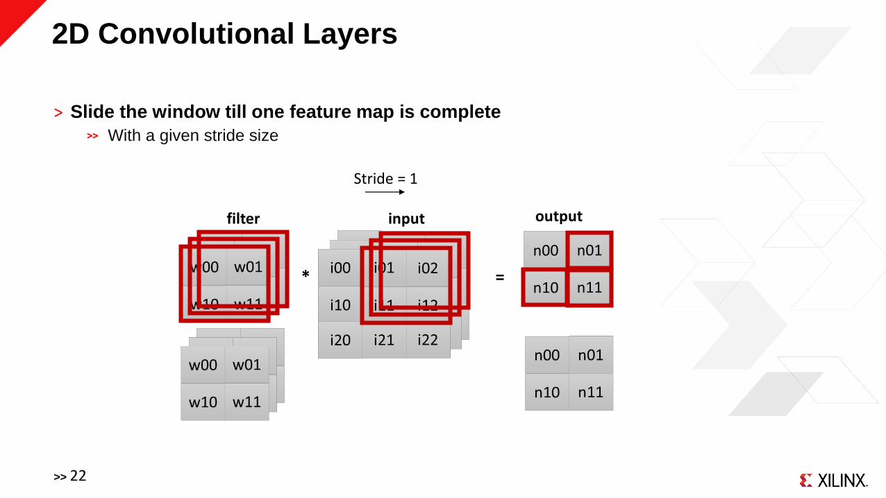
2D Convolutional Layers

˃ Slide the window till one feature map is complete

With a given stride size

w00 w01

w10 w11

filter

i00

i10 i11

input

i02

i12

i20 i21 i22

* =

output

n00 n01

n10 n11

w00 w01

w10 w11

Stride = 1

>> 22

2D Convolutional Layers

˃ Compute next channel

w00 w01

w10 w11

filter

i00 i01

i10 i11

input

i02

i12

i20 i21 i22

* =

output

n00 n01

n10 n11

w00 w01

w10 w11

>> 23

Output channels

2D Convolutional Layers1 input and 1 output channel

˃ Can be lowered to a matrix-matrix multiply using a Toeplitz Matrix

w00 w01

w10 w11

filter

i00 i01

i10 i11

input

i02

i12

i20 i21 i22

* =

output

n00 n01

n10 n11

Convolution

Toeplitz Matrix (“lowered image matrix”)

w00 w01 w10 w11

filterMatrix Vector

x

i00

i01

i11

i10

i01

i02

i11

i12

i10

i11

i20

i21

i11

i12

i21

i22

=

output

n00 n01 n10 n11

<=>

n00 = Act(w00*i00 + w01*i01+w10*i10 + w11*i11)

>> 24

2D Convolutional Layers3 input and 2 output channels

w00 w01

w10 w11

filter

i00 i01

i10 i11

input

i02

i12

i20 i21 i22

* =

output

n00 n01

n10 n11Convolution

filters

Matrix Matrix

output

<=>

w00 w01

w10 w11

…

Input channels

…

Output channel 0,1

Toeplitz Matrix

IN_CH0

IN_CH1

IN_CH2

IN_CH0 IN_CH2In

pu

t ch

ann

el

Output channels

OUT_CH0=xData duplication for taking advantage of linear algebra libraries such as

OpenBLAS, cuBLAS, cuDNN

>> 25

ConvolutionsChallenges

˃ Channel connectivity issue

Every input channel information broadcasts to every output channel

˃ Huge amounts of compute

Dense convolutions account for the majority of the compute

˃ Novel (Non-Dense) Convolutions

Less spatial convolutions (1x1) (SqueezeNet’s FireModules)

Connectivity reduction between in and out channels (Shuffle, Shift layers)

i0

i1

i2

n0

n1

nm-1

…

in-1

#IN

_CH

… #OU

T_C

H

100s to 1000 channels

=> Optimizations

>> 26

MODEL CONV [GOPS] FC [GOPS]ResNet50 7.712 0.004

AlexNet 1.332 0.044

VGG16 30.693 0.247

ConvolutionsChallenges

˃ Parallelization of compute across layers reduces memory bandwidth required for

buffering activations in between layers

˃ Pyramid-shaped data dependency between activations across layers

>> 27 Alwani, M., Chen, H., Ferdman, M. and Milder, P., 2016, October. Fused-layer CNN accelerators. Micro 2016

Pooling Layer

˃ Down-samplers of images

˃ Reduces compute in subsequent layers

˃ May use MAX or AVERAGE

˃ Compute:

Low amount of compute

Potentially replaceable with larger strides in previous convolution

Max pool with 2x2 filters and stride of 2:

i00 i01

i10 i11

input

i02

i12

i20 i21 i22

i03

i13

i23

i30 i31 i32 i33

output

n00 n01

n10 n11

n00 = Max(i00, i01, i10, i11)

>> 28 *Springenberg, J. T., Dosovitskiy, A., Brox, T., & Riedmiller, M. (2014). Striving for Simplicity: The all convolutional net.

Recurrent Layer Types

˃ Contain state for processing sequences

For example needed in speech or optical character recognition

“Apocal???”

˃ Uni-directional or bi-directional

“I ???? You”

˃ More sophisticated types to address the

vanishing gradients problem for learning more

than 5-10 timesteps

GRU (gated recurrent unit)

LSTM (long short term memory)

>> 29

i0

i1

i2

w00

w23

n0

n1

n2

n3

i0

i1

i2

w00

w23

n0

n1

n2

n3

Hopefully the AI Apocalypse won’t happen during my lifetime.

Recurrent LayersChallenges in Additional Data Dependencies

˃ Input sequence

Unlike batch, additional data dependencies between inputs of the same sequence and state

˃ Bi-directional NNs

Full sequence needs to be completed before the next layer

>> 30

Meta-Layers

˃ Residual layers (ResNets *)

Introduced to make larger networks more trainable

Better gradient propagation through skip connections during training

Plus 1x1 convolutions to reduce dimensionality and save compute

˃ Inception layers (GoogleNet**)

Huge variation in spatial features => combining different size convolutions in one layer

Plus 1x1 convolutions to reduce dimensionality and save compute

Later on additional factorization to reduce compute

‒ 3x3 = 1x3 and 3x1

˃ Many more…

˃ Implementation: support for non-linear topologies!

>> 31*He, K., Zhang, X., Ren, S. and Sun, J. "Deep residual learning for image recognition." CVPR’ 2016.** Szegedy, C., Vanhoucke, V., Ioffe, S., Shlens, J. and Wojna, Z. "Rethinking the inception architecture for computer vision." CVPR’ 2016.

+

CNV 3x3, 64, Relu

CNV 3x3, 64, Relu

+

CNV 3x3, 64, Relu

CNV 1x1, 256, Relu

CNV 1x1, 64, Relu

CNV 3x3

CNV 1x1

CNV 5x5

CNV 1x1

CNV 1x1

CNV 3x3CNV 1x1

cc

Elementwise addition

Concatenation

Computation & Memory

Requirements

>> 32

Weights

Compute Activations

Compute and Memory RequirementsArchitecture Neutral, Per Layer

Memory Requirements:𝐴𝑡𝑜𝑡𝑎𝑙 = σ 𝐴𝑖

𝑊𝑡𝑜𝑡𝑎𝑙 = σ 𝑊𝑖

Compute Requirements:𝑂𝑡𝑜𝑡𝑎𝑙 = σ 𝑂𝑖

>> 33

Compute ElementsNumber of Operations : 𝑂𝑖

Layer i

Memory ElementsWeights 𝑊𝑖

Activations 𝐴𝑖

IN, IN_CH: number of inputs and input channelsOUT, OUT_CH: number of outputs and output channelsF_DIM, FM_DIM: filter and feature map dimensions (assumed square)BATCH: batch sizeBITS: bit precision in data typesGATES: number of gates in RNNs: STATES: worst caseSEQ: sequence lengthHID: hidden size (state + output from each state)DIRS: 1 for unidirectional and 2 for bidirectional RNN

Weights

Wi

Inference

Compute

Oi

Activations

Ai

Activations

Ai+1

Inference: Compute & Memory Analysis

>> 34

Fully Connected Layers:𝑊𝑖 ≈ 𝐼𝑁𝑖 * 𝑂𝑈𝑇𝑖* BITS 𝐴𝑖 ≈ BATCH * 𝐼𝑁𝑖* BITS 𝑂𝑖 ≈ 2 ∗ 𝐵𝐴𝑇𝐶𝐻 ∗ 𝐼𝑁𝑖 ∗ 𝑂𝑈𝑇𝑖

Convolutional Layers:𝑊𝑖 ≈ 𝐼𝑁_𝐶𝐻𝑖* 𝑂𝑈𝑇_𝐶𝐻𝑖* 𝐹_𝐷𝐼𝑀𝑖

2 * BITS 𝐴𝑖 ≈ 𝐵𝐴𝑇𝐶𝐻 ∗ 𝐹𝑀_𝐷𝐼𝑀𝑖

2 ∗ 𝐼𝑁_𝐶𝐻𝑖* BITS 𝑂𝑖 ≈ 2 ∗ 𝐵𝐴𝑇𝐶𝐻 ∗ 𝐹𝑀_𝐷𝐼𝑀𝑖

2 ∗ 𝐼𝑁_𝐶𝐻𝑖 ∗ 𝑂𝑈𝑇_𝐶𝐻𝑖* 𝐹_𝐷𝐼𝑀𝑖2

Recurrent Layers:𝑊𝑖 ≈ (𝐹𝑀_𝐷𝐼𝑀𝑖 + 𝐻𝐼𝐷𝑖)* 𝐻𝐼𝐷𝑖 * GATES * DIRS * BITS 𝐴𝑖 ≈ 𝐵𝐴𝑇𝐶𝐻 ∗ 𝐹𝑀_𝐷𝐼𝑀𝑖* DIRS * STATES * SEQ * BITS 𝑂𝑖 ≈ 2 ∗ (𝐹𝑀_𝐷𝐼𝑀𝑖 + 𝐻𝐼𝐷𝑖) * 𝐻𝐼𝐷𝑖 * GATES * DIRS * SEQ

Backpropagation

Weights

Wi

Activations

Ai

Activation

Gradients

AGi+1

Backprop

Compute

Gradients

OBAi

Activation

Gradients

AGi

Backpropagation & Training: Compute & Memory Analysis

Backpropagation for 1 image or 1 sequence and 1 layer𝑊𝐺𝑖 ≈ 𝑊𝑈𝑖 ≈ 𝑊𝑖 2x over inference𝐴𝐺𝑖 ≈ 𝐴𝑖 = inference𝑂𝐵𝑊𝑖 ≈ 𝑂𝐵𝐴𝑖 ≈ 𝑂𝑖 2x over inference(𝑂𝐵𝑊𝑈𝑖 negligible )

Training 1 batch – all layers𝐴𝐵𝑎𝑡𝑐ℎ ≈ 2 ∗ 𝐴𝑊𝐵𝑎𝑡𝑐ℎ ≈ 3 * BATCH * W𝑂𝐵𝑎𝑡𝑐ℎ ≈ 3 * 𝑂𝑖𝑛𝑓𝑒𝑟𝑒𝑛𝑐𝑒

Training overall𝑂𝑂𝑣𝑒𝑟𝑎𝑙𝑙 ≈ 3 * #dataset * #epochs* 𝑂𝑖𝑛𝑓𝑒𝑟𝑒𝑛𝑐𝑒

Weight

Updates

WUi

Weight

Updates

OWUi

>> 35

Forward Pass

Weight

Gradients

WGi

Backprop

Compute

Weights

OBWi

BATCH: size of batch#epochs: number of epochs#datasets: number of inputs in dataset

Inference

Compute

Oi

Inference Compute and MemoryAcross a Spectrum of Neural Networks

Inference (1 input)GOPS

average

Inference (1 input)MBytes

average

Spectrum of Neural Networks

MLP ImageNet Classification CNNsObject

DetectionSemantic

SegmentationOCR

Speech Recognition

*architecture independent**1 image forward *** batch = 1**** int8

GO

PS

and

MB

ytes

resp

ecti

vely

L3 Cache size Processor 1. Inference is hard2. Huge Variation in Compute and Memory Requirements,

even within subgroups3. Models typically don’t fit into cache

>> 36

Training Compute and MemoryAcross a Spectrum of Neural Networks

Training (1 input)MBytes

average

Training (1 input)GOPS

average

Spectrum of Neural Networks

MLP ImageNet Classification CNNsObject

DetectionSemantic

SegmentationOCR

Speech Recognition

*architecture independent**1 image forward and backprop*** batch = 1

1. Training is even harder (just for a 1single image!!)2. Huge Variation in Compute and Memory Requirements,

even within subgroups

>> 37

GO

PS

and

MB

ytes

resp

ecti

vely

Rooflines*

*Williams, S., Waterman, A. and Patterson, D., 2009. Roofline: an insightful visual performance model for multicore architectures. Communications of the ACM>> 38

Theoretical Peak Performance

Memory Bound

Number of Operations per Read/Write Byte in Memory

log axes

Application

Arithmetic IntensityAcross a Spectrum of Neural Networks

˃ Memory requirement for weights, activations are beyond typically available on-chip memory

˃ This yields low arithmetic intensity

For example for inference, assuming weights off-chip and naïve implementation, majority of networks is below 6OPS:Byte

>> 39

* batch = 1** with respect to weights assuming weights are off-chip

Inference

Jouppi, N.P., Young, C., Patil, N., Patterson, D., Agrawal, G., Bajwa, R., Bates, S., Bhatia, S., Boden, N., Borchers, A. and Boyle, R., 2017, June. In-datacenter performance analysis of a tensor processing unit. ISCA’2017

In Summary: CNNs are associated with…

˃ Significant amounts of memory and

computation

˃ Huge variation between topologies and

within them

˃ Fast changing algorithms

˃ Special functions, non-linear topologies

˃ However, incredibly parallel! For convolutions: filter dimensions, feature map dimensions, input & output channels, batches, layers, and even precisions (discussed later)

>> 40

Adopted from Ce Zhang, ETH Zurich, Systems Group Retreat

Architectural Challenges/ Pain Points

>> 41

NN Inference/ Training Accelerator

Input samples

DRAM

Results

Activation Functions/ Pooling…

Weight Buffer

DMA

Input & ActivationBuffering Compute Array

Huge amount of memoryspilling into DRAM

And variations

Weight & activation fetching: bandwidth

throttles performance

Power consumption for embedded

Latency in real-time processing

Partial Sums

Huge amount of compute and variation-Limited scalability with new technology nodes

Requires algorithmic & architectural innovation

Algorithmic Optimization Techniques

>> 42

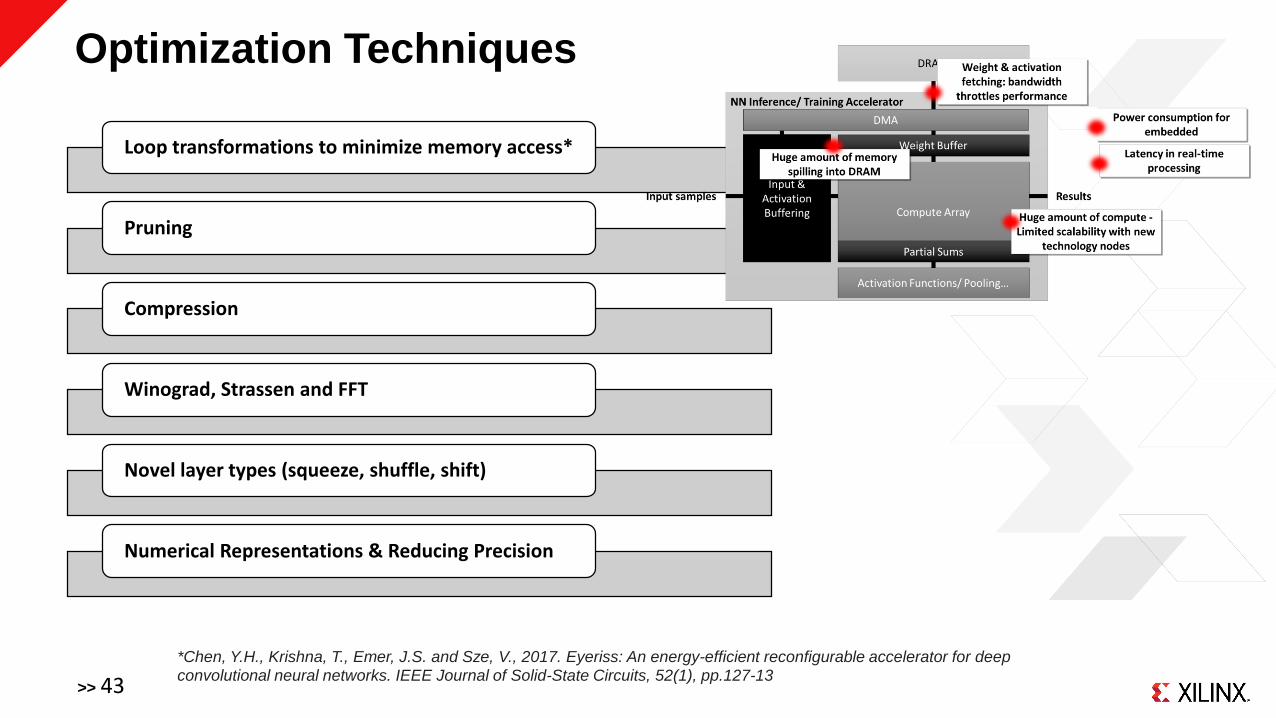
Optimization Techniques

>> 43

Loop transformations to minimize memory access*

Pruning

Compression

Winograd, Strassen and FFT

Novel layer types (squeeze, shuffle, shift)

Numerical Representations & Reducing Precision

*Chen, Y.H., Krishna, T., Emer, J.S. and Sze, V., 2017. Eyeriss: An energy-efficient reconfigurable accelerator for deep convolutional neural networks. IEEE Journal of Solid-State Circuits, 52(1), pp.127-13

Example: Reducing Bit-Precision

˃ Linear reduction in memory footprint

Reduces weight fetching memory bandwidth

NN model may even stay on-chip

˃ Reducing precision shrinks inherent arithmetic cost in both

ASICs and FPGAs

Instantiate 100x more compute within the same fabric and thereby scale performance

Precision Modelsize [MB](ResNet50)

1b 3.2

8b 25.5

32b 102.5

C= size of accumulator * size of weight * size of activation(to appear in ACM TRETS SE on DL, FINN-R)

>> 44

Assumptions: Application can fill device to 90% (fully parallelizable) 710MHz

Reducing Precision provides Performance ScalabilityExample: ResNet50, ResNet152 and TinyYolo

RP reduces model size=> to stay on-chip

Theoretical Peak Performance for a VU13P with different Precision Operations

>> 45

Reducing Precision Inherently Saves Power

Source: Bill Dally (Stanford), Cadence Embedded Neural

Network Summit, February 1, 2017

Target Device ZU7EV ● Ambient temperature: 25 °C ● 12.5% of toggle rate ● 0.5 of Static

Probability ● Power reported for PL accelerated block only

2/2

0.500 0.700 0.900 1.100 1.300 1.500 1.700 1.900 2.100

8

10

12

14

16

18

20

Estimated Power Consumption [W]

Te

st e

rro

r [%

]

LSTM - Test Error vs Power(W)

Bits (W/A)

Pareto Optimal

>> 46Rybalkin, V., Pappalardo, A., Ghaffar, M.M., Gambardella, G., Wehn, N. and Blott, M. "FINN-L: Library Extensions and Design Trade-off Analysis for Variable Precision LSTM Networks on FPGAs."

FPGA:

ASIC:

2/3

3/4

2/42/8

4/4

3/88/8

3/3

4/8

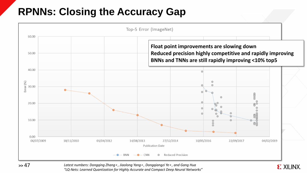
RPNNs: Closing the Accuracy Gap

>> 47

Float point improvements are slowing downReduced precision highly competitive and rapidly improvingBNNs and TNNs are still rapidly improving <10% top5

Latest numbers: Dongqing Zhang∗ , Jiaolong Yang∗ , Dongqiangzi Ye∗ , and Gang Hua “LQ-Nets: Learned Quantization for Highly Accurate and Compact Deep Neural Networks”

0.00

5.00

10.00

15.00

20.00

25.00

30.00

1.0 10.0 100.0 1000.0 10000.0 100000.0 1000000.0 10000000.0 100000000.0 1000000000.0

VA

L. E

RR

OR

(%

)

COMPUTE COST (LUTS + 100*DSPS)

IMAGENET CLASSIFICATION TOP5% VS COMPUTE COST F(LUT,DSP)

1b weights 2b weights 5bit weights 8bit weights FP weights minifloat ResNet-50 Syq

Design Space Trade-Offs

Resnet188b/8bCompute Cost 286Error 10.68%

Resnet502b/8bCompute Cost 127Error 9.86% Reduced Precision can provide better accuracy and lower

hardware cost for specific accuracy targetsIn order to find optimal solutions, solution space needs to be considered and allow for algorithmic freedom

Pareto-optimal solutions

Hardware Architectures and their

Specialization Towards CNN Workloads

Exciting Times in Computer

Architecture Research!

>> 49

Spectrum of New Architectures for Deep Learning

CPUs GPUsSoft DPUs

(FPGA)Hard DPUs

(ASIC)

TPU, Cerebras, Graphcore, Groq, Nervana, Wave Computing, Eyeriss, Movidius, Kalray

IntelAMDARM

AMDNVIDIA

DeePhiTeradeepXDNN

DPU: Deep Learning Processing Unit

>> 50

In-Memory Compute

Using non-volatile resistive memories orstacked DRAM*

*Shafiee, A., Nag, A., Muralimanohar, N., Balasubramonian, R., Strachan, J.P., Hu, M., Williams, R.S. and Srikumar, V., 2016. ISAAC: A convolutional neural network accelerator with in-situ analog arithmetic in crossbars. ACM SIGARCHChi, P., Li, S., Xu, C., Zhang, T., Zhao, J., Liu, Y., Wang, Y. and Xie, Y., 2016, June. Prime: A novel processing-in-memory architecture for neural network computation in reram-based main memory. In ACM SIGARCHChen, Y., Luo, T., Liu, S., Zhang, S., He, L., Wang, J., Li, L., Chen, T., Xu, Z., Sun, N. and Temam, O., 2014, December. Dadiannao: A machine-learning supercomputer. In Proceedings of the 47th Annual IEEE/ACM International Symposium on Microarchitecture (pp. 609-622). IEEE Computer Society.

ISAAC, Tetris,Neurcube

Vector-based SIMD processorsbecoming increasingly customized for Deep Learning

(Tensor Cores, Reduced Precision,…)

Architectural Choices – Macro-Architecture

Soft DPUs(FPGA)

Hard DPUs(ASIC)

Customized macro-architecture

(Synchronous Dataflow)

TPU, Cerebras, Graphcore, Groq, Nervana, Wave Computing, Eyeriss, Movidius, Kalray

MSR Brainwave*

FINN**

DeePhiTeradeepXDNN

>> 51

*Chung, E., Fowers, J., Ovtcharov, K., Papamichael, M., Caulfield, A., Massengill, T., Liu, M., Lo, D., Alkalay, S., Haselman, M. and Abeydeera, M.Serving DNNs in Real Time at Datacenter Scale with Project Brainwave. IEEE Micro, 38(2) https://www.microsoft.com/en-us/research/uploads/prod/2018/06/ISCA18-Brainwave-CameraReady.pdf**Umuroglu, Yaman, Umuroglu, Y., Fraser, N.J., Gambardella, G., Blott, M., Leong, P., Jahre, M. and Vissers, K. “FINN: A framework for fast, scalable binarized neural network inference.” ISFPGA’2017

Matrix of PE

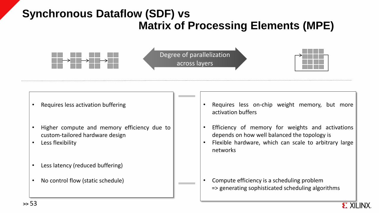
Synchronous Dataflow (SDF) vs Matrix of Processing Elements (MPE)

𝑨𝑻𝒎𝒆𝒎𝒐𝒓𝒚 = 𝑺𝒖𝒎(𝑨𝑻𝒊)

𝑨𝑻𝒊 = 𝒃𝒂𝒕𝒄𝒉 ∗ 𝑭𝑴𝒊𝑫𝑰𝑴 ∗ 𝑪𝑯𝒊 ∗ 𝑲𝒊 + 𝑺𝒊

>> 52

CNVLayer

Weight

WeightsActivationsPing-pong

CNVLayer

Weights

CNVLayer

Weights 𝑾𝑪𝒎𝒆𝒎𝒐𝒓𝒚 = 𝑴𝑨𝑿 𝑾𝒊

𝑨𝑻𝒎𝒆𝒎𝒐𝒓𝒚 =

𝟐 ∗ 𝒃𝒂𝒕𝒄𝒉 ∗ 𝑴𝒂𝒙(𝑭𝑴𝒊𝑫𝑰𝑴 ∗ 𝑭𝑴𝒊𝑫𝑰𝑴 ∗ #𝑪𝑯𝒊)

𝑾𝑪𝒎𝒆𝒎𝒐𝒓𝒚 = 𝑺𝑼𝑴 𝑾𝒊

End points are pure layer-by-layer compute and feed-forward dataflow architecture

Spectrum of Options

MAC, Vector Processor

Lin, X., Yin, S., Tu, F., Liu, L., Li, X. and Wei, S. LCP: a layer clusters paralleling mapping method for accelerating inception and residual networks on FPGA. DAC’2016Alwani, M., Chen, H., Ferdman, M. and Milder, P. Fused-layer CNN accelerators. MICRO 2016.

>> 53

Degree of parallelization across layers

• Requires less activation buffering

• Higher compute and memory efficiency due tocustom-tailored hardware design

• Less flexibility

• Less latency (reduced buffering)

• No control flow (static schedule)

• Requires less on-chip weight memory, but moreactivation buffers

• Efficiency of memory for weights and activationsdepends on how well balanced the topology is

• Flexible hardware, which can scale to arbitrary largenetworks

• Compute efficiency is a scheduling problem=> generating sophisticated scheduling algorithms

Synchronous Dataflow (SDF) vs Matrix of Processing Elements (MPE)

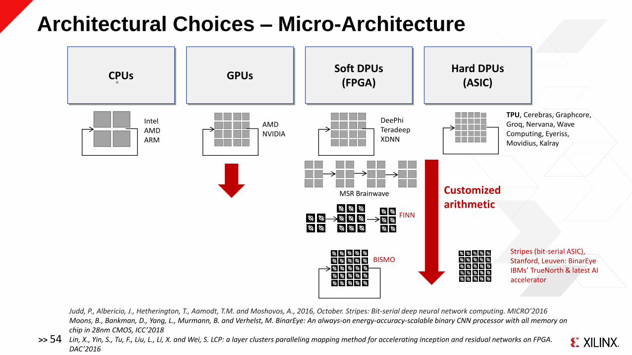
Architectural Choices – Micro-Architecture

CPUs GPUsSoft DPUs

(FPGA)Hard DPUs

(ASIC)

Customized arithmetic

TPU, Cerebras, Graphcore, Groq, Nervana, Wave Computing, Eyeriss, Movidius, Kalray

IntelAMDARM

AMDNVIDIA

MSR Brainwave

FINN

BISMO

DeePhiTeradeepXDNN

>> 54

Stripes (bit-serial ASIC),Stanford, Leuven: BinarEyeIBMs’ TrueNorth & latest AI accelerator

Judd, P., Albericio, J., Hetherington, T., Aamodt, T.M. and Moshovos, A., 2016, October. Stripes: Bit-serial deep neural network computing. MICRO’2016Moons, B., Bankman, D., Yang, L., Murmann, B. and Verhelst, M. BinarEye: An always-on energy-accuracy-scalable binary CNN processor with all memory on chip in 28nm CMOS, ICC’2018Lin, X., Yin, S., Tu, F., Liu, L., Li, X. and Wei, S. LCP: a layer clusters paralleling mapping method for accelerating inception and residual networks on FPGA. DAC’2016

Micro-Architecture:Customized Arithmetic for Specific Numerical Representations

˃ Customizing arithmetic compute allows to maximize

performance at minimal accuracy loss

Flexpoint, Microsoft Floating Point formats, Binary & Ternary, Bfloat16

˃ Which do we support?

Perhaps too risky to support numerous, and too risky to fix on one?

˃ What’s more, non-uniform arithmetic can yield more efficient

hardware implementations for a fixed accuracy*

Run-time programmable precision: Bit-Serial

>> 55*Eunhyeok Park, Junwhan Ahn, and Sungjoo Yoo, “Weighted-Entropy-based Quantization for Deep Neural Networks” CVPR’2017]

Micro-Architecture:Bit-Parallel vs Bit-Serial

˃ Bit-serial can provide run-time programmable precision with a fixed architectureASIC* or FPGA** overlay

˃ FPGA: Flexibility comes at almost no cost and provides equivalent bit-level performance at chip-

level for low precision*

Bit parallel

MAC

A(n)

B(n)

O(m)

Bit serial

MAC

A(n)

B(n)

O(m)

A(n)

Latency vs resource

trade-off

>> 56*Judd, P., Albericio, J., Hetherington, T., Aamodt, T.M. and Moshovos, A., 2016, October. Stripes: Bit-serial deep neural network computing. MICRO’2016**Umuroglu, Rasnayake, Sjalander"BISMO: A Scalable Bit-Serial Matrix Multiplication Overlay for Reconfigurable Computing." FPL’2018 https://arxiv.org/pdf/1806.08862.pdf

Summary

>> 57

Summary

˃ CNNs are increasingly being adopted for new workloads and key to the current

industrial revolution and perhaps the next

˃ Associated with significant challenges

˃ Requires algorithmic and architectural innovation (co-designed)

˃ Emerging: Huge spectrum of algorithms and increasingly diverse & heterogenous

hardware architectures

˃ Clear metrics for comparison needed

Hardware performance always tying back to application performance (accuracy) to allow for algorithmic optimizations

Ideally in form of pareto curves: Accuracy - performance (TOPS/sec) - response time (1 input) -power consumption

>> 58

Exciting Times for our Community:Many New Architectures Evolving - Programmable and Hardened

Application:

Algorithm:

Dataset:

Hardware:

Implementation:

>> 59

• Finding optimal solutions within a multi-dimensional design space combinations trained network topologies on different datasets implemented in different ways on different hardware architectures

Adaptable.

Intelligent.

>> 60

THANK YOU!

Part 1 - Agenda

˃ Neural Networks

˃ Computation & Memory Requirements

˃ Algorithmic Optimization Techniques

˃ Hardware Architectures

>> 61

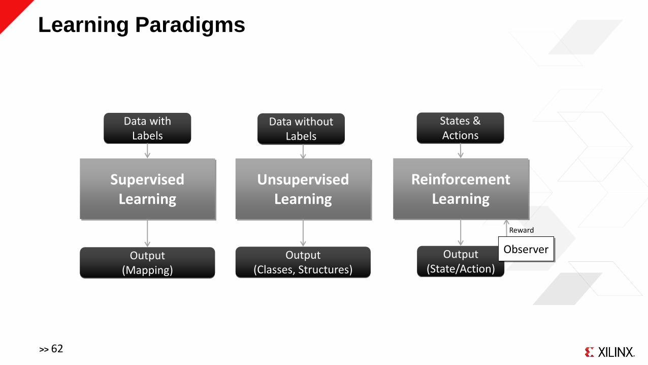
Learning Paradigms

Supervised Learning

Unsupervised Learning

Reinforcement Learning

Data with Labels

Data without Labels

States & Actions

Output(Mapping)

Output(Classes, Structures)

Output(State/Action)

Observer

Reward

>> 62

Batches*

˃ Batch:

Collection of inputs buffered to capitalize on parallelism

˃ Batches in Inference:

Intention is to maximize the compute per loaded weights, helps increase compute efficiency when weight memory bound

‒ Weight_bandwidth = weights*frame-rate/batch

Downside: adverse effects on latency:

‒ Latency >= batch_size * 1/frame rate

˃ Batches in Training:

Batch size (mini-batch or iteration size) also dictates at what intervals weight updates happen)

Larger batch sizes require more memory, and can have potentially adverse effects on accuracy, and smaller batches might have adverse effects on training time

*Caution: Overloaded Terms!

>> 63