Learning Consumer Tastes Through Dynamic Assortments

Citation for published version (APA):Ulu, C., Honhon, D. B. L. P., & Alptekinoglu, A. (2012). Learning Consumer Tastes Through DynamicAssortments. Operations Research, 60(4), 833-849. https://doi.org/10.1287/opre.1120.1067

DOI:10.1287/opre.1120.1067

Document status and date:Published: 01/01/2012

Document Version:Publisher’s PDF, also known as Version of Record (includes final page, issue and volume numbers)

Please check the document version of this publication:

• A submitted manuscript is the version of the article upon submission and before peer-review. There can beimportant differences between the submitted version and the official published version of record. Peopleinterested in the research are advised to contact the author for the final version of the publication, or visit theDOI to the publisher's website.• The final author version and the galley proof are versions of the publication after peer review.• The final published version features the final layout of the paper including the volume, issue and pagenumbers.Link to publication

General rightsCopyright and moral rights for the publications made accessible in the public portal are retained by the authors and/or other copyright ownersand it is a condition of accessing publications that users recognise and abide by the legal requirements associated with these rights.

• Users may download and print one copy of any publication from the public portal for the purpose of private study or research. • You may not further distribute the material or use it for any profit-making activity or commercial gain • You may freely distribute the URL identifying the publication in the public portal.

If the publication is distributed under the terms of Article 25fa of the Dutch Copyright Act, indicated by the “Taverne” license above, pleasefollow below link for the End User Agreement:www.tue.nl/taverne

Take down policyIf you believe that this document breaches copyright please contact us at:openaccess@tue.nlproviding details and we will investigate your claim.

Download date: 16. Feb. 2021

OPERATIONS RESEARCHVol. 60, No. 4, July–August 2012, pp. 833–849ISSN 0030-364X (print) � ISSN 1526-5463 (online) http://dx.doi.org/10.1287/opre.1120.1067

© 2012 INFORMS

Learning Consumer Tastes ThroughDynamic Assortments

Canan UluMcCombs School of Business, The University of Texas at Austin, Austin, Texas 78712,

canan.ulu@mccombs.utexas.edu

Dorothée HonhonSchool of Industrial Engineering, Eindhoven University of Technology, 5612 AZ Eindhoven, The Netherlands,

d.b.l.p.honhon@tue.nl

Aydın AlptekinogluCox School of Business, Southern Methodist University, Dallas, Texas 75275,

aalp@cox.smu.edu

How should a firm modify its product assortment over time when learning about consumer tastes? In this paper, we studydynamic assortment decisions in a horizontally differentiated product category for which consumers’ diverse tastes can berepresented as locations on a Hotelling line. We presume that the firm knows all possible consumer locations, comprising afinite set, but does not know their probability distribution. We model this problem as a discrete-time dynamic program; eachperiod, the firm chooses an assortment and sets prices to maximize the total expected profit over a finite horizon, given itssubjective beliefs over consumer tastes. The consumers then choose a product from the assortment that maximizes their ownutility. The firm observes sales, which provide censored information on consumer tastes, and it updates beliefs in a Bayesianfashion. There is a recurring trade-off between the immediate profits from sales in the current period (exploitation) and theinformational gains to be exploited in all future periods (exploration). We show that one can (partially) order assortmentsbased on their information content and that in any given period the optimal assortment cannot be less informative than themyopically optimal assortment. This result is akin to the well-known “stock more” result in censored newsvendor problemswith the newsvendor learning about demand through sales when lost sales are not observable. We demonstrate that it canbe optimal for the firm to alternate between exploration and exploitation, and even offer assortments that lead to lossesin the current period in order to gain information on consumer tastes. We also develop a Bayesian conjugate model thatreduces the state space of the dynamic program and study value of learning using this conjugate model.

Subject classifications : product assortment; product variety; dynamic programming; Bayesian learning.Area of review : Manufacturing, Service, and Supply Chain Operations.History : Received August 2010; revisions received April 2011, October 2011; accepted February 2012. Published online

in Articles in Advance August 2, 2012.

1. IntroductionConsumers have different tastes, and retailers offering aselection of products to satisfy demand can benefit frominformation on what consumers prefer. Which colors of ashirt should a retailer carry? Should a grocery store carryonly skim and whole milk or should they also carry 1% and2% milk? Information on consumer preferences helps withanticipating consumers’ substitution behavior, forecastingitem-level demand, and ultimately making better productassortment decisions.

There are multiple sources of information a firm canutilize to understand consumer preferences better, such asmarket surveys and (for established products) past salesdata. However, this information may not be readily avail-able or may be too costly for new product categories; forbreakthrough or innovative products the firm may knowlittle about consumer preferences. In this paper, we studyassortment-planning decisions of a retailer who learns

about consumer preferences by experimenting with differentassortments and observing sales. Although a retailer carry-ing established products may not need to experiment withassortments, for products with little information on con-sumer preferences, the firm may want to change its assort-ment dynamically to gather better information.

We consider a horizontally differentiated product cate-gory; products differ with respect to only one attribute forwhich consumers have different first choices provided thatthey cost the same. Products that differ in their fat con-tent, sweetness, spice level, or color are examples. We usea locational choice model à la Hotelling with a discreteset of consumer locations to represent consumer tastes, anda Bayesian framework to model the information-gatheringprocess and the updating of the firm’s beliefs on consumerlocations. The firm knows the set of all possible consumerlocations on the attribute space, starts with a prior distri-bution over these locations, and after observing sales eachperiod, updates this distribution using Bayes’ rule.

833

INFORMS

holds

copyrightto

this

article

and

distrib

uted

this

copy

asa

courtesy

tothe

author(s).

Add

ition

alinform

ation,

includ

ingrig

htsan

dpe

rmission

policies,

isav

ailableat

http://journa

ls.in

form

s.org/.

Ulu, Honhon, and Alptekinoglu: Learning Consumer Tastes Through Dynamic Assortments834 Operations Research 60(4), pp. 833–849, © 2012 INFORMS

This problem exhibits the classic trade-off betweenexploration and exploitation: offering more products inthe assortment allows the firm to gather better informa-tion about consumer tastes because fewer consumers wouldneed to substitute away from their ideal products, however,this may result in lower profits in the short term. On theother hand, offering an assortment that provides the maxi-mum profit in the short term may hinder the information-gathering process and result in less profits in the long run.Beyond this classic trade-off, our demand model allowsus to study the information content of a given assortment.In a Hotelling model, consumers make choices to maximizetheir own utilities, and substitution behavior emerges fromthese optimal choices. Thus, we can study how a givenassortment induces substitution and highlight how assort-ment choice impacts the quality of information a firm canobtain through sales. Because a given assortment may forceconsumers to substitute, there may be some censoring ofconsumer taste information if the firm observes sales. Previ-ous models of learning via dynamic assortments used otherconsumer choice models (e.g., multinomial logit) that donot allow one to analyze the link between product position-ing and substitution behavior explicitly.

First, we study the single-period problem where no learn-ing takes place. The firm determines the optimal assortmentand prices based on a known, discrete distribution of con-sumer tastes. We show that the firm only has to solve forthe optimal market segments, each one corresponding to aproduct, because optimal product locations and prices canbe easily obtained as a function of these market segments.

Second, we consider the finite-horizon problem withlearning under two scenarios to study how censored infor-mation on consumer tastes affect assortment planning:(i) the uncensored information case, in which the firm isable to observe consumer tastes postpurchase, that is, thefirm comes to know the most preferred product for eachconsumer; and (ii) the censored information case, in whichthe firm is only able to observe sales of each product. Thefirm is also uncertain about market size, i.e., how many con-sumers visit the store each period, and we initially assumethat the firm observes the realization of market size at theend of each period. We then extend our analysis to unob-servable market size.

In the uncensored information case, the optimal assort-ment in a given period is the one that maximizes the imme-diate profit; in other words, the firm should adopt a myopicpolicy. In contrast, the optimal assortment in the censoredcase may be such that it is optimal to sacrifice some imme-diate profit in order to gather better information about con-sumer preferences.

The main contribution of this paper is a result thatorders assortments based on their information contentand shows that the optimal assortment under censoredinformation cannot be less informative than the optimalassortment under uncensored information (the myopicallyoptimal assortment). We believe this is a novel result on

the structure of the optimal policy in product assortmentdecisions and is of both theoretical and practical inter-est. Theoretically, it is similar in nature to the “stockmore” result in censored newsvendor problems (see, forexample, Harpaz et al. 1982, Ding et al. 2002, Lu et al.2005). If the newsvendor observes only sales and notdemand, sales observations provide censored informationon demand: depleted inventory only signals that demandmust have been higher than the order quantity. In theseproblems, typically it is optimal to stock more than themyopically optimal order quantity because higher orderquantities provide better information about demand. Ourpaper establishes an analogous result in product assortmentproblems. We discuss the practical relevance of this resultin §4.3; it can decrease the computational effort signifi-cantly and can be used in algorithms that search for a gooddynamic assortment policy. In §6, we show that our keyresult is robust in that a generalized version of our resultholds when we relax our main assumptions.

Research on assortment planning has advanced rapidly inrecent years, particularly on modeling substitution betweenproducts using consumer choice theory from the economicsand marketing literatures. Here, we focus on papers thatconsider dynamic assortments. Kök et al. (2009) providean excellent review of the literature on static assortmentplanning.

A firm might change assortments over time in responseto changes in consumer preferences or in response to fluc-tuating inventory levels. Caldentey and Caro (2010) modelchanging consumer preferences as a stochastic process thata retailer tries to follow and use a stylized representa-tion of the retailer’s assortment as a combination of riskyassets (fashionable items) and risk-free assets (basic items).Their objective is to maximize the long-term value ofdynamically adjusting the menu of products on display.Caro and Martinez-de-Albeniz (2012) propose a satiation-based model of variety-seeking consumers buying frommultiple competing retailers; the model implies that con-sumers spend a higher share of their budget in retailers thatrefresh assortments at a faster pace. Using this novel choicemodel, they derive insights on how often retailers shouldchange assortments in a competitive equilibrium. Bernsteinet al. (2011) study how assortments should be customizeddepending on the profile of remaining inventories.

Some dynamic assortment papers explore how a firmmight learn consumer preferences. Unlike our work, thesepapers either take an aggregate view of consumer choiceor do not explicitly model the attribute space. Caro andGallien (2007) use a finite-horizon multiarmed banditmodel with several plays per stage. Applying a number ofapproximations, they obtain a closed-form dynamic indexpolicy that captures the key exploration versus exploita-tion trade-off, and develop suboptimality bounds. Saureand Zeevi (2011) study a family of assortment-planningproblems in which a general random utility model drivesconsumer choice. They develop dynamic policies that

INFORMS

holds

copyrightto

this

article

and

distrib

uted

this

copy

asa

courtesy

tothe

author(s).

Add

ition

alinform

ation,

includ

ingrig

htsan

dpe

rmission

policies,

isav

ailableat

http://journa

ls.in

form

s.org/.

Ulu, Honhon, and Alptekinoglu: Learning Consumer Tastes Through Dynamic AssortmentsOperations Research 60(4), pp. 833–849, © 2012 INFORMS 835

balance the trade-off between exploration and exploita-tion and prove that these policies satisfy some perfor-mance bounds. Rusmevichientong et al. (2010) constructan algorithm for optimizing dynamic assortments under amultinomial logit choice framework, and explore demandlearning issues. The last two papers take an adaptive learn-ing approach, whereas Caro and Gallien (2007) take aBayesian learning approach, as our paper does. Our resultsapply to any prior distribution and are not limited to a spe-cific conjugate model as in Caro and Gallien (2007).

Our paper contributes to the literature on assortmentplanning in three ways. First, we demonstrate how theinformation on consumer taste that a firm can gatherthrough sales can be censored due to substitution behav-ior and how the firm can control the quality of informationit can obtain through dynamic assortments. This insightis novel mainly because previous models of learning viadynamic assortments do not model the connection betweenassortments and quality of information obtained from salesdirectly. Second, we generate new insights on the structureof optimal assortments and on the exploration-exploitationtrade-off. Whereas previous papers develop good policies,we obtain the optimal policy; our key result comparesthe information content of the optimal assortment and themyopically optimal assortment. Furthermore, although oneintuitively expects the optimal policy to explore first andexploit later, we show that the optimal policy is usuallymore complicated in that it may be optimal to alternatebetween periods of exploration (offering an assortment thatis more informative than the myopically optimal assort-ment) and periods of exploitation (using the myopicallyoptimal assortment). We also study the value of learningby comparing the expected profit obtained under variousassumptions regarding the learning process (i.e., uncen-sored, censored, myopic, and no-learning). We distinguishbetween passive, active, and proactive learning, study theirrelative importance, and show that all three values are highwhen the time horizon is long, and when the firm is uncer-tain and/or has little information about consumer tastes.Third, our paper also contributes to the literature by high-lighting similarities between Bayesian learning models innewsvendor and product assortment problems. In censorednewsvendor models sales observations provide censoredinformation on demand. We analyze a different form ofcensoring, i.e., the censoring of consumer tastes, whichoccurs when the assortment offered by the firm inducesconsumers to purchase a product other than their idealchoice. Using a micromodel of consumer choice behav-ior, we pose a novel censoring problem, which could notbe captured by existing dynamic assortment models in theliterature.

The rest of the paper is organized as follows: wepresent in §2 the locational consumer choice model, andin §3 our results in a single-period setting with no learn-ing. We introduce our multiperiod learning model andits dynamic programming (DP) formulation in §4, and

develop our main results. In §5, we present a numericalstudy, and in §6 we relax some assumptions of our basemodel. We discuss directions for further research in §7.Throughout the paper, we use simple examples to explainour definitions and results. The electronic companion tothis paper is available as part of the online version athttp://dx.doi.org/10.1287/opre.1120.1067.

2. Consumer Choice ModelWe consider consumers making a choice among a set ofhorizontally differentiated products. Let ì ⊆ �, a con-vex set of real numbers, represent the attribute space.Each product is characterized by a single taste attribute,an element of ì, which we refer to as product’s location.We assume that this attribute can be measured on a cardinalscale such as fat content for dairy products.

Consumers choose from n products with locations xi ∈ìand prices pi, i = 11 0 0 0 1 n. The consumer population isheterogeneous in the sense that each consumer has an idealproduct they would purchase if price was not an issue. Thelocation of a consumer’s ideal product, which we refer toas consumer’s location or taste, belongs to a discrete setY = 8y11 y21 0 0 0 1 yN 9, where yj ∈ ì, and N is the numberof consumer types (N < �). We label consumer locationssuch that y1 < y2 < · · ·< yN and at times refer to consumerlocation yj simply as location j .

A consumer located at yj receives utility U4yj1 xi1 pi5=

p−pi −d�yj − xi� from a product located at xi and pricedat pi. Here, p is the consumer’s willingness-to-pay for hisideal product, which we refer to as the reservation price,and d is a disutility that the consumer incurs per unit ofdistance between his location and the product’s location,which we refer to as the transportation cost. We assumethat the reservation price and transportation cost are thesame for all consumers (we relax the former assumptionin §6).

Consumers have an outside option with a fixed utilitythat we set to zero without loss of generality. Each con-sumer buys the product that gives him the highest utility,or opts out and obtains zero utility from not buying anyof the n products. That is, a consumer located at yj buysproduct i if i = arg maxk∈81121 0001 n98p−pk −d�yj − xk�9, andp¾ pi + d�yj − xi�. If such a product does not exist (all nproducts result in negative utility), the consumer choosesthe outside option.

This locational consumer choice model dates back toLancaster (1966), who has extended the work of Hotelling(1929) on spatial competition. Lancaster’s model involvesa uniform density of consumers in a continuous attributespace. Gaur and Honhon (2006) and Alptekinoglu andCorbett (2010) use the model with a continuous andnonuniform distribution of consumer tastes in operationsmanagement settings. In contrast, we take a finitely count-able set of discrete points in the attribute space as consumerlocations, which are known to the firm, and assume a gen-eral discrete probability distribution (possibly nonuniform)over it.

INFORMS

holds

copyrightto

this

article

and

distrib

uted

this

copy

asa

courtesy

tothe

author(s).

Add

ition

alinform

ation,

includ

ingrig

htsan

dpe

rmission

policies,

isav

ailableat

http://journa

ls.in

form

s.org/.

Ulu, Honhon, and Alptekinoglu: Learning Consumer Tastes Through Dynamic Assortments836 Operations Research 60(4), pp. 833–849, © 2012 INFORMS

3. Single-Period ProblemIn this section, we study a firm that makes product loca-tion and pricing decisions to maximize expected profit in asingle period, knowing the probability distribution of con-sumer tastes.

Suppose the firm offers n products with locations x ≡

4x11 x21 0 0 0 1 xn5 with xi ∈ ì, and prices p ≡ 4p11 p210 0 0 1 pn5. Let the products be numbered such that x1 < x2 <· · · < xn. We define the market segment captured by prod-uct i ∈ 81121 0 0 0 1 n9, denoted by ai ⊆ ì, as a subset ofthe attribute space such that all consumers located withinai choose to purchase product i, over all the other prod-ucts and the outside option, in accordance with the choicebehavior described in §2. Clearly, ai depend on x andp through consumer choice; we study this dependence inLemma 1.

Let �j be the probability that a randomly chosen con-sumer is at location yj . A random number of consumers, m,visit the firm’s store during the period (we use tilde todistinguish random variables from their realized values).We refer to m as the market size, a discrete random vari-able independent of consumer locations, and assume thatthe firm knows its expected value, �≡ Ɛ6m7. One can alsointerpret �j as the proportion of consumers in the popula-tion who are located at yj , and m as the size of a randomlyselected sample from this population. Thus, the vector ofprobabilities È ≡ 4�11 �21 0 0 0 1 �N 5 with

∑Nj=1 �j = 1 spec-

ifies the distribution of consumer locations, and the firmknows these probabilities.

The timing of events within the period is as follows.First, the firm determines the locations x and prices p ofproducts to offer, based on the expected market size � andthe vector of probabilities È. Subsequently, m consumersvisit the store and make purchase decisions based on xand p as described in §2. The firm is not able to price-discriminate based on consumer tastes because it is not ableto observe them at the time of product location and pricingdecisions.

The demand for product i, Di depends on its mar-ket segment, and it is a random variable with expectedvalue ƐÈ6Di4ai4x1p557 = �

∑

j2 yj∈ai�j . A consumer pur-

chases product i only if his location falls in ai; this happenswith probability

∑

j2 yj∈ai�j . We emphasize that the expec-

tation above depends on È by writing ƐÈ6 · 7.The firm incurs a fixed cost, f > 0, for each product

offered, and a variable cost of production, c > 0, per unit ofproduct sold. Sales equal demand because we assume awaysupply-demand mismatches. We assume throughout that themarket is profitable, c < p, otherwise the firm would preferto offer no products. We express the firm’s expected profitas follows:

r4x1p1È5= −fn+

n∑

i=1

4pi − c5ƐÈ6Di4ai4x1p5570 (1)

We first study how product assortment decisions andmarket segments that result from consumer choice behaviorare related.

Lemma 1. Optimal product locations and prices, x and p,must satisfy the following properties:

(a) Market segments that result from x and p are mutu-ally disjoint and closed intervals in ì, and their bound-ary points belong to the set of consumer locations, i.e.,ai = 6xi1 xi7 ⊆ ì with xi1 xi ∈ Y such that xi ¶ xi fori = 11 0 0 0 1 n and xi < xi+1 for i = 11 0 0 0 1 n− 1.

(b) Products are located and priced such that consumersat the boundary points of market segments obtain zero netutility from purchase, i.e., xi = 4xi + xi5/2 and pi = p −

d4xi − xi5/2, for i = 11 0 0 0 1 n.

The most important implication of Lemma 1 is that thesingle-period problem reduces to that of setting bound-ary points for market segments. That is, optimizing prod-uct locations x and prices p is equivalent to optimizinga ≡ 4a11 0 0 0 1 an5= 46x11 x171 0 0 0 1 6xn1 xn75, which we referto as the assortment. Moreover, finding the optimal assort-ment is a matter of choosing boundary points for n dis-joint intervals from the set of consumer locations Y . Oncethe firm chooses boundary points of market segments opti-mally, optimal product locations and optimal prices are alsoeffectively set.

The number of products to offer, n, is itself a decision,and it is possible that the firm may not want to cover theentire market. We say that consumer location yj is coveredif there exists a product i such that yj ∈ ai; otherwise, wesay it is not covered. Because the optimal market segmentsare disjoint, each consumer location is covered by at mostone product.

Letting A be the set of all possible assortments that sat-isfy the properties shown in Lemma 1, we rewrite the firm’ssingle-period assortment-planning problem as follows:

maxa∈A

r4a1È5= −fn+

n∑

i=1

4pi4ai5− c5ƐÈ6Di4ai571

where pi4ai5= p−d44xi − xi5/25 and

ƐÈ6Di4ai57=�∑

j2 yj∈ai

�j 0

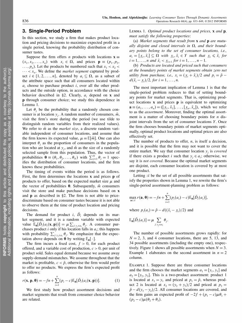
The number of possible assortments grows rapidly: forN = 2, 3, and 4 consumer locations, there are 5, 13, and34 possible assortments (including the empty one), respec-tively. Figure 1 shows all possible assortments when N = 3.Example 1 elaborates on the second assortment in n = 2column.

Example 1. Suppose there are three consumer locationsand the firm chooses the market segments a1 = 6y11 y17 anda2 = 6y21 y37. This is a two-product assortment: product 1is located at x1 = y1 and priced at p1 = p, whereas prod-uct 2 is located at x2 = 4y2 + y35/2 and priced at p2 =

p−d4y3 − y25/2. All consumer locations are covered, andthe firm gains an expected profit of −2f + 4p1 − c5��1 +

4p2 − c5�4�2 + �35.

INFORMS

holds

copyrightto

this

article

and

distrib

uted

this

copy

asa

courtesy

tothe

author(s).

Add

ition

alinform

ation,

includ

ingrig

htsan

dpe

rmission

policies,

isav

ailableat

http://journa

ls.in

form

s.org/.

Ulu, Honhon, and Alptekinoglu: Learning Consumer Tastes Through Dynamic AssortmentsOperations Research 60(4), pp. 833–849, © 2012 INFORMS 837

Figure 1. All possible assortments for N = 3 (×’s denote product locations; triangles denote market segments).

y1 y2 y3

n = 0 n = 1 n = 2 n = 3

Solving the above problem for the optimal single-periodassortment is equivalent to solving a shortest-path problemof complexity O4N 25; see Alptekinoglu et al. (2012) forfurther details. Chen et al. (1998) and Alptekinoglu andCorbett (2010) use a similar solution method. Unlike ourmodel, both papers use a continuous attribute space forproducts and consumers, and neither paper accounts for thepossibility of not covering some portions of the market.

4. Multiperiod Model with LearningFirms do not necessarily know the distribution of consumertastes for many products, especially for new ones. A firmthat is highly uncertain about the distribution of consumertastes can use product assortments as information-gatheringinstruments. Such an undertaking must optimally trade offinformation gathered on consumer tastes by observing salesof an assortment (which can be exploited in the long run)with the profits earned in the short term. We study thistrade-off, commonly known as the exploration-exploitationtrade-off.

In particular, we consider a firm that makes product loca-tion and pricing decisions every period to maximize totaldiscounted expected profits over a finite planning horizon.The timing of events is as follows. At the start of eachperiod, the firm determines the product locations x andprices p, paying a fixed cost f for each product offered.In practice, f may correspond to shelf space and advertis-ing related costs recurring every period for each product.Subsequently, consumers visit the firm’s store and makepurchase decisions in accordance with §2. We assume thatthe market size is uncertain, but that the firm knows itsdistribution; we let P4m = m5 be the probability that themarket size in any given period is m for m = 0111 0 0 0 1Mand M ¶ �. The firm is also uncertain about consumertastes, in the sense that although the firm knows the (finite)set of possible consumer locations, it does not know therelative proportions of these locations in the consumer pop-ulation (we discuss the possibility of unknown consumerlocations in §6). We represent this uncertainty by a contin-uous random variable È≡ 4�11 �21 0 0 0 1 �N 5 with �j denotingthe probability that a randomly chosen consumer is at loca-tion yj ∈ Y , or, equivalently, the unknown proportion ofconsumers from location yj ∈ Y in the consumer population

(in the latter interpretation, each consumer from the popu-lation is equally likely to visit the store in a given period).Hence, there are two independent sources of uncertainty:the consumer taste distribution È and the market size m.In each period the firm observes how many consumersvisit the store (including those who choose not to makea purchase) and the purchase decision of each consumer.At the end of the period, the firm uses this information toupdate its beliefs about the distribution of consumer tastesusing Bayes’ rule. The updated beliefs are then used inthe next period to decide on the product assortment. As inthe single-period model, the firm cannot price-discriminatebased on consumer tastes because it is not able to observethem at the time of product assortment decisions. More-over, we assume that the market size is independent of thechosen assortment, which allows us to focus on the qualityof information obtained through different assortments.

The assumption of observable market size is realistic foronline sales because most companies now have the technol-ogy to count the total number of consumers who visit theirsites. Even brick-and-mortar stores have a very good under-standing, if not a reasonably accurate estimate, of theirstore traffic (at store entrances one frequently sees greeterswith counters in their hands). Nowadays, some retailerseven make use of digital imaging to count and track thebehavior of customers in various aisles of the store (seeOlivares et al. 2011). In §6 we relax the assumption that themarket size is observable. We present the case of observ-able market size first in order to study the learning of con-sumer tastes in isolation, free of market-size effects. In theunobservable case, the market-size uncertainty also affectsthe inference on consumer tastes, further complicating thelearning process.

We first specify how the firm updates its beliefs on con-sumer tastes in a generic period.

4.1. Updating Beliefs on Consumer Tastes

Suppose the firm initially has a prior distribution �4È5on È. We distinguish two cases: (i) uncensored informa-tion and (ii) censored information. The uncensored infor-mation case is a theoretical benchmark in which the firmis able to observe all consumer locations. The censoredinformation case is a realistic setting in which the firm

INFORMS

holds

copyrightto

this

article

and

distrib

uted

this

copy

asa

courtesy

tothe

author(s).

Add

ition

alinform

ation,

includ

ingrig

htsan

dpe

rmission

policies,

isav

ailableat

http://journa

ls.in

form

s.org/.

Ulu, Honhon, and Alptekinoglu: Learning Consumer Tastes Through Dynamic Assortments838 Operations Research 60(4), pp. 833–849, © 2012 INFORMS

observes sales data only (no consumer locations). Our pri-mary purpose in introducing the uncensored informationcase is to understand the effect of censoring, which resultsfrom consumers’ substitution behavior, on dynamic assort-ment decisions.

Uncensored information. Suppose the firm observes mar-ket size and consumer tastes at the end of each period, thatis, the firm is able to observe the location of each con-sumer who comes to the store, including those who do notpurchase a product. Let Tj be the number of consumers atlocation j and let T = 4T11 0 0 0 1 TN 5 be the consumer tastesvector. We use superscript u to denote the uncensored infor-mation case. Given È and a market-size realization m, theconditional distribution of consumer tastes (or the likeli-hood function), Lu4T �È1m5, is a multinomial distribution

Lu4T �È1m5=m!

T1!T2! · · ·TN !�T11 · · ·�

TNN (2)

defined for all T such that∑N

j=1 Tj = m. If the firmstarts with a prior � and observes tastes T = 4T11 0 0 0 1 TN 5,the uncensored posterior distribution is çu4È3�1T1m5 =

Lu4T �È1m5�4È5/f u4T3�1m5. Here, çu is the Bayesianupdating operator with uncensored taste information andf u4T3�1m5 =

∫

ÈLu4T �È1m5�4È5dÈ is the probability

mass function for consumer tastes conditional on m.Censored information. In this case, the firm observes

sales information for the assortment it offers in additionto the market size at the end of each period. Because theassortment can be such that consumers from multiple loca-tions buy the same product, the taste information may becensored. Let D = 4D11 0 0 0 1Dn5 denote the observed salesvector for assortment a with n ¶ N products. We use thesuperscript c to denote the censored information case. Theconditional distribution of sales, Lc4D �È1m1a5, dependson the assortment a, and is given by

Lc4D �È1m1a5=m!

D1! · · ·Dn!4m−D05!

·

n∏

i=1

(

∑

j2 yj∈ai

�j

)Di(

∑

j2 yjy∪ni=1ai

�j

)m−D0

1 (3)

where D0 =∑n

i=1 Di ¶m. Each of the n terms in the mul-tiplication corresponds to a group of locations that arecovered by one product in assortment a, and the last termcorresponds to all the remaining locations (if any) that arenot covered.

Example 2. Suppose there are three consumer locations.If the firm offers a product that covers location 1only, a = 46y11 y175, the conditional distribution of salesD1 is Lc4D1 �È, m1 46y11 y1755 = 4m!/4D1!4m−D15!55 ·

�D11 4�2 + �35

m−D1 . On the other hand, if the firm chooses tooffer one product that covers both locations 1 and 2, a =

46y11 y275, the conditional distribution of sales is Lc4D1 �È,m1 46y11 y2755= 4m!/4D1!4m−D15!554�1 + �25

D1�m−D13 .

If the firm starts with prior �, chooses assortment a,then observes sales D and market size m, the cen-sored posterior distribution on È is çc4È3�1D1m1a5 =

Lc4D �È1m1a5�4È5/f c4D3�1m1a5. Here, çc is theBayesian updating operator with censored taste informa-tion and f c4D3�1m1a5 =

∫

ÈLc4D �È1m1a5�4È5dÈ is the

probability mass function for D under a conditional on m.The analysis in the following sections is general as it

holds for any continuous prior �. We discuss conjugatemodels for both the uncensored and censored informationcases in §4.4.

4.2. Dynamic Programming Formulation

As in the single-period problem, the firm can decide on theassortment a ∈ A in each period as opposed to x and p.Given the assortment, x and p are as in Lemma 1 in §3.

In the uncensored information case, we write the optimalvalue function with t periods remaining, vut 4�5, as a DPrecursion. With zero periods remaining, the optimal valuefunction is vu04�5= 0. For earlier periods, we take the opti-mal value function to be

vut 4�5= maxa∈A

r4a1�5+ �Ɛ�6vut−14ç

u4�1 T1 m5571 (4)

where � is the discount factor (0 ¶ � ¶ 1). The totalprofit the firm receives from assortment a is the sum ofimmediate profit, r4a1�5, and the expected profit-to-go,Ɛ�6v

ut−14ç

u4�1 T1 m557. Here, and in the remaining sec-tions, we emphasize that expectations depend on our statevariable � by writing Ɛ�6·7. As in the single-period prob-lem, we write the immediate profit from assortment aas r4a1�5 = −fn +

∑ni=14pi4ai5 − c5Ɛ�6Di4ai57, where

Ɛ�6Di4ai57 = �∑

j2 yj∈aiƐ�6�j 7 is the expected demand for

product i and Ɛ�6�j 7 =∫

�j�4È5dÈ is the expected valueof �j under prior �.

The expected profit-to-go in (4) takes into account theuncertainty about consumer tastes and the market size to beobserved next period and can be written more explicitly as

Ɛ�6vut−14ç

u4�1 T1 m557

=∑

m

∑

T

vut−14çu4�1T1m55f u4T3�1m5P4m=m50

Because our DP state variable is a probability distribu-tion, we frequently suppress the domain of the distribu-tion and write the posterior as çu4�1T1m5 when we wantto consider this distribution as a function of the prior �,observed taste vector T, and market size m.

We write an analogous DP recursion for the optimalvalue function in the censored information case when thefirm does not observe consumer tastes directly but has toinfer them through sales in each period. With zero periodsremaining, we take vc04�5= 0. For earlier periods, we take

vct 4�5= maxa∈A

{

r4a1�5+ �Ɛ�6vct−14ç

c4�1 D1 m1a557}

1 (5)

INFORMS

holds

copyrightto

this

article

and

distrib

uted

this

copy

asa

courtesy

tothe

author(s).

Add

ition

alinform

ation,

includ

ingrig

htsan

dpe

rmission

policies,

isav

ailableat

http://journa

ls.in

form

s.org/.

Ulu, Honhon, and Alptekinoglu: Learning Consumer Tastes Through Dynamic AssortmentsOperations Research 60(4), pp. 833–849, © 2012 INFORMS 839

where Ɛ�6vct−14ç

c4�1 D1 m1a557 =∑

m

∑

D vct−14ç

c4�1D1m1a55f c4D3�1m1a5P4m=m5.

Note that in (4), the assortment a affects only the imme-diate profit, r4a1�5. Thus, the optimal assortment in theuncensored information case can be solved for myopicallyusing the shortest-path formulation in Alptekinoglu et al.(2012). This is not the case when the consumer taste infor-mation is censored; the assortments chosen over multipleperiods affect both immediate profits and expected profits-to-go. In the censored information case, the myopicallyoptimal assortment does not necessarily result in the highestprofit-to-go; the firm needs to trade off immediate profitswith informational gains (learning benefits) when choosingthe optimal assortment.

4.3. Comparing Optimal Assortments inCensored and UncensoredInformation Cases

We first show that the value functions in (4) and (5) areconvex in the firm’s beliefs, �, each period. This propertyhelps us study how the optimal assortments compare incensored and uncensored information cases.

Proposition 1. Given any two priors �1 and �2, let��4È5 = ��14È5 + 41 − �5�24È5 for some � ∈ 60117.Then, vct 4��5 ¶ �vct 4�15 + 41 − �5vct 4�25 and vut 4��5 ¶�vut 4�15 + 41 − �5vut 4�25, that is, the value functions areconvex in �.

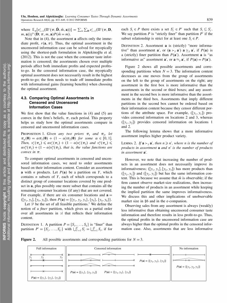
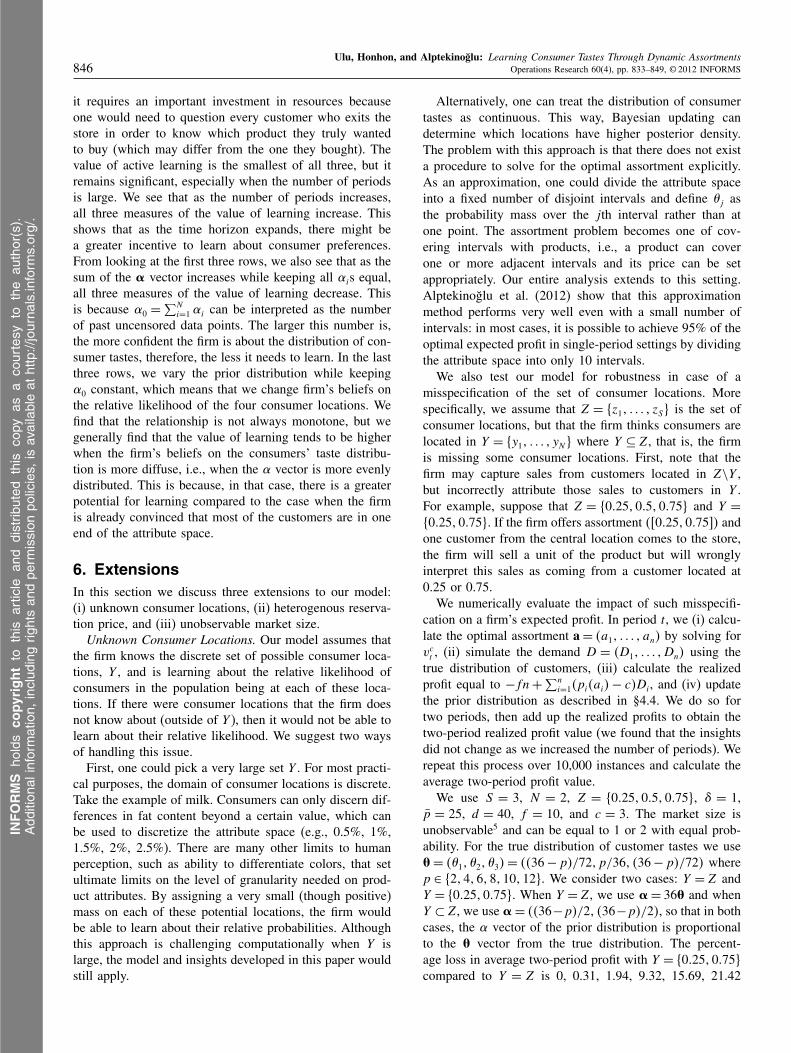
To compare optimal assortments in censored and uncen-sored information cases, we need to order assortmentsbased on their information content. Consider an assortmenta with n products. Let P4a5 be a partition on Y , whichcontains n subsets of Y , each of which corresponds to adistinct group of consumer locations covered by one prod-uct in a, plus possibly one more subset that contains all theremaining consumer locations (if any) that are not covered.For example, if there are six consumer locations and a =

46y11 y371 6y51 y575, then P4a5= 88y11 y21 y391 8y591 8y41 y699.Let P be the set of all feasible partitions.1 We define the

notion of a finer partition, which gives us a partial orderover all assortments in A that reflects their informationcontent.

Definition 1. A partition P = 8S11 0 0 0 1 Sk9 is “finer” thanpartition P ′ = 8S ′

11 0 0 0 1 S′k′9 with

⋃k′

i′=1 S′i′ =

⋃ki=1 Si, if for

Figure 2. All possible assortments and corresponding partitions for N = 3.

y1 y2 y3

No informationCensored informationFull information

P(a) = {{y1}, {y2}, {y3}}

P(a) = {{y1, y2}, {y3}}

P(a) = {{y1, y2, y3}}

P(a) = {{y1}, {y2, y3}}

P(a) = {{y1, y3}, {y2}}

each Si ∈ P there exists a set S ′i′ ∈ P ′ such that Si ⊆ S ′

i′ .We say partition P is “strictly finer” than partition P ′ if thesubset relationship is strict for at least one Si ∈ P .

Definition 2. Assortment a is (strictly) “more informa-tive” than assortment a′, or (a �I a′) a �I a′, if P4a5 isa (strictly) finer partition than P4a′5. Assortment a is “asinformative as” assortment a′, or a ≈I a′, if P4a5= P4a′5.

Figure 2 shows all possible assortments and corre-sponding partitions when N = 3. The information contentdecreases as one moves from the group of assortmentson the left to the group of assortments on the right; anyassortment in the first box is more informative than theassortments in the second or third boxes; and any assort-ment in the second box is more informative than the assort-ments in the third box. Assortments that imply differentpartitions in the second box cannot be ordered based ontheir information content because they censor different por-tions of the attribute space. For example, 46y11 y175 pro-vides censored information on locations 2 and 3, whereas46y11 y275 provides censored information on locations 1and 2.

The following lemma shows that a more informativeassortment implies higher product variety.

Lemma 2. If a �I a′, then n¾ n′, where n is the number ofproducts in assortment a and n′ is the number of productsin assortment a′.

However, we note that increasing the number of prod-ucts in an assortment does not necessarily improve itsinformativeness; 46y11 y171 6y21 y375 has more products than46y11 y175 and 46y21 y375 but has the same information con-tent. This is because we assume that m is observable; if thefirm cannot observe market-size realizations, then increas-ing the number of products in an assortment while keepingthe implied partition the same improves informativeness.We discuss this and other implications of unobservablemarket size in §6 and in the e-companion.

Observing sales from any assortment is always (weakly)less informative than obtaining uncensored consumer tasteinformation and therefore results in less profit-to-go. Thus,the optimal profits in the uncensored information case arealways higher than the optimal profits in the censored infor-mation case. Also, assortments that are less informative

INFORMS

holds

copyrightto

this

article

and

distrib

uted

this

copy

asa

courtesy

tothe

author(s).

Add

ition

alinform

ation,

includ

ingrig

htsan

dpe

rmission

policies,

isav

ailableat

http://journa

ls.in

form

s.org/.

Ulu, Honhon, and Alptekinoglu: Learning Consumer Tastes Through Dynamic Assortments840 Operations Research 60(4), pp. 833–849, © 2012 INFORMS

result in lower profits-to-go. To prove these results, we firstprove a lemma on optimal profit-to-go functions.

Lemma 3. For any convex function u4�5 and assortmentsa �I a′, we have

Ɛ�6u4çu4�1 T1 m557¾ Ɛ�6u4ç

c4�1 D1 m1a557

¾ Ɛ�6u4çc4�1 D1 m1a′5570

Using this lemma, we show that the optimal profits with-out censoring are higher than optimal profits with censoringand that it cannot be optimal to select a less informativeassortment in the censored information case than the opti-mal assortment in the uncensored information case.

Theorem 1. For all t, we have vut 4�5 ¾ vct 4�5. More-over, if the optimal assortment in the uncensored infor-mation case when there are t periods to go is a∗,then for any assortment a such that a∗ �I a, wehave vct 4�3a∗5 ¾ vct 4�3a51 where vct 4�3a5 = r4a1�5 +

�Ɛ�6vct−14ç

c4�1 D1 m1a557. Therefore, the value functionfor the uncensored information case is always higher, andthe optimal assortment in the censored information casecannot be less informative than the optimal assortment inthe uncensored information case (i.e., the myopically opti-mal assortment).

Proof. We first show that vut 4�5 ¾ vct 4�5. The prooffollows by induction. When there is one period to go,vu14�5 = vc14�5. Now, assume vut−14�5 ¾ vct−14�5. Forany given prior � and assortment a, Proposition 1 andLemma 3 imply the first inequality below, and the inductionhypothesis implies the second: Ɛ�6v

ut−14ç

u4�1 T1 m557 ¾Ɛ�6v

ut−14ç

c4�1 D1 m1a557 ¾ Ɛ�6vct−14ç

c4�1 D1 m1a557.This then implies that vut 4�5 ¾ vct 4�5. Now, assume thata∗ is the optimal assortment in the uncensored informationmodel: a∗ = arg max r4a1�5 + �Ɛ�6v

ut−14ç

u4�1 T1 m557.For any assortment a such that a∗ �I a, we have r4a∗1�5¾r4a1�5, because the optimal policy in the uncensoredinformation case is myopic. Using Proposition 1 andLemma 3, we also have Ɛ�6v

ct−14ç

c4�1 D1 m1a∗557 ¾Ɛ�6v

ct−14ç

c4�1 D1 m1a557. Therefore, for any a such thata∗ �I a, we have vct 4�3a∗5¾ vct 4�3a5. �

This result is analogous to the “stock more” resultderived from censored newsvendor problems, in which the

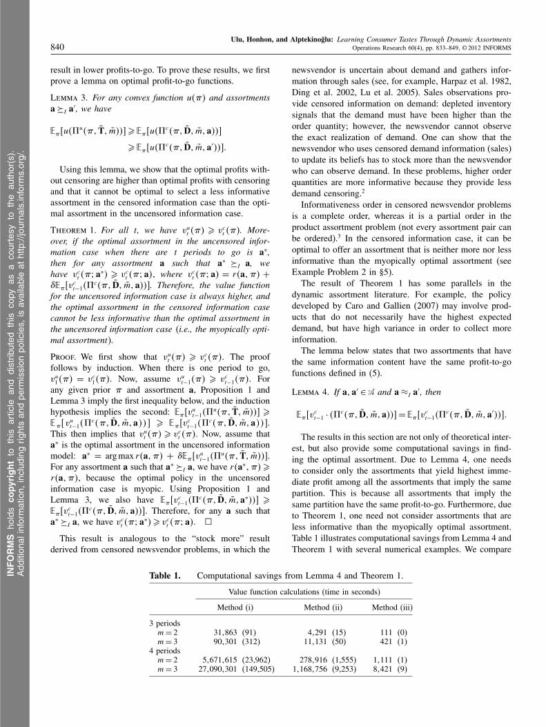
Table 1. Computational savings from Lemma 4 and Theorem 1.

Value function calculations (time in seconds)

Method (i) Method (ii) Method (iii)

3 periodsm= 2 311863 (91) 41291 (15) 111 (0)m= 3 901301 (312) 111131 (50) 421 (1)

4 periodsm= 2 516711615 (23,962) 2781916 (1,555) 11111 (1)m= 3 2710901301 (149,505) 111681756 (9,253) 81421 (9)

newsvendor is uncertain about demand and gathers infor-mation through sales (see, for example, Harpaz et al. 1982,Ding et al. 2002, Lu et al. 2005). Sales observations pro-vide censored information on demand: depleted inventorysignals that the demand must have been higher than theorder quantity; however, the newsvendor cannot observethe exact realization of demand. One can show that thenewsvendor who uses censored demand information (sales)to update its beliefs has to stock more than the newsvendorwho can observe demand. In these problems, higher orderquantities are more informative because they provide lessdemand censoring.2

Informativeness order in censored newsvendor problemsis a complete order, whereas it is a partial order in theproduct assortment problem (not every assortment pair canbe ordered).3 In the censored information case, it can beoptimal to offer an assortment that is neither more nor lessinformative than the myopically optimal assortment (seeExample Problem 2 in §5).

The result of Theorem 1 has some parallels in thedynamic assortment literature. For example, the policydeveloped by Caro and Gallien (2007) may involve prod-ucts that do not necessarily have the highest expecteddemand, but have high variance in order to collect moreinformation.

The lemma below states that two assortments that havethe same information content have the same profit-to-gofunctions defined in (5).

Lemma 4. If a1a′ ∈A and a ≈I a′, then

Ɛ�6vct−1 · 4çc4�1 D1 m1a557= Ɛ�6v

ct−14ç

c4�1 D1 m1a′5570

The results in this section are not only of theoretical inter-est, but also provide some computational savings in find-ing the optimal assortment. Due to Lemma 4, one needsto consider only the assortments that yield highest imme-diate profit among all the assortments that imply the samepartition. This is because all assortments that imply thesame partition have the same profit-to-go. Furthermore, dueto Theorem 1, one need not consider assortments that areless informative than the myopically optimal assortment.Table 1 illustrates computational savings from Lemma 4 andTheorem 1 with several numerical examples. We compare

INFORMS

holds

copyrightto

this

article

and

distrib

uted

this

copy

asa

courtesy

tothe

author(s).

Add

ition

alinform

ation,

includ

ingrig

htsan

dpe

rmission

policies,

isav

ailableat

http://journa

ls.in

form

s.org/.

Ulu, Honhon, and Alptekinoglu: Learning Consumer Tastes Through Dynamic AssortmentsOperations Research 60(4), pp. 833–849, © 2012 INFORMS 841

the number of value function calculations and computationtime when the value functions are computed in three differ-ent ways: (i) by comparing the sum of immediate rewardand profit-to-go function for every possible assortment (i.e.,complete enumeration), (ii) by comparing only the assort-ments that yield the highest immediate profits for each par-tition (i.e., using Lemma 4), (iii) by comparing only theassortments that yield the highest immediate profits for eachpartition and that are not less informative than the myopi-cally optimal assortment (i.e., using Lemma 4 and Theo-rem 1). We use the following parameters: � has a Dirichletdistribution with Á = 41, 1, 1, 1), Y = 8002, 0.4, 0.6, 0089,� = 1, p = 20, d = 20, c = 3, and f = 1 (see §4.4 for thedetails of how Bayesian updating works under a Dirich-let prior). We vary m ∈ 82139 and the number of periodsin 83149.

We see that although Lemma 4 and Theorem 1 do notchange the theoretical complexity of the search for theoptimal solution, in practice they may lead to significanttime savings. This is especially true when m is large andthere are many time periods, which is likely to be the casein practice (we found that the other parameters had littleimpact on the magnitude of the computational savings).

4.4. Conjugate Models

The analysis so far holds for any prior distribution, �. Here,we study conjugate learning models where posteriors arein the same family of distributions as priors. This propertymakes Bayesian updating easier and allows us to reduce thestate space of our DP model. Also, we use these conjugatemodels in our numerical study in §5.

Uncensored Information. The likelihood function in theuncensored information case is given in (2) and is amultinomial distribution. The conjugate prior for a multi-nomial distribution is the Dirichlet distribution. Its proba-bility density function with parameters Á = 4�11 0 0 0 1�N 5is �D4È3Á5 = 41/B4Á55��1−1

1 · · ·��N −1N , where B4Á5 =

çNj=1â4�j5/â4�05, �0 =

∑Nj=1 �j and â4z5=

∫ �

0 tz−1e−t dt.One can interpret Á = 4�11 0 0 0 1�N 5 as past uncensoredobservations from locations y11 0 0 0 1 yN . Then, after observ-ing consumer tastes T = 4T11 0 0 0 1 TN 5, the posterior distri-bution is a Dirichlet distribution with parameters Á+ T.

Censored Information. The likelihood of sales for agiven assortment a is given in (3). The conjugate priorfor this likelihood is the Extended Dirichlet distribution(Dickey et al. 1987). Its probability density function withparameters Á = 4�11 0 0 0 1�N 5 and d = 4d11 0 0 0 1 dK5 is:�ED4È3Á1d5 = �D4È3Á5

∏Kk=14

∑Nj=1 Zjk�j5

dk/R4Á1Z1d5,where K = 2N −N −2, Z is an N ×K binary matrix whosecolumns correspond to possible combinations of censoredlocations,4 and R4Á1Z1d5 is a normalizing constant,

R4Á1Z1d5= Ɛ�D

[ K∏

k=1

( N∑

j=1

Zjk�j

)dk]

=

∫ K∏

k=1

( N∑

j=1

Zjk�j

)dk

�D4È3Á5dÈ0

A Dirichlet distribution is an Extended Dirichlet distri-bution with d = 0. One can interpret Á as past uncensoredobservations and d as past censored observations.

Example 3. Suppose there are three consumer locations.Then,

Z =

1 1 01 0 10 1 1

0

The first column in Z corresponds to observing cen-sored information on locations 1 and 2; the firm maygather such information by offering either the assort-ment a = 46y11 y275 or a = 46y31 y375. The second and thirdcolumns correspond to censored information on locationsy1 and y3, and y2 and y3, respectively. Then, we have�ED4È3Á1d5 = �D4È3Á54�1 + �25

d14�1 + �35d24�2 + �35

d3/R4Á1Z1d5, where R4Á1Z1d5= Ɛ�D

64�1 + �25d14�1+�35

d2 ·

4�2 + �35d3 7 =

∫

4�1 + �25d14�1 + �35

d24�2 + �35d3 ·

�D4È3Á5dÈ0 We show how to calculate R4Á1Z1d5 in thee-companion.

Because the Extended Dirichlet distribution is a conju-gate prior for the censored likelihood, formulas for updat-ing beliefs are relatively easy. Sales from an assortmentmay provide uncensored information on some consumerlocations (e.g., if the market segment of a product is a sin-gle consumer location) and censored information on others(e.g., if the market segment of a product contains multipleconsumer locations); we need to distinguish them. Supposethe firm observes sales D = 4D11D21 0 0 0 1Dn5 from assort-ment a. Let g14D1a5 be a 1×N vector where the jth com-ponent is the number of consumers in location j observedin D; this is uncensored information. Also, let g24D1a5 bea 1 ×K vector where the jth component is the total num-ber of consumers from locations in the jth column of theZ matrix; this is censored information. Then, the poste-rior is an Extended Dirichlet distribution with parametersÁ+ g14D1a5 and d + g24D1a5.

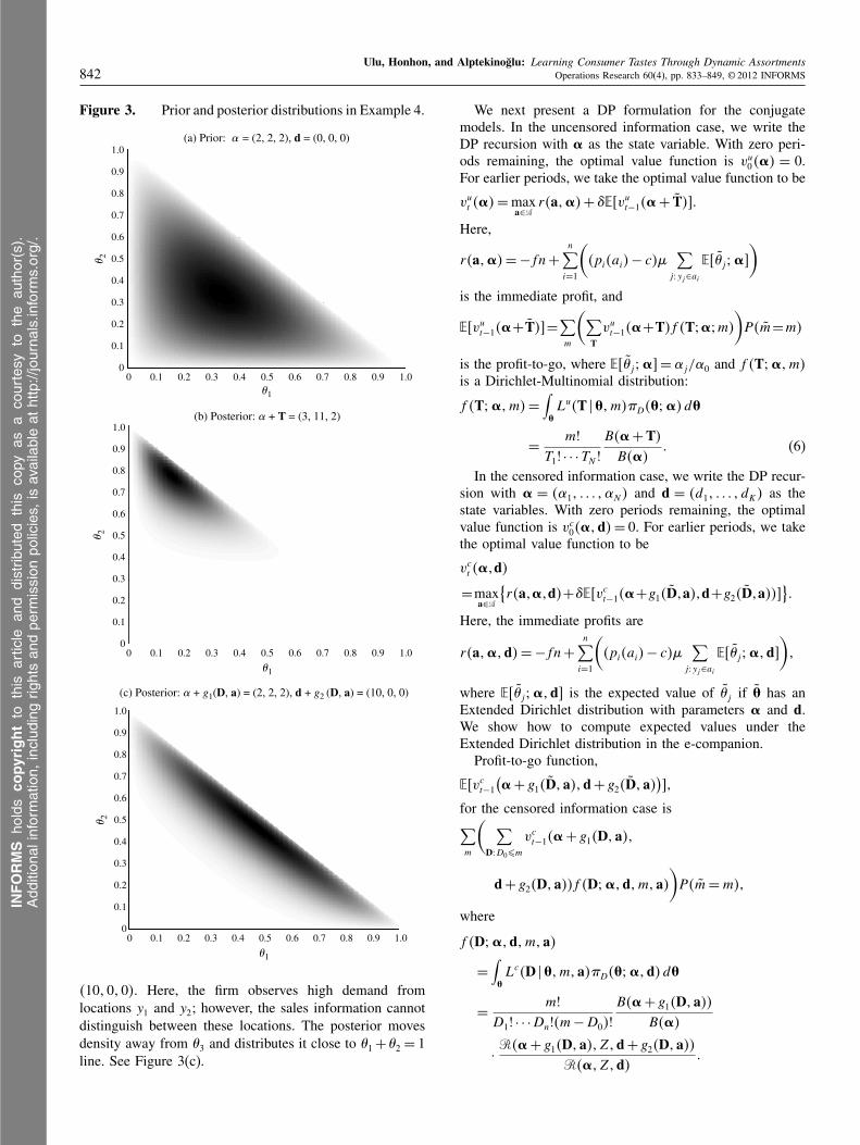
Example 4. Suppose there are three consumer locations,and let � be a Dirichlet distribution with parameters Á =

4212125. In the uncensored information case, if the firmreceives consumer taste information T = 4119105, then theposterior is a Dirichlet distribution with parameters Á +

T = 43111125. The prior and the posterior distributions areshown in Figures 3(a) and 3(b) on a unit simplex wheredarker regions correspond to points with higher probabil-ity density. Observing many consumers from location y2

leads the firm to move probability mass towards highervalues of �2.

Take the censored information case now, and supposethat the firm does not receive information on consumertastes but rather infers them from the sales of a singleproduct that covers the first two locations: a = 46y11 y275.If the sales of that product is 10 and the firm observesm = 10, then the firm’s posterior is an Extended Dirichletwith parameters Á + g14D5 = 4212125 and d + g24D5 =

INFORMS

holds

copyrightto

this

article

and

distrib

uted

this

copy

asa

courtesy

tothe

author(s).

Add

ition

alinform

ation,

includ

ingrig

htsan

dpe

rmission

policies,

isav

ailableat

http://journa

ls.in

form

s.org/.

Ulu, Honhon, and Alptekinoglu: Learning Consumer Tastes Through Dynamic Assortments842 Operations Research 60(4), pp. 833–849, © 2012 INFORMS

Figure 3. Prior and posterior distributions in Example 4.

1.00.90.80.70.60.5�1

�2

0.40.30.20.10

0

1.00.90.80.70.60.5

�1

0.40.30.20.10

1.00.90.80.70.60.5

�1

0.40.30.20.10

0.1

0.2

0.3

0.4

0.5

0.6

0.7

0.8

0.9

1.0

�2

0

0.1

0.2

0.3

0.4

0.5

0.6

0.7

0.8

0.9

1.0

�2

0

0.1

0.2

0.3

0.4

0.5

0.6

0.7

0.8

0.9

1.0

(a) Prior: � = (2, 2, 2), d = (0, 0, 0)

(b) Posterior: � + T = (3, 11, 2)

(c) Posterior: � + g1(D, a) = (2, 2, 2), d + g2 (D, a) = (10, 0, 0)

41010105. Here, the firm observes high demand fromlocations y1 and y2; however, the sales information cannotdistinguish between these locations. The posterior movesdensity away from �3 and distributes it close to �1 +�2 = 1line. See Figure 3(c).

We next present a DP formulation for the conjugatemodels. In the uncensored information case, we write theDP recursion with Á as the state variable. With zero peri-ods remaining, the optimal value function is vu04Á5 = 0.For earlier periods, we take the optimal value function to be

vut 4Á5= maxa∈A

r4a1Á5+ �Ɛ6vut−14Á+ T570

Here,

r4a1Á5= −fn+

n∑

i=1

(

4pi4ai5− c5�∑

j2 yj∈ai

Ɛ6�j3Á7

)

is the immediate profit, and

Ɛ6vut−14Á+T57=∑

m

(

∑

T

vut−14Á+T5f 4T3Á3m5

)

P4m=m5

is the profit-to-go, where Ɛ6�j3Á7= �j/�0 and f 4T3Á1m5is a Dirichlet-Multinomial distribution:

f 4T3Á1m5=

∫

ÈLu4T �È1m5�D4È3Á5dÈ

=m!

T1! · · ·TN !

B4Á+ T5B4Á5

0 (6)

In the censored information case, we write the DP recur-sion with Á = 4�11 0 0 0 1�N 5 and d = 4d11 0 0 0 1 dK5 as thestate variables. With zero periods remaining, the optimalvalue function is vc04Á1d5= 0. For earlier periods, we takethe optimal value function to be

vct 4Á1d5

=maxa∈A

{

r4a1Á1d5+�Ɛ6vct−14Á+g14D1a51d+g24D1a557}

0

Here, the immediate profits are

r4a1Á1d5= −fn+

n∑

i=1

(

4pi4ai5− c5�∑

j2 yj∈ai

Ɛ6�j3Á1d7)

1

where Ɛ6�j3Á1d7 is the expected value of �j if È has anExtended Dirichlet distribution with parameters Á and d.We show how to compute expected values under theExtended Dirichlet distribution in the e-companion.

Profit-to-go function,

Ɛ6vct−1

(

Á+ g14D1a51d + g24D1a5)

71

for the censored information case is∑

m

(

∑

D2D0¶m

vct−14Á+ g14D1a51

d + g24D1a55f 4D3Á1d1m1a5)

P4m=m51

where

f 4D3Á1d1m1a5

=

∫

ÈLc4D �È1m1a5�D4È3Á1d5dÈ

=m!

D1! · · ·Dn!4m−D05!

B4Á+ g14D1a55B4Á5

·R4Á+ g14D1a51Z1d + g24D1a55

R4Á1Z1d50

INFORMS

holds

copyrightto

this

article

and

distrib

uted

this

copy

asa

courtesy

tothe

author(s).

Add

ition

alinform

ation,

includ

ingrig

htsan

dpe

rmission

policies,

isav

ailableat

http://journa

ls.in

form

s.org/.

Ulu, Honhon, and Alptekinoglu: Learning Consumer Tastes Through Dynamic AssortmentsOperations Research 60(4), pp. 833–849, © 2012 INFORMS 843

This distribution is similar to the Dirichlet-Multinomial dis-tribution in (6) with the exception of the ratio of normaliz-ing constants that addresses the censoring.

In summary, using the conjugate models allows us tochange the state variable of the DP from a probability dis-tribution, �, to a finite-sized vector of size N in the uncen-sored case and of size N × 42N − N − 25 in the censoredcase. Furthermore, it allows us to reduce the infinite statespace of the original problem, that is, the set of all possibleprior distributions for each period, to a countably infinitestate space when the market size has infinite support or afinite state space when it has finite support.

5. Numerical StudyThe purpose of this section is twofold. First, we givesome numerical examples that compare optimal assort-ments under various multiperiod scenarios and highlightinteresting aspects of dynamic assortments that relate tothe exploration-exploitation trade-off. Second, we study thevalue of learning.

5.1. Exploration vs. Exploitation

To demonstrate the trade-off between learning and maxi-mizing immediate profits, we study five numerical exam-ples. In all cases, we set � = 1 and assume a Dirichlet orextended Dirichlet prior and a deterministic market size.We use short time horizons (t ¶ 3), few consumer locations(N = 3), and a small market size (m= 2) so that we can listall possible sales vectors and present the optimal dynamicassortment in compact tables. Consistent with the way ourDP formulation is laid out, we number periods backward:period 3 precedes period 2, and period 2 precedes period 1.As a shorthand, we write yi as opposed to 6yi1 yi7 when aproduct covers only one location.

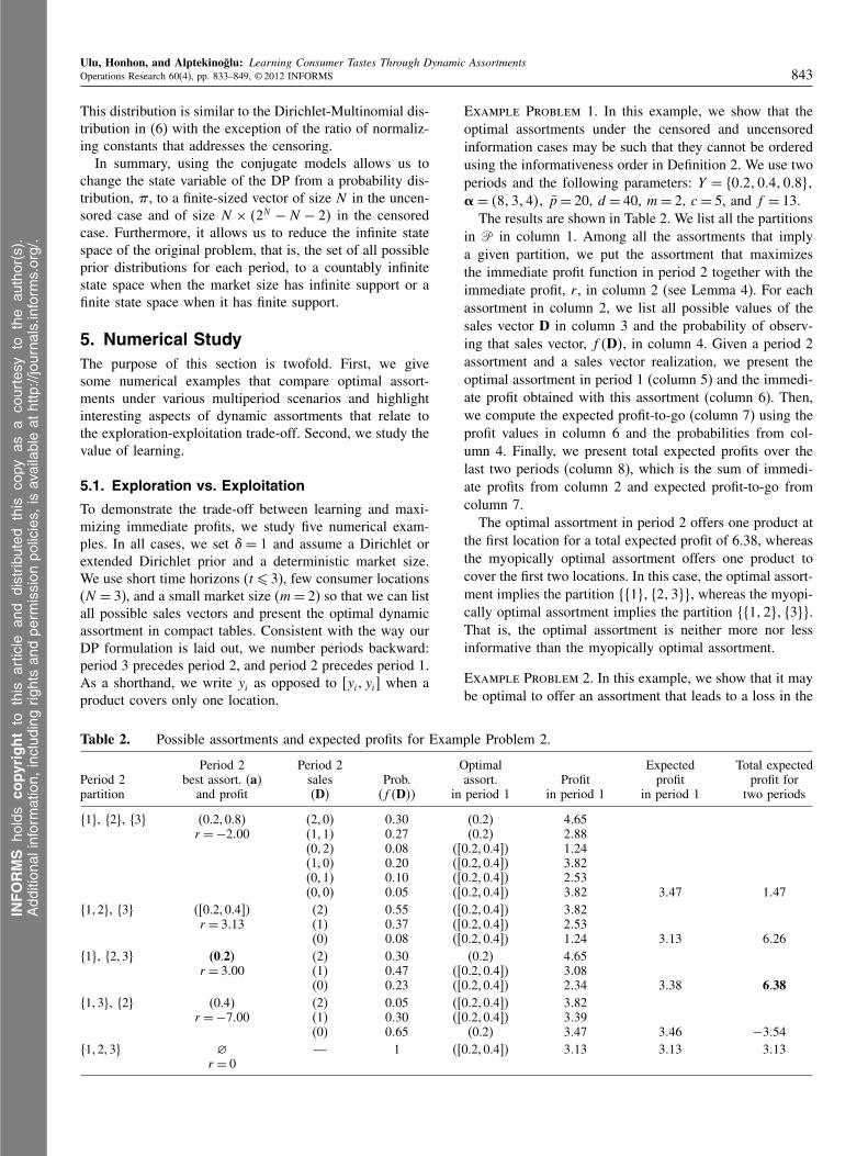
Table 2. Possible assortments and expected profits for Example Problem 2.

Period 2 Period 2 Optimal Expected Total expectedPeriod 2 best assort. (a) sales Prob. assort. Profit profit profit forpartition and profit (D) (f 4D5) in period 1 in period 1 in period 1 two periods

{1}, {2}, {3} (0.2, 0.8) (2, 0) 0030 (0.2) 4065r = −2000 (1, 1) 0027 (0.2) 2088

(0, 2) 0008 ([0.2, 0.4]) 1024(1, 0) 0020 ([0.2, 0.4]) 3082(0, 1) 0010 ([0.2, 0.4]) 2053(0, 0) 0005 ([0.2, 0.4]) 3082 3047 1047

{1, 2}, {3} ([0.2, 0.4]) (2) 0055 ([0.2, 0.4]) 3082r = 3013 (1) 0037 ([0.2, 0.4]) 2053

(0) 0008 ([0.2, 0.4]) 1024 3013 6026{1}, {2, 3} (0.2) (2) 0030 (0.2) 4065

r = 3000 (1) 0047 ([0.2, 0.4]) 3008(0) 0023 ([0.2, 0.4]) 2034 3038 6038

{1, 3}, {2} (0.4) (2) 0005 ([0.2, 0.4]) 3082r = −7000 (1) 0030 ([0.2, 0.4]) 3039

(0) 0065 (0.2) 3047 3046 −3054{1, 2, 3} � — 1 ([0.2, 0.4]) 3013 3013 3013

r = 0

Example Problem 1. In this example, we show that theoptimal assortments under the censored and uncensoredinformation cases may be such that they cannot be orderedusing the informativeness order in Definition 2. We use twoperiods and the following parameters: Y = 80021004100891Á= 48131451 p = 20, d = 40, m= 2, c = 5, and f = 13.

The results are shown in Table 2. We list all the partitionsin P in column 1. Among all the assortments that implya given partition, we put the assortment that maximizesthe immediate profit function in period 2 together with theimmediate profit, r , in column 2 (see Lemma 4). For eachassortment in column 2, we list all possible values of thesales vector D in column 3 and the probability of observ-ing that sales vector, f 4D5, in column 4. Given a period 2assortment and a sales vector realization, we present theoptimal assortment in period 1 (column 5) and the immedi-ate profit obtained with this assortment (column 6). Then,we compute the expected profit-to-go (column 7) using theprofit values in column 6 and the probabilities from col-umn 4. Finally, we present total expected profits over thelast two periods (column 8), which is the sum of immedi-ate profits from column 2 and expected profit-to-go fromcolumn 7.

The optimal assortment in period 2 offers one product atthe first location for a total expected profit of 6.38, whereasthe myopically optimal assortment offers one product tocover the first two locations. In this case, the optimal assort-ment implies the partition 88191 821399, whereas the myopi-cally optimal assortment implies the partition 8811291 8399.That is, the optimal assortment is neither more nor lessinformative than the myopically optimal assortment.

Example Problem 2. In this example, we show that it maybe optimal to offer an assortment that leads to a loss in the

INFORMS

holds

copyrightto

this

article

and

distrib

uted

this

copy

asa

courtesy

tothe

author(s).

Add

ition

alinform

ation,

includ

ingrig

htsan

dpe

rmission

policies,

isav

ailableat

http://journa

ls.in

form

s.org/.

Ulu, Honhon, and Alptekinoglu: Learning Consumer Tastes Through Dynamic Assortments844 Operations Research 60(4), pp. 833–849, © 2012 INFORMS

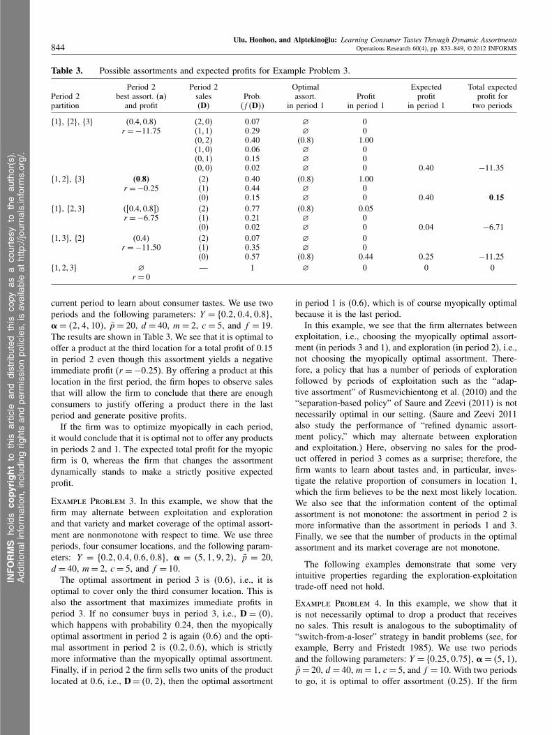
Table 3. Possible assortments and expected profits for Example Problem 3.

Period 2 Period 2 Optimal Expected Total expectedPeriod 2 best assort. (a) sales Prob. assort. Profit profit profit forpartition and profit (D) (f 4D5) in period 1 in period 1 in period 1 two periods

{1}, {2}, {3} (0.4, 0.8) (2, 0) 0007 � 0r = −11075 (1, 1) 0029 � 0

(0, 2) 0040 (0.8) 1.00(1, 0) 0006 � 0(0, 1) 0015 � 0(0, 0) 0002 � 0 0040 −11035

{1, 2}, {3} (0.8) (2) 0040 (0.8) 1.00r = −0025 (1) 0044 � 0

(0) 0015 � 0 0040 0015{1}, {2, 3} ([0.4, 0.8]) (2) 0077 (0.8) 0.05

r = −6075 (1) 0021 � 0(0) 0002 � 0 0004 −6071

{1, 3}, {2} (0.4) (2) 0007 � 0r = −11050 (1) 0035 � 0

(0) 0057 (0.8) 0.44 0025 −11025{1, 2, 3} � — 1 � 0 0 0

r = 0

current period to learn about consumer tastes. We use twoperiods and the following parameters: Y = 80021004100891Á = 42141105, p = 20, d = 40, m = 2, c = 5, and f = 19.The results are shown in Table 3. We see that it is optimal tooffer a product at the third location for a total profit of 0.15in period 2 even though this assortment yields a negativeimmediate profit (r = −0025). By offering a product at thislocation in the first period, the firm hopes to observe salesthat will allow the firm to conclude that there are enoughconsumers to justify offering a product there in the lastperiod and generate positive profits.

If the firm was to optimize myopically in each period,it would conclude that it is optimal not to offer any productsin periods 2 and 1. The expected total profit for the myopicfirm is 0, whereas the firm that changes the assortmentdynamically stands to make a strictly positive expectedprofit.

Example Problem 3. In this example, we show that thefirm may alternate between exploitation and explorationand that variety and market coverage of the optimal assort-ment are nonmonotone with respect to time. We use threeperiods, four consumer locations, and the following param-eters: Y = 80021004100610089, Á = 451119125, p = 20,d = 40, m= 2, c = 5, and f = 10.

The optimal assortment in period 3 is 40065, i.e., it isoptimal to cover only the third consumer location. This isalso the assortment that maximizes immediate profits inperiod 3. If no consumer buys in period 3, i.e., D = 405,which happens with probability 0.24, then the myopicallyoptimal assortment in period 2 is again 40065 and the opti-mal assortment in period 2 is 400210065, which is strictlymore informative than the myopically optimal assortment.Finally, if in period 2 the firm sells two units of the productlocated at 006, i.e., D = 40125, then the optimal assortment

in period 1 is 40065, which is of course myopically optimalbecause it is the last period.

In this example, we see that the firm alternates betweenexploitation, i.e., choosing the myopically optimal assort-ment (in periods 3 and 1), and exploration (in period 2), i.e.,not choosing the myopically optimal assortment. There-fore, a policy that has a number of periods of explorationfollowed by periods of exploitation such as the “adap-tive assortment” of Rusmevichientong et al. (2010) and the“separation-based policy” of Saure and Zeevi (2011) is notnecessarily optimal in our setting. (Saure and Zeevi 2011also study the performance of “refined dynamic assort-ment policy,” which may alternate between explorationand exploitation.) Here, observing no sales for the prod-uct offered in period 3 comes as a surprise; therefore, thefirm wants to learn about tastes and, in particular, inves-tigate the relative proportion of consumers in location 1,which the firm believes to be the next most likely location.We also see that the information content of the optimalassortment is not monotone: the assortment in period 2 ismore informative than the assortment in periods 1 and 3.Finally, we see that the number of products in the optimalassortment and its market coverage are not monotone.

The following examples demonstrate that some veryintuitive properties regarding the exploration-exploitationtrade-off need not hold.

Example Problem 4. In this example, we show that itis not necessarily optimal to drop a product that receivesno sales. This result is analogous to the suboptimality of“switch-from-a-loser” strategy in bandit problems (see, forexample, Berry and Fristedt 1985). We use two periodsand the following parameters: Y = 80025100759, Á= 45115,p = 20, d = 40, m= 1, c = 5, and f = 10. With two periodsto go, it is optimal to offer assortment 400255. If the firm

INFORMS

holds

copyrightto

this

article

and

distrib

uted

this

copy

asa

courtesy

tothe

author(s).

Add

ition

alinform

ation,

includ

ingrig

htsan

dpe

rmission

policies,

isav

ailableat

http://journa

ls.in

form

s.org/.

Ulu, Honhon, and Alptekinoglu: Learning Consumer Tastes Through Dynamic AssortmentsOperations Research 60(4), pp. 833–849, © 2012 INFORMS 845

sees zero sales, which happens with probability 0.17, thenit is still optimal to offer assortment 400255 with one periodto go. This is because the new observation is not enoughto counterbalance the prior distribution, which indicates astrong likelihood that most customers are in location 1.

Example Problem 5. In this example, we show that it maybe optimal to stop covering a consumer location even afterobserving the highest sales possible for the product thatcovers this location. This result is at odds with the “stay-with-a-winner” rule shown to be optimal in some banditproblems (Berry and Fristedt 1985). We use two periodsand the following parameters: Y = 8001100510075100959,Á = 411212145, d = 401 0 0 0 1013101 0 0 0 105 where 3 is thevalue of parameter d that corresponds to censoring oflocations 3 and 4, p = 20, d = 40, m = 3, c = 5, andf = 10. With two periods to go, the optimal assortment is46005100757100955. If the firm sells three units of the prod-uct that covers locations 2 and 3, which happens with prob-ability 0.1034, the optimal assortment with one period togo becomes 4600751009575; that is, location 2 is no longercovered.

5.2. Value of Learning

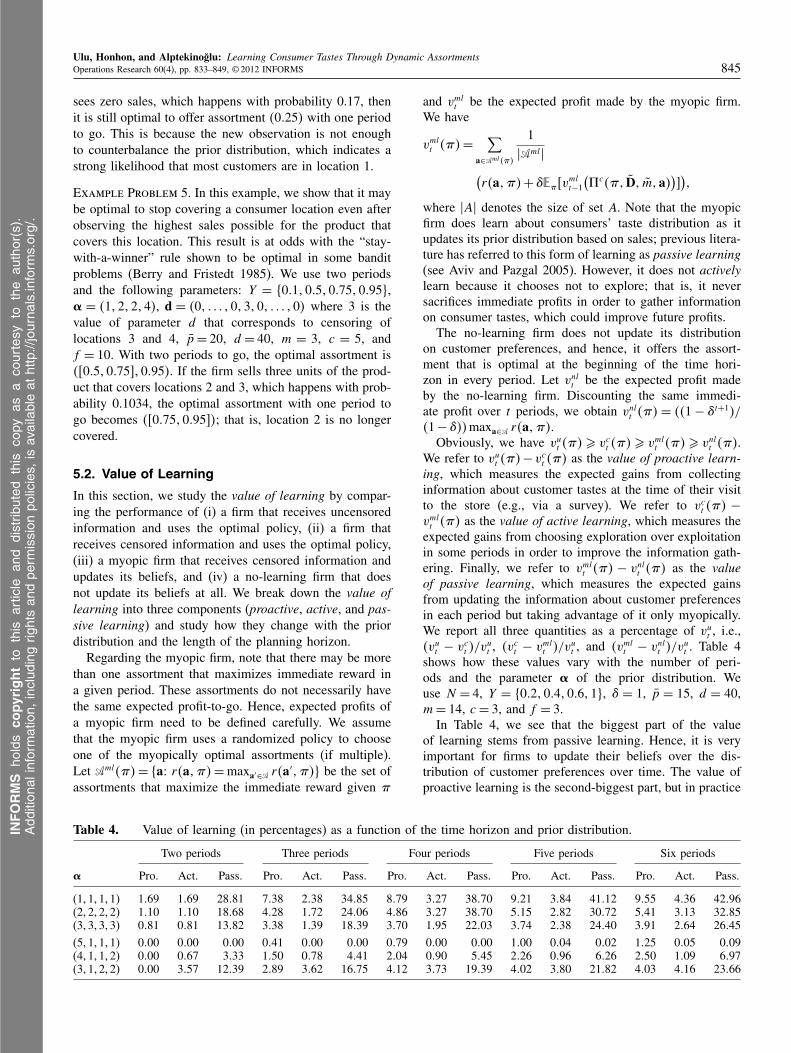
In this section, we study the value of learning by compar-ing the performance of (i) a firm that receives uncensoredinformation and uses the optimal policy, (ii) a firm thatreceives censored information and uses the optimal policy,(iii) a myopic firm that receives censored information andupdates its beliefs, and (iv) a no-learning firm that doesnot update its beliefs at all. We break down the value oflearning into three components (proactive, active, and pas-sive learning) and study how they change with the priordistribution and the length of the planning horizon.

Regarding the myopic firm, note that there may be morethan one assortment that maximizes immediate reward ina given period. These assortments do not necessarily havethe same expected profit-to-go. Hence, expected profits ofa myopic firm need to be defined carefully. We assumethat the myopic firm uses a randomized policy to chooseone of the myopically optimal assortments (if multiple).Let Aml4�5= 8a2 r4a1�5= maxa′∈A r4a

′1�59 be the set ofassortments that maximize the immediate reward given �

Table 4. Value of learning (in percentages) as a function of the time horizon and prior distribution.

Two periods Three periods Four periods Five periods Six periods

Á Pro. Act. Pass. Pro. Act. Pass. Pro. Act. Pass. Pro. Act. Pass. Pro. Act. Pass.

(1, 1, 1, 1) 1069 1069 28081 7038 2038 34085 8079 3027 38070 9021 3084 41012 9055 4036 42096(2, 2, 2, 2) 1010 1010 18068 4028 1072 24006 4086 3027 38070 5015 2082 30072 5041 3013 32085(3, 3, 3, 3) 0081 0081 13082 3038 1039 18039 3070 1095 22003 3074 2038 24040 3091 2064 26045

(5, 1, 1, 1) 0000 0000 0000 0041 0000 0000 0079 0000 0000 1000 0004 0002 1025 0005 0009(4, 1, 1, 2) 0000 0067 3033 1050 0078 4041 2004 0090 5045 2026 0096 6026 2050 1009 6097(3, 1, 2, 2) 0000 3057 12039 2089 3062 16075 4012 3073 19039 4002 3080 21082 4003 4016 23066

and vmlt be the expected profit made by the myopic firm.

We have

vmlt 4�5=

∑

a∈Aml4�5

1�Aml�

(

r4a1�5+ �Ɛ�6vmlt−1

(

çc4�1 D1 m1a5)

7)

1

where �A� denotes the size of set A. Note that the myopicfirm does learn about consumers’ taste distribution as itupdates its prior distribution based on sales; previous litera-ture has referred to this form of learning as passive learning(see Aviv and Pazgal 2005). However, it does not activelylearn because it chooses not to explore; that is, it neversacrifices immediate profits in order to gather informationon consumer tastes, which could improve future profits.

The no-learning firm does not update its distributionon customer preferences, and hence, it offers the assort-ment that is optimal at the beginning of the time hori-zon in every period. Let vnlt be the expected profit madeby the no-learning firm. Discounting the same immedi-ate profit over t periods, we obtain vnlt 4�5 = 441 − �t+15/41 − �55maxa∈A r4a1�5.

Obviously, we have vut 4�5 ¾ vct 4�5 ¾ vmlt 4�5 ¾ vnlt 4�5.

We refer to vut 4�5− vct 4�5 as the value of proactive learn-ing, which measures the expected gains from collectinginformation about customer tastes at the time of their visitto the store (e.g., via a survey). We refer to vct 4�5 −

vmlt 4�5 as the value of active learning, which measures the

expected gains from choosing exploration over exploitationin some periods in order to improve the information gath-ering. Finally, we refer to vml

t 4�5 − vnlt 4�5 as the valueof passive learning, which measures the expected gainsfrom updating the information about customer preferencesin each period but taking advantage of it only myopically.We report all three quantities as a percentage of vut , i.e.,4vut − vct 5/v

ut , 4vct − vml

t 5/vut , and 4vmlt − vnlt 5/v

ut . Table 4

shows how these values vary with the number of peri-ods and the parameter Á of the prior distribution. Weuse N = 4, Y = 800210041006119, � = 1, p = 15, d = 40,m= 14, c = 3, and f = 3.

In Table 4, we see that the biggest part of the valueof learning stems from passive learning. Hence, it is veryimportant for firms to update their beliefs over the dis-tribution of customer preferences over time. The value ofproactive learning is the second-biggest part, but in practice

INFORMS

holds

copyrightto

this

article

and

distrib

uted

this

copy

asa

courtesy

tothe

author(s).

Add

ition

alinform

ation,

includ

ingrig

htsan

dpe

rmission

policies,

isav

ailableat

http://journa

ls.in

form

s.org/.

Ulu, Honhon, and Alptekinoglu: Learning Consumer Tastes Through Dynamic Assortments846 Operations Research 60(4), pp. 833–849, © 2012 INFORMS

it requires an important investment in resources becauseone would need to question every customer who exits thestore in order to know which product they truly wantedto buy (which may differ from the one they bought). Thevalue of active learning is the smallest of all three, but itremains significant, especially when the number of periodsis large. We see that as the number of periods increases,all three measures of the value of learning increase. Thisshows that as the time horizon expands, there might bea greater incentive to learn about consumer preferences.From looking at the first three rows, we also see that as thesum of the Á vector increases while keeping all �is equal,all three measures of the value of learning decrease. Thisis because �0 =

∑Ni=1 �i can be interpreted as the number

of past uncensored data points. The larger this number is,the more confident the firm is about the distribution of con-sumer tastes, therefore, the less it needs to learn. In the lastthree rows, we vary the prior distribution while keeping�0 constant, which means that we change firm’s beliefs onthe relative likelihood of the four consumer locations. Wefind that the relationship is not always monotone, but wegenerally find that the value of learning tends to be higherwhen the firm’s beliefs on the consumers’ taste distribu-tion is more diffuse, i.e., when the � vector is more evenlydistributed. This is because, in that case, there is a greaterpotential for learning compared to the case when the firmis already convinced that most of the customers are in oneend of the attribute space.

6. ExtensionsIn this section we discuss three extensions to our model:(i) unknown consumer locations, (ii) heterogenous reserva-tion price, and (iii) unobservable market size.

Unknown Consumer Locations. Our model assumes thatthe firm knows the discrete set of possible consumer loca-tions, Y , and is learning about the relative likelihood ofconsumers in the population being at each of these loca-tions. If there were consumer locations that the firm doesnot know about (outside of Y ), then it would not be able tolearn about their relative likelihood. We suggest two waysof handling this issue.

First, one could pick a very large set Y . For most practi-cal purposes, the domain of consumer locations is discrete.Take the example of milk. Consumers can only discern dif-ferences in fat content beyond a certain value, which canbe used to discretize the attribute space (e.g., 0.5%, 1%,1.5%, 2%, 2.5%). There are many other limits to humanperception, such as ability to differentiate colors, that setultimate limits on the level of granularity needed on prod-uct attributes. By assigning a very small (though positive)mass on each of these potential locations, the firm wouldbe able to learn about their relative probabilities. Althoughthis approach is challenging computationally when Y islarge, the model and insights developed in this paper wouldstill apply.

Alternatively, one can treat the distribution of consumertastes as continuous. This way, Bayesian updating candetermine which locations have higher posterior density.The problem with this approach is that there does not exista procedure to solve for the optimal assortment explicitly.As an approximation, one could divide the attribute spaceinto a fixed number of disjoint intervals and define �j asthe probability mass over the jth interval rather than atone point. The assortment problem becomes one of cov-ering intervals with products, i.e., a product can coverone or more adjacent intervals and its price can be setappropriately. Our entire analysis extends to this setting.Alptekinoglu et al. (2012) show that this approximationmethod performs very well even with a small number ofintervals: in most cases, it is possible to achieve 95% of theoptimal expected profit in single-period settings by dividingthe attribute space into only 10 intervals.

We also test our model for robustness in case of amisspecification of the set of consumer locations. Morespecifically, we assume that Z = 8z11 0 0 0 1 zS9 is the set ofconsumer locations, but that the firm thinks consumers arelocated in Y = 8y11 0 0 0 1 yN 9 where Y ⊆ Z, that is, the firmis missing some consumer locations. First, note that thefirm may capture sales from customers located in Z\Y ,but incorrectly attribute those sales to customers in Y .For example, suppose that Z = 800251005100759 and Y =

80025100759. If the firm offers assortment 4600251007575 andone customer from the central location comes to the store,the firm will sell a unit of the product but will wronglyinterpret this sales as coming from a customer located at0.25 or 0.75.

We numerically evaluate the impact of such misspecifi-cation on a firm’s expected profit. In period t, we (i) calcu-late the optimal assortment a = 4a11 0 0 0 1 an5 by solving forvct , (ii) simulate the demand D = 4D11 0 0 0 1Dn5 using thetrue distribution of customers, (iii) calculate the realizedprofit equal to −fn+

∑ni=14pi4ai5− c5Di, and (iv) update

the prior distribution as described in §4.4. We do so fortwo periods, then add up the realized profits to obtain thetwo-period realized profit value (we found that the insightsdid not change as we increased the number of periods). Werepeat this process over 10,000 instances and calculate theaverage two-period profit value.

We use S = 3, N = 2, Z = 800251005100759, � = 1,p = 25, d = 40, f = 10, and c = 3. The market size isunobservable5 and can be equal to 1 or 2 with equal prob-ability. For the true distribution of customer tastes we useÈ = 4�11 �21 �35 = 4436 − p5/721 p/361 436 − p5/725 wherep ∈ 821416181101129. We consider two cases: Y = Z andY = 80025100759. When Y =Z, we use Á= 36È and whenY ⊂Z, we use Á= 4436−p5/21 436−p5/25, so that in bothcases, the � vector of the prior distribution is proportionalto the È vector from the true distribution. The percent-age loss in average two-period profit with Y = 80025100759compared to Y = Z is 0, 0.31, 1.94, 9.32, 15.69, 21.42

INFORMS

holds

copyrightto

this

article

and

distrib

uted

this

copy

asa

courtesy

tothe

author(s).

Add

ition

alinform

ation,

includ

ingrig

htsan

dpe

rmission

policies,

isav

ailableat

http://journa

ls.in

form

s.org/.

Ulu, Honhon, and Alptekinoglu: Learning Consumer Tastes Through Dynamic AssortmentsOperations Research 60(4), pp. 833–849, © 2012 INFORMS 847

when p = 2, 4, 6, 8, 10, 12, respectively. As p increases,it becomes more likely that customers are located in thecenter location. We see that, as expected, the profit lossdue to misspecification increases as the missing locationbecomes more likely. In practice, the firm should have agood idea of where most of the customers are, imply-ing that missing locations should have a low probability.In such instances, we would not expect the impact of mis-specification to be significant.

Heterogenous Reservation Price. Next, we discuss theassumption of a fixed and known reservation price p. Sup-pose, instead, that consumers belong to two segments: thosewith a high (H ) reservation price, pH , and those with a low(L) reservation price, pL, with (known) respective prob-abilities � and 1 − �. In this case, one can define anassortment as a = 4aH 1aL5 where aH = 4aH

1 1 0 0 0 1 aHn 5 =

46xH1 1 x

H1 71 0 0 0 1 6x

Hn 1 x

Hn 75 are the high-type market seg-

ments and aL = 4aL1 1 0 0 0 1 a

Ln5= 46xL

1 1 xL1 71 0 0 0 1 6x

Ln 1 x

Ln 75 are

the low-type market segments. The introduction of het-erogeneous reservation price makes this problem consider-ably more complex; however, we show in the e-companionto this paper that our results—in particular Theorem 1—extend to this case, provided we redefine the informative-ness order over assortments as follows.

Let P4a5 be a partition on Y × 8H1L9, which containsn subsets of Y × 8H1L9, each of which corresponds toa distinct group of consumer locations and types coveredby one product in a, plus possibly one more subset thatcontains all the remaining consumer locations and types(if any) that are not covered. For example, if there are twoconsumer locations and aH = 46y11 y275 and aL = 46y11 y175,then P4a5= 884y11L51 4y11H51 4y21H591 84y21L599.

Definition 3. Assortment a = 4aH 1aL5 is “more informa-tive” than assortment a′ = 4a′H 1a′L5, or a �I a′, if P4a5 isa finer partition than P4a′5.

This definition generalizes our previous definition ofinformativeness. For an assortment to be more informative,implied partitions on locations and types need to be finer.

Unobservable Market Size. Our model assumes that thefirm is able to observe the market size together with theconsumer taste vector (in the uncensored information case)or the sales vector (in the censored information case).In practice, the firm may not be able to count the number ofconsumers who come to the store but leave empty-handed(this is especially true for brick-and-mortar stores). Havingto infer consumer tastes from sales only, the firm needsto take into account the additional uncertainty created bythe market size. For example, with three consumer loca-tions, if the market size is observable, 46y11 y171 6y21 y275 isas informative an assortment as 46y11 y171 6y21 y271 6y31 y375,because the firm can infer the number of consumers at loca-tion y3 even if it is not covered. However, when the marketsize is unobservable, the former is strictly less informa-

tive, which makes it necessary to redefine the notion ofinformativeness.

Definition 4. Assortment a = 4a11 0 0 0 1 an5 is (strictly)“strongly more informative” than assortment a′ =

4a′11 0 0 0 1 a

′n′5, or (a �SI a′) a �SI a′, if P4a5 is a (strictly)

finer partition than P4a′5, and assortment a covers morelocations than assortment a′, or

⋃n′

i′=1 a′i′ ⊆

⋃ni=1 ai.

We show in the e-companion to this paper that ourresults—in particular Theorem 1—extend to the caseof unobservable market size, provided we redefine theinformativeness order over assortments as in Defini-tion 4. Clearly, this definition implies our previous defi-nition (Definition 2) and imposes a stronger partial order.An assortment a that is more informative than a′ under theprevious definition is not necessarily more informative thana′ under this definition. Increasing the number of productswithin a group in Figure 2 increases the informativenesswhen the market size is unobservable, which can be shownto hold in general. Moreover, a strongly more informativeassortment contains higher variety (see Lemma EC.3 in thee-companion).

7. ConclusionIn this paper, we develop a model of dynamic assortmentplanning for horizontally differentiated products when aretailer is learning about consumer tastes. We study howthe firm should adjust assortments over time so as to learnconsumer tastes better. The classic exploration-exploitationtrade-off is present in our model: the firm may chooseto forgo immediate profits to learn about consumer tastes,which would help the firm in the coming periods.

We model horizontal differentiation on a Hotelling linewhere there is a finite number of locations (discrete points)that represent consumers’ ideal products or tastes. A firmoffers an assortment of products on the Hotelling line, set-ting their locations and prices, and paying a fixed cost perproduct. Each consumer has a choice to buy one unit ofa product that the firm offers or opt for an outside option.We study the firm’s assortment decisions in single- andmultiperiod settings. We highlight especially the learningaspect of assortments: over multiple periods, with dynam-ically changing assortments, the firm is able to infer con-sumer locations (perfectly or imperfectly) from past salesdata, learn their tastes better, and use this information tofine-tune its offering.

First, we show that the firm’s product location and pric-ing problem in the single-period case simplifies to a searchfor the optimal product market segments and that there isonly a finite number of possible assortments to consider.

Next, we introduce a multiperiod model with learning,and study the optimal assortment and pricing decisionsin this dynamic setting. We emphasize how sales of agiven assortment may provide the firm with censored infor-mation on consumer tastes. Intuitively, if the firm caters

INFORMS

holds

copyrightto

this

article

and

distrib

uted

this

copy

asa

courtesy

tothe

author(s).

Add

ition

alinform

ation,

includ

ingrig

htsan

dpe

rmission

policies,

isav

ailableat

http://journa

ls.in

form

s.org/.

Ulu, Honhon, and Alptekinoglu: Learning Consumer Tastes Through Dynamic Assortments848 Operations Research 60(4), pp. 833–849, © 2012 INFORMS

to many types of consumers with a single product, con-sumers substitute away from their ideal product and thefirm receives censored information about their tastes. Onthe other hand, if a firm offers many dedicated products,fewer consumers need to substitute away from ideal prod-ucts and the firm may gather better information aboutconsumer tastes. We formalize the notion of how informa-tive an assortment is and construct a partial order based onit. Depending on what the firm can infer about consumertastes from past sales data, some assortments are more infor-mative than others (e.g., at the extreme, offering a producttargeted for each possible consumer location is the mostinformative assortment). Using our partial order, we estab-lish the following result: it cannot be optimal for the firm toselect a less informative assortment than the optimal assort-ment under uncensored information (i.e., myopically opti-mal assortment). This is reminiscent of the “stock more”result shown in censored newsvendor settings where salesare observed, but not demand (see for example Ding et al.2002). This result is robust as it extends to the case of unob-servable market size and heterogenous reservation price pro-vided that one redefines the informativeness order of assort-ments carefully.

As an important special case of our multiperiod model,we also develop a family of conjugate learning models,using the Dirichlet and Extended Dirichlet distributions.We then present a number of numerical examples usingthese conjugate models and highlight interesting propertiesof the optimal dynamic assortments and value of learningover multiple periods. For instance, it is possible that theoptimal assortment may bring losses to the firm in earlyperiods, a phenomenon entirely driven by the firm’s desireto learn about consumer tastes.

We believe that the concept of dynamic assortmentsoffers rich analytical and empirical challenges to research-ers. For instance, exploring demand learning issues withalternative consumer choice models (e.g., preference rank-ing models) and possibly for products with multipleattributes would expand the applicability of insights gath-ered in the literature so far. Competition between firmslearning through dynamic assortment also remains largelyunexplored (in contrast, competition with “static assort-ment” has been studied, e.g., Alptekinoglu and Corbett2008). Building on our model, we think allowing con-sumer heterogeneity on transportation cost, modeling non-stationary consumer preferences, or treating the case wherethe firm learns about consumer tastes and the market sizesimultaneously, are all interesting and challenging prob-lems. Another interesting avenue for future research is toconsider the case where the firm holds inventory of theproducts and is not able to observe lost sales. In this case,there are two types of censoring: the censoring of consumertastes due to (assortment-based) substitution and the cen-soring of the market size and product demands due to thestockouts, and it will be interesting to study the interactionbetween them.

Electronic Companion

An electronic companion to this paper is available as part of theonline version at http://dx.doi.org/10.1287/opre.1120.1067.

Endnotes

1. Not every partition of Y is feasible, because each market seg-ment is a closed interval on ì (Lemma 1). In a partition inducedby an assortment, we can have at most one subset with nonadja-cent locations; that subset is the one with consumer locations (ifany) that are not covered.2. Chen and Plambeck (2008) show that in a multiperiodBayesian inventory management problem with nonperishableinventory, the optimal inventory level may be lower than themyopic level because reducing inventory helps mitigate risk ofoverstocking in subsequent periods.3. Because of this partial order “not less informative” is not thesame as “at least as informative.”4. Each column has at least two 1s, and column k means thatthe subset of locations Yk ≡ 8yj 2 Zjk = 19 belongs to at least onefeasible partition P ∈ P. Column k is relevant only when theassortment contains a product that exactly covers all locations inYk or when the assortment leaves all locations in Yk not covered.5. If the market size was observable, the firm who uses Y ⊂ Z

would understand that some consumer locations are missing whenit believes its current assortment covers the whole market butobtains a total sales lower than m.

Acknowledgments

The authors are grateful for helpful comments provided by JimSmith, Sridhar Seshadri, and the anonymous associate editor andreferees.

ReferencesAlptekinoglu A, Corbett CJ (2008) Mass customization vs. mass pro-

duction: Variety and price competition. Manufacturing Service Oper.Management 10(2):204–217.

Alptekinoglu A, Corbett CJ (2010) Leadtime-variety tradeoff inproduct differentiation. Manufacturing Service Oper. Management12(4):569–582.

Alptekinoglu A, Honhon D, Ulu C (2012) Positioning and pricing of hor-izontally differentiated products. Working paper, Southern MethodistUniversity, Dallas.

Aviv Y, Pazgal A (2005) Dynamic pricing of short life-cycle prod-ucts through active learning. Working paper, Washington University,St. Louis.

Bernstein F, Kök AG, Xie L (2011) Dynamic assortment customiza-tion with limited inventories. Working paper, Duke University,Durham, NC.

Berry DA, Fristedt B (1985) Bandit Problems: Sequential Allocation ofExperiments (Chapman & Hall, London).

Caldentey R, Caro F (2010) Dynamic assortment planning. Working paper,New York University, New York.

Caro F, Gallien J (2007) Dynamic assortment with demand learning forseasonal consumer goods. Management Sci. 53(2):276–292.

Caro F, Martinez-de-Albeniz V (2012) Product and price competition withsatiation effects. Management Sci. 58(7):1357–1373.

Chen F, Eliashberg J, Zipkin P (1998) Customer preferences, supply-chaincosts, and product-line design. Ho T-H, Tang CS, eds. Product Vari-ety Management: Research Advances (Kluwer Academic Publishers,Norwell, MA), 123–144.

INFORMS

holds

copyrightto

this

article

and

distrib

uted

this

copy

asa

courtesy

tothe

author(s).

Add

ition

alinform

ation,

includ

ingrig

htsan

dpe

rmission

policies,

isav

ailableat

http://journa

ls.in

form

s.org/.

Ulu, Honhon, and Alptekinoglu: Learning Consumer Tastes Through Dynamic AssortmentsOperations Research 60(4), pp. 833–849, © 2012 INFORMS 849

Chen L, Plambeck EL (2008) Dynamic inventory management with learn-ing about the demand distribution and substitution probability. Man-ufacturing Service Oper. Management 10(2):126–156.

Dickey JM, Jiang J, Kadane JB (1987) Bayesian methods for censoredcategorical data. J. Amer. Statist. Assoc. 82(399):773–781.

Ding X, Puterman ML, Bisi A (2002) The censored newsvendor and theoptimal acquisition of information. Oper. Res. 50(3):517–527.

Gaur V, Honhon D (2006) Product variety and inventory decisionsunder a locational consumer choice model. Management Sci. 52(10):1528–1543.

Harpaz G, Lee WY, Winkler RL (1982) Learning, experimentation, andthe optimal output decisions of a competitive firm. Management Sci.28(6):589–603.

Hotelling H (1929) Stability in competition. Econom. J. 39(153):41–57.Kök AG, Fisher M, Vaidyanathan R (2009) Assortment planning: Review

of literature and industry practice. Agrawal N, Smith SA, eds. RetailSupply Chain Management (Springer, New York), 99–153.

Lancaster K (1966) A new approach to consumer theory. J. PoliticalEconom. 74(2):132–157.

Lu X, Song J, Zhu K (2005) On “the censored newsvendor and the optimalacquisition of information.” Oper. Res. 53(6):1024–1027.

Olivares O, Lu Y, Musalem A, Schilkrut A (2011) Measuring the effect ofqueues on customer purchases. Working paper, Columbia University,New York.

Rusmevichientong P, Shen M, Shmoys D (2010) Dynamic assortmentoptimization with a multinomial logit choice model and capacity con-straint. Oper. Res. 58(6):1666–1680.

Saure D, Zeevi A (2011) Optimal dynamic assortment planning withdemand learning. Working paper, Columbia University, New York.

Canan Ulu is an assistant professor in the Information, Riskand Operations Management Department at the McCombs Schoolof Business, University of Texas at Austin. Her research interestsinclude Bayesian learning in sequential decision problems and theimpact of behavioral decision theory on decision analysis methods.

Dorothée Honhon is an assistant professor in the Departmentof Industrial Engineering at the Eindhoven University of Technol-ogy in the Netherlands. Her research interests include inventorymanagement, assortment planning, retail operations, behavioraloperations management, and transportation theory.

Aydin Alptekinoglu is an assistant professor of operationsmanagement at Cox School of Business, Southern Methodist Uni-versity. His broad research interest is product strategy. He studiesproduct variety management, assortment planning, customizationof goods and services, retail returns, and other aspects of productstrategy that lie at the interface of operations and marketing.

INFORMS

holds

copyrightto

this

article

and

distrib

uted

this

copy

asa

courtesy

tothe

author(s).

Add

ition

alinform

ation,

includ

ingrig

htsan

dpe

rmission

policies,

isav

ailableat

http://journa

ls.in

form

s.org/.