Learning and RBF

8/2/2019 Learning and RBF

http://slidepdf.com/reader/full/learning-and-rbf 1/32

Learning and RBF

Page 46

Heteroassociative memories are composed of two layers of linear units—an input layer

and an output layer—connected by a set of modifiable connections. They differ fromautoassociative memories in that an input pattern is associated to an output pattern

instead of being associated to itself. The goal of a heteroassociative memory is to learn

mappings between input-output pairs such that the memory produces the appropriateoutput in response to a given input pattern.

Heteroassociative memories are generally used to solve pattern identification and

categorization problems. They differ from the perceptron presented in Chapter 2 in thattheir basic units are linear and their input and output continuous. From a statistical pointof view the inner working of a heteroassociative memory is equivalent to the technique

of multiple linear regression and can be analyzed using the mathematical tools detailed

in the chapter on autoassociative memories (i.e., least squares estimation and eigen- orsingular value decomposition). From a cognitivist point of view, their interest comes

Page 47

Figure 4.1:

Responses of a heteroassociative memory trained to associate frontal and

profile views of 20 female faces. The top row represents the images

presented as memory keys and the bottom row the images reconstructed



by the memory. The association between the frontal view and the profile

view at the extreme left was learned. The other associations were not learned.

from the fact that they provide a way of simulating the associative properties of human

memories.

As an application example, Fig. 4.1 illustrates the performance of a heteroassociative

memory trained to associate frontal and profile views of 20 female faces.1 After learningcompletion, the ability of the memory to produce profile views of learned faces in

response to a frontal or a 3/4 view of the faces was evaluated along with the memory's

ability to generalize to new faces. For a learned face (left panels), the memory responseto the input of a frontal view is an exact profile view, but the response to a 3/4 view is

only an approximate profile view. For faces not learned (right panels), the quality of the

profile approximation decreases.

4.2 Architecture of a Heteroassociative Memory

The building blocks of linear heteroassociative memories are the basic linear unitsdescribed in Chapter 3 (see illustration Fig. 3.2 on page 22). Specifically, a linear

heteroassociative memory is a network composed of I input units connected to J output

units. Each output units receives inputs from all the input units, sums them, andtransforms the sum into a response via a linear transfer function. The set

1The face images were represented as vectors of pixel intensities obtained by concatenation of the

columns of digitized photographic images.

Page 48



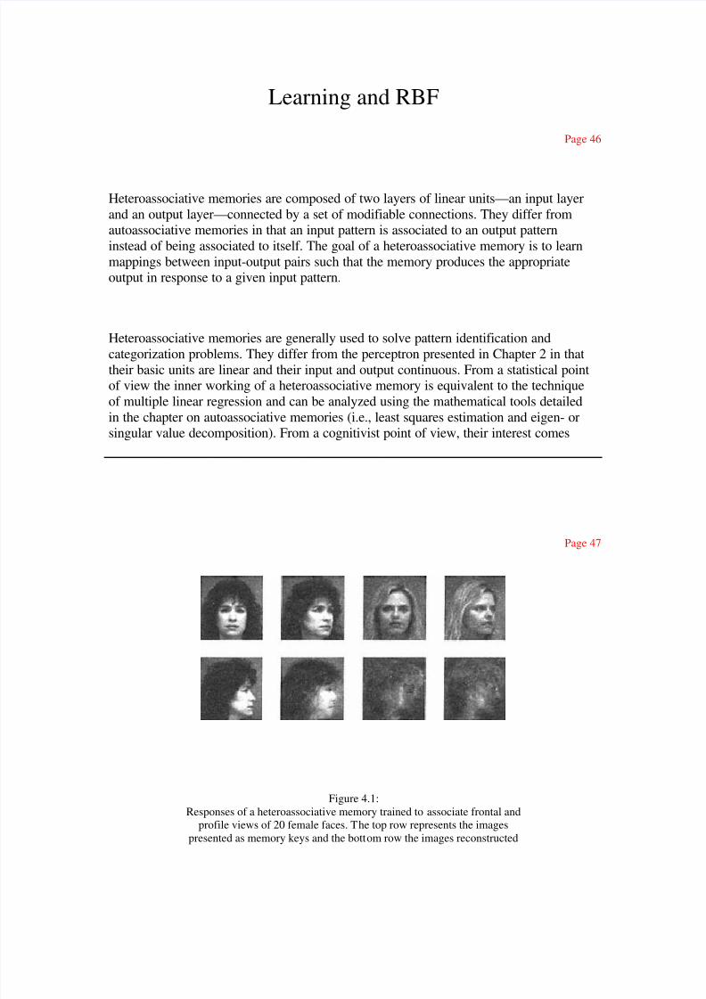
Figure 4.2: Architecture of a heteroassociative memory.

of connections between input and output units is represented by an I × J matrix W:

In this matrix, a given element wi,j represents the strength of the connection between the

ith input unit and the jth output unit.

Each of the K input patterns is represented by an I -dimensional vector denoted xk . Each

of the K corresponding output patterns is represented by a J -dimensional vector denoted

tk . The set of K input patterns is represented by an I × K matrix denoted X in which the

k th column corresponds to the k th input vector xk . Likewise, the set of K output patterns

is represented by a J × K matrix denoted T in which the k th column corresponds to the

k th output vector tk . Learning of the mapping between input-output pairs is done by

modifying the strength of the connections between input and output units. Thesemodifications can be implemented using the two learning rules described in Chapter 3

(i.e., Hebbian and Widrow-Hoff).

4.3 The Hebbian Learning Rule



Remember that Hebb's learning rule states that the strength of the synapse between twoneurons is a function of the temporal correlation between the two neurons (e.g., it

increases whenever they fire simultaneously). In a heteroassociative memory:

Page 49

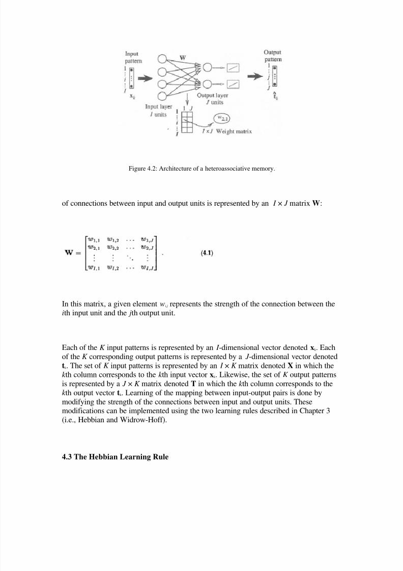
Figure 4.3:

Face-name pairs to be stored in a heteroassociative memory.

The Hebbian learning rule sets the change of the connection weights to be proportional to the

product of the input and the expected output .

Formally, a set of K input-output pairs is stored in a heteroassociative memory by multiplyingeach input pattern vector by the corresponding output pattern vector and summing the resulting

outer-product matrices. Specifically, the connection weight matrix is obtained with Hebbian

learning as



where γ represents the proportionality constant. Note that, in this case, the Hebbian learning rulecould be considered as a supervised type of learning because the correct output is used during

learning. A completely unsupervised version of this rule also exists in which the actual outputvector is associated with the input vector instead of the expected output. This version of the ruleis, however, seldom used (see Hagan, Demuth, & Beale, 1996, for some examples).

4.3.1 Numerical Example: Face and Name Association

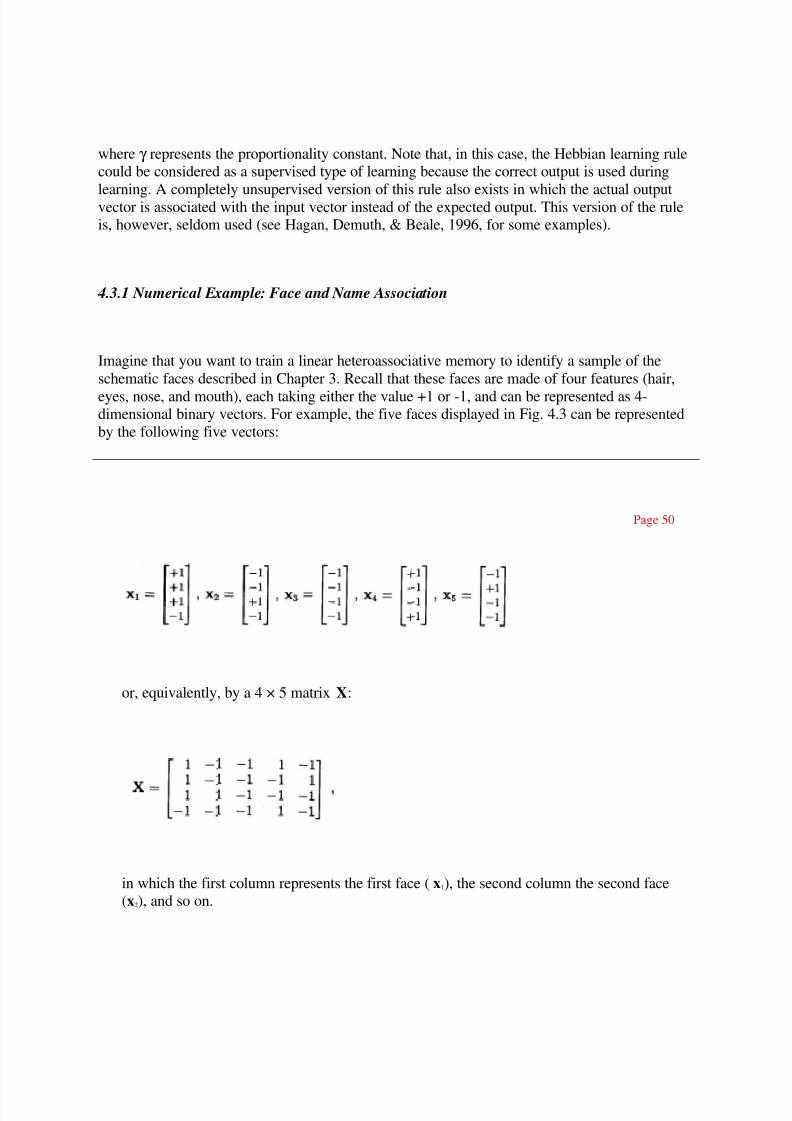
Imagine that you want to train a linear heteroassociative memory to identify a sample of the

schematic faces described in Chapter 3. Recall that these faces are made of four features (hair,

eyes, nose, and mouth), each taking either the value +1 or -1, and can be represented as 4-dimensional binary vectors. For example, the five faces displayed in Fig. 4.3 can be represented

by the following five vectors:

Page 50

or, equivalently, by a 4 × 5 matrix X:

in which the first column represents the first face (x1), the second column the second face(x2), and so on.



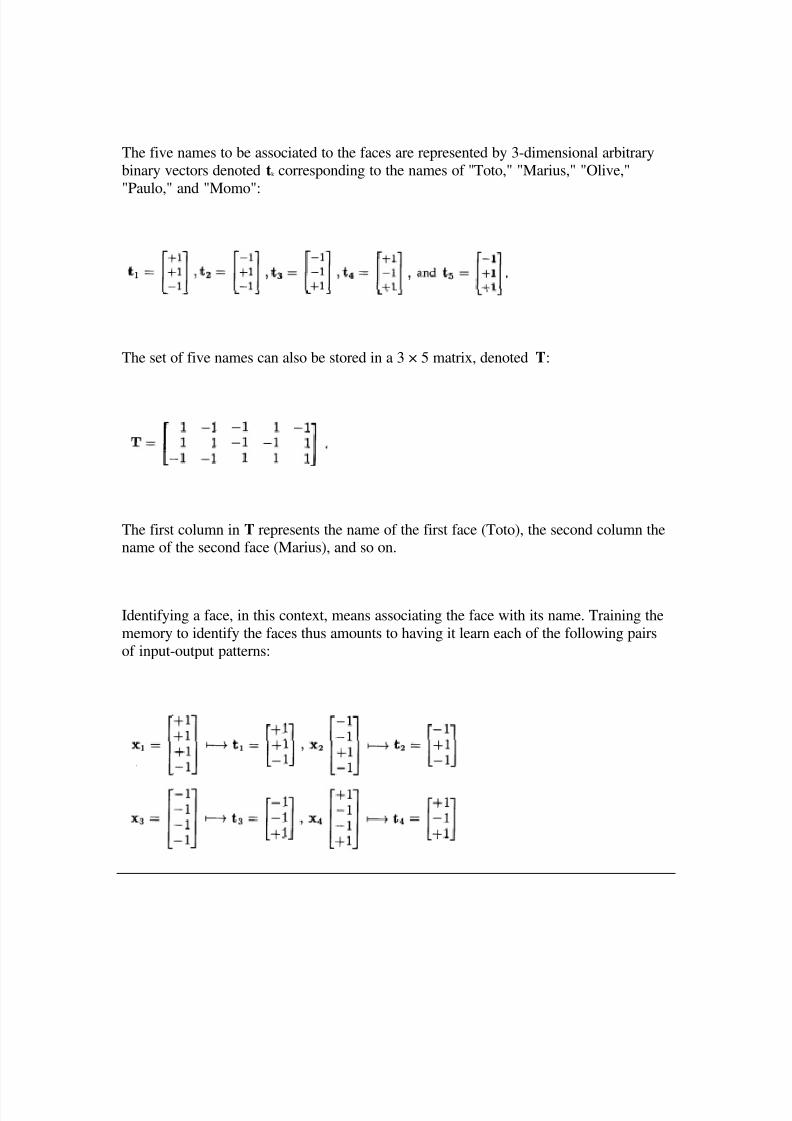
The five names to be associated to the faces are represented by 3-dimensional arbitrary

binary vectors denoted tk corresponding to the names of ''Toto," "Marius," "Olive,"

"Paulo," and "Momo":

The set of five names can also be stored in a 3 × 5 matrix, denoted T:

The first column in T represents the name of the first face (Toto), the second column thename of the second face (Marius), and so on.

Identifying a face, in this context, means associating the face with its name. Training the

memory to identify the faces thus amounts to having it learn each of the following pairs

of input-output patterns:



Page 51

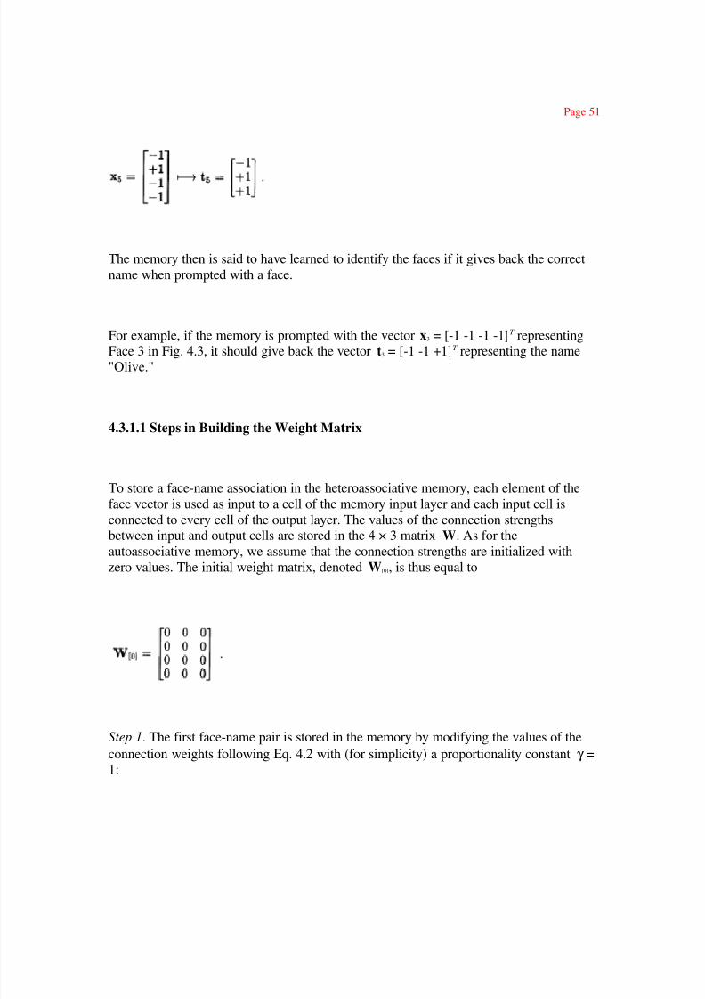
The memory then is said to have learned to identify the faces if it gives back the correct

name when prompted with a face.

For example, if the memory is prompted with the vector x3 = [-1 -1 -1 -1]T representing

Face 3 in Fig. 4.3, it should give back the vector t3 = [-1 -1 +1]T representing the name"Olive."

4.3.1.1 Steps in Building the Weight Matrix

To store a face-name association in the heteroassociative memory, each element of the

face vector is used as input to a cell of the memory input layer and each input cell is

connected to every cell of the output layer. The values of the connection strengthsbetween input and output cells are stored in the 4 × 3 matrix W. As for the

autoassociative memory, we assume that the connection strengths are initialized with

zero values. The initial weight matrix, denoted W[0], is thus equal to

Step 1. The first face-name pair is stored in the memory by modifying the values of the

connection weights following Eq. 4.2 with (for simplicity) a proportionality constant γ =1:



Observation of W[1] shows that each time an input and an output unit are both positive orboth negative, the weight between the two units increases by +1 and each time an input

and an output unit have opposite values, the weight between the two units decreases by

1.

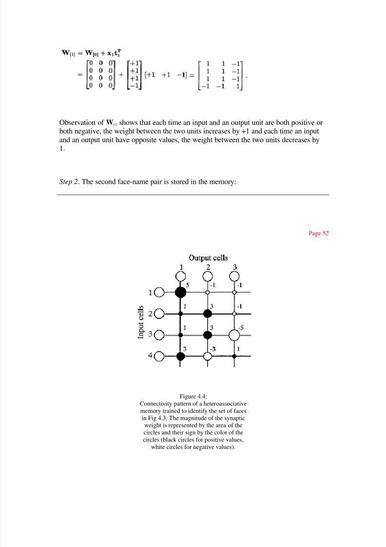
Step 2. The second face-name pair is stored in the memory:

Page 52

Figure 4.4:

Connectivity pattern of a heteroassociative

memory trained to identify the set of faces

in Fig 4.3. The magnitude of the synaptic

weight is represented by the area of the

circles and their sign by the color of the

circles (black circles for positive values,

white circles for negative values).



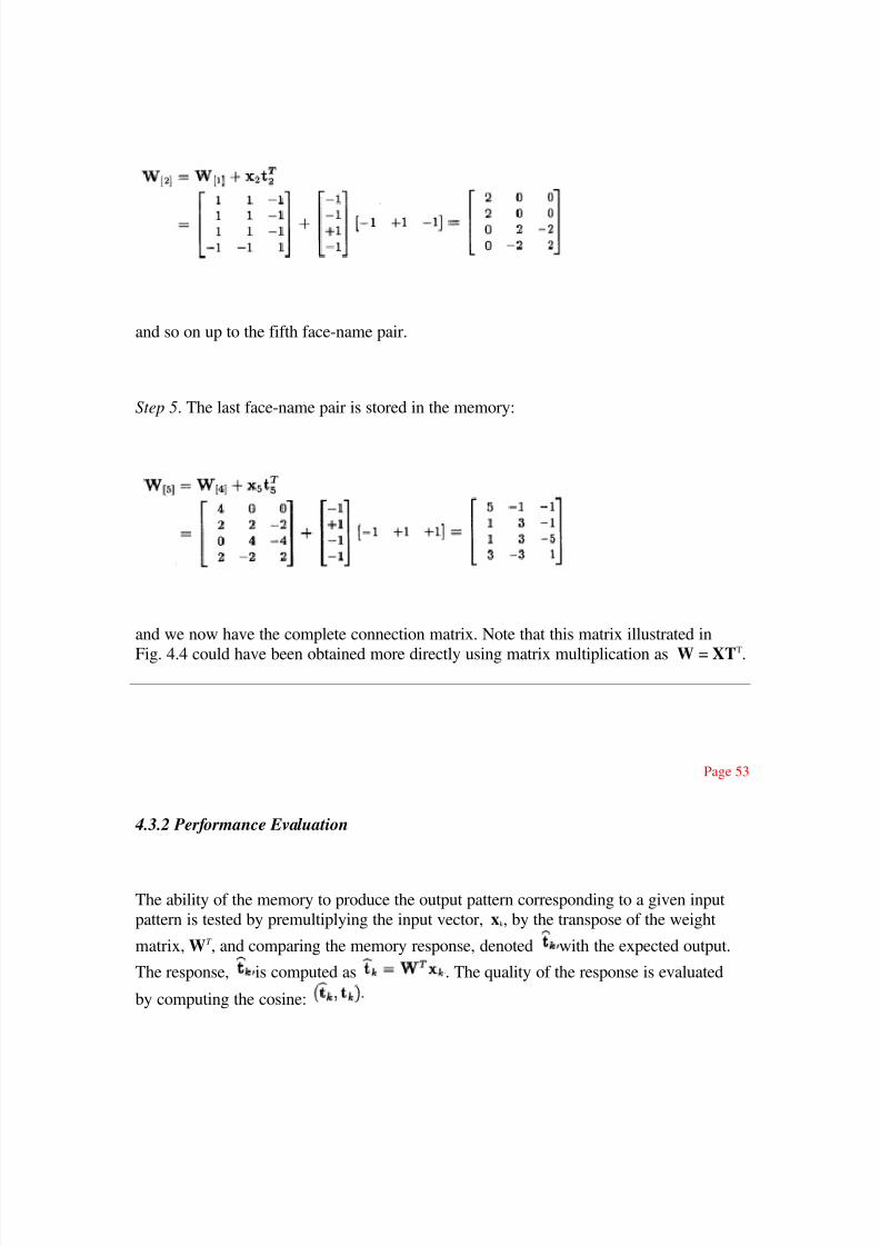
and so on up to the fifth face-name pair.

Step 5. The last face-name pair is stored in the memory:

and we now have the complete connection matrix. Note that this matrix illustrated in

Fig. 4.4 could have been obtained more directly using matrix multiplication as W = XTT

.

Page 53

4.3.2 Performance Evaluation

The ability of the memory to produce the output pattern corresponding to a given input

pattern is tested by premultiplying the input vector, xk , by the transpose of the weight

matrix, WT , and comparing the memory response, denoted with the expected output.

The response, is computed as . The quality of the response is evaluated

by computing the cosine:



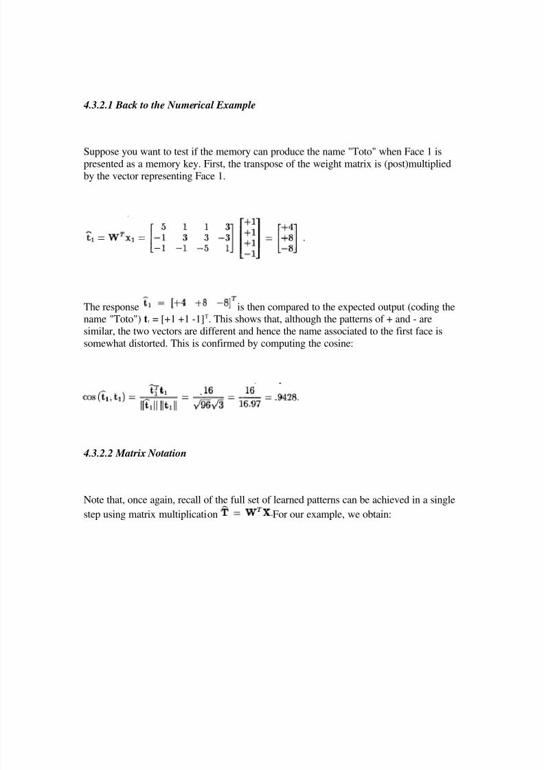
4.3.2.1 Back to the Numerical Example

Suppose you want to test if the memory can produce the name "Toto" when Face 1 is

presented as a memory key. First, the transpose of the weight matrix is (post)multiplied

by the vector representing Face 1.

The response is then compared to the expected output (coding thename "Toto") t1 = [+1 +1 -1]T. This shows that, although the patterns of + and - aresimilar, the two vectors are different and hence the name associated to the first face is

somewhat distorted. This is confirmed by computing the cosine:

4.3.2.2 Matrix Notation

Note that, once again, recall of the full set of learned patterns can be achieved in a single

step using matrix multiplication For our example, we obtain:



where the first column is the response of the memory to Face 1, the second column the

response of the memory to Face 2, and so on.

Page 54

4.3.3 Orthogonality and Crosstalk

Comparing the response matrix from the previous section to the vectors coding the face

names shows that none of the names associated with the faces is perfectly recalled. Thishappens because when the input vectors are not orthogonal (see Section 3.6.3 on page

33), the memory adds some noise to the expected patterns. Precisely:

The term is the interference or crosstalk between the response

corresponding to the input pattern and the responses corresponding to the other storedpatterns. When all the input patterns are pairwise orthogonal, all the scalar products

between pairs of different vectors are equal to zero and hence In this

case, the response of the memory to an input pattern is equal to the expected output

amplified by the scalar product of the input vector and itself . If the input pattern

is normalized such that , the response of the memory is the expected output.



If the input patterns are not orthogonal, the response of the memory is equal to the

expected output amplified by the scalar product of the input vector and itself plus

the crosstalk component: . The magnitude of the crosstalk depends on the

similarity or correlation between the input patterns: The larger the similarity between theinput patterns, the larger the crosstalk.

4.4 The Widrow-Hoff Learning Rule

The performance of the memory can be improved by using an error correction learning

rule instead of the simple Hebbian learning rule. In this section we show how to extend

the Widrow-Hoff learning rule, presented in Chapters 2 and 3, to the more general caseof heteroassociative memories. Remember that the Widrow-Hoff learning rule adjuststhe weights of the connections between cells so as to minimize the error sum of squares

between the responses of the memory and the expected responses. The values of the

weights are iteratively corrected using, as an error term, the difference between theexpected output and the answer of the memory. This algorithm can be used either in a

single stimulus learning mode (i.e., the error

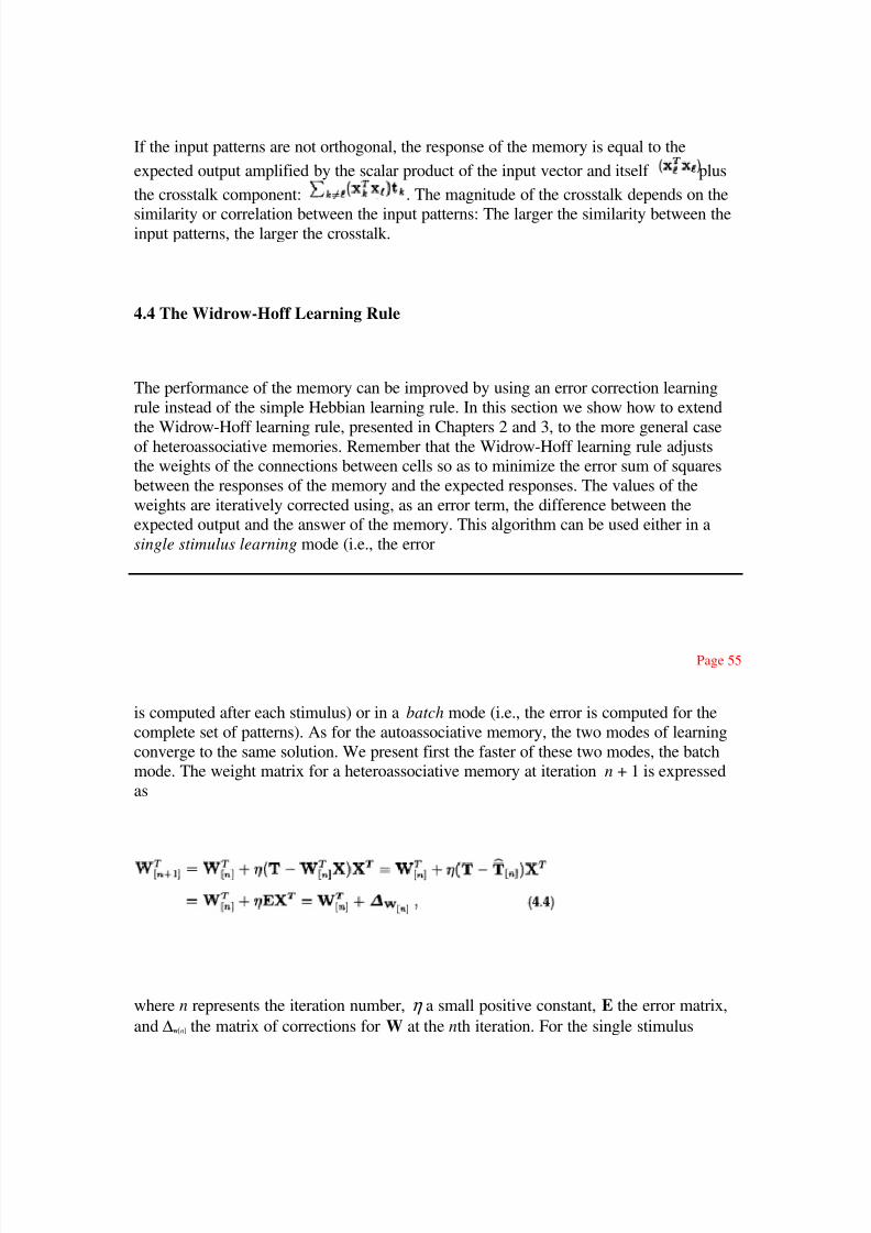
Page 55

is computed after each stimulus) or in a batch mode (i.e., the error is computed for the

complete set of patterns). As for the autoassociative memory, the two modes of learning

converge to the same solution. We present first the faster of these two modes, the batchmode. The weight matrix for a heteroassociative memory at iteration n + 1 is expressed

as

where n represents the iteration number, η a small positive constant, E the error matrix,

and ∆w[n] the matrix of corrections for W at the nth iteration. For the single stimulus



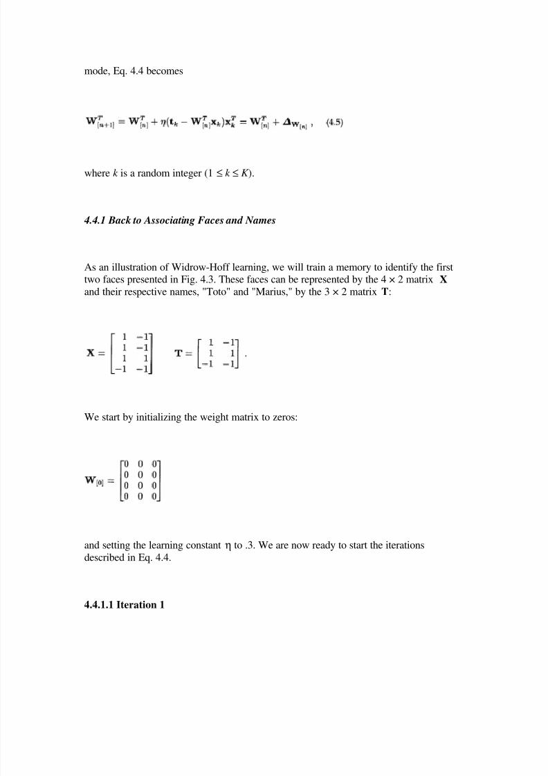
mode, Eq. 4.4 becomes

where k is a random integer (1 ≤ k ≤ K ).

4.4.1 Back to Associating Faces and Names

As an illustration of Widrow-Hoff learning, we will train a memory to identify the firsttwo faces presented in Fig. 4.3. These faces can be represented by the 4 × 2 matrix X

and their respective names, "Toto" and "Marius," by the 3 × 2 matrix T:

We start by initializing the weight matrix to zeros:

and setting the learning constant η to .3. We are now ready to start the iterationsdescribed in Eq. 4.4.

4.4.1.1 Iteration 1



Step 1: Identify the faces

Page 56

Step 2: Compute the error

Step 3: Compute the matrix of corrections

Step 4: Update the weight matrix



4.4.1.2 Iteration 16

Et voilà! The faces are perfectly identified after 16 iterations.

Page 57

4.4.2 Widrow-Hoff and Eigendecomposition

As for the autoassociative memory, the Widrow-Hoff learning rule can be expressed

from the singular value decomposition (SVD) of X. Precisely, the batch mode version (cf .Eq. 4.4 on page 55) can be implemented as



where n is the iteration number, U is the matrix of eigenvectors of XXT , V is the matrix

of eigenvectors of XT X, and ∆ is the diagonal matrix of singular values of X (for anotation refresher, see also Section 3.10 pages 41 ff .). For stimulus mode learning, Eq.

4.6 gives the state of the matrix after the nth learning epoch.

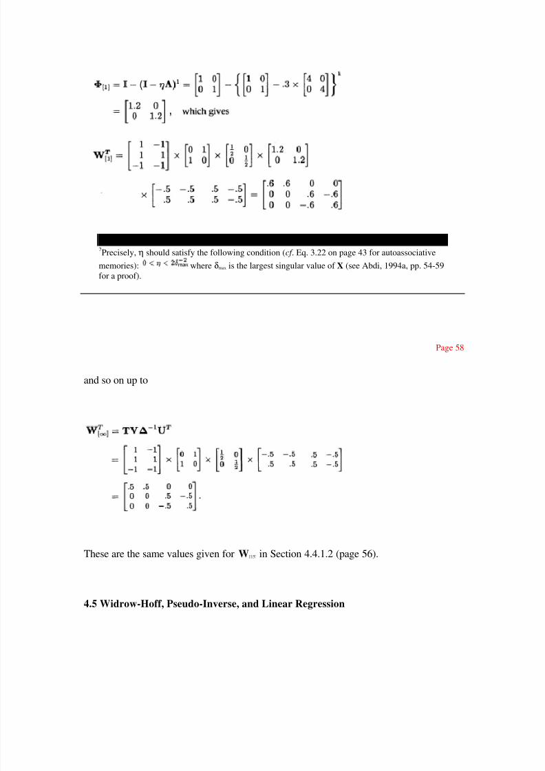
When η is properly chosen,2 φφφφ[n] converges to I and W becomes

For the previous example, the SVD of X gives

With a learning constant η = .3, the weight matrix at iteration 1 is obtained as

with



2Precisely, η should satisfy the following condition (cf . Eq. 3.22 on page 43 for autoassociative

memories): where δmax is the largest singular value of X (see Abdi, 1994a, pp. 54-59for a proof).

Page 58

and so on up to

These are the same values given for W[15] in Section 4.4.1.2 (page 56).

4.5 Widrow-Hoff, Pseudo-Inverse, and Linear Regression



4.5.1 Overview

Remember that the goal of a heteroassociator is to learn the mapping between pairs of input-output patterns so that the correct output is produced when a given pattern ispresented as a memory key. Formally, this goal is achieved by finding the connection

weights between the input and output units so that

In the previous sections we have seen that Hebbian learning is one way of finding thevalues of W. However, when the input patterns are not orthogonal, this learning

mechanism suffers from interference or crosstalk and produces some errors. As we

showed, this problem can be overcome by using the Widrow-Hoff error correctionlearning rule. In this section we show that an equivalent way of finding the values of W

is to solve Eq. 4.8. If the matrix X has an inverse,3 the solution is simply

However, in most applications, the matrix of stimuli X does not have an inverse. For

example, the 4 × 2 face matrix X presented in the previous example, is obviously not a

square matrix and hence is not invertible. In that case, we want to find the values of W such that the response produced by the memory will be as similar as possible to the

expected response. More formally, we want to find W such that

3Remember that only full rank square matrices have an inverse.

Page 58



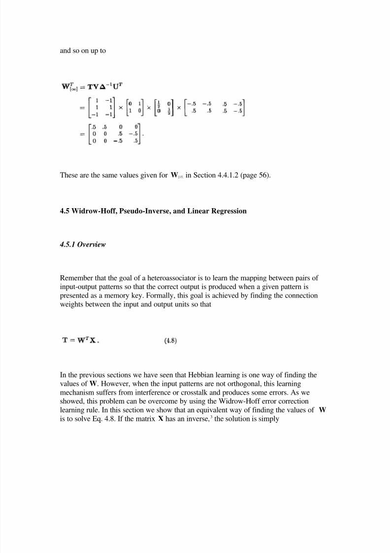
and so on up to

These are the same values given for W[15] in Section 4.4.1.2 (page 56).

4.5 Widrow-Hoff, Pseudo-Inverse, and Linear Regression

4.5.1 Overview

Remember that the goal of a heteroassociator is to learn the mapping between pairs of input-output patterns so that the correct output is produced when a given pattern is

presented as a memory key. Formally, this goal is achieved by finding the connection

weights between the input and output units so that

In the previous sections we have seen that Hebbian learning is one way of finding the

values of W

. However, when the input patterns are not orthogonal, this learningmechanism suffers from interference or crosstalk and produces some errors. As weshowed, this problem can be overcome by using the Widrow-Hoff error correction

learning rule. In this section we show that an equivalent way of finding the values of W

is to solve Eq. 4.8. If the matrix X has an inverse,3 the solution is simply



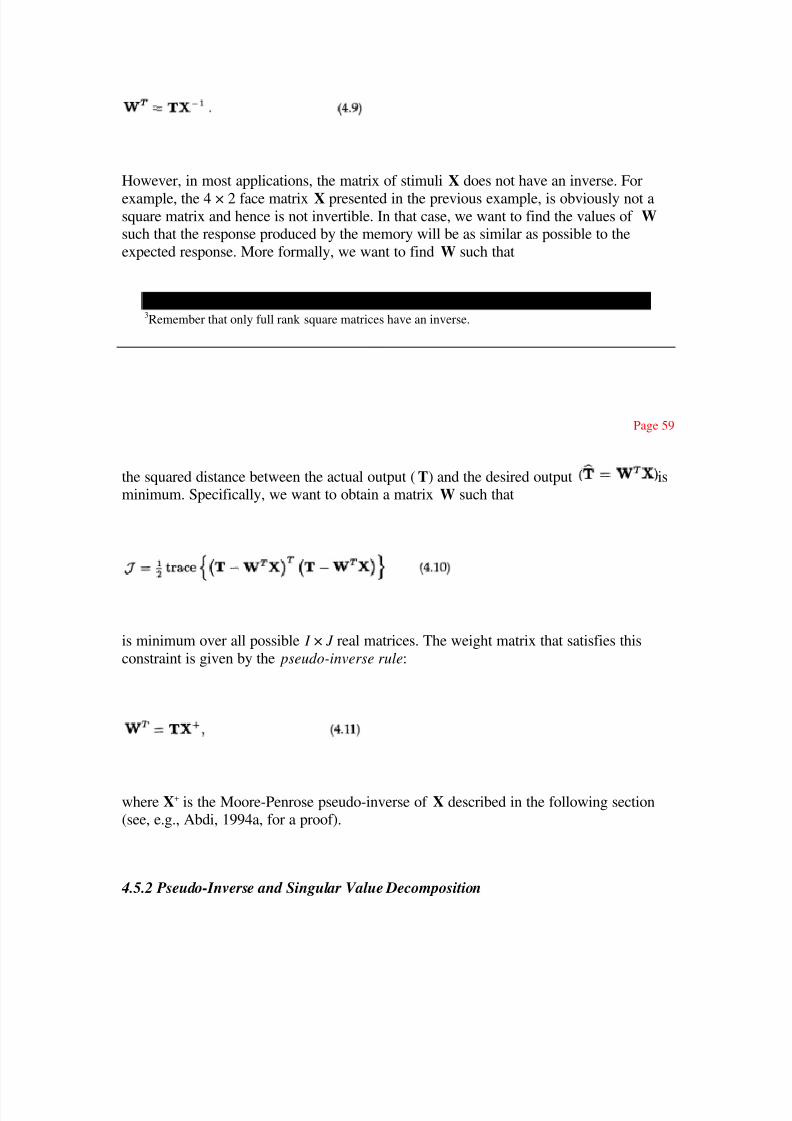
However, in most applications, the matrix of stimuli X does not have an inverse. For

example, the 4 × 2 face matrix X presented in the previous example, is obviously not asquare matrix and hence is not invertible. In that case, we want to find the values of W such that the response produced by the memory will be as similar as possible to the

expected response. More formally, we want to find W such that

3Remember that only full rank square matrices have an inverse.

Page 59

the squared distance between the actual output (T) and the desired output isminimum. Specifically, we want to obtain a matrix W such that

is minimum over all possible I × J real matrices. The weight matrix that satisfies this

constraint is given by the pseudo-inverse rule:

where X+ is the Moore-Penrose pseudo-inverse of X described in the following section(see, e.g., Abdi, 1994a, for a proof).

4.5.2 Pseudo-Inverse and Singular Value Decomposition



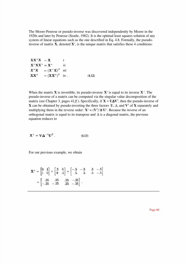
The Moore-Penrose or pseudo-inverse was discovered independently by Moore in the

1920s and later by Penrose (Searle, 1982). It is the optimal least squares solution of anysystem of linear equations such as the one described in Eq. 4.8. Formally, the pseudo-

inverse of matrix X, denoted X+, is the unique matrix that satisfies these 4 conditions:

When the matrix X is invertible, its pseudo-inverse X+

is equal to its inverse X-1

. Thepseudo-inverse of a matrix can be computed via the singular value decomposition of the

matrix (see Chapter 3, pages 41 ff .). Specifically, if X = U∆∆∆∆VT , then the pseudo-inverse of

X can be obtained by pseudo-inverting the three factors U, ∆, and VT of X separately and

multiplying them in the reverse order: X+ = (VT )+∆∆∆∆+U+. Because the inverse of an

orthogonal matrix is equal to its transpose and ∆ is a diagonal matrix, the previous

equation reduces to

For our previous example, we obtain

Page 60



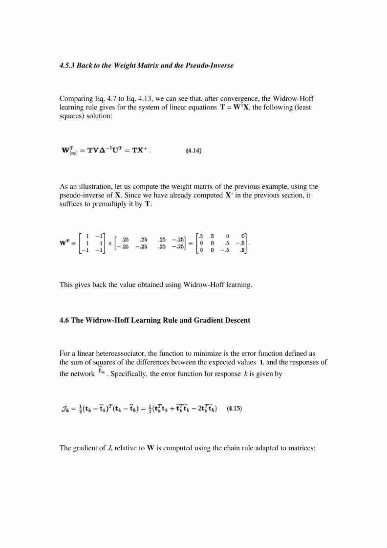
4.5.3 Back to the Weight Matrix and the Pseudo-Inverse

Comparing Eq. 4.7 to Eq. 4.13, we can see that, after convergence, the Widrow-Hoff learning rule gives for the system of linear equations T = WTX, the following (leastsquares) solution:

As an illustration, let us compute the weight matrix of the previous example, using the

pseudo-inverse of X. Since we have already computed X+ in the previous section, itsuffices to premultiply it by T:

This gives back the value obtained using Widrow-Hoff learning.

4.6 The Widrow-Hoff Learning Rule and Gradient Descent

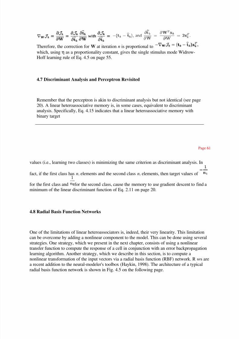
For a linear heteroassociator, the function to minimize is the error function defined as

the sum of squares of the differences between the expected values tk and the responses of

the network . Specifically, the error function for response k is given by

The gradient of J k relative to W is computed using the chain rule adapted to matrices:



Therefore, the correction for W at iteration n is proportional to

which, using η as a proportionality constant, gives the single stimulus mode Widrow-

Hoff learning rule of Eq. 4.5 on page 55.

4.7 Discriminant Analysis and Perceptron Revisited

Remember that the perceptron is akin to discriminant analysis but not identical (see page

20). A linear heteroassociative memory is, in some cases, equivalent to discriminantanalysis. Specifically, Eq. 4.15 indicates that a linear heteroassociative memory with

binary target

Page 61

values (i.e., learning two classes) is minimizing the same criterion as discriminant analysis. In

fact, if the first class has n1 elements and the second class n2 elements, then target values of

for the first class and for the second class, cause the memory to use gradient descent to find aminimum of the linear discriminant function of Eq. 2.11 on page 20.

4.8 Radial Basis Function Networks

One of the limitations of linear heteroassociators is, indeed, their very linearity. This limitation

can be overcome by adding a nonlinear component to the model. This can be done using severalstrategies. One strategy, which we present in the next chapter, consists of using a nonlineartransfer function to compute the response of a cell in conjunction with an error backpropagation

learning algorithm. Another strategy, which we describe in this section, is to compute a

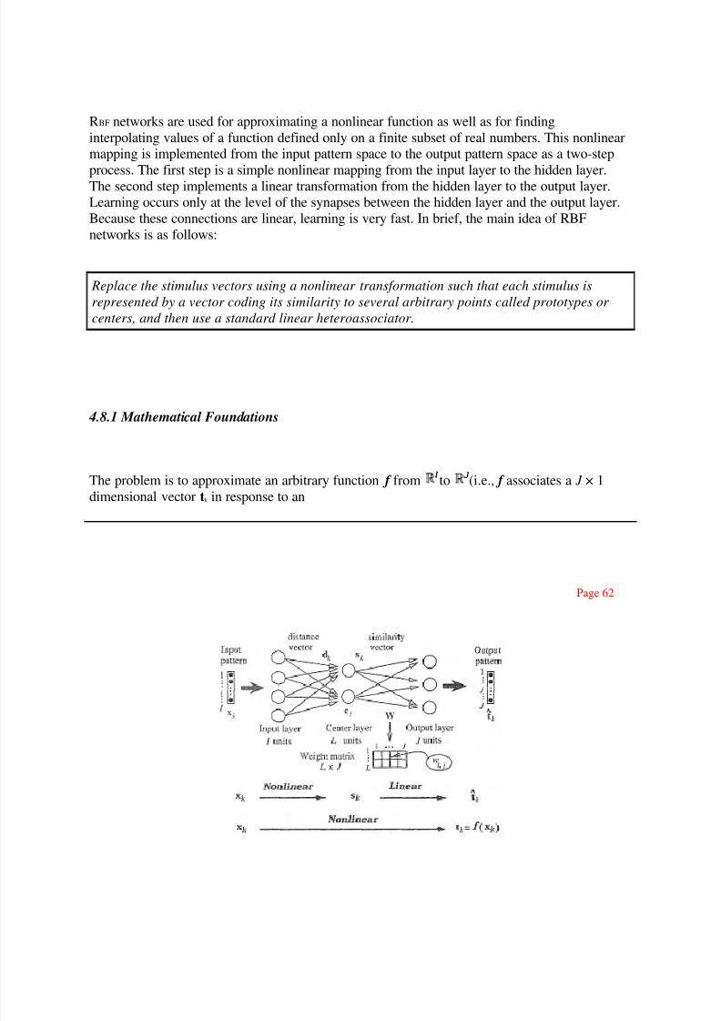
nonlinear transformation of the input vectors via a radial basis function (RBF) network. RBFs area recent addition to the neural-modeler's toolbox (Haykin, 1998). The architecture of a typical

radial basis function network is shown in Fig. 4.5 on the following page.



RBF networks are used for approximating a nonlinear function as well as for finding

interpolating values of a function defined only on a finite subset of real numbers. This nonlinearmapping is implemented from the input pattern space to the output pattern space as a two-step

process. The first step is a simple nonlinear mapping from the input layer to the hidden layer.

The second step implements a linear transformation from the hidden layer to the output layer.Learning occurs only at the level of the synapses between the hidden layer and the output layer.

Because these connections are linear, learning is very fast. In brief, the main idea of RBF

networks is as follows:

Replace the stimulus vectors using a nonlinear transformation such that each stimulus is

represented by a vector coding its similarity to several arbitrary points called prototypes or

centers, and then use a standard linear heteroassociator.

4.8.1 Mathematical Foundations

The problem is to approximate an arbitrary function f from to (i.e., f associates a J × 1

dimensional vector tk in response to an

Page 62



Figure 4.5:

The architecture of a typical radial basis function network.

The hidden layer computes the distance from the input to each

of the centers (each center corresponds to a cell of the hiddenlayer). The cells of the hidden layer transform their activation

(i.e., the distance from the input) into a response using

a nonlinear transformation (typically a Gaussian function).

The cells of the output layer behave like a standard

linear heteroassociator.

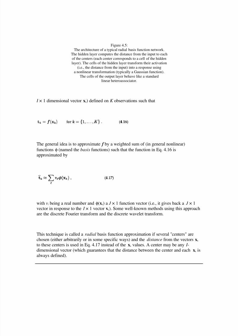
I × 1 dimensional vector xk ) defined on K observations such that

The general idea is to approximate f by a weighted sum of (in general nonlinear)

functions φ (named the basis functions) such that the function in Eq. 4.16 isapproximated by

with vl being a real number and φ(xk ) a J × 1 function vector (i.e., it gives back a J × 1vector in response to the I × 1 vector xk ). Some well-known methods using this approach

are the discrete Fourier transform and the discrete wavelet transform.

This technique is called a radial basis function approximation if several ''centers" arechosen (either arbitrarily or in some specific ways) and the distance from the vectors xk to these centers is used in Eq. 4.17 instead of the xk values. A center may be any I -

dimensional vector (which guarantees that the distance between the center and each xk is

always defined).



Page 63

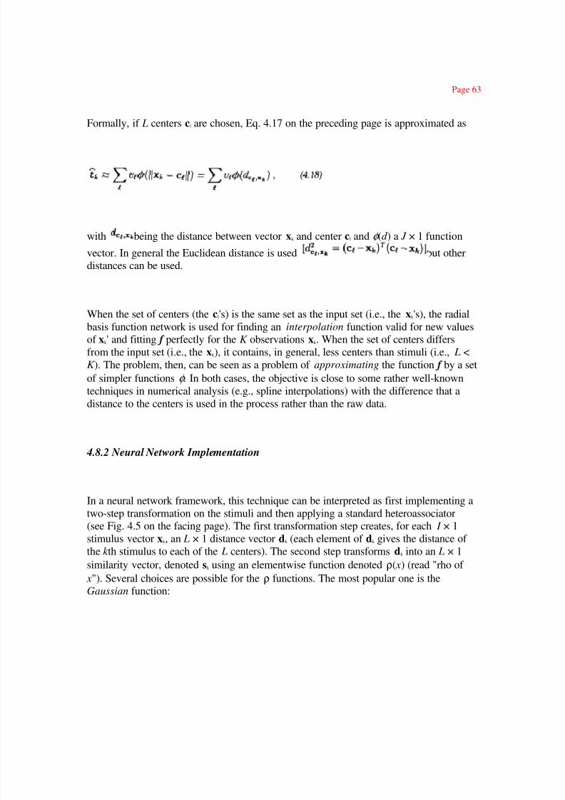
Formally, if L centers cl are chosen, Eq. 4.17 on the preceding page is approximated as

with being the distance between vector xk and center cl and φ (d ) a J × 1 function

vector. In general the Euclidean distance is used but otherdistances can be used.

When the set of centers (the cl's) is the same set as the input set (i.e., the xk 's), the radial

basis function network is used for finding an interpolation function valid for new valuesof xk ' and fitting f perfectly for the K observations xk . When the set of centers differs

from the input set (i.e., the xk ), it contains, in general, less centers than stimuli (i.e., L <

K ). The problem, then, can be seen as a problem of approximating the function f by a set

of simpler functions φ . In both cases, the objective is close to some rather well-known

techniques in numerical analysis (e.g., spline interpolations) with the difference that a

distance to the centers is used in the process rather than the raw data.

4.8.2 Neural Network Implementation

In a neural network framework, this technique can be interpreted as first implementing a

two-step transformation on the stimuli and then applying a standard heteroassociator(see Fig. 4.5 on the facing page). The first transformation step creates, for each I × 1

stimulus vector xk , an L × 1 distance vector dk (each element of dk gives the distance of

the k th stimulus to each of the L centers). The second step transforms dk into an L × 1

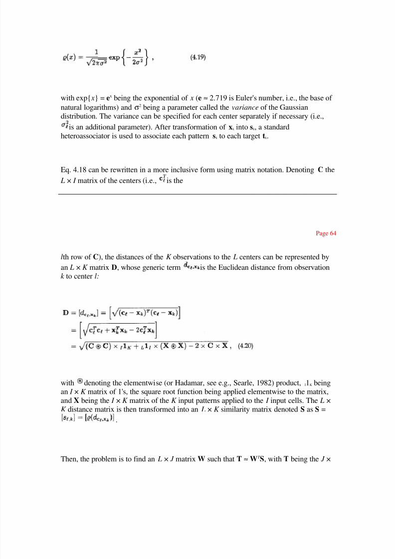
similarity vector, denoted sk using an elementwise function denoted ρ( x) (read "rho of

x"). Several choices are possible for the ρ functions. The most popular one is the

Gaussian function:



with exp{ x} = ex being the exponential of x (e ≈ 2.719 is Euler's number, i.e., the base of natural logarithms) and σ2 being a parameter called the variance of the Gaussiandistribution. The variance can be specified for each center separately if necessary (i.e.,

is an additional parameter). After transformation of xk into sk , a standard

heteroassociator is used to associate each pattern sk to each target tk .

Eq. 4.18 can be rewritten in a more inclusive form using matrix notation. Denoting C the

L × I matrix of the centers (i.e., is the

Page 64

lth row of C), the distances of the K observations to the L centers can be represented by

an L × K matrix D, whose generic term is the Euclidean distance from observationk to center l:

with denoting the elementwise (or Hadamar, see e.g., Searle, 1982) product, I1K being

an I × K matrix of 1's, the square root function being applied elementwise to the matrix,and X being the I × K matrix of the K input patterns applied to the I input cells. The L ×

K distance matrix is then transformed into an L × K similarity matrix denoted S as S =

.

Then, the problem is to find an L × J matrix W such that T ≈ WT S, with T being the J ×



K matrix of the K output patterns. If S is a nonsingular square matrix, the solution is

given by (from Eq. 4.9 on page 58) WT = TS-1. If S is singular or rectangular, a least

squares approximation is given by (from Eq. 4.11 on page 59)

with S+ being the pseudo-inverse of S. One reason for the popularity of the Gaussian

transformation is that it ensures that when D is a square matrix, and when the centers arenot redundant (i.e., no center is present twice), then the matrix S is not only nonsingular

but also positive definite (Michelli, 1986). Note that, even though D is a distance matrix,

it is in general not full rank and not even positive semi-definite, which is the main

motivation for transforming the distance to the centers into a similarity.

If the testing set is different from the learning set, then the distance from each element of the testing set to each of the centers needs to be computed. This distance is then

transformed into a similarity using the ρ function before being multiplied by the matrix

W to give the estimation of the response to the testing set by the radial basis functionnetwork. The response of the network to a pattern x (old or new) is obtained by first

transforming this pattern into d (the vector of distance from x to the L centers cl), then

transforming d into a similarity vector s, and finally obtaining the response as

Page 65

If we denote by wl the J × 1 vector storing the lth column of WT , Eq. 4.18 on page 63 canbe rewritten as



This shows that this variation of the linear heteroassociator implements the technique of

radial basis function interpolation.

4.8.3 Radial Basis Function Networks: an Example

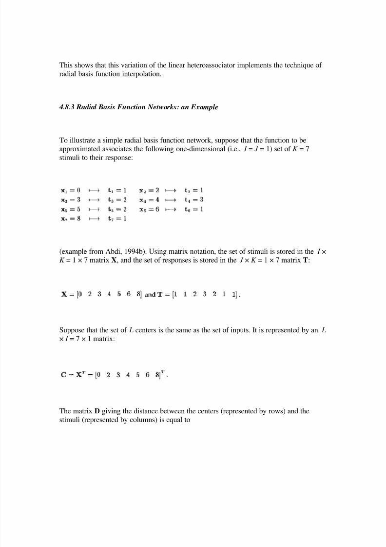
To illustrate a simple radial basis function network, suppose that the function to beapproximated associates the following one-dimensional (i.e., I = J = 1) set of K = 7

stimuli to their response:

(example from Abdi, 1994b). Using matrix notation, the set of stimuli is stored in the I ×

K = 1 × 7 matrix X, and the set of responses is stored in the J × K = 1 × 7 matrix T:

Suppose that the set of L centers is the same as the set of inputs. It is represented by an L

× I = 7 × 1 matrix:

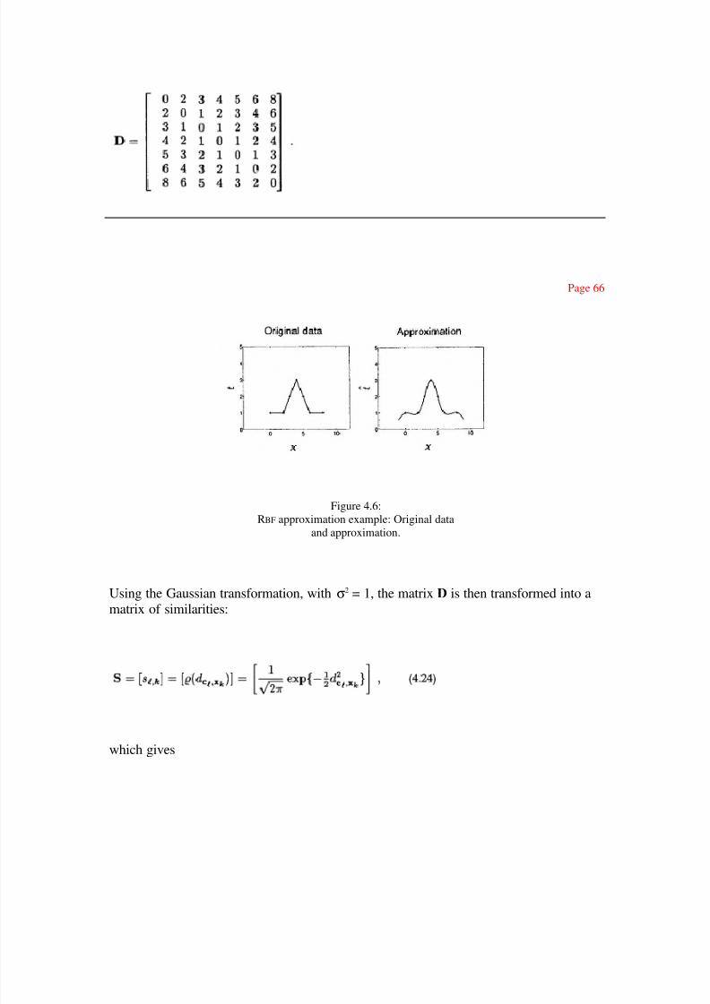
The matrix D giving the distance between the centers (represented by rows) and the

stimuli (represented by columns) is equal to



Page 66

Figure 4.6:

RBF approximation example: Original data

and approximation.

Using the Gaussian transformation, with σ2 = 1, the matrix D is then transformed into amatrix of similarities:

which gives



The optimum matrix of weights, which would be found by a heteroassociator using

Widrow-Hoff learning, can be computed by first inverting the matrix S:

and then premultiplying S-1 by T:

These weights can be used to compute the network response to a training stimulus (in

this example, the training stimulus will give

Page 67

a response which matches the target perfectly), or they can be used to approximate a

response to a stimulus not in the training set. To calculate the answer of the radial basisfunction network to a stimulus (old or new), it suffices to compute the distance vector

from that stimulus to the seven centers, to transform it into a similarity vector using the

Gaussian function, and to premultiply it by the matrix WT . For example, the response of

the network to the new stimulus x = 1 (where each element of d is the distance from x to



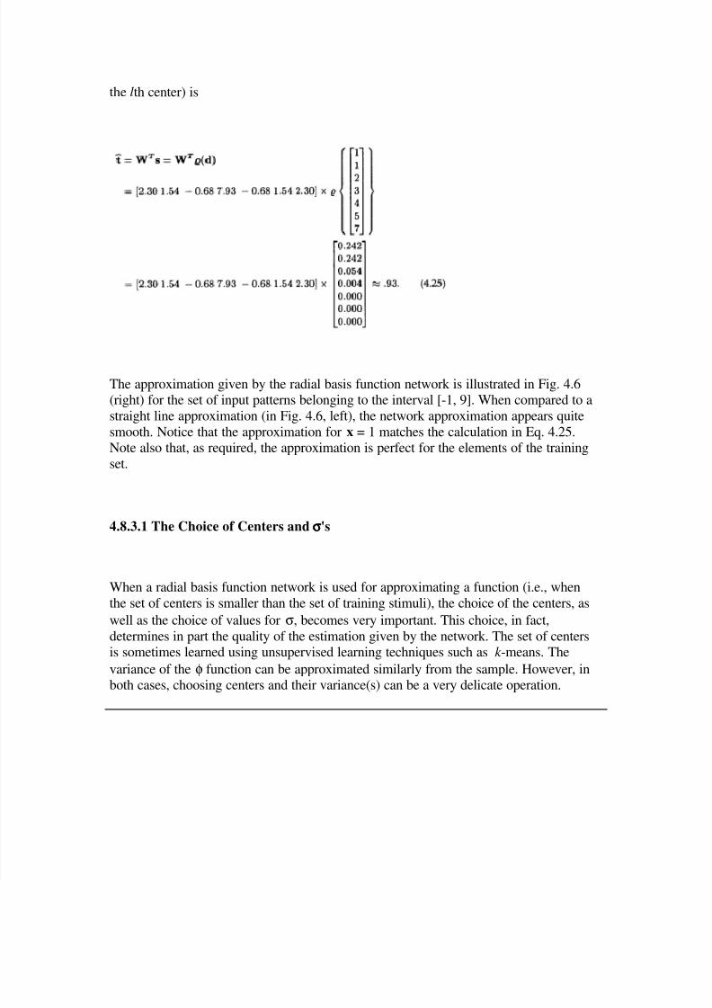
the lth center) is

The approximation given by the radial basis function network is illustrated in Fig. 4.6(right) for the set of input patterns belonging to the interval [-1, 9]. When compared to a

straight line approximation (in Fig. 4.6, left), the network approximation appears quite

smooth. Notice that the approximation for x = 1 matches the calculation in Eq. 4.25.Note also that, as required, the approximation is perfect for the elements of the training

set.

4.8.3.1 The Choice of Centers and σσσσ's

When a radial basis function network is used for approximating a function (i.e., when

the set of centers is smaller than the set of training stimuli), the choice of the centers, as

well as the choice of values for σ, becomes very important. This choice, in fact,

determines in part the quality of the estimation given by the network. The set of centersis sometimes learned using unsupervised learning techniques such as k -means. The

variance of the φ function can be approximated similarly from the sample. However, inboth cases, choosing centers and their variance(s) can be a very delicate operation.

Documents

Learning and RBF