Learn About One-Way MANOVA in SPSS With Data From the

Learn About One-Way MANOVA in

SPSS With Data From the

Canadian Fuel Consumption

Report (2015)

© 2015 SAGE Publications, Ltd. All Rights Reserved.

This PDF has been generated from SAGE Research Methods Datasets.

Learn About One-Way MANOVA in

SPSS With Data From the

Canadian Fuel Consumption

Report (2015)

Student Guide

Introduction

This example describes one-way MANOVA, discusses the assumptions

underlying it, and shows how to estimate and interpret one-way MANOVA models.

We illustrate one-way MANOVA using a subset of data from the 2015 Fuel

Consumption Ratings from Natural Resources Canada (http://open.canada.ca/

data/en/dataset/98f1a129-f628-4ce4-b24d-6f16bf24dd64).

Specifically, we test whether the CO2 emissions and highway fuel consumption

of an automobile both differ based on the number of engine cylinders in that

automobile. Understanding how features of automobile engines impact their

average emissions and fuel consumption is important for making policy decisions

about fuel economy standards and carbon emissions.

What Is One-Way MANOVA?

One-way MANOVA is a statistical procedure for comparing the means of two

or more continuous variables across two or more subsets of the data. Those

subsets are generally defined by categories from a categorical variable in the

dataset. One-way MANOVA is an extension of one-way ANOVA, which analyses

the difference in means for a single continuous variable across subsets of the

SAGE

2015 SAGE Publications, Ltd. All Rights Reserved.

SAGE Research Methods Datasets Part

1

Page 2 of 13 Learn About One-Way MANOVA in SPSS With Data From the Canadian

Fuel Consumption Report (2015)

http://open.canada.ca/data/en/dataset/98f1a129-f628-4ce4-b24d-6f16bf24dd64

http://open.canada.ca/data/en/dataset/98f1a129-f628-4ce4-b24d-6f16bf24dd64

data. In examining two or more continuous variables simultaneously, one-way

MANOVA allows the researcher to account for any possible correlation between

those two variables while computing and comparing their means.

For example, you might be interested in whether three different treatment options

led to differences in people’s body mass index (BMI) and cholesterol levels.

BMI and cholesterol levels are likely to be correlated, which one-way MANOVA

accommodates. In this example, one-way MANOVA allows you to examine the

general question of whether the impact of these three treatments on patient health

overall (as measured by BMI and cholesterol levels) differed in a statistically

significant way. This is a multivariate hypothesis test and is most commonly

evaluated using Wilks’ Lambda and its associated p-value. It requires additional

steps to focus in on which particular treatments differed from each other and

whether they differed on BMI, cholesterol levels, or both.

When computing formal statistical tests, it is customary to define the null

hypothesis (H0) to be tested. In this case, the standard null hypothesis is that the

means of the continuous variables in question do not differ across the different

groups defined by the categorical variable in question. Some difference is

expected to appear in any one sample of data due to random chance in sampling.

Thus, the question becomes whether the observed difference is large enough to

be considered statistically significant.

“Large enough” is typically defined as selecting a critical value for the test statistic

such that there is less than a 0.05 probability that the result observed in the

sample of data occurred strictly due to random chance. When this probability, or

p-value, is estimated to be less than 0.05, this would generally lead researchers to

reject the null hypothesis (H0) of no difference and conclude that there likely is a

relationship between the categorical variable in question and the set of continuous

variables being analyzed.

SAGE



1



Estimating One-Way MANOVA

The estimation of one-way MANOVA is a complicated extension of one-way

ANOVA. Rather than work through the math, we focus on the intuition behind the

method. One-way MANOVA focuses on the variability in two or more continuous

variables between groups as determined by a categorical variable of interest

compared to variation in those variables within those groups. That variability is

expressed in terms of sums of squares. Specifically, values of each continuous

variable are expressed as differences from their respective means, with each

difference then being squared, and all of those squared values being summed up.

These sums of squares account for the variance in each continuous variable, but

because we have more than one continuous variable of interest, MANOVA also

includes the covariance between the continuous variables.

MANOVA compares the variance in the two continuous variables within groups

to the variance between groups to evaluate whether the groups differ from each

other in a statistically significant way. If there is little variance within groups,

but substantial variance between them, then the distribution of values for the

continuous variables for each group will not overlap with each other very much

and group means will differ significantly from each other. In contrast, if the ratio

of variance within the groups relative to the variance between the groups is high,

the distribution of values for the continuous variables for each group will overlap

considerably and the group means will not differ from each other.

Many statistical tests can be calculated to evaluate the null hypothesis in a

MANOVA model. They can generally be thought of as multivariate equivalents to

the model F-test routinely computed for one-way ANOVA.

This test evaluates the MANOVA overall. It cannot tell you which particular groups

differ from each other, and it cannot tell you whether the groups differ from each

other on one, some, or all of the continuous variables being analyzed. Thus

SAGE



1



most researchers who find a statistically significant result overall would conduct

some additional tests to look more closely at pairwise comparisons among groups

across all of the dependent variables.

Assumptions Behind the Method

Nearly every statistical test relies on some underlying assumptions, and they are

all affected by the mix of data you happen to have. Different textbooks present

the assumptions of one-way MANOVA in different ways, but we present them as

follows:

• The observations are independent of each other.

• The residuals of the continuous dependent variables are (approximately)

normally distributed within groups.

• Relationships between the continuous variables, if they exist, are linear.

• Variances and covariances of the continuous dependent variables are

equal across groups.

• Values of the continuous dependent variables within each group are

independent and identically distributed.

These are important assumptions to consider, though note that MANOVA is fairly

robust to moderate violations of the normality assumption.

Illustrative Example: Highway Fuel Consumption, CO2 Emissions,

and Engine Cylinders

This example explores whether the CO2 emissions and highway fuel consumption

of an automobile differ based on the number of engine cylinders in that

automobile. Understanding how features of automobile engines impact their

average emissions and fuel consumption is important for making policy decisions

about fuel economy standards and carbon emissions.

SAGE



1



This example therefore addresses the following research question:

Does the average highway fuel consumption and/or CO2 emissions of

an automobile differ depending on the number of engine cylinders in that

automobile?

This can be stated as a null hypothesis as well:

H0 = Whether an automobile has 4, 6, or 8 cylinders has no impact on its

average highway fuel consumption and average CO2 emissions.

The Data

This example uses three variables from the 2015 Fuel Consumption Report from

Natural Resources Canada:

• The highway fuel consumption of an automobile (fuelusehwy), measured in

liters per 100 kilometers.

• The CO2 emissions of an automobile (co2emissions), measured in grams

per kilometer.

• The number of cylinders in the automobile engine (cylinders468), either 4,

6, or 8.

The dataset includes 1082 observations. The highway fuel consumption is

measured in liters per 100 kilometers. In this dataset, it has a mean of

approximately 8.88 with a standard deviation of about 2.23. The CO2 emissions

of the automobile, measured in grams per kilometer, has a mean of approximately

244 with a standard deviation of about 55.7. Whether an automobile has 4,

6, or 8 cylinders is measured as a categorical variable, with 489 (45.19%) of

the automobiles having 4 cylinders, 384 (35.49%) of the automobiles having 6

cylinders, and 209 (19.32%) of the automobiles having 8 cylinders.

SAGE



1



Analyzing the Data

Before producing the MANOVA analysis, it is a good idea to look at each variable

separately. Figures 1 and 2 present histograms of CO2 emissions and highway

fuel consumption, respectively.

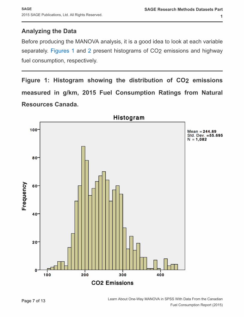
Figure 1: Histogram showing the distribution of CO2 emissions

measured in g/km, 2015 Fuel Consumption Ratings from Natural

Resources Canada.

SAGE



1



Figure 2: Histogram showing the distribution of highway fuel

consumption measured in l/100km, 2015 Fuel Consumption Ratings

from Natural Resources Canada.

Figure 1 shows that the majority of values for CO2 emissions fall below 275 grams

per kilometer, with the bulk of observations clustered around the mean of about

244 grams per kilometer. There are a few extreme values, with the largest being

437 grams per kilometer. Researchers may want to explore whether cases with

these extreme values have undue influence on the regression.

SAGE



1



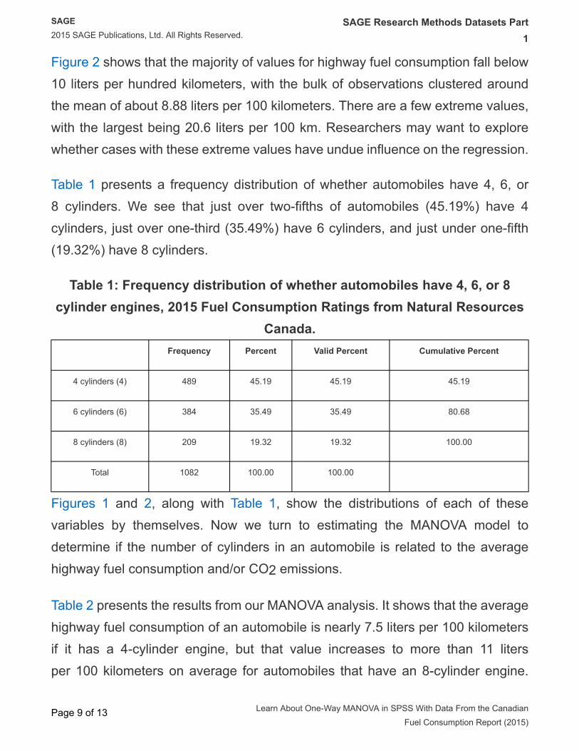
Figure 2 shows that the majority of values for highway fuel consumption fall below

10 liters per hundred kilometers, with the bulk of observations clustered around

the mean of about 8.88 liters per 100 kilometers. There are a few extreme values,

with the largest being 20.6 liters per 100 km. Researchers may want to explore

whether cases with these extreme values have undue influence on the regression.

Table 1 presents a frequency distribution of whether automobiles have 4, 6, or

8 cylinders. We see that just over two-fifths of automobiles (45.19%) have 4

cylinders, just over one-third (35.49%) have 6 cylinders, and just under one-fifth

(19.32%) have 8 cylinders.

Table 1: Frequency distribution of whether automobiles have 4, 6, or 8

cylinder engines, 2015 Fuel Consumption Ratings from Natural Resources

Canada.

Frequency Percent Valid Percent Cumulative Percent

4 cylinders (4) 489 45.19 45.19 45.19

6 cylinders (6) 384 35.49 35.49 80.68

8 cylinders (8) 209 19.32 19.32 100.00

Total 1082 100.00 100.00

Figures 1 and 2, along with Table 1, show the distributions of each of these

variables by themselves. Now we turn to estimating the MANOVA model to

determine if the number of cylinders in an automobile is related to the average

highway fuel consumption and/or CO2 emissions.

Table 2 presents the results from our MANOVA analysis. It shows that the average

highway fuel consumption of an automobile is nearly 7.5 liters per 100 kilometers

if it has a 4-cylinder engine, but that value increases to more than 11 liters

per 100 kilometers on average for automobiles that have an 8-cylinder engine.

SAGE



1



Similarly, Table 2 shows that the average automobile with 4 engine cylinders

emits about 200 grams of CO2 per kilometer, but the average automobile that

has 8 engine cylinders emits more, with average CO2 emissions of about 322

grams per kilometer. Finally, Table 2 reports a value of Wilks’ lambda of 0.324

and an associated p-value < 0.001. This low p-value would lead us to reject the

null hypothesis and conclude that whether an automobile has 4, 6, or 8 engine

cylinders is statistically significantly associated with the average highway fuel

consumption and/or amount of CO2 emissions.

Table 2: MANOVA results testing whether automobiles with 4, 6, and 8

engine cylinders differ in terms of average CO2 emissions (in grams per

kilometer) and/or highway fuel consumption (in liters per 100 kilometers),

2015 Fuel Consumption Report from Natural Resources Canada.

Mean Standard Deviation N

Highway fuel cons. (l/100km) 4 cylinders (4) 7.357 1.13 489

6 cylinders (6) 9.34 1.55 384

8 cylinders (8) 11.59 2.28 209

CO2 emissions (g/km) 4 cylinders 200.92 28.61 489

6 cylinders 258.18 27.79 384

8 cylinders 322.31 43.42 209

Wilk’s lambda 0.324 (p-value < 0.001)

Having rejected the overall null hypothesis, we turn to tests for each dependent

variable. In this example, we find an F-statistic of 1124 (p-value < 0.001) testing

the difference in average CO2 emissions for automobiles with 4, 6, and 8-cylinder

engines. Similarly, we find an F-statistic of 567 (p-value < 0.001) testing the

difference in average highway fuel consumption for automobiles with 4, 6, and

SAGE



1



8-cylinder engines. With such low p-values, both tests indicate statistically

significant differences in group means for both CO2 emissions and highway fuel

consumption.

In this example, we have three groups of vehicles based on the number of

cylinders each has. As a result, we can compute pairwise differences in means for

all possible two-way combinations of groups of vehicles for both CO2 emissions

and highway fuel consumption. We can also test them for statistical significance.

This most often involves employing Bonferroni’s adjustment to the hypothesis test.

The results are presented in Table 3. The results in Table 3 show that the means

for both CO2 emissions and highway fuel use are statistically significantly different

from each other for all possible pairwise comparisons based on whether a car’s

engine has 4, 6, or 8 cylinders.

Table 3: Pairwise comparisons between groups of vehicles based on

number of engine cylinders regarding average CO2 emissions (in grams

per kilometer) and highway fuel consumption (in liters per 100 kilometers),

2015 Fuel Consumption Report from Natural Resources Canada.

Variable Comparison Mean Diff. p-value

CO2 Emissions 4 to 6 Cylinders −57.26 0.000

4 to 8 Cylinders −121.39 0.000

6 to 8 Cylinders −64.12 0.000

Hwy Fuel Use 4 to 6 Cylinders −1.99 0.000

4 to 8 Cylinders −4.24 0.000

6 to 8 Cylinders −2.25 0.000

Presenting Results

SAGE



1



The results of a MANOVA can be presented as follows:

“We used a subset of data from the 2015 Fuel Consumption Report from Natural

Resources Canada to test the following null hypotheses:

H0 = Whether an automobile has 4, 6, or 8 engine cylinders has no

impact on its average highway fuel consumption and average CO2

emissions.

The dataset includes 1082 individual automobiles. Results presented in Table 2

show that the average highway fuel consumption of an automobile is nearly 7.5

liters per 100 kilometers if it has a 4-cylinder engine, but more than 11 liters

per 100 kilometers on average for automobiles that have an 8-cylinder engine.

Similarly, the average automobile with 4 engine cylinders emits about 200 grams

of CO2 per kilometer, while the average automobile that has 8 engine cylinders

emit more, with average CO2 emissions of about 322 grams per kilometer. Wilks’

lambda and its associated p-value lead us to reject the null hypothesis of no

differences among automobiles with 4, 6, and 8 engine cylinders for these two

variables. Subsequent testing demonstrates that both the difference in highway

fuel consumption and the difference in CO2 emissions are statistically significant.

Table 3 reports that every difference in CO2 emissions and highway fuel

consumption between all possible two-way comparisons between groups of

vehicles is statistically significant as well.”

Review

One-way MANOVA is a statistical procedure for comparing the means of two or

more continuous variables across two or more subsets of the data. Those subsets

are generally defined by categories from a categorical variable in the dataset.

One-way MANOVA begins with an overall test of the model, but then frequently

proceeds to tests associated with each continuous variable and across all pairwise

SAGE



1



comparisons of the subsets in question. One-way MANOVA is particularly useful

in situations where the two or more continuous dependent variables in question

are likely to be correlated with each other.

You should know:

• What types of variable are suitable for one-way MANOVA.

• The basic assumptions underlying one-way MANOVA.

• How to estimate and interpret a one-way MANOVA.

• How to report the results of a one-way MANOVA.

Your Turn

You can download this sample dataset along with a guide showing how to

estimate a multiple regression model using statistical software. The sample

dataset includes a variable called fuelusecity which measures fuel consumption

for city driving in liters per 100 kilometers, and another variable called fuel that

is a categorical variable measuring the type of fuel used by the vehicle. Try

producing your own one-way MANOVA by replacing fuelusehwy with fuelusecity

and cylinders468 with fuel.

SAGE



1



Documents

Learn About One-Way MANOVA in SPSS With Data From the